Testing Consumer Rationality using
Perfect Graphs and Oriented Discs

Abstract

Given a consumer data-set, the axioms of revealed preference proffer a binary test for rational behaviour. A natural (non-binary) measure of the degree of rationality exhibited by the consumer is the minimum number of data points whose removal induces a rationalisable data-set. We study the computational complexity of the resultant consumer rationality problem in this paper. This problem is, in the worst case, equivalent (in terms of approximation) to the directed feedback vertex set problem. Our main result is to obtain an exact threshold on the number of commodities that separates easy cases and hard cases. Specifically, for two-commodity markets the consumer rationality problem is polynomial time solvable; we prove this via a reduction to the vertex cover problem on perfect graphs. For three-commodity markets, however, the problem is NP-complete; we prove this using a reduction from planar 3-sat that is based upon oriented-disc drawings.

1 Introduction

The theory of revealed preference, introduced by Samuelson [24, 25], has long been used in economics to test for rational behaviour. Specifically, given a set of $m$ commodities with price vector $\vec{p}$, we wish to determine whether the consumer always demands an affordable bundle $\vec{x}$ of maximum utility. To test this question, assume we are given a collection of consumer data $\{(\vec{p}_{1},\vec{x}_{1}),(\vec{p}_{2},\vec{x}_{2}),\dots,(\vec{p}_{m},\vec{x}_{m})\}$. Each pair $(\vec{p}_{i},\vec{x}_{i})$ denotes the fact that the consumer purchased the bundle of goods $\vec{x}_{i}\in\mathbf{R}^{n}$ when the prices were $\vec{p}_{i}\in\mathbf{R}^{n}$. (Here $\mathbf{R}=\mathbb{R}_{\geq 0}$ denotes the set of non-negative real numbers.) Now, assuming the consumer is rational, the selection of $\vec{x}_{i}$ reveals information about the consumer’s preferences; in particular, suppose that ${\vec{p}_{i}\cdot\vec{x}_{i}\geq\vec{p}_{i}\cdot\vec{x}_{j}}$ for some $j\neq i$. This means that the bundle $\vec{x}_{j}$ was affordable, and available for selection, when $\vec{x}_{i}$ was chosen. In this case, we say $\vec{x}_{i}$ is directly revealed preferred to $\vec{x}_{j}$ and denote this $\vec{x}_{i}\succeq\vec{x}_{j}$. Furthermore, suppose we observe that $\vec{x}_{i}\succeq\vec{x}_{j}$ and that $\vec{x}_{j}\succeq\vec{x}_{k}$. Then, by transitivity of preference, we say $\vec{x}_{i}$ is indirectly revealed preferred to $\vec{x}_{k}$.

For clarity of presentation, we will assume that all the chosen bundles are distinct and that all revealed preferences are strict (no ties). For a rational consumer, the data-set should then have the following property:

The Generalized Axiom of Revealed Preference.
If $\vec{x}_{1}\succeq\vec{x}_{2}$, $\vec{x}_{2}\succeq\vec{x}_{3},\,\dotsc,\,\vec{x}_{k-2}\succeq\vec{x}_{k-1}$ and $\vec{x}_{k-1}\succeq\vec{x}_{k}$ then $\vec{x}_{k}\nsucceq\vec{x}_{1}$.

Moreover, Afriat [1] showed that the Generalized Axiom of Revealed Preference (garp) is also sufficient for the construction of a utility function which rationalises the data-set. That is, Afriat showed that if the consumer data satisfies garp then one can construct a utility function $v:\mathbf{R}^{n}\to\mathbf{R}$ such that $v$ is maximised at $\vec{x}_{i}$ among the set of affordable bundles at prices $\vec{p}_{i}$. Hence, garp is a necessary and sufficient condition for consumer rationality.

We can represent the preferences revealed by the consumer data via a directed graph, $D_{\succeq}=(V,A)$. This directed revealed preference graph contains a vertex $\vec{x}_{i}\in V$ for each data-pair $(\vec{p}_{i},\vec{x}_{i})$, and an arc from $\vec{x}_{i}$ to $\vec{x}_{j}$ if and only if $\vec{x}_{i}\succeq\vec{x}_{j}$. Observe that garp holds if and only if the revealed preference graph is acyclic. Consequently, Afriat’s theorem implies that the consumer is rational if and only if $D_{\succeq}$ contains no directed cycles.

For example, Figure 1 displays visually two sets of consumer data. Each bundle $\vec{x}_{i}$ is paired with its price vector $\vec{p}_{i}$, and a dotted line is drawn through $\vec{x}_{i}$ perpendicular to $\vec{p}_{i}$. Note that $\vec{p}_{i}\vec{x}_{i}\geq\vec{p}_{i}\vec{y}$ if and only if $\vec{y}$ lies on the opposite side of the dotted line to the drawing of $\vec{p}_{i}$. Hence, for the first consumer (left), we have $\vec{x}_{3}\succeq\vec{x}_{2}$, $\vec{x}_{3}\succeq\vec{x}_{1}$ and $\vec{x}_{2}\succeq\vec{x}_{1}$. This produces an acyclic revealed preference graph $D_{\succeq}$ and, therefore, her behaviour can be rationalized. On the otherhand, the second consumer (right) reveals $\vec{x}_{3}\succeq\vec{x}_{2}\succeq\vec{x}_{3}$. This produces a directed $2$-cycle in $D_{\succeq}$ and, so, her behaviour cannot be rationalised.

Figure 1: A rational consumer and an irrational consumer.

1.1 A Measure of Consumer Rationality

We have seen that graph acyclicity can be used to provide a test for consumer rationality. However such a test is binary and, in practice, leads to the immediate conclusion of irrationality, as observed data sets typically induce cycles in the revealed preference graph. Consequently, there has been a large body of experimental and theoretical work designed to measure how close to rational the behaviour of a consumer is. Examples include measurements based upon best-fit perturbation errors ($e.g.$ Afriat [2] and Varian [30]), measurements based upon counting the number of rationality violations present in the data ($e.g.$ Swofford and Whitney [28] and Famulari [15]), and measurements based upon the maximum size of a rational subset of the data ($e.g.$ Koo [21] and Houtman and Maks [18]). Gross [11] provides a review and analysis of some of these measures. Recently new measures have been designed by Echenique et al. [10], Apesteguia and Ballester [3], and Dean and Martin [6].

Combinatorially, perhaps the most natural measure is simply to count the number of “irrational” purchases. That is, what is the minimum number of data-points whose removal induces a rational set of data? The associated decision problem is called the consumer rationality problem.

CONSUMER RATIONALITY
Instance: Consumer data $(\vec{p}_{1},\vec{x}_{1}),\,\dotsc,\,(\vec{p}_{m},\vec{x}_{m})\in\mathbf{R}^{n}\times\mathbf{R}^{n}$, and an integer $k$.
Problem: Is there a sub-collection of at most $k$ data points whose removal produces a data set satisfying garp?

We note that this consumer rationality problem is dual to the measure of Houtman and Maks [18]. Using the graphical representation, it can be seen that the consumer rationality problem is a special case of the directed feedback vertex set problem. In fact, as we explain in Section 2, when there are many goods, the two problems are equivalent. However, the consumer rationality problem becomes easier to approximate as the number of commodities falls. Indeed, the main contribution of this paper is to obtain an exact threshold on the number of commodities that separates easy cases (polynomial) and hard cases (NP-complete). In particular, we prove the problem is polytime solvable for a two-commodity market (Section 3), but that it is NP-complete for a three-commodity market (Section 4).

2 The General Case: Many Commodities

In this section we show that the consumer rationality problem in full generality is computationally equivalent to the directed feedback vertex set (dfvs) problem.

DIRECTED FEEDBACK VERTEX SET
Instance: A directed graph $D=(V,A)$, and an integer $k$.
Problem: Is there a set $S$ of at most $k$ vertices such that the induced subgraph $D[V\setminus S]$ is acyclic? (Such a set $S$ is called a feedback vertex set.)

First, observe that the consumer rationality problem is a special case of the directed feedback vertex set problem: we have seen that the dataset is rationalizable if and only if the preference graph is acyclic. Thus, the minimum feedback vertex set in the preference graph $D_{\succeq}$ clearly corresponds to the minimum number of data points that must be removed to create a rationalizable data-set.

On the other hand, provided the number of commodities is large, dfvs is a special case of the consumer rationality problem. Specifically, Deb and Pai [7] show that for any directed graph $D$ there is a data-set on $m=n$ commodities whose preference graph is $D_{\succeq}=D$; for completeness, we include the short proof of this result.

Lemma 2.1

[7] Given sufficiently many commodities, we may construct any digraph as a preference graph.

Proof

Let $D$ be any digraph on $n$ nodes. We will construct $n$ pairs in $\mathbf{R}^{n}\times\mathbf{R}^{n}$ such that $D_{\succeq}\cong D$. Denote $\vec{p}^{i}=(p^{i}_{1},\,\dotsc,\,p^{i}_{n})$, and set $p^{i}_{i}=1$, $p^{i}_{j}=0$ for $j\neq i$. Similarly, denote $\vec{x}^{i}=(x^{i}_{1},\,\dotsc,\,x^{i}_{n})$, and set $x^{i}_{j}=1$ if $i=j$, 0 if $(i,j)\in D$, and 2 if $(i,j)\notin D$. We then have, $\vec{p}_{i}\cdot\vec{x}_{i}=1$, $\vec{p}_{i}\cdot\vec{x}_{j}=0$ if we want an arc from $i$ to $j$, and $\vec{p}_{i}\cdot\vec{x}_{j}=2$ if we do not want an arc, as desired. ∎

It follows that any lower and upper bounds on approximation for (the optimization version of) dfvs immediately apply to (the optimization version of) the consumer rationality problem. The exact hardness of approximation for dfvs is not known. The best upper bound is due to Seymour [26] who gave an $O(\log n\log\log n)$ approximation algorithm. With respect to lower bounds, the directed feedback vertex set problem is NP-complete [19]. Furthermore, as we will see in Section 3, the consumer rationality problem is at least as hard to approximate as vertex cover. It follows that dfvs problem cannot be approximated to within a factor $1.36$ [8] unless $P=NP$. Also, assuming the Unique Games Conjecture [20], the minimum directed feedback vertex set cannot be approximated to within any constant factor [14, 27].

Lemma 2.1 shows the equivalence with directed feedback vertex set applies when the number of commodities is at least the size of the data-set. However, Deb and Pai [7] also show that for an $m$-commodity market, there exists a directed graph on $O(2^{m})$ vertices that cannot be realised as a preference graph. This suggests that the hardness of the consumer rationality problem may vary with the quantity of goods. Indeed, we now prove that this is the case.

3 The Case of Two Commodities

We begin by outlining the basic approach to proving polynomial solvability for two goods. As described, the consumer rationality problem is a special case of dvfs. For two goods, however, rather than considering all directed cycles, it is sufficient to find a vertex hitting set for the set of digons (directed cycles consisting of two arcs). The resulting problem can be solved by finding a minimum vertex cover in a corresponding auxiliary undirected graph. The vertex cover problem is, of course, itself hard [8]. But we prove that the auxiliary undirected graph is perfect, and vertex cover is polytime solvable in perfect graphs.

3.1 Two-Commodity Markets and the Vertex Cover Problem

So, our first step is to show that it suffices to hit only digons. Specifically, we prove that every vertex-minimal cycle in the revealed preference graph $D_{\succeq}$ is a digon. This fact corresponds to the result that for two goods the Weak Axiom of Revealed Preference is equivalent to the Generalised Axiom of Revealed Preference. This equivalence was noted by Samuelson [25] and formally proven by Rose [23] in 1958; for a recent structurally motivated proof see [16]. For completeness, and to illustrate some of the notation and techniques required in this paper, we present a short geometric proof here.

We begin with the required notation. Let ${\vec{x}=(x_{1},x_{2})\in\mathbf{R}^{2}}$, and define

$${\vec{x}^{\searrow}:=\{(y_{1},y_{2})\in\mathbf{R}^{2}:y_{1}\geq x_{1},\,y_{2}\leq x_{2}\}}\enspace,$$

$i.e.$ the points which lie “below and to the right” of $\vec{x}$ in the plane. Define $\vec{x}^{\nwarrow}$, $\vec{x}^{\nearrow}$ and $\vec{x}^{\swarrow}$ similarly. In addition, define $\vec{x}^{\searrow\!\!\!\searrow}$ $\vec{x}^{\nwarrow\!\!\!\nwarrow}$, $\vec{x}^{\nearrow\!\!\!\nearrow}$ and $\vec{x}^{\swarrow\!\!\!\swarrow}$ by replacing the inequalities with strict inequalities. Furthermore, if $\ell$ is a line in the plane of non-positive slope which intersects the positive quadrant, we say a point lies below $\ell$ if it lies in the same closed half-plane as the origin. For each data pair $(\vec{p}_{i},\vec{x}_{i})$, we define $\ell_{i}$ to be the line through $\vec{x}_{i}$ perpendicular to $\vec{p}_{i}$. Hence, in our setting $\vec{x}_{i}\succeq\vec{x}_{j}$ if and only if $\vec{x}_{j}$ lies below $\ell_{i}$. Note that, if $\vec{x}_{i}\succeq\vec{x}_{j}$, then we may not have $\vec{x}_{j}\in\vec{x}_{i}^{\nearrow\!\!\!\nearrow}$ since $\vec{p}_{i}$ is non-negative.

Lemma 3.1

[23] For two commodities, every minimal cycle is a digon.

Proof

Let $C_{k}=\{\vec{x}_{0},\vec{x}_{1},\dots,\vec{x}_{k-1}\}$, listed in order, be a vertex-minimal directed cycle in $D_{\succeq}$. Suppose, for a contradiction, that $k\geq 3$. By minimality, the cycle $C_{k}$ is chordless, therefore, $\vec{x}_{i}\succeq\vec{x}_{j}$ if and only if $j=i+1\pmod{k}$. (Henceforth, we will often assume without statement that indices are taken modulo $k$. Furthermore, “left” will stand for the negative $x$ direction.) Without loss of generality, suppose $\vec{x}_{i}$ is the leftmost bundle – or one of them. Since $\vec{x}_{i}\succeq\vec{x}_{i+1}$, we have that $\vec{x}_{i+1}$ must fall in $\vec{x}_{i}^{\searrow}$. We claim that $\ell_{i}$ must be steeper than $\ell_{i+1}$. To see this, suppose this is not true. Then, as shown in Figure 2(a), $\ell_{i+1}$ must intersect the line $\ell_{i}$ strictly to the left of $\vec{x}_{i}$. If not, $\vec{x}_{i+1}\succeq\vec{x}_{i}$. Now $\vec{x}_{i+2}$ lies under $\ell_{i+1}$ but not under $\ell_{i}$, but this implies that $\vec{x}_{i+2}$ lies strictly to the left of $\vec{x}_{i}$ as illustrated. This gives the desired contradiction.

(a)

(b)

Figure 2: Leftmost 2-commodity bundles on a cycle.

Hence, $\ell_{i}$ must be steeper than $\ell_{i+1}$. This situation is illustrated in Figure 2(b) where we set $j=i$. We claim the following:

Claim

Suppose $\vec{x}_{j+1}\in\vec{x}_{j}^{\searrow}$ and $\ell_{j}$ is steeper than $\ell_{j+1}$, then we must have that $\vec{x}_{j+2}\in\vec{x}_{j+1}^{\searrow}$ and that $\ell_{j+1}$ is steeper than $\ell_{j+2}$.

As shown in Figure 2(b), because $\ell_{j}$ is steeper than $\ell_{j+1}$, we must have $\vec{x}_{j+2}\in\vec{x}_{j+1}^{\searrow}$. It remains to show that $\ell_{j+1}$ is steeper than $\ell_{j+2}$. Suppose not, then, since $\vec{x}_{j+1}$ must fall above $\ell_{j+2}$, the (highlighted) point where $\ell_{j}$ and $\ell_{j+1}$ meet must also fall above $\ell_{j+2}$. Thus, the region which falls above both $\ell_{j}$ and $\ell_{j+1}$ cannot intersect the region below $\ell_{j+2}$. Therefore, there is no valid position for $\vec{x}_{j+3}$. Consequently, $\ell_{j+1}$ must be steeper than $\ell_{j+2}$, as desired.

Hence, by induction, for every $0\leq j\leq k-1$, we have that $\ell_{j}$ is steeper than $\ell_{j+1}$ and that $\vec{x}_{j+1}\in\vec{x}_{j}^{\searrow}$, where our base case is $j=i$. However, this cannot hold for $j=i-1$, since $\vec{x}_{i}$ is the leftmost point in the cycle, amounting to a contradiction, and refuting the assumption that there existed a minimal cycle on at least 3 vertices.∎

Lemma 3.1 implies that a vertex set that intersects every digon will also intersect each directed cycle of any length. Hence, to solve the consumer rationality problem for two goods, it suffices to find a minimum cardinality hitting vertex set for the digons of $D_{\succeq}$. We can do this by transforming the problem into one of finding a minimum vertex cover in an undirected graph. Recall the vertex cover problem is:

VERTEX COVER
instance: Given an undirected graph $G=(V,E)$ and an integer $k$.
problem: Is there a set $S$ of at most $k$ vertices such that every edge has an endpoint in $S$?

The transformation is then as follows: given the directed revealed preference graph $D_{\succeq}$ we create an auxiliary undirected graph $G_{\succeq}$. The vertex set $V(G_{\succeq})=V(D_{\succeq})$ so the undirected graph also has a vertex for each bundle $\vec{x}_{i}$. There is an edge $(\vec{x}_{i},\vec{x}_{j})$ in $G_{\succeq}$ if and only if $\vec{x}_{i}$ and $\vec{x}_{j}$ induce a digon in $D_{\succeq}$. It is easy to verify that a vertex cover in $G_{\succeq}$ corresponds to a hitting set for digons of $D_{\succeq}$.

Let’s see some simple examples for the auxiliary graph $G_{\succeq}$. First consider Figure 3(a), where bundles are placed on a concave curve. Now every pair of vertices $\vec{x}_{i}$ and $\vec{x}_{j}$ induce a digon in $D_{\succeq}$. Thus $G_{\succeq}$ is an undirected clique. Now consider Figure 3(b). The vertices on the left induce a directed path in $D_{\succeq}$; the vertices along the bottom also induce a directed path in $D_{\succeq}$. However each pair consisting of one vertex on the left and one vertex on the bottom induce a digon in $D_{\succeq}$. Thus $G_{\succeq}$ is a complete bipartite graph.

(a)

(b)

Figure 3: Examples of the Auxiliary Undirected Graph.

3.2 Perfect Graphs

An undirected graph $G$ is perfect if the chromatic number of any induced subgraph is equal to the cardinality of the maximum clique in the subgraph. In 1961, Berge [4] made the famous conjecture that an undirected graph is perfect if and only if it contains neither an odd length hole nor an odd length antihole. Here a hole is a chordless cycle with at least four vertices. An antihole is the complement of a chordless cycle with at least four vertices. Berge’s conjecture was finally proven by Chudnovsky, Robertson, Seymour and Thomas [5] in 2006.

Theorem 3.1 (The Strong Perfect Graph Theorem [5])

An undirected graph is perfect if and only if it contains no odd holes and no odd antiholes.

There are many important classes of perfect graphs, for example, cliques, bipartitie graphs, chordal graphs, line graphs of bipartite graphs, and comparability graphs. Interestingly, we now show that the class of 2D auxiliary revealed preference graphs are also perfect. To prove this, we will need the following geometric lemma, but first, we introduce the required notation.

Lemma 3.2

Let $\{x_{i},x_{j},x_{k}\}$, listed in order, be an induced path in the 2D auxiliary revealed preference graph $G_{\succeq}$. If $\vec{x}_{i}\in\vec{x}_{j}^{\nwarrow}$ then $\vec{x}_{k}\in\vec{x}_{j}^{\nwarrow}$. (Similarly, if $\vec{x}_{i}\in\vec{x}_{j}^{\searrow}$ then $\vec{x}_{k}\in\vec{x}_{j}^{\searrow}$.)

Proof

Recall the assumption that the bundles distinct, that is, $\vec{x}_{i}\neq\vec{x}_{j}$ for all $i\neq j$. Because $\{x_{i},x_{j}\}$ is an edge in the auxiliary undirected graph $G_{\succeq}$, we know that ${\vec{x}_{i}\succeq\vec{x}_{j}}$ and ${\vec{x}_{j}\succeq\vec{x}_{i}}$. Therefore it cannot be the case that $\vec{x}_{i}\in\vec{x}_{j}^{\nearrow\!\!\!\nearrow}$ or ${\vec{x}_{j}\in\vec{x}_{i}^{\nearrow\!\!\!\nearrow}}$. Thus, either $\vec{x}_{j}\in\vec{x}_{i}^{\nwarrow}$ or $\vec{x}_{j}\in\vec{x}_{i}^{\searrow}$, but not both. Similarly, because $\{x_{j},x_{k}\}$ is an edge in $G_{\succeq}$, either $\vec{x}_{k}\in\vec{x}_{j}^{\nwarrow}$ or $\vec{x}_{k}\in\vec{x}_{j}^{\searrow}$.

Now, without loss of generality, let $\vec{x}_{i}\in\vec{x}_{j}^{\nwarrow}$. For a contradiction, assume that $\vec{x}_{k}\in\vec{x}_{j}^{\searrow}$. Hence, we have ${\vec{x}_{j}\in\vec{x}_{i}^{\searrow}\cap\vec{x}_{k}^{\nwarrow}}$. Suppose $\vec{x}_{j}$ lies strictly below the line $\ell_{i,k}$ through $\vec{x}_{i}$ and $\vec{x}_{k}$. But then we cannot have both $\vec{x}_{j}\succeq\vec{x}_{i}$ and $\vec{x}_{j}\succeq\vec{x}_{k}$. This is because the line $\ell_{j}$ must cross the segment of $\ell_{i,k}$ between $\vec{x}_{i}$ and $\vec{x}_{k}$ if it is to induce either of the two preferences. Thus, the line $\ell_{j}$ separates $\vec{x}_{i}$ and $\vec{x}_{k}$ and, so, at most one of bundles can lie below the line. This is illustrated in Figure 4(a).

(a)

(b)

Figure 4: Induced path on three vertices.

On the other hand, suppose $\vec{x}_{j}$ lies on or above the line $\ell_{i,k}$ through $\vec{x}_{i}$ and $\vec{x}_{k}$. Now we know that $\vec{x}_{i}\succeq\vec{x}_{j}$. This implies that $\vec{x}_{i}\succeq\vec{x}_{k}$, as illustrated in Figure 4(b). Furthermore, we know that $\vec{x}_{k}\succeq\vec{x}_{j}$ which implies that $\vec{x}_{k}\succeq\vec{x}_{i}$. Thus $\{x_{i},x_{k}\}$ is an edge in $G_{\succeq}$. This contradicts the fact that $\{x_{i},x_{j},x_{k}\}$ is an induced path. ∎

Lemma 3.3

The 2D auxiliary revealed preference graph $G_{\succeq}$ contains no odd holes on at least 5 vertices.

Proof

Take a hole $C_{k}=\{\vec{x}_{0},\vec{x}_{1},\dots,\vec{x}_{k-1}\}$, listed in order, where $k\geq 5$ is odd. For any $0\leq i\leq k-1$, the three vertices $\{\vec{x}_{i-1},\vec{x}_{i},\vec{x}_{i+1}\}$ induce a path in $G_{\succeq}$. Consequently, by Lemma 3.2, either both $\vec{x}_{i-1}$ and $\vec{x}_{i+1}$ are in $\vec{x}_{i}^{\nwarrow}$ or both $\vec{x}_{i-1}$ and $\vec{x}_{i+1}$ are in $\vec{x}_{i}^{\searrow}$. In the former case, colour $\vec{x}_{i}$ yellow. In the latter case, colour $\vec{x}_{i}$ red. Thus we obtain a $2$-coloring of $C_{k}$. Since $k$ is odd, there must be two adjacent vertices, $\vec{x}_{i}$ and $\vec{x}_{i+1}$, with the same colour. Without loss of generality, let both vertices be yellow. Thus, $\vec{x}_{i+1}$ is $\vec{x}_{i}^{\nwarrow}$ and $\vec{x}_{i}$ is in $\vec{x}_{i+1}^{\nwarrow}$. This contradicts the distinctness of $\vec{x}_{i}$ and $\vec{x}_{i+1}$. ∎

We remark that the parity condition in Lemma 3.3 is necessary. To see this consider the example in Figure 5 which produces an even hole on six vertices. Specifically, the only mutually adjacent pairs are the $(\vec{x}_{i},\vec{x}_{i+1})$ pairs, with indices taken modulo 6.

Figure 5: Construction for $C_{6}$

Lemma 3.4

The 2D auxiliary revealed preference graph $G_{\succeq}$ contains no antiholes on at least 5 vertices.

Proof

Note that the complement of an odd hole on five vertices is also an odd hole. Thus, by Lemma 3.3, the graph $G_{\succeq}$ may not contain an antihole on five vertices.

Next consider an antihole $\bar{C}_{k}=\{\vec{x}_{0},\vec{x}_{1},\dots,\vec{x}_{k-1}\}$, listed in order, with ${k\geq 6}$. The neighbours in $\bar{C}_{k}$ of $\vec{x}_{i}$, for any $0\leq i\leq k-1$, are $\Gamma_{i}=\{\vec{x}_{i+2},\vec{x}_{i+3},\dots,\vec{x}_{i-2}\}$. We claim that either every vertex of $\Gamma_{i}$ is in $\vec{x}_{i}^{\nwarrow}$ or every vertex of $\Gamma_{i}$ is in $\vec{x}_{i}^{\searrow}$. To see this note that $(\vec{x}_{i+2},\vec{x}_{i+3})$ is not an edge, and therefore $\{\vec{x}_{i+2},\vec{x}_{i},\vec{x}_{i+3}\}$ is an induced path in $G_{\succeq}$. By Lemma 3.2, without loss of generality, both $\vec{x}_{i+2}$ and $\vec{x}_{i+3}$ are in $\vec{x}_{i}^{\nwarrow}$. But $\{\vec{x}_{i+3},\vec{x}_{i},\vec{x}_{i+4}\}$ is also an induced path in $G_{\succeq}$. Consequently, as $\vec{x}_{i+3}$ is in $\vec{x}_{i}^{\nwarrow}$, Lemma 3.2 implies that $\vec{x}_{i+4}$ is in $\vec{x}_{i}^{\nwarrow}$. Repeating this argument through to the induced path $\{\vec{x}_{i-3},\vec{x}_{i},\vec{x}_{i-2}\}$ gives the claim.

Now consider the three vertices $\vec{x}_{0},\vec{x}_{2}$ and $\vec{x}_{4}$. Since $k\geq 6$ these vertices are pairwise adjacent in $\bar{C}_{k}$. Without loss of generality, by the claim, $\Gamma_{0}$ is in $\vec{x}_{0}^{\nwarrow}$. Thus, $\vec{x}_{2}$ and $\vec{x}_{4}$ are in $\vec{x}_{0}^{\nwarrow}$. However $\vec{x}_{0}$ is in $\Gamma_{2}\cap\Gamma_{4}$. Thus every vertex in $\Gamma_{2}$ is in $\vec{x}_{2}^{\searrow}$ and every vertex in $\Gamma_{2}$ is in $\vec{x}_{4}^{\searrow}$. Hence, $\vec{x}_{4}$ is in $\vec{x}_{2}^{\searrow}$ and $\vec{x}_{2}$ is in $\vec{x}_{4}^{\searrow}$, a contradiction. ∎

Lemmas 3.3 and 3.4 together show, by applying the Strong Perfect Graph Theorem, that the auxiliary undirected graph is perfect.

Theorem 3.2

The 2D auxiliary revealed preference graph $G_{\succeq}$ is perfect. ∎

3.3 A Polynomial Time Algorithm

In classical work, Grötschel, Lovász and Schrijver [12, 13] show that the vertex cover problem in a perfect graph can be solved in polynomial time via the ellipsoid method.

Theorem 3.3

[12] The vertex cover problem is solvable in polynomial time on a perfect graph. ∎

But by Theorem 3.2, the auxiliary undirected graph is perfect. Since the consumer rationality problem for two commodities corresponds to a vertex cover problem on this auxiliary undirected graph, we have:

Theorem 3.4

In a two-commodity market, the consumer rationality problem is solvable in polynomial time. ∎

4 The Case of Three Commodities

We have shown that for two commodities, the consumer rationality problem can be solved in polynomial time. We now prove the problem is NP-complete if there are three (or more) commodities by presenting a reduction from planar 3-sat. The proof has three parts: first we transform an instance of planar 3-sat to an instance of vertex cover in an associated undirected gadget graph. Second, we show that a vertex cover in the gadget graph corresponds to a directed feedback vertex set in a directed oriented disc graph. Finally, we prove that every oriented disc graph corresponds to a preference graph in a three-commodity market. Consequently, we can solve planar 3-sat using an algorithm for the three-commodity case of the consumer rationality problem.

We begin by defining the class of oriented-disc graphs. Let $\{\vec{x}_{1},\,\dotsc,\,\vec{x}_{n}\}$ be points in the plane and let $\{B_{1},\,\dotsc,\,B_{n}\}$ be closed discs of varying radii such that $B_{i}$ contains $\vec{x}_{i}$ on its boundary. We call this collection of points and discs an oriented-disc drawing. Given a drawing, we construct a directed graph $D=(V,A)$ on the vertex set $V=\{\vec{x}_{1},\dots,\vec{x}_{n}\}$. There is an arc from $\vec{x}_{i}$ to $\vec{x}_{j}$ in $D$ if $\vec{x}_{j}$, $j\neq i$, is contained in the disc $B_{i}$. A directed graph that can be built in this manner is called an oriented-disc graph.

Figure 6: An oriented disc drawing and its corresponding oriented disc graph.

An example is given in Figure 6. The oriented-disc drawing is shown on the left and the the resulting oriented disc graph, a directed cycle on 3 vertices, is shown on the right. (We remark that, for enhanced clarity in the larger figures that follow, the boundary circles are drawn half-dotted.) Note that, even if the discs have uniform radii, the resulting oriented-disc graphs need not be symmetric – that is, $(\vec{x}_{i},\vec{x}_{j})$ can be an arc even if $(\vec{x}_{j},\vec{x}_{i})$ is not. This is due to the fact that $\vec{x}_{i}$ lies on the boundary, not at the centre, of its disc $B_{i}$. We now start by proving the third part of the reduction: every oriented disc graph corresponds to a preference graph in a three-commodity market.

Lemma 4.1

Every oriented-disc graph corresponds to a preference graph induced by consumer data in a three-commodity market.

Proof

Let $D$ be any oriented-disc graph. We wish to build a three-commodity data set whose preference graph is $D$. Recall that the plane is homomorphic to the 2-dimensional sphere minus a point. Moreover, the inverse of the stereographic projection is a map from the plane to a sphere which preserves the shape of circles; see, for example, [9]. This motivates us to attempt to draw the points and discs on the unit sphere centered at $(1,1,1)\in\mathbf{R}^{3}$. To do this, we scale the oriented-disc drawing appropriately and embed it in a small region on the “underside” of the sphere, that is, around the point where the inwards normal vector is $(1,1,1)$. An example of this, where the oriented-disc graph is the directed $3$-cycle, is shown in Figure 7(a).

We now need to create the corresponding collection of consumer data. Let $\{\vec{x}_{1},\,\dotsc,\,\vec{x}_{n}\}$ be the $n$ points of some oriented-disc drawing of $D$ embedded onto the underside of the sphere. Note that the intersection of a sphere and a plane is a circle. Furthermore, a plane through a point on the sphere will create a circle containing that point. Thus we may select the $\vec{x}_{i}$ to be the bundles chosen by the market and we may choose $\vec{p}_{i}$ such that the plane with normal $\vec{p}_{i}$ that passes through $\vec{x}_{i}$ intersects the sphere exactly along the boundary of the embedding of the disc $B_{i}$. An example is shown in Figure 7(b). Because $\vec{p}_{i}$ is non-negative it points into the sphere. Therefore, $\vec{x}_{i}$ is revealed preferred to every point on the inside of the embedding of $B_{i}$; it is not revealed preferred to any other point on the sphere. Hence, the preference graph $D_{\succeq}$ is isomorphic to the original oriented-disc graph, as desired. ∎

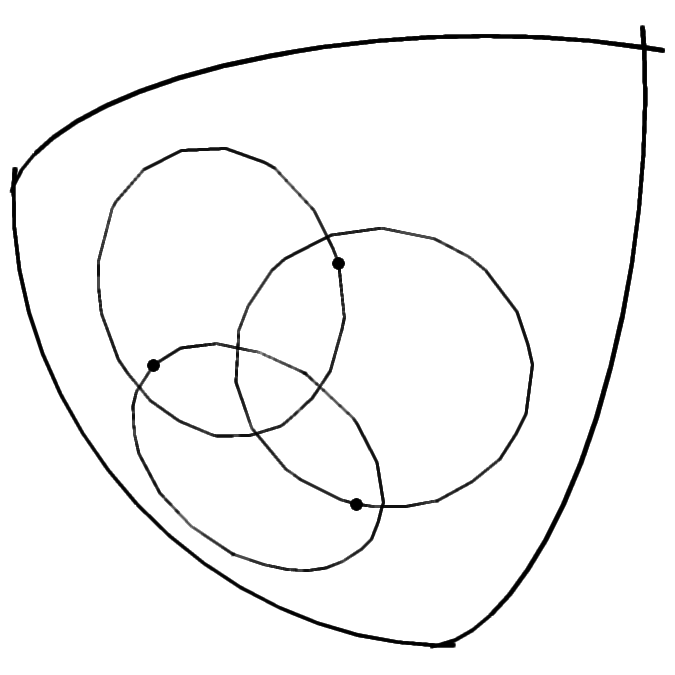
(a)

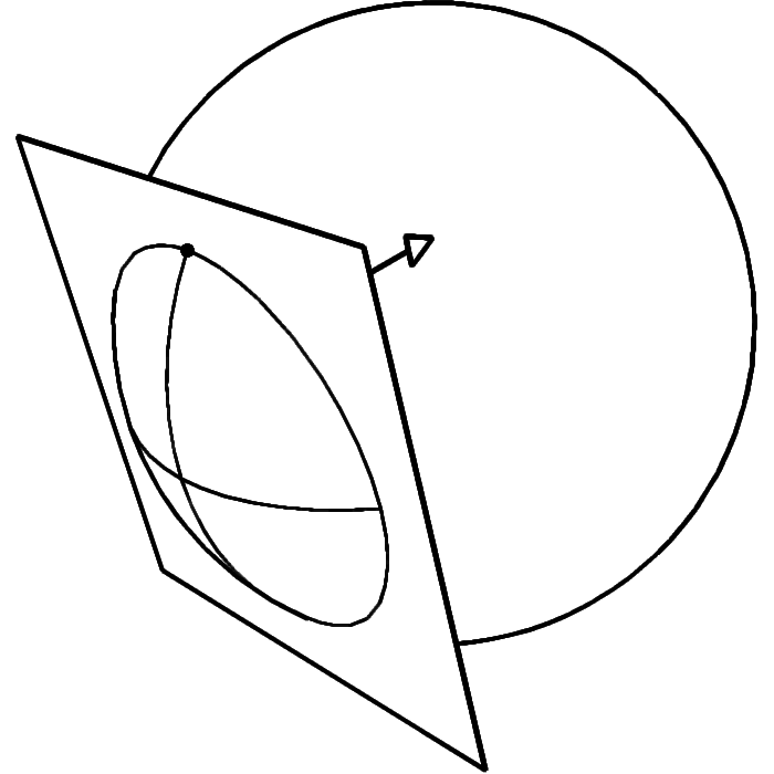
(b)

Figure 7: A 3-cycle embedded on a sphere section, and a disc on a sphere.

Now, recall the first part of the reduction: we wish to transform an instance of planar 3-sat to an instance of vertex cover in an associated undirected gadget graph. Our gadget graph is based upon a network used by Wang and Kuo [31] to prove the hardness of maximum independent set in undirected unit-disc graphs. However, we are able to simplify their non-planar network by using an instance of planar 3-sat rather than the general 3-sat. This simplification will be useful when implementing the second part of the reduction.

Let $\varphi$ be an instance of planar 3-sat with variables $u_{1},\,\dotsc,\,u_{n}$ and clauses $C_{1},\,\dotsc,\,C_{m}$. Recall that $\varphi$ is planar if the bipartite graph $H_{\varphi}$ consisting of a vertex for each variable, a vertex for each clause, and edges connecting each clause to its three variables, is planar. The associated, undirected, gadget graph $G_{\varphi}$ is constructed as shown in Figure 8. For each clause $C=(u_{i}\vee u_{j}\vee u_{k})$, add a $3$-cycle to the graph whose vertices are labelled by the appropriate literals for the variables $u_{i}$, $u_{j}$ and $u_{k}$. We call these the clause gadgets. For each variable $u_{i}$, add a large cycle of even length whose vertices are alternatingly labelled as the literals $u_{i}$ and $\bar{u}_{i}$. We call these the variable gadgets. Finally, add an edge from each variable in the clause gadgets to some vertex on the corresponding variable gadget with the opposite label – we choose a different variable vertex for each clause it is contained in.

Figure 8: The gadget graph $G_{\varphi}$ for $\varphi=(\bar{u}_{1}\vee u_{2}\vee u_{3})\wedge(u_{1}\vee\bar{u}_{2}\vee u_{3})$.

The next lemma is equivalent to the result shown by Wang and Kuo [31].

Lemma 4.2

[31] The planar 3-sat instance $\varphi$ is satisfiable if and only if $G_{\varphi}$ has vertex cover set of size at most $2m+\frac{1}{2}\sum_{i=1}^{n}{r_{i}}$, where $r_{i}$ is the number of vertices in the variable gadget’s cycle for $u_{i}$.

Proof

Suppose $\varphi$ is satisfiable. Take any satisfying assignment, and let $U$ be the set of literals which take true values in the assignment, $i.e.$ the literal “$u_{i}$” if the variable $u_{i}$ was assigned true, and the literal “$\bar{u}_{i}$” if the variable $u_{i}$ was assigned false. Let $\bar{U}$ be the remaining literals. Now, every vertex in a variable gadget of $G_{\varphi}$ whose label is in $\bar{U}$ will be selected to be in the vertex cover. In total this amounts to $\frac{1}{2}\sum_{i=1}^{n}{r_{i}}$ vertices, and these cover every edge in the variable gadgets of $G_{\varphi}$. Next consider the clause gadgets of $G_{\varphi}$. We must select two vertices of each clause gadget to cover the edges of the $3$-cycle. This amounts to $2m$ vertices. Since we have a satisfying assignment and we chose the nodes corresponding to $\bar{U}$ in the variable gadgets, each clause gadget must have at least one incident edge covered by the variable gadgets’ selected vertices. Hence, selecting the other two vertices will cover all incident edges to the clause gadgets, and all edges of the gadget’s cycle. Thus we have a vertex cover with $2m+\frac{1}{2}\sum_{i=1}^{n}{r_{i}}$ nodes. For example, in Figure 8, if we set all variables to false, one possible vertex cover is the set of vertices labelled with non-negated literals, $i.e.$ those coloured in white. (Note, clearly, the set of white vertices will not typically form a vertex cover in the gadget graph.)

Conversely, suppose we have a vertex cover $\mathcal{C}$ containing at most $2m+\sum_{i=1}^{n}\tfrac{r_{i}}{2}$ vertices. Each variable gadget must contribute at least $\tfrac{r_{i}}{2}$ vertices, otherwise we cannot cover every edge in its cycle. Each clause gadget must contribute at least two vertices, or one edge in the $3$-cycle will be uncovered. Hence, $\mathcal{C}$ contains exactly $2m+\sum_{i=1}^{n}\tfrac{r_{i}}{2}$ vertices. The $\frac{1}{2}r_{i}$ vertices from the variable gadget for $u_{i}$ corresponds either to the set of all vertices with negated labels or to the set with non-negated labels, otherwise there is an uncovered edge in the cycle. This induces a truth assignment; set $u_{i}$ to true if all the “$\bar{u}_{i}$”-labelled vertices are selected, and false if the “$u_{i}$”-labelled vertices are selected. Furthermore this is a satisfying assignment. To see this note that as $\mathcal{C}$ covers all edges, the unselected vertex in each clause is a literal which evaluates to true by the selected assignment. ∎

Hence, to solve for the satisfiability of $\varphi$, it suffices to test whether $G_{\varphi}$ admits a vertex cover with at most $2m+\tfrac{1}{2}\sum_{i=1}^{n}r_{i}$ vertices. It remains to show the second of the three parts of the reduction. That is, we need to show that this vertex cover problem in the undirected gadget graph can be solved by finding a minimum directed feedback vertex set in an oriented-disc graph $D_{\varphi}$. The basic idea is straightforward (albeit that the implementation is intricate). The oriented-disc graph $D_{\varphi}$ will contain a digon for each edge in some $G_{\varphi}$. However, it will also contain a collection of additional arcs. The key fact will be that these additional arcs form an acyclic subgraph of $D_{\varphi}$. Thus every cycle in $D_{\varphi}$ must induce a digon. Consequently, a minimum directed feedback vertex set need only intersect each digon to ensure that every cycle is hit. As argued previously, hitting the underlying graph formed by the digons of $D_{\varphi}$ corresponds to selecting a vertex cover in $G_{\varphi}$, as desired. We now formalise this argument.

Lemma 4.3

For every instance $\varphi$ of planar 3-sat, there exists an oriented-disc graph $D_{\varphi}$ on which the directed feedback vertex set problem is equivalent to the vertex cover problem on $G_{\varphi}$.

Proof

We prove this by explicitly constructing the oriented-disc drawing. Recall the disc graph $D_{\varphi}$ should contain a digon for each edge in $G_{\varphi}$. To do this, we begin with sufficiently a large planar drawing of $H_{\varphi}$, the planar bipartite network associated with $\varphi$. At each clause vertex, we place an oriented-disc construction for the clause gadget. This construction, along with its resulting graph, is shown in Figure 11. The figure shows a clause gadget and a section of each of the neighbouring three variable gadgets to which it is attached. Observe from the figure that, as claimed, the set of arcs created in $D_{\varphi}$ which are not in a digon, form an acyclic subgraph of $D_{\varphi}$.

Figure 9: Oriented-disc construction of the clause gadget, and its resulting graph.

(a)

(b)

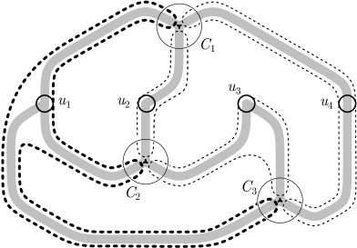
Figure 10: Paths of bidirected edges as oriented-disc drawings.

Figure 11: $G_{\varphi}$ as an oriented-disc graph.

It remains to construct the large cycles for the variable gadgets, and connect them to the clause gadgets. However, parts of these cycles are already included in the clause gadgets. Thus, it suffices to join these cycle segments together via paths of digons. This can be done via the oriented disc constructions shown in Figure 11. To draw the cycle for some variable, say $u_{i}$, we note that $u_{i}$’s vertex in the planar network $H_{\varphi}$ shares and edge with every clause gadget which connects to $u_{i}$’s gadget. Hence, as illustrated in Figure 11, we may follow along the edges of $H_{\varphi}$ to construct the cycle. For example, in the figure, the variable cycle for $u_{1}$ (highlighted) follows the topology of the edges incident to $u_{1}$’s vertex, and joins the clause gadgets (circled) to one another.

Observe that constructions in Figure 11 produce paths of digons in $D_{\varphi}$, where every arc produced is contained in a digon. It follows that the only arcs in $D_{\varphi}$ that are not in digons are in the neighbourhoods of the clause gadgets and, as we have seen, these are acyclic. But then, to hit all the cycles in $D_{\varphi}$, it suffices to hit all the digons, which, in turn, corresponds to a vertex cover in $G_{\varphi}$, completing the proof. ∎

This completes all the steps in the reduction and we obtain:

Theorem 4.1

The consumer rationality problem is NP-complete for a market with at least 3 commodities. ∎

References

- [1] S. Afriat, “The construction of a utility function from expenditure data”, International Economic Review, 8, pp67–77, 1967.
- [2] S. Afriat, “On a system of inequalities in demand analysis: an extension of the classical method”, International Economic Review, 14, pp460-472, 1967.
- [3] J. Apesteguia and M. Ballester, “A measure of rationality and welfare”, to appear in Journal of Political Economy, 2015.
- [4] C. Berge, “Färbung von Graphen deren sämtliche beziehungsweise deren ungerade Kreise starr sind (Zusammenfassung)”, Wiss. Z. Martin-Luther-Univ. Halle-Wittenberg Math.-Natur. Reihe, 10, pp114-115, 1961.
- [5] M. Chudnovsky, N. Robertson, P. Seymour and R. Thomas. “The strong perfect graph theorem”, Annals of Mathematics, pp51–229, 2006.
- [6] M. Dean and D. Martin, “Measuring rationality with the minimum cost of revealed preference violations”, to appear in Review of Economics and Statistics, 2015.
- [7] R. Deb and M. Pai, “The geometry of revealed preference”, Journal of Mathematical Economics, 50, pp203–207, 2014.
- [8] I. Dinur and S. Safra, “On the hardness of approximating minimum vertex cover”, Annals of Mathematics, 162(1), pp439-485, 2005.
- [9] Earl, R. (2007). Geometry II: 3.1 Stereographic Projection and the Riemann Sphere. Retrieved from https://people.maths.ox.ac.uk/earl/G2-lecture5.pdf
- [10] F. Echenique, S. Lee and M. Shum, “The money pump as a measure of revealed preference violations”, Journal of Political Economy, 119(6), pp1201–1223, 2011.
- [11] J. Gross, “Testing data for consistency with revealed preference”, The Review of Economics and Statistics, 77(4), pp701–710, 1995.
- [12] M. Grötschel, L. Lovász and A. Schrijver, “Polynomial algorithms for perfect graphs”, Annals of Discrete Mathematics, 21, pp325-356, 1984.
- [13] M. Grötschel, L. Lovász and A. Schrijver, Geometric Algorithms and Combinatorial Optimisation, Springer–Verlag, 1988.
- [14] V. Guruswami, J. Hastad, R. Manokaran, P. Raghavendra, and M. Charikar, “Beating the random ordering is hard: Every ordering CSP is approximation resistant”, SIAM J. Computing, 40(3), pp878–914, 2011.
- [15] M. Famulari, “A household-based, nonparametric test of demand theory”, Review of Economics and Statistics, 77, pp372-383, 1995.
- [16] J. Heufer, “A geometric approach to revealed preference via Hamiltonian cycles”, Theory and Decision, 76(3), pp329–341, 2014.
- [17] H. Houthakker, “Revealed preference and the utility function”, Economica, New Series, 17(66), pp159–174, 1950.
- [18] M. Houtman and J. Maks, “Determining all maximal data subsets consistent with revealed preference”, Kwantitatieve Methoden, 19, pp89–104, 1950.
- [19] R. Karp, “Reducibility among combinatorial problems”, Complexity of Computer Computations, New York: Plenum, pp85–103, 1972.
- [20] S. Khot, “On the power of unique 2-prover 1-round games”, Proceedings of STOC, pp767–775, 2002.
- [21] A. Koo, “An emphirical test of revealed preference theory”, Econometrica, 31(4), pp646–664, 1963.
- [22] L. Lovász, “Normal hypergraphs and the perfect graph conjecture”, discrete Mathematics, 2(3), pp253–267, 1972.
- [23] H. Rose. “Consistency of preference: the two-commodity case”, Review of Economic Studies, 25, pp124–125, 1958.
- [24] P. Samuelson, “A note on the pure theory of consumer’s behavior”, Economica, 5(17), pp61–71, 1938.
- [25] P. Samuelson, “Consumption theory in terms of revealed preference”, Economica, 15(60), pp243–253, 1948.
- [26] P. Seymour, “Packing directed circuits fractionally”, Combinatorica, 15(2), pp281–288, 1995.
- [27] O. Svensson, “Hardness of vertex deletion and project scheduling”, In Approximation, Randomization, and Combinatorial Optimization. Algorithms and Techniques, volume 7408 of Lecture Notes in Computer Science, pages 301–312. 2012.
- [28] J. Swafford and G. Whitney, “Nonparametric test of utility maximization and weak separability for consumption, leisure and money”, Review of Economics and Statistics, 69, pp458-464, 1987.
- [29] H. Varian, “Revealed preference”, in M. Szenberg et al. (eds.), Samulesonian Economics and the st Century, pp99–115, Oxford University Press, 2005.
- [30] H. Varian, “Goodness-of-fit in optimizing models”, Journal of Econometrics, 46, pp125-140, 1990.
- [31] D. Wang and Y. Kuo, “A study on two geometric location problems”, Information Processing Letters, 28(6), pp281–286, 1988.