Probing the isotropy of cosmic acceleration
traced by Type Ia supernovae
Abstract
We present a method to test the isotropy of the magnitude-redshift relation of Type Ia Supernovae (SNe Ia) and single out the most discrepant direction (in terms of the signal-to-noise ratio) with respect to the all-sky data. Our technique accounts for possible directional variations of the corrections for SNe Ia and yields all-sky maps of the best-fit cosmological parameters with arbitrary angular resolution. To show its potential, we apply our method to the recent Union2.1 compilation, building maps with three different angular resolutions. We use a Monte Carlo method to estimate the statistical significance with which we could reject the null hypothesis that the magnitude-redshift relation is isotropic based on the properties of the observed most discrepant directions. We find that, based on pure signal-to-noise arguments, the null hypothesis cannot be rejected at any meaningful confidence level. However, if we also consider that the strongest deviations in the Union2.1 sample closely align with the dipole temperature anisotropy of the cosmic microwave background, we find that the null hypothesis should be rejected at the per cent confidence level, slightly depending on the angular resolution of the study. If this result is not due to a statistical fluke, it might either indicate that the SN data have not been cleaned from all possible systematics or even point towards new physics. We finally discuss future perspectives in the field for achieving larger and more uniform data sets that will vastly improve the quality of the results and optimally exploit our method.
Subject headings:
cosmology:dark energy, supernovae:general, methods:data analysis.1. Introduction
In 1998, the luminosity-redshift relation (Hubble diagram) of a few tens of Type Ia supernovae (SNe) provided the evidence base for the accelerated expansion of the universe (Riess et al., 1998; Perlmutter et al., 1999). Since then, major efforts have been made to increase the sample size, extend it to higher redshift, and refine the observational and data-reduction techniques. Current datasets already include several hundreds of objects but the quest for dark energy drives copious activity in this field.
The control of systematic errors is the key to making the study of SNe Ia a prime cosmological tool. Suzuki et al. (2012) state that systematic uncertainties already dominate over the statistical ones in the determination of the cosmological parameters. Given that systematics will become even more important in the future, a careful scrutiny of all the possible sources of methodological bias is crucial. In this paper, we focus on the spatial isotropy of the Hubble diagram traced by type Ia SNe. The standard cosmological model is rooted in the assumption that the Universe is homogeneous and isotropic on large scales. Hence, SNe Ia are expected to (statistically) obey the same dimming relation in all directions. There are, however, several phenomena that could introduce anisotropies with different characteristic scales and amplitudes in the observed expansion rate. To name a few: dust absorption (both in the Milky Way and in the galaxies hosting the SNe), redshift-space distortions due to large-scale motions, weak gravitational lensing, the presence of large-scale structures and contamination of the SNe Ia samples. Detecting these effects and correcting for them would ultimately lead to tighter and less biased constraints on the cosmological parameters.
At the same time, it is healthy to scrutinise the validity of the standard model of cosmology (Kroupa, 2012; Kroupa et al., 2012; Kroupa, 2015; Koyama, 2015) and its fundamental assumptions, namely those of the cosmological principle. Ruling out cosmic isotropy with high statistical confidence would lead to a major paradigm shift especially if such a conclusion is confirmed by multiple datasets affected by different systematics. In this respect, the analysis of temperature anisotropies in the Cosmic Microwave Background (CMB) has dominated the scene in the last decade. The WMAP satellite detected a few large-scale “anomalies” that somewhat deviate from the expectations of the standard model that best fits the data on smaller scales (Tegmark et al., 2003; Eriksen et al., 2004; Hansen et al., 2009; Copi et al., 2010a). In brief, the quadrupole and octopole terms are surprisingly planar and there is a significant alignment between them. Moreover, their normals lie close to the axis of the CMB dipole. This discovery generated a long lasting debate in the literature concerning whether or not these features are genuine signs of new physics.
Alternatively they could be due to the influence of data processing, to the imperfect removal of foreground contaminants and secondary astrophysical effects (Rassat et al., 2014), as well as to a statistical fluke (Bennett et al., 2011). The Planck satellite recently confirmed the existence of these alignments (Planck Collaboration et al., 2014b) suggesting that they are not artifacts of the data-reduction pipelines. A satisfactory explanation for the origin of these asymmetries is still not available.
The isotropy of the Hubble diagram for SNe Ia has been repeatedly tested. Kolatt & Lahav (2001) used 79 SNe from Riess et al. (1998) and Perlmutter et al. (1999) to perform localized fits within an opening angle of around random directions. After expanding the best-fitting cosmological parameters in low multipoles, they found that no dipole anisotropy was statistically significant. Subsequent studies mainly adopted two methods: either they compared Hubble diagrams for pairs of hemispheres and looked for the most discrepant hemispheric cut (Hemispherical Comparison, e.g. Schwarz & Weinhorst, 2007) or fit a dipole angular distribution (Dipole Modulation Fitting, e.g. Cooke & Lynden-Bell, 2010). Other authors looked for angular correlations in SN magnitudes (Blomqvist et al., 2008) or analyzed the magnitude-redshift relation in the context of anisotropic cosmological models (Koivisto & Mota, 2008; Campanelli et al., 2011). Low-redshift samples were used to estimate the direction and amplitude of the local bulk flow (Bonvin et al., 2006; Schwarz & Weinhorst, 2007; Colin et al., 2011; Turnbull et al., 2012; Rathaus et al., 2013; Feindt et al., 2013; Kalus et al., 2013; Appleby & Shafieloo, 2014; Appleby et al., 2015). At the same time, several authors analysed higher-redshift data to look for large-scale anisotropies (Schwarz & Weinhorst, 2007; Gupta & Saini, 2010; Cooke & Lynden-Bell, 2010; Antoniou & Perivolaropoulos, 2010; Mariano & Perivolaropoulos, 2012; Cai et al., 2013; Li et al., 2013; Campanelli et al., 2011; Zhao et al., 2013; Heneka et al., 2014; Wang & Wang, 2014; Yang et al., 2014; Chang & Lin, 2015; Jiménez et al., 2015), which is also the aim of our work. Statistically significant deviations have been detected at low redshift (Schwarz & Weinhorst, 2007), while no high-redshift study could rule out isotropy at more than 2 Gaussian standard deviations, .
In this paper, we present a simple but powerful method to test the isotropy of the luminosity-redshift relation for SNe Ia. Contrary to most previous studies, our analysis neither searches for hemispheric asymmetries and dipolar patterns nor does it use any other template anisotropic configuration. For each direction on the celestial sphere , we derive a set of cosmological parameters by considering only the SNe that lie within an angle from . We then build maps of these “local cosmological parameters” with different values of and identify the directions associated with the most significant anisotropies taking into account that the number of datapoints used in the fit fluctuates from one direction to another. For completeness, we consider that the correction for the distance modulus of SNe Ia might also depend on due, for instance, to dust extinction. Therefore, our strategy is able to detect anisotropies generated both by physical effects and by systematics. Even though our method is best suited for the large SN samples with nearly uniform sky distribution that will become available in the next decade, we provide an example of its potential by applying it to the Union2.1 SN Ia compilation (Suzuki et al., 2012) from the Supernova Cosmology Project (SCP). We limit our study to redshifts in order to minimize the influence of local inhomogeneities and bulk flows.
The rest of this paper is organised as follows. Section 2 describes the main properties of the Union2.1 sample. Our method of analysis is introduced in Section 3. Results are presented and critically discussed in Section 4. Finally, we conclude in Section 5.
2. Data
The Union2.1 compilation (Suzuki et al., 2012) collects data for 580 SNe Ia in the redshift range of . It combines entries from 19 datasets uniformly analysed after adopting strict lightcurve quality cuts and the SALT2 lightcurve-fitter (Guy et al., 2007). The Union2.1 catalog has been built for dark-energy science and updates the previously released Union (Kowalski et al., 2008) and Union2 (Amanullah et al., 2010) compilations. In particular, it contains 14 new SNe discovered in the HST Cluster Supernova Survey (a survey run by the SCP) that pass the Union2 selection cuts. Ten of these SNe are at which makes the Union2.1 sample ideal for studying isotropy out to the largest possible distances.
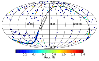
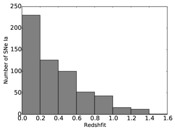
The Union2.1 catalog provides five entries for each SN, specifically: name, redshift (CMB centric), distance modulus, error in the estimate of the distance modulus, and the probability that the SN was hosted by a low-mass galaxy. We obtained the coordinates for all the SNe Ia in the compilation either from the NASA/IPAC Extragalactic Database (NED)111The NASA/IPAC Extragalactic Database (NED) is operated by the Jet Propulsion Laboratory, California Institute of Technology, under contract with the National Aeronautics and Space Administration. or directly from the SuperNova Legacy Survey (SNLS) data release (Astier et al., 2006). The sky distribution of Union2.1 SNe is plotted in Figure 1. The angular position of each SN is marked by a symbol which has been colour-coded based on redshift. Several features are immediately apparent in the image. First, there are only a few SNe close to the galactic plane. Second, an arc-like region in the southern hemisphere is much more densely populated than the rest. This is the footprint of the Sloan Digital Sky Survey-II (SDSS-II) SN search and corresponds to the southern equatiorial stripe (Stripe 82, with coordinates and ) which has been imaged repeatedly with broad wavelength coverage and also been subject to extensive spectroscopic studies (Kessler et al., 2009). Finally, high-redshift SNe are very sparsely distributed and rare which is also evident from the redshift distribution of the Union2.1 SNe shown in Figure 2.
3. Method
As mentioned in the Introduction, previous studies on the isotropy of the luminosity-redshift relation of SNe Ia have mainly searched for dipolar anisotropies or hemispheric asymmetries. In this section, we introduce a more general method that does not assume any particular form of the anisotropy.
3.1. Cone Analysis
Let us consider a particular direction on the sky, , with Galactic longitude and latitude . In order to single out a finite region surrounding , we consider a cone with apex angle subtending a solid angle of sr on the celestial sphere. The apex of the cone is located at the centre of the Galactic coordinate system and its axis of symmetry points towards . After isolating the SNe Ia contained within the cone, we build their magnitude-redshift relation and derive “local cosmological parameters” by fitting a theoretical relationship to it (see Section 3.2 for details). We then vary the cone direction making sure that we cover the whole sky. For convenience, we move along the pixel centers of a HEALPix222Hierarchical Equal Area isoLatitude Pixelization, http://healpix.sourceforge.net grid (Górski et al., 2005).
For the application of the method to the Union2.1 data, we repeat the analysis using three different opening angles: (hemispheres), and . We use a HEALPix grid with 192 pixels so that the solid angle subtended by each pixel is much smaller than that subtended by the cones.
3.2. Formulation
3.2.1 Global fit
SNe Ia are not perfect standard candles, their peak brightness correlates with their color, the light-curve width and the mass of the host galaxy. In the Union2.1 sample, individual lightcurves are analyzed with the SALT2 fitter which provides estimates for three parameters: the peak magnitude, , in the rest-frame B band, the deviation, , from the average light-curve shape and the deviation, , from the mean color. The color and light-curve-shape corrected distance modulus is then written in terms of four unknown parameters ( and ) so that
| (1) |
where is the absolute B-band magnitude at maximum of a SN Ia and denotes the probability that the SN Ia is hosted by a galaxy with stellar mass . This probability is estimated differently for untargeted and targeted surveys.
In the context of the theory of general relativity, homogeneous and isotropic universes are described by Friedmann-Lemaître-Robertson-Walker models. For simplicity we only consider flat models in which the density parameters for the matter and the cosmological constant satisfy the relation . Following standard practice, we write the magnitude-redshift relation of SNe Ia in terms of the distance modulus
| (2) |
where
| (3) |
is the dimensionless “Hubble-constant-free” luminosity distance and is the Hubble radius defined in terms of the speed of light and the present-day value of the Hubble constant.
Classically, the SN data are fitted with a cosmological model assuming Gaussian errors and following a maximum likelihood approach (e.g. Astier et al., 2006). For Type Ia SNe, this corresponds to minimising the target function
| (4) |
where is a -dimensional vector with elements and is the covariance matrix of the errors in the observed distance moduli. For the Union compilations, this matrix is publicly available. Its off-diagonal elements include several contributions due to the light-curve fits, galactic extinction, gravitational lensing, peculiar velocities and sample-dependent systematics. The nuisance parameters and are fitted simultaneously with the cosmological parameters. Actually, the best-fit values for and are completely degenerate as only the combination appears in eq. (4). Using the whole data set gives the following best-fit values (Suzuki et al., 2012) , , , and (for km s-1Mpc-1).
3.2.2 Local fits
The parameters and describe correlations between different SN observables and might vary for the different surveys of a compilation. Karpenka et al. (2015) found inconsistencies between the values of these correction parameters in the Union2 catalog. In order to account for possible direction-dependent systematics, when we consider localized sub-samples of the Union2.1 data, we should in principle allow them to vary freely. However, this would require knowledge of the covariance between , and for individual SNe. Regrettably this information is not provided in the Union2.1 catalog. We therefore adopt a simplified approach by assuming a constant correction, , for the distant modulus of all the SNe lying within a cone. In other words, we keep the quantities and fixed at their global best-fit value (hereafter denoted with a hat) but we write
| (5) |
with . Note that accounts for both an “anisotropic Hubble constant” and for the mean effect of variations in and due to systematic errors. We are left with a two-dimensional problem. For each pixel on the sky, we then determine the best-fitting values of the cosmological parameter and of the correction parameter by minimizing the target function (covariances are extracted from after identifying the SNe in the cone). However, the model parameters anticorrelate: directions associated with large values of provide low values of (and viceversa). In order to minimise this effect, we use the luminosity distance, , evaluated at the mean redshift of the sample () as a pivot point and define
| (6) |
where and are our free parameters.
4. Results
4.1. All-sky fit
To test the consistency of our approach with previous studies, we first perform an all-sky fit. Results are shown in Table 1 for the entire Union2.1 sample and for two sub-sets including the SNe Ia with redshift smaller and larger than (in this paper, uncertainties on the value of single parameters always correspond to ). Our results are in excellent agreement with the analysis in Suzuki et al. (2012) who found (see their Table 7). Also note that setting , km s-1Mpc-1 and corresponds to mag which gives mag for and .
| (mag) | |||
|---|---|---|---|
| All SNe | 0.94 | ||
| 0.94 | |||
| 0.93 |
4.2. Cone analysis
4.2.1 maps
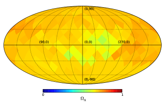
Sky maps of the best-fit values for (left) and (right) are shown in Figure 3 for three different cone opening angles (from top to bottom: , and radians). These have been obtained using all the Union2.1 SNe with redshift . White pixels indicate the directions (mostly located around the Galactic equator) in which the corresponding cone contains less than SNe Ia. These directions are excluded from all statistical analyses because they are associated with extremely large errors in the fitted parameters. Of course their number increases with decreasing the opening angle of the sampling cone. Similarly, the size of fluctuations in the best-fit values for and increases with reducing .
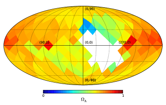
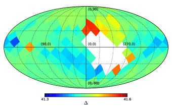
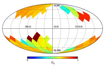
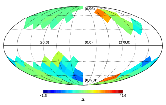
4.2.2 Most discrepant directions
Although Figure 3 gives a first visual impression of the local best-fit parameters, it does not take into account the non-uniform sky coverage of the Union2.1 data set. For a given opening angle, different directions on the celestial sphere are generally associated with very different numbers of SNe Ia. This strongly influences the uncertainty of the best-fit values.
In order to single out the most discrepant directions in a statistically meaningful way, we assume the null hypothesis that the Universe follows the cosmological principle and there are no angle-dependent systematic effects plaguing the Union2.1 sample. For each pixel we then evaluate the target function fixing the free parameters at the values and that provide the best-fit solution for the complete Union2.1 sample. However, only the SNe within the sampling cone are used to calculate the value that we denote by . Finally, we estimate the probability that random noise could generate a value exceeding . Assuming Gaussian errors, this probability coincides with the cumulative chi-square distribution function evaluated at :
| (7) |
where is the number of degrees of freedom – i.e. the number of SNe Ia used in the fitting procedure minus two (the number of free parameters). We adopt the value as a measure of how well the all-SNe best-fit parameters also describe the SN data in a specific direction on the sky. Consequently we identify the most discrepant direction (i.e. the direction showing the most statistically significant deviation from isotropy) with the pixel showing the smallest value. It is worth stressing that this is not necessarily the direction in which the Universe (or the SN data) might present the strongest intrinsic anisotropy but only the direction in which, given the current data, we can measure the most meaningful deviation in terms of the signal-to-noise ratio.
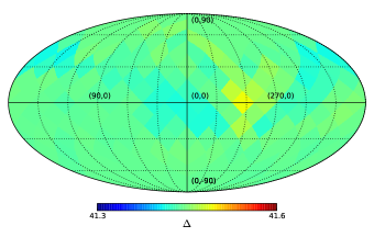
Maps of the value are plotted in Fig. 4 for the three different cone opening angles. The most (second-most) discrepant directions are highlighted with a star (circle) in each panel. Further information is provided in Table 2 which gives the value, the coordinates and the number of SNe Ia associated with the most and the second-most discrepant directions together with the local best-fit parameters. The motivation for showing two directions per map is as follows: i) the difference between their -values is small (see Table 2), ii) the covariance matrix provided by the SCP is likely to be a noisy estimate, and iii) neglecting off-diagonal covariances switches the order between these directions for .
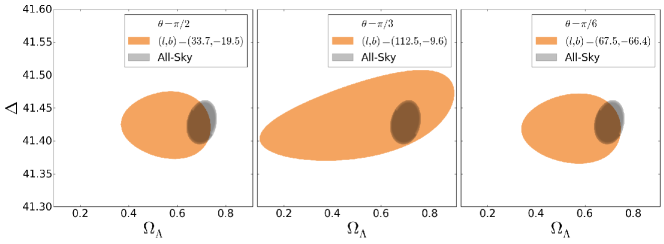
Intriguingly, the most discrepant directions obtained with the three cone opening angles lie close to each other. Also the best-fit parameters are quite similar (let us not forget, however, that the maps with different are not independent as they use the same SNe and that there is significant overlap between the most discrepant cones). In Figure 5 we compare the formal333I.e. obtained assuming independent Gaussian errors. The limitation of this approach is discussed in detail in Section 4.2.3. confidence regions () obtained from the all-SNe fit against those derived from the local fits along the most discrepant directions. In all cases, the tension between the local and the global fits is marginal and the formal regions always overlap.
Visual inspection of Figure 4 shows a striking contrast between the values measured in the Northern and the Southern Galactic Hemispheres (hereafter NGH and SGH, respectively), although there is no tension between the luminosity-distance relation in the two hemispheres (see Table 3). The discrepancy in the values is mainly due to the fact that the Union2.1 uncertainties in the distance-moduli are on average 30 per cent larger in the NGH. Consequently, the reduced chi-square tends to be smaller in the NGH although there are many more SNe in the SGH (227 vs 123) to drive the fit results for SNe with closer to the SGH results.
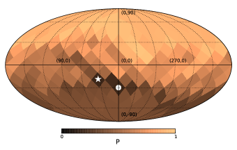
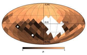
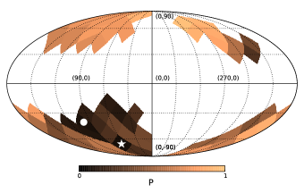
| (33.7,-19.5) | 1.09 | 0.192 | 128 | |||
| (0.0,-30.0) | 1.08 | 0.197 | 161 | |||
| (112.5,-9.6) | 1.20 | 0.086 | 74 | |||
| (56.2,-41.8) | 1.15 | 0.101 | 118 | |||
| (67.5,-66.4) | 1.18 | 0.081 | 100 | |||
| (101.2,-41.8) | 1.20 | 0.085 | 73 |
| N | |||||
|---|---|---|---|---|---|
| NGH | 0.82 | 123 | 0.30 | ||
| SGH | 1.01 | 227 | 0.23 |
4.2.3 Monte Carlo analysis
Taken at face value, the probabilities associated with most discrepant directions (see Table 2) are moderately significant. However, assuming Gaussian errors is a strong limiting factor. Also, the size of the errorbars in the distance modulus (and the off-diagonal covariances) provided in the Union2.1 catalog might be inaccurate and, as a consequence, inference based on the statistic might be biased. For these reasons, we re-evaluate the statistical significance of the anisotropies using a more robust Monte Carlo method.
In order to assess the impact of random errors and account for the non-uniform angular distribution of the Union2.1 sample, we build 1000 mock catalogs by randomly shuffling the distance moduli of the Union2.1 SNe. In practice, we assign the distance modulus, its uncertainty and the redshift of a SN Ia to the angular position of another (random) SN Ia. Each mock catalog thus contains exactly the same number of SNe as the original Union2.1 sample and has exactly the same SN sky distribution. Moreover, all possible anisotropies should be erased by the shuffling procedure while the statistical properties of the distance moduli and their uncertainties are unchanged with respect to the observational data. Therefore our mock catalogs form an ensemble of realizations mimicking an isotropic Universe but having the same statistical properties as the actual Union2.1 data.
We treat the mock catalogs as the real data and identify the two most discrepant directions in each of them using the -value-based method for the three different cone opening angles. We then compute the fraction, , of the realizations in which the most (or the second most) discrepant direction is associated with a value which is smaller than the observed ones reported in Table 2. For the most (second-most) discrepant directions we find that and (0.473, 0.550, 0.490) for , and , respectively. Purely based on this signal-to-noise criterion, we conclude that no statistically significant anisotropy can be detected in the Union2.1 sample.
4.2.4 Alignment with the CMB dipole
Although the Monte Carlo test shows that random chance in an isotropic universe can easily produce most discrepant directions with lower values than we found analyzing the actual data, the observed anisotropies present a characteristic feature which is worth being discussed.
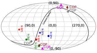
The temperature distribution in the CMB presents a strong dipole anisotropy which is usually interpreted as due to our motion with respect to the CMB rest frame towards the direction with Galactic coordinates (Planck Collaboration et al., 2014a). Figure 6 shows that the most discrepant directions we obtained from the Union2.1 sample closely align with the axis of the CMB dipole (CDP) in the SGH opposite to our motion with respect to the CMB rest frame (hereafter CDP-South). Assuming that the redshifts of the SNe Ia in the Union2.1 compilation have been correctly transformed to the CMB rest frame, there is no obvious reason for explaining the origin of this alignment. As already mentioned in the Introduction, the CMB quadrupole (CQP) and octopole (COP) are also closely aligned with the CDP (Planck Collaboration et al., 2014b; Schwarz et al., 2004; Copi et al., 2010b, 2013, see Figure 6). It is yet unclear whether these alignments are a statistical fluke or a signature of new physics. Anyway, our study shows that the magnitude-redshift relation of SNe Ia with tends to be different in the same direction (albeit the difference is detected with low signal-to-noise ratio). Other authors have reported similar results using the Union compilations (Cooke & Lynden-Bell, 2010; Antoniou & Perivolaropoulos, 2010; Li et al., 2013).
The debate on the physical relevance of the CMB anomalies opened up a discussion in the literature about the legitimacy and validity of “a posteriori” analyses in which tailored statistical tests are designed and hand picked after noticing the peculiarities in the data. A widespread point of view states that in a large dataset it is always possible to isolate some “strange” features (e.g. Bennett et al., 2011). To minimize the pitfalls of a posteriori reasoning, we focus on the well established CDP and do not consider the CQP and COP any further.
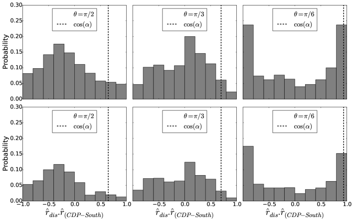
We thus proceed to quantify the probability that the most discrepant directions (defined in terms of the value as above) form a given angle with the CDP under the null hypothesis of an isotropic magnitude-redshift relation. In order to account for the non-uniform sky distribution of the Union2.1 sample (especially for the SDSS-II stripe which is close to the CDP-South) we use the Monte Carlo realizations introduced in Section 4.2.3. Figure 7 shows the resulting probability distribution for the cosine of the angle between the most discrepant direction and the axis of the CDP-South. Our measurements from the Union2.1 data are indicated by vertical dashed lines. The second column in Table 4 reports the fraction of Monte Carlo realisations, , showing a better alignment than our measurement. Our results suggest that it is rather unlikely to get an alignment as strong as the observed one under the null hypothesis of an isotropic magnitude-redshift relation. In fact, considering the most discrepant direction for , only 8.5 per cent of the Monte Carlo realisations show a smaller separation angle than observed and this reduces to 4.5 percent for . Note that for and , the second-most discrepant directions are even better aligned with CDP-South. In these cases .
The test above is blind to the statistical significance of the most discrepant directions. In order to account for this, we compute the fraction of Monte Carlo realisations, , for which the most discrepant directions are at least as significant as the measured ones (in terms of the value) and are also better aligned with the CDP-South. The third column in Table 4 shows that for the most discrepant directions this probability is smaller than 4.5 percent for all the opening angles which means the null hypothesis of an isotropic magnitude-redshift relation should be rejected at the 95 per cent confidence level. The value of reduces to a fraction of a percent when considering the second-most discrepant direction for and .
The measured anisotropy could be due to a statistical fluke, to systematics in the SNe data (or error bars), to the presence of localized large scale structures, or even a sign of the failure of the cosmological principle. To further investigate its properties, we repeat the analysis along the most discrepant directions after slicing the SNe data in five redshift bins (, , , and ). Regrettably, due to the low number of SNe in each bin, the formal errors span most, if not all, the parameter space . Therefore no meaningful statements can be made regarding the variations of the best-fit cosmological parameters along the most-discrepant directions. In terms of signal-to-noise ratio, however, the redshift range clearly emerges as the most discrepant one for all the cone opening angles ( and for and , respectively).
Given the current sparsity of the data, no firm conclusion can be drawn except from the fact that there seems to be a moderately statistically significant (2-3) anisotropy in the magnitude-redshift relation of SNe Ia close to the direction opposite to our motion with respect to the CMB rest frame. It is worth remembering that, in the Union2.1 compilation, most of the SNe Ia surrounding the CDP-South come from the SDSS-II stripe. Further investigations are thus needed to clarify the relation between the CMB dipole axis, our motion, and the way SNe data around this direction are treated.
| 0.085 | 0.027 | ||
| 0.152 | 0.052 | ||
| 0.045 | 0.021 | ||
| 0.008 | 0.002 | ||
| 0.064 | 0.045 | ||
| 0.010 | 0.006 |
5. Conclusions and future perspectives
We presented a simple but powerful method for investigating the isotropy of cosmic acceleration traced by Type Ia SNe with different angular resolution, . The key idea is to consider all the SNe contained within a cone with vertex located at the origin of the Galactic coordinate system and with apex angle . “Local cosmological parameters” are derived by fitting the magnitude-redshift relation of the SNe in the cone with a theoretical relation. The cone direction is then changed so that to cover the entire sky. Our cone-analysis method takes into account the mean variation of the SNe Ia correction parameters over different directions, and yields all-sky maps of the best-fit cosmological parameters.
Although a large data set with a uniform sky distribution is required for a thorough investigation of isotropy, we provided an example of the potential of our method by applying it to the SNe Ia with redshift in the Union2.1 compilation. Assuming a flat Universe in the context of the standard cosmological model, we fitted the magnitude-redshift relation by varying the density parameter of the cosmological constant, , and a parameter , , including the effect of both the Hubble constant and the mean SNe Ia correction parameters. We used a HEALPix grid to discretise the celestial sphere and obtained sky maps for and considering three different cone-opening angles , and .
We ranked the pixels in each map in terms of a value derived from the distribution and which measures how much the local fits differ from the cosmology determined using the entire Union2.1 sample (in a signal-to-noise sense). We thus found the most discrepant directions (two per cone opening angle). Finally, we used a Monte Carlo method to estimate the statistical significance at which we could reject the null hypothesis that the magnitude-redshift relation of SNe Ia is isotropic based on the properties of the most discrepant directions. We found that random fluctuations can easily produce deviations from isotropy with smaller values than measured in the Union2.1 data. Therefore, the null hypothesis cannot be rejected at any meaningful confidence level based on signal-to-noise arguments alone. However, if we also consider that the detected anisotropies in the Union2.1 sample align well with CMB dipole axis in the Southern Galactic Hemisphere, we find that the null hypothesis should be rejected at the 97.3, 97.9 and 95.5 per cent confidence level for opening angles , and , respectively.
We conclude that, although the deviation from isotropy that we found is not very significant per se in terms of signal-to-noise ratio, its vicinity to the axis of the CMB dipole (which enters the pipeline to determine the SN redshift in the CMB rest frame) with 2-3 statistical significance requires further investigation both on the observational and on the theoretical sides. Note that other observations detected anisotropies in the same area of the sky. The statistical significance of the quadrupole–octopole alignment in the CMB is approximately 99 per cent (Planck Collaboration et al., 2014b). On combination of the likelihoods between the CMB and SN Ia, the null hypothesis of isotropy should be rejected at the 99.98 per cent confidence level (approximately 3.5 Gaussian ). In this paper we followed a conservative approach by only considering the SN Ia data.
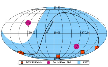
This study should be repeated when larger data sets with more uniform sky coverage will be available. Several major current and future facilities have dedicated plans for studying the accelerated expansion of the universe using SNe Ia. For instance, the Dark Energy Survey (DES) integrates a dedicated program that should detect around 4000 SNe Ia in the redshift range (Bernstein et al., 2012). Similarly, the Euclid mission includes a SNe survey within two deep fields each covering around 20 deg2 and is expected to discover about 3000 SNe Ia out to (Laureijs et al., 2011). However, both these surveys will only provide SN data in relatively small regions of the sky (see Figure 8) and the most promising perspective for isotropy tests of the Hubble diagram comes from the Large Synoptic Survey Telescope (LSST). While its use for a SN-dedicated survey on a limited area of sky will be able to deliver as many as SNe Ia (in 10 years) with very precisely measured light curves, in its normal operating mode (due to its rapid cadence), LSST will discover around SNe Ia per year in the redshift range and across a large fraction of the sky (Ivezic et al., 2008). Finally, the Panoramic Survey Telescope & Rapid Response System (Pan-STARRS, Brout et al., 2013) which is observing the Northern part of the sky will complement the above mentioned surveys. In summary, exciting perspectives to test the isotropy of the magnitude-redshift relation of SNe Ia with unprecedented accuracy will open up within the next two decades.
Acknowledgments
We thank the referee for providing constructive comments on the manuscript. BJ thanks Ryan Cooke for help with finding some of the SNe Ia coordinates, Dominik Schwarz and Marek Kowalski for constructive comments and Douglas Applegate for very useful discussions. BJ was supported through a stipend from the International Max Planck Research School (IMPRS) for Astronomy and Astrophysics at the Universities of Bonn and Cologne. CP acknowledges support from the Deutsche Forschungsgemeinschaft through the Transregio 33 “The Dark Universe”.
References
- Amanullah et al. (2010) Amanullah, R., Lidman, C., Rubin, D., et al. 2010, ApJ, 716, 712
- Antoniou & Perivolaropoulos (2010) Antoniou, I., & Perivolaropoulos, L. 2010, J. Cosmology Astropart. Phys, 12, 12
- Appleby & Shafieloo (2014) Appleby, S., & Shafieloo, A. 2014, J. Cosmology Astropart. Phys, 3, 7
- Appleby et al. (2015) Appleby, S., Shafieloo, A., & Johnson, A. 2015, ApJ, 801, 76
- Astier et al. (2006) Astier, P., Guy, J., Regnault, N., et al. 2006, A&A, 447, 31
- Bennett et al. (2011) Bennett, C. L., Hill, R. S., Hinshaw, G., et al. 2011, ApJS, 192, 17
- Bernstein et al. (2012) Bernstein, J. P., Kessler, R., Kuhlmann, S., et al. 2012, ApJ, 753, 152
- Blomqvist et al. (2008) Blomqvist, M., Mörtsell, E., & Nobili, S. 2008, J. Cosmology Astropart. Phys, 6, 27
- Bonvin et al. (2006) Bonvin, C., Durrer, R., & Kunz, M. 2006, Physical Review Letters, 96, 191302
- Brout et al. (2013) Brout, D., Scolnic, D., Rest, A., et al. 2013, in American Astronomical Society Meeting Abstracts, Vol. 221, American Astronomical Society Meeting Abstracts #221, 253.12
- Cai et al. (2013) Cai, R.-G., Ma, Y.-Z., Tang, B., & Tuo, Z.-L. 2013, Phys. Rev. D, 87, 123522
- Campanelli et al. (2011) Campanelli, L., Cea, P., Fogli, G. L., & Marrone, A. 2011, Phys. Rev. D, 83, 103503
- Chang & Lin (2015) Chang, Z., & Lin, H.-N. 2015, MNRAS, 446, 2952
- Colin et al. (2011) Colin, J., Mohayaee, R., Sarkar, S., & Shafieloo, A. 2011, MNRAS, 414, 264
- Cooke & Lynden-Bell (2010) Cooke, R., & Lynden-Bell, D. 2010, MNRAS, 401, 1409
- Copi et al. (2010a) Copi, C. J., Huterer, D., Schwarz, D. J., & Starkman, G. D. 2010a, Advances in Astronomy, 2010, 92
- Copi et al. (2010b) —. 2010b, Advances in Astronomy, 2010, arXiv:1004.5602
- Copi et al. (2013) —. 2013, ArXiv e-prints, arXiv:1311.4562
- Eriksen et al. (2004) Eriksen, H. K., Hansen, F. K., Banday, A. J., Górski, K. M., & Lilje, P. B. 2004, ApJ, 605, 14
- Feindt et al. (2013) Feindt, U., Kerschhaggl, M., Kowalski, M., et al. 2013, A&A, 560, A90
- Górski et al. (2005) Górski, K. M., Hivon, E., Banday, A. J., et al. 2005, ApJ, 622, 759
- Gupta & Saini (2010) Gupta, S., & Saini, T. D. 2010, MNRAS, 407, 651
- Guy et al. (2007) Guy, J., Astier, P., Baumont, S., & et al. 2007, A&A, 466, 11
- Hansen et al. (2009) Hansen, F. K., Banday, A. J., Górski, K. M., Eriksen, H. K., & Lilje, P. B. 2009, ApJ, 704, 1448
- Heneka et al. (2014) Heneka, C., Marra, V., & Amendola, L. 2014, MNRAS, 439, 1855
- Ivezic et al. (2008) Ivezic, Z., Tyson, J. A., Abel, B., et al. 2008, ArXiv e-prints, arXiv:0805.2366
- Jiménez et al. (2015) Jiménez, J. B., Salzano, V., & Lazkoz, R. 2015, Physics Letters B, 741, 168
- Kalus et al. (2013) Kalus, B., Schwarz, D. J., Seikel, M., & Wiegand, A. 2013, A&A, 553, A56
- Karpenka et al. (2015) Karpenka, N. V., Feroz, F., & Hobson, M. P. 2015, MNRAS, 449, 2405
- Kessler et al. (2009) Kessler, R., Becker, A. C., Cinabro, D., et al. 2009, ApJS, 185, 32
- Koivisto & Mota (2008) Koivisto, T., & Mota, D. F. 2008, ApJ, 679, 1
- Kolatt & Lahav (2001) Kolatt, T. S., & Lahav, O. 2001, MNRAS, 323, 859
- Kowalski et al. (2008) Kowalski, M., Rubin, D., Aldering, G., et al. 2008, ApJ, 686, 749
- Koyama (2015) Koyama, K. 2015, ArXiv e-prints, arXiv:1504.04623
- Kroupa (2012) Kroupa, P. 2012, PASA, 29, 395
- Kroupa (2015) —. 2015, Canadian Journal of Physics, 93, 169
- Kroupa et al. (2012) Kroupa, P., Pawlowski, M., & Milgrom, M. 2012, International Journal of Modern Physics D, 21, 30003
- Laureijs et al. (2011) Laureijs, R., Amiaux, J., Arduini, S., et al. 2011, ArXiv e-prints, arXiv:1110.3193
- Li et al. (2013) Li, X., Lin, H.-N., Wang, S., & Chang, Z. 2013, European Physical Journal C, 73, 2653
- Mariano & Perivolaropoulos (2012) Mariano, A., & Perivolaropoulos, L. 2012, Phys. Rev. D, 86, 083517
- Perlmutter et al. (1999) Perlmutter, S., Aldering, G., Goldhaber, G., et al. 1999, ApJ, 517, 565
- Planck Collaboration et al. (2014a) Planck Collaboration, Aghanim, N., Armitage-Caplan, C., et al. 2014a, A&A, 571, A27
- Planck Collaboration et al. (2014b) Planck Collaboration, Ade, P. A. R., Aghanim, N., et al. 2014b, A&A, 571, A23
- Rassat et al. (2014) Rassat, A., Starck, J.-L., Paykari, P., Sureau, F., & Bobin, J. 2014, J. Cosmology Astropart. Phys, 8, 6
- Rathaus et al. (2013) Rathaus, B., Kovetz, E. D., & Itzhaki, N. 2013, MNRAS, 431, 3678
- Riess et al. (1998) Riess, A. G., Filippenko, A. V., Challis, P., et al. 1998, AJ, 116, 1009
- Schwarz et al. (2004) Schwarz, D. J., Starkman, G. D., Huterer, D., & Copi, C. J. 2004, Physical Review Letters, 93, 221301
- Schwarz & Weinhorst (2007) Schwarz, D. J., & Weinhorst, B. 2007, A&A, 474, 717
- Suzuki et al. (2012) Suzuki, N., Rubin, D., Lidman, C., et al. 2012, ApJ, 746, 85
- Tegmark et al. (2003) Tegmark, M., de Oliveira-Costa, A., & Hamilton, A. J. 2003, Phys. Rev. D, 68, 123523
- Turnbull et al. (2012) Turnbull, S. J., Hudson, M. J., Feldman, H. A., et al. 2012, MNRAS, 420, 447
- Wang & Wang (2014) Wang, J. S., & Wang, F. Y. 2014, MNRAS, 443, 1680
- Yang et al. (2014) Yang, X., Wang, F. Y., & Chu, Z. 2014, MNRAS, 437, 1840
- Zhao et al. (2013) Zhao, W., Wu, P., & Zhang, Y. 2013, International Journal of Modern Physics D, 22, 50060