Deriving star formation histories from photometry using energy balance spectral energy distribution modelling

Abstract

Panchromatic spectral energy distribution (SED) fitting is a critical tool for determining the physical properties of distant galaxies, such as their stellar mass and star formation rate. One widely used method is the publicly available magphys code. We build on our previous analysis (Hayward & Smith, 2015) by presenting some modifications which enable magphys to automatically estimate galaxy star formation histories (SFHs), including uncertainties, based on ultra-violet to far-infrared photometry. We use state-of-the art synthetic photometry derived by performing three-dimensional dust radiative transfer on hydrodynamic simulations of isolated disc and merging galaxies to test how well the modified magphys is able to recover SFHs under idealised conditions, where the true SFH is known. We find that while the SFH of the model with the best fit to the synthetic photometry is a poor representation of the true SFH (showing large variations with the line-of-sight to the galaxy and spurious bursts of star formation), median-likelihood SFHs generated by marginalising over the default magphys libraries produce robust estimates of the smoothly-varying isolated disk simulation SFHs. This preference for the median-likelihood SFH is quantitatively underlined by our estimates of $\chi^{2}_{\rm SFH}$ (analogous to the $\chi^{2}$ goodness-of-fit estimator) and $\Delta M/M$ (the integrated absolute mass discrepancy between the model and true SFH) that strongly prefer the median-likelihood SFHs over those that best fit the UV-to-far-IR photometry. In contrast, we are unable to derive a good estimate of the SFH for the merger simulations (either best-fit or median-likelihood) despite being able to obtain a reasonable fit to the simulated photometry, likely because the analytic SFHs with bursts superposed in the standard magphys library are insufficiently general/realistic.

1 Introduction

Determining the star formation histories (SFHs) of galaxies is of paramount importance for understanding galaxy formation and evolution. For example, the SFHs of galaxies can reveal signatures of interactions and yield insight into the physics of feedback. Connecting galaxy populations at different epochs can help elucidate the typical SFHs of galaxies, but it is difficult to unambiguously determine the progenitors and descendants of a given galaxy population (though see e.g. Behroozi et al., 2010; Guo et al., 2010; Mundy et al., 2015). For this reason, inferring the SFHs of individual objects – if it is possible to do so accurately – would be preferred. Moreover, reliable individual SFHs for large numbers of galaxies would enable more detailed comparisons with simulations than are currently possible. For example, simulated and observed galaxy SFHs could be used to determine whether the simulations reproduce the SFHs of real galaxies, not just the statistical properties of galaxy populations (e.g. Cohn & van de Voort, 2015; Shamshiri et al., 2015; Sparre et al., 2015).

When it is possible to resolve individual stars, one can determine a galaxy’s SFH from its colour-magnitude diagram (e.g. Tosi et al., 1989, 1991; Bertelli et al., 1992; Tolstoy & Saha, 1996; Hernandez et al., 1999, 2000; Olsen, 1999; Harris & Zaritsky, 2001; Dolphin, 2002, 2013; Yuk & Lee, 2007; Walmswell et al., 2013; Gennaro et al., 2015). This approach is now routinely applied (e.g. Weisz et al., 2008, 2011, 2013, 2014; Sanna et al., 2009; Cignoni & Tosi, 2010; McQuinn et al., 2010; Hidalgo et al., 2011; Grocholski et al., 2012; Monachesi et al., 2012; Johnson et al., 2013; Small et al., 2013; Bernard et al., 2015; Lewis et al., 2015; Williams et al., 2015) and can yield accurate, spatially-resolved SFHs, but unfortunately, it can only be applied to nearby galaxies. For more distant galaxies, galaxy spectra can be fit using the inversion method to constrain the SFH (e.g. Reichardt et al. 2001; Panter et al. 2003; Heavens et al. 2004; Cid Fernandes et al. 2005; Ocvirk et al. 2006; Tojeiro et al. 2007, 2009, 2013; Koleva et al. 2009; see section 4.4 of Walcher et al. 2011). However, a significant concern regarding this method for inferring SFHs is that it yields the smallest number of single-age stellar population templates that fit the data, which prevents the details of relatively smooth SFHs from being recovered (Walcher et al., 2011).

Photometric spectral energy distribution (SED) modelling based on parametrised SFHs potentially provides a means to constrain the full SFHs of galaxies (see Walcher et al. 2011 and Conroy 2013 for recent reviews). Because broadband photometry requires considerably less integration time than spectroscopy, the number of galaxies with available photometry will always be greater than the number with adequate spectra. Thus, SED modelling potentially provides a means to infer the SFHs of significantly more galaxies compared with other methods. Unfortunately, the reliability of SFHs inferred from SED modelling is unclear (see section 4 of Conroy 2013). Consequently, most works only attempt to recover the current SFR and a mass-weighted age. In works that have attempted to constrain the full SFH, the SFH that corresponds to the best-fitting SED model is often (explicitly or implicitly) considered to be the true SFH. However, we shall see below that this SFH often differs considerably from the true SFH.

Some previous works have presented SED modelling-based methods to infer parametrised SFHs of galaxies with realistic uncertainties. For example, Kauffmann et al. (2003a, b) combined two stellar absorption-line indices and broadband photometry to determine maximum-likelihood estimates of the stellar mass, dust attenuation and fraction of stars formed in recent bursts for a subset of galaxies from the Sloan Digital Sky Survey (SDSS York et al., 2000). Mathis et al. (2006) used the MOPED data compression algorithm (Heavens et al., 2000) to extract median-likelihood SFHs from medium-resolution galaxy spectra from the SDSS. Pacifici et al. (2012) presented a Bayesian method for fitting a combination of photometry and low-to-medium-resolution spectroscopy to yield the present-day SFR and fraction of stellar mass formed within the past 2.5 Gyr, among other parameters. Smethurst et al. (2015) adopted a simple Bayesian approach to constrain the SFHs of galaxies assuming a two-parameter SFH model and fitting to their optical and near-ultraviolet (near-UV) colours. Pereira-Santaella et al. (2015) modified the SED modelling code magphys (da Cunha et al., 2008) to yield median-likelihood values for the time-averaged SFR in four time bins ($0-10$ Myr, $10-100$ Myr, $0.1-1$ Gyr, and $1-10$ Gyr in the past). However, none of these works consistently harness the whole range of UV to far-infrared (far-IR) data to recover the full SFHs of galaxies. Consequently, a method that provides full SFHs with realistic uncertainties based on SED modelling of panchromatic photometric data alone remains highly desirable.

In this work, we present such a method. Specifically, we demonstrate how to modify the SED modelling code magphys in order to infer the SFH of a galaxy by fitting its integrated photometry, expanding the code’s capabilities beyond its original purpose. To validate the method, we apply it to mock photometry of simulated galaxies generated by performing three-dimensional (3D) dust radiative transfer on hydrodynamical simulations of isolated disc galaxies and galaxy mergers. Because the ‘true’ physical properties of the simulated galaxies are known and many uncertainties (regarding e.g. the initial mass function) can be eliminated simply by making identical assumptions when performing the dust radiative transfer and fitting the data, this type of controlled experiment is a useful tool for testing methods of inferring physical properties of galaxies from observational data (e.g. Lee et al., 2009; Snyder et al., 2013; Hayward et al., 2014a; Michałowski et al., 2014; Torrey et al., 2015). In Hayward & Smith (2015), we used this approach to investigate how well magphys could recover various properties of simulated galaxies, such as the SFR, stellar mass, and dust mass, and to quantify the effects of physical uncertainties, such as the dust composition. The success of magphys at inferring the physical properties of the simulated galaxies motivated us to undertake the present work.

The remainder of this paper is organised as follows: in Section 2, we describe the SED modelling code magphys, the proposed method for calculating a median-likelihood SFH, and the suite of mock SEDs of simulated galaxies used to validate the method. Section 3 presents the results of applying our method to the simulated galaxies. In Section 4, we discuss some implications of our results. Section 5 presents our conclusions. In this paper we adopt a standard cosmology with $\Omega_{M}=0.3$, $\Omega_{\Lambda}=0.7$, and $H_{0}=71$ km s^-1 Mpc^-1.

2 Methods

2.1 SED fitting using magphys

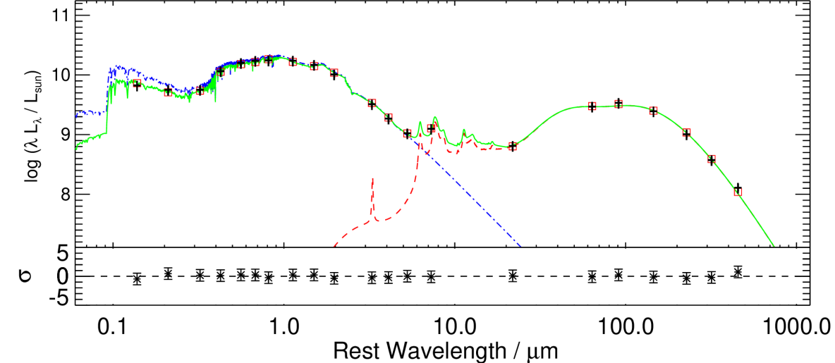
Figure 1: An example best-fit UV-mm SED (green solid line). Also overlaid are the best-fit unattenuated stellar SED (dot-dashed blue line) and the best-fit dust SED component (red dashed line). The model photometry associated with the best-fit SED is shown as the red squares, while the synthetic photometry derived from the simulations is shown as the black error bars (assuming a signal-to-noise ratio of 5 in every band). The lower panel shows the residuals of the synthetic photometry about the best-fit SED for each photometric band; we do not add noise to the photometry, and the uncertainties are included solely for the purposes of enabling us to use magphys.

magphys (da Cunha et al., 2008, hereafter DC08) is a publicly available SED fitting code that assumes an energy balance criterion to model the stellar emission of a galaxy consistently with its dust emission. By assuming that the energy absorbed from the intrinsic starlight by a two-component dust model (from Charlot & Fall, 2000, with the two components corresponding to an ambient diffuse interstellar medium (ISM) and embedded stellar birth clouds) is re-radiated in the far-infrared, it is possible to use the model to not only produce realistic best-fit SEDs for a wide variety of galaxies with different properties (see e.g. Smith et al., 2012; Hayward & Smith, 2015, and references therein) but also to derive Bayesian probabilistic estimates of their physical parameters by marginalising over the stellar and dust libraries.

Here we use the default version of magphys, which models the emission from stars using the Chabrier (2003) initial stellar mass function along with a library of 50,000 SFHs and stellar spectra taken from the well-known (unpublished) ‘CB07’ version of the Bruzual & Charlot (2003) simple stellar population models. The SFHs in the magphys stellar library consist of two components, a baseline exponentially declining star formation rate, with bursts randomly superposed. Approximately half of the SFHs in the library have experienced a burst in the past 2 Gyr, a feature which is critical for reliably recovering stellar masses (Michałowski et al., 2014).

The dust emission model used in magphys is described in detail in DC08, but to summarise, each dust SED consists of multiple optically thin modified blackbody profiles with different normalisations, temperatures and emissivity indices (see e.g. Hildebrand, 1983; Hayward et al., 2012; Smith et al., 2013, for a detailed description of modified blackbodies, and an analysis of using them to model dust emission in galaxies) describing dust grains of different sizes, along with a recipe for including emission from polycyclic aromatic hydrocarbons (PAHs). The primary adjustable components of the magphys far-IR model are a warm ‘birth-cloud’ dust component with emissivity index $\beta_{BC}=1.5$ and temperature between $30\leq T_{W}^{BC}\leq 60$ K, and a cool ‘diffuse ISM’ component with $\beta_{ISM}=2.0$ and $15\leq T_{C}^{ISM}\leq 25$ K, corresponding to the Charlot & Fall (2000) dust obscuration model applied to the stellar libraries.

magphys combines those stellar and dust-emission libraries to yield full UV to millimetre (mm) SEDs, which are then compared with the observed photometry by convolving the panchromatic models with a set of user-defined filter curves. It then uses the $\chi^{2}$ estimator to determine the goodness-of-fit for every combination of stellar and dust components that satisfies the energy balance criterion.

In this analysis, we use magphys to fit model SEDs to 21 different photometric bands, arbitrarily chosen to include data from GALEX at FUV and NUV wavelengths (e.g. Martin et al., 2005), the SDSS $ugriz$ bands (York et al., 2000), UKIDSS $JHK$ (Hewett et al., 2006), Spitzer Space Telescope IRAC 3.4 4.5, 5.8 and 8.0 $\mu$m, MIPS 24 and 70 $\mu$m (e.g. Werner et al., 2004), and Herschel Space Observatory data (Pilbratt et al., 2010) at 100, 160, 250, 350 and 500 $\mu$m. As for our previous work in Hayward & Smith (2015), our goal is to test magphys under idealised conditions and investigate systematics rather than effects arising from imperfect observational data (e.g. the difficulties of cross-identifying Herschel galaxies; Smith et al., 2011); we therefore do not add any noise to the input photometry. For the purposes of using magphys for the fitting however, we arbitrarily assume uncertainties of 20 per cent in every photometric band. Fig. 1 shows an example best-fit SED output by magphys; the synthetic photometry is shown as the black crosses with error bars while the best-fitting model photometry is shown by the red squares overlaid on the best-fit emergent SED (in green). The emergent SED is further decomposed into the best-fit intrinsic stellar model (blue, dot-dashedd line) and the best-fit IR template (red dashed line). The lower panel shows the residuals between the observed photometry and the best-fit model in each band in $\sigma$ units.

2.2 Recovering the SFHs and internal validation

In order to extract constraints on galaxy star formation histories from the public version of magphys we make several modifications to the code. We first calculate the sum of the relative probabilities, $P^{\prime}\equiv\exp(-\chi^{2}/2)$, and the weighted-mean stellar mass for each SFH in the magphys library, where the averaging is over every combination of starlight and dust SEDs that satisfies the energy balance criterion. We then marginalise these 50,000 relative probabilities over the library of SFHs. This method is analogous to the way magphys calculates probability distributions for parameters of interest (e.g. stellar mass), however unlike in the standard magphys implementation, we retain these data for every galaxy being studied for the purposes of determining the SFHs in post-processing.

Since the SFHs in the default magphys library vary in length (due to the different ages of the continuous component), and since they have different time resolutions, we linearly interpolate each SFH onto a common time grid, equally spaced in $\log$ look-back time at intervals of $\Delta\log T=0.05$.

Given the marginalised probabilities and the SFHs brought onto a consistent time resolution, we are able to determine median-likelihood SFHs by determining the 50^th percentile of the cumulative distribution of SFR as a function of look-back time. We also derive uncertainties on the median-likelihood SFH by determining the 16^th and 84^th percentiles of the distribution; these values are equivalent to the $\pm 1\sigma$ values in the limit of Gaussian-distributed uncertainties.

An example showing the information that we can derive is shown in Fig. 2, with the logarithm of the SFR on the ordinate and look-back time in Gyr on the abscissa. In this figure, we internally validate our method by feeding magphys synthetic photometry derived from one of the SEDs in the default library placed at $z=0.1$. We assume that each photometric datum has an associated uncertainty of 20 per cent. The best-fit SFH (which in this case corresponds to the true SFH by design, with photometric $\chi^{2}=0.0$) is shown in as the red line, and we also overlay the median-likelihood SFH (thick black line) along with the area enclosed by the $\pm 1\sigma$ uncertainties (grey shaded region). The median-likelihood SFH is inevitably a worse estimate of the true SFH than the best fit SFH in this case, given that the exact SFH of this galaxy is in the library; however, the true SFH is always within 1$\sigma$ of the median-likelihood values (including during the strong burst of star formation around 1 Gyr ago). We attribute the fact that the SFH uncertainties are not centred around the best-fit/true SFH to the prior distribution of SFHs in the magphys library (we will return to the topic of the SFH priors in what follows, however we note that the median-likelihood SFHs we recover here and elsewhere are considerably different from the median SFH of the magphys library, indicating that useful SFH constraints are being obtained from the photometry). We also calculate the total SFH probability (i.e. the sum of the probability in all SFHs defined at any given look-back time) as a function of look-back time; this is overlaid as the light-blue dot-dashed line in Fig. 2, with values indicated by the right-hand axis.

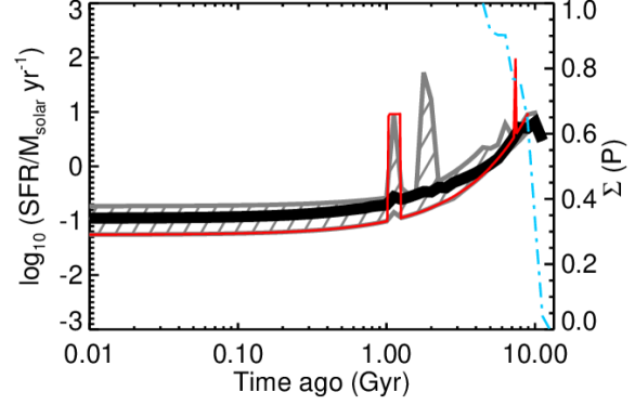
Figure 2: Recovering the SFR as a function of look-back time based on SED fitting of synthetic photometry for a model $z=0.1$ galaxy taken from the default magphys libraries, with assumed 20 per cent photometric uncertainties in every band. The best-fit SFH (which also corresponds to the true SFH in this case) is shown as the red line, while the median-likelihood SFH is overlaid as the thick black line, with the region bounded by the $\pm 1\sigma$ uncertainties shaded in grey. The dot-dashed light blue line shows the cumulative probability distribution of the SFH as a function of look-back time, derived by marginalising over the magphys SFH library, relative to the right-hand axis.

To quantify how well we are able to recover the SFHs of individual simulated galaxies, we define two parameters, $\chi^{2}_{\rm SFH}$ and $\Delta M/M$, as follows:

$$\chi^{2}_{\rm{SFH}}=\frac{1}{N}\sum_{t}\frac{\left({\rm SFR}_{{\rm model}}(t)-{\rm SFR}_{{\rm true}}(t)\right)^{2}}{\sigma_{\rm SFR}(t)^{2}},$$ (1)

and,

$$\frac{\Delta M}{M}=\frac{\sum_{t}|{\rm SFR}_{\rm model}(t)-{\rm SFR}_{\rm true}(t)|}{\sum_{t}{\rm SFR}_{\rm true}(t)},$$ (2)

where ${\rm SFR}_{\rm model}(t)$ represents either the SFH associated with the best-fitting SED template or the median-likelihood SFH, ${\rm SFR}_{\rm true}(t)$ is the known SFH of the simulation, $\sigma_{\rm SFR}(t)$ is the uncertainty on the median-likelihood SFH as a function of look-back time, and the summations are over the N bins in look-back time for which both the true SFH and the SFH being compared with are defined. $\chi^{2}_{\rm SFH}$ is thus a measure of how well any given SFH (e.g. the best-fit or median-likelihood that we recover) tallies with the true SFH that we know from the simulations (after accounting for the uncertainties), though we emphasize that we do not use use this parameter in any SED fitting. $\Delta M/M$ quantifies the integrated absolute difference between the model and known SFH as a fraction of the total mass of formed stars. Note that because the absolute difference is used, $\Delta M/M$ can be large even if the stellar mass is accurately recovered (because for the mass, time periods in which the true SFR is overestimated can be compensated for by time periods in which it is underestimated). In what follows, we will use these two parameters to inform our discussion of the results of using magphys to estimate the SFHs of simulated galaxies.

2.3 Simulations used for validation

To validate the method, we apply it to mock SEDs generated from hydrodynamical simulations of isolated disc galaxies and binary galaxy mergers (see Hayward & Smith 2015 for a detailed discussion of the merits of this type of external validation). Because the SFHs of the simulated galaxies are known, this approach enables us to test how well our method can successfully recover the true SFH from photometry alone. We do not add noise to the mock photometry; consequently, we test whether physical limitations prevent us from recovering the SFH even when we have perfect (i.e. noiseless) data.

We utilise a subset of the mock SEDs from the suite of simulations first presented in Lanz et al. (2014). The full dataset contains SEDs for four isolated disc galaxy simulations with stellar masses that range from $6\times 10^{8}$ to $4\times 10^{10}~{}\mathrm{M_{\odot}}$ and binary mergers of all possible combinations of progenitors (i.e. 10 mergers) for a single generic orbit. The merger mass ratios range from 1:1 to 1:69. The progenitor galaxies were designed to have properties (e.g. gas fractions) that are typical of galaxies in the local Universe; see Cox et al. (2008) for details. The progenitor discs are referred to as M0, M1, M2, and M3, in order of increasing stellar mass. The mergers are referred to using the labels of the two progenitors followed by an ‘e’ (because the ‘e’ orbit of Cox et al. 2008 was used), e.g. M3M2e. In this work, we present results from the isolated disc simulations (M0, M1, M2, and M3) and the M3M2e merger simulation.

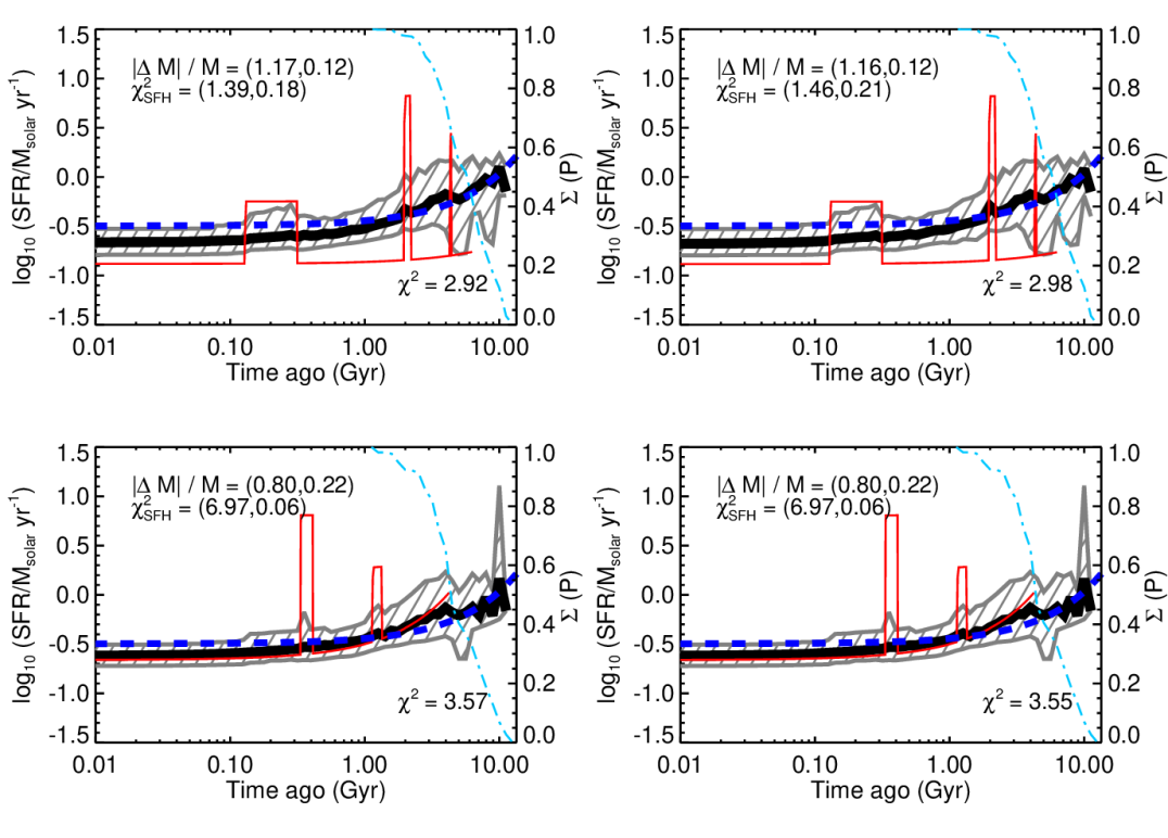
Figure 3: Constraints on the SFH of the first snapshot of the M2 simulation, where each panel shows the results for one of the individual viewing angles, modelled using magphys. The true SFH is shown by the dashed blue line, the best-fit estimate produced by magphys is shown as the red solid line, and the median-likelihood SFH is shown as the thick black line. The region enclosing the 16^th and 84^th percentiles of the SFH PDF at each look-back time is shown by the grey shaded region. The legend in the upper left of each panel details the values of $\Delta M/M$ and $\chi^{2}_{\rm SFH}$ for the best-fit and median-likelihood SFHs, respectively, while the lower-right legend shows the best-fit value of $\chi^{2}$ for each model. The light-blue dot-dashed line shows the SFH cumulative frequency distribution derived by marginalising over the magphys SFH library, relative to the right-hand axis. While the SFH of the model with the best fit to the photometry shows variation with viewing angle and spurious bursts not present in the true SFH, the median-likelihood SFH estimate is better-behaved.

We will now briefly summarise the details of the hydrodynamical simulations and mock SED generation, but we refer the reader to Lanz et al. (2014), Hayward & Smith (2015) and references therein for full details. First, idealised galaxies composed of a dark matter halo, gaseous and stellar discs, stellar bulge, and supermassive black hole were created following the procedure of Springel et al. (2005). Then, the dynamical evolution of each of the isolated discs and mergers was simulated using a modified version of the $N$-body/smoothed-particle hydrodynamics (SPH) code gadget-2 (Springel, 2005). The simulations directly include the effects of gravity, hydrodynamics, and radiative heating and cooling. The SFRs associated with individual gas particles are calculated according to a volume-density-dependent Kennicutt–Schmidt relation (Schmidt, 1959; Kennicutt, 1998) with a low-density threshold. Star particles are stochastically spawned from gas particles, where the probability that a given gas particle spawns a star particle is proportional to its SFR. Supernova feedback is modeled using the two-phase interstellar medium model of Springel & Hernquist (2003). Metal enrichment is treated by evolving each gas particle as a closed box. Black hole accretion and active galactic nucleus (AGN) feedback are included as described in Springel et al. (2005).

At various times throughout the simulations (every 10 or 100 Myr; times at which the SFR varies rapidly were sampled more frequently), ‘snapshots’ of the physical state of the simulation were saved. Then, in post-processing, three-dimensional (3D) dust radiative transfer was performed using the Monte Carlo radiative transfer code sunrise (Jonsson, 2006; Jonsson et al., 2010). This process proceeds as follows. First, the sources of radiation are specified: the star particles are assigned Starburst99 (Leitherer et al., 1999) single-age stellar population SEDs according to their ages and metallicities. The progenitor galaxies include stellar discs and bulges, and these star particles must be assigned ages and metallicities. The stellar disc is assumed to have formed with an exponentially declining SFH, whereas the bulge is assumed to have formed via an instantaneous burst. The metallicities of the stars that exist at the start of the simulations and the initial gas metallicity are specified via a profile that decreases exponentially with distance from the galaxy center. Both the SFHs for the stellar disc and bulge and the metallicity gradients have been constrained by comparisons with observations of local galaxies; see Rocha et al. (2008) for details. The star particles formed in the simulations have ages and metallicities that are determined self-consistently. We note that the resulting SEDs are rather insensitive to the assumed SFH for the stellar disc and bulge and metallicity gradient, especially after the first few hundred Myr (e.g. Hayward et al., 2011). The AGN particles are assigned luminosity-dependent template SEDs from Hopkins et al. (2007), which are based on observations of unreddened quasars. Subsequently, the dust distribution is calculated by projecting the metal content of the gas particles onto a 3D octree grid, assuming a dust-to-metals ratio of 0.4 (Dwek, 1998; James et al., 2002).

With the source positions, source SEDs and dust distribution in hand, radiative transfer is performed to calculate the effects of dust absorption and scattering. The thermal-equilibrium temperatures of dust grains, which depend on the local radiation field and the wavelength-dependent grain opacity, are calculated. Subsequently, radiation transfer of the resulting IR emission is performed. To account for dust self-absorption, the dust temperature calculation and IR radiation transfer are iterated until the temperatures converge. The calculation results in spatially resolved UV–mm SEDs of the galaxies viewed from multiple viewing angles (seven in our case). We sum the SEDs of all individual pixels to obtained galaxy-integrated SEDs and then convolve these with the appropriate filter response curves to obtain broadband photometry.

3 Results

In this section we will determine how well magphys can recover SFHs for two classes of simulations in which the answer is known, isolated disks and galaxy mergers. Both classes are of important diagnostic value: the isolated disk SFHs should be reasonably well-described by the simple exponentially-decaying or “$\tau$ model” SFH parametrisations in magphys, whilst we expect that the galaxy mergers have more complex and “bursty” SFHs (and as discussed in Section 2.1, bursts are randomly superposed on the magphys SFHs).

3.1 Isolated disc SFHs

Fig. 3 compares the best-fit and median-likelihood SFHs for four of the seven viewing angles from the first snapshot of the M2 simulation. In each panel, the true SFH (which is independent of viewing angle, of course) is shown as the dashed blue line; because this is the first snapshot, the SFH is that assumed for the stars that exist at the start of the simulation i.e. an exponentially declining SFH for the disc stars and an instantaneous burst for the bulge (see Section 2.3 for details). The best-fit SFH derived using magphys is shown by the red line, and the median-likelihood SFH is shown as the thick black line, with associated uncertainties indicated by the grey shaded region. The $\Delta M/M$ and $\chi^{2}_{\rm SFH}$ values for each viewing angle are shown in the upper-left legend in each panel, while the lower-right legends show the best-fit $\chi^{2}$. The dot-dashed light blue line in each panel shows the SFH cumulative frequency distribution of the model galaxy (relative to the right-hand axis), which is derived by marginalising over the magphys library of SFHs for each viewing angle.

It is immediately apparent from Fig. 3 that the best-fit SFH (red line) can vary depending on the viewing angle, while the median-likelihood SFH (thick black line) derived by marginalising over the SFHs in the default magphys library is rather more consistent. Furthermore, the best-fit SFH often falls outside the grey shaded region (which represents the range of $\pm 1\sigma$ on the SFH at each snapshot); in 3/7 cases it is systematically offset, while in a further 3 cases the best-fit SFH indicates the presence of starbursts which are not present in the true SFH. In stark contrast, the median-likelihood SFH is in good agreement with the true SFH at all values, once the uncertainties are taken into account. This is true even at large look-back times, where the median-likelihood SFH estimates and the associated uncertainties become angular and noisy; we attribute this effect partly to the difficulty of distinguishing between stellar populations older than $\sim 1$ Gyr, and partially due to the small number of SFHs in the magphys library that give acceptable fits to the synthetic photometry with sufficiently large ages. This effect is underlined by the plunge in the SFH cumulative probability distribution (dot-dashed light-blue lines) in each panel of Fig. 3. The $\Delta M/M$ values (representing the fractional mass discrepancy) are lower for the median-likelihood SFHs in each case; the best-fit SFHs containing bursts are also strongly disfavoured by the $\chi^{2}_{\rm SFH}$ values.

To ease comparison, and show all seven viewing angles, we overlay the individual best-fit and median-likelihood SFHs for each angle of the first snapshot in the M2 simulation with one another in Fig. 4. It is immediately apparent that the best-fit SFHs (in red) are much less consistent between angles and show worse agreement with the true SFH (dashed blue line) than the median-likelihood SFHs (thick black lines). To test whether this behaviour is due to the choice of prior, we re-run our internal validation discussed in section 2.2, excluding the true SFH from the model library. We find that under these conditions our internal validation returns a similar disagreement between the best-fit and true SFHs, suggesting that the best-fit SFH is unreliable even with a realistic prior on the SFHs. We speculate that this behaviour may be due to parameter degeneracies even in panchromatic broad-band galaxy SEDs.

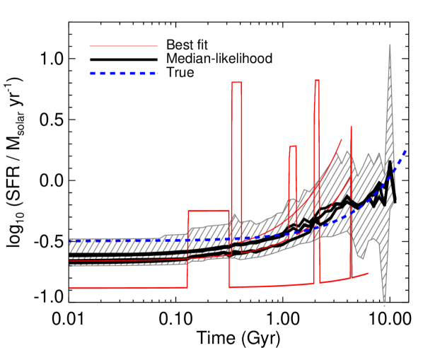
Figure 4: SFHs recovered for the seven different viewing angles to the first snapshot of the M2 isolated disk simulation shown in Fig. 3. The true SFH is shown as the blue dashed line, while the best-fitting SFHs for each of the seven viewing angles are shown as the red lines. The median-likelihood SFHs for each viewing angle are shown as the thick black lines, while the shaded grey region shows the average uncertainty associated with the median-likelihood SFHs. The contrast between the SFH of the best-fit model and the median-likelihood SFH (in terms of both reliability and fidelity) is clear.

In Fig. 5 we compare four of the SFHs constructed using the modified magphys with the true SFH for the last snapshot of the simulation. This presents a useful test: because stars (more precisely, star particles that are analogous to star clusters) have formed throughout the simulation according to the assumed volume-density-dependent Kennicutt-Schmidt relation (see Section 2.3 for details), these SFHs do not have a simple, generic analytic form, as can be seen in Fig. 5.

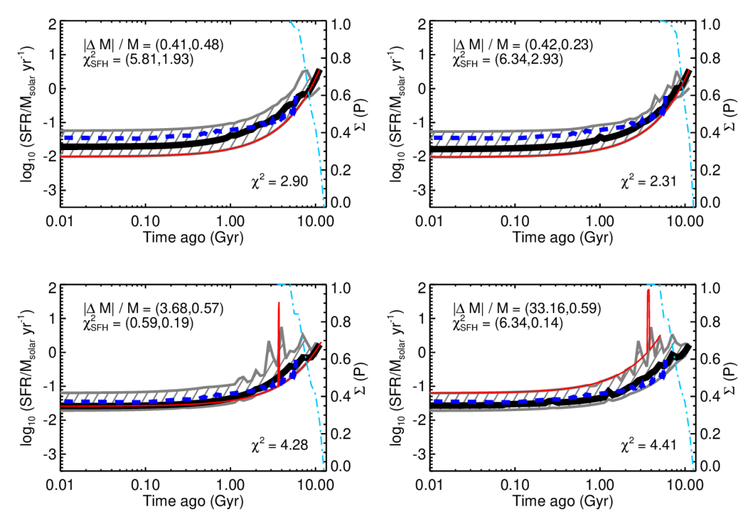
Figure 5: SFHs recovered for the final snapshot of the M2 simulation; the true SFH compiled from the individual simulation snapshots is shown by the dashed blue line, while the best-fit SFH from magphys  is overlaid with a red solid line. The thick black line represents the median-likelihood SFH, while the grey region shows the range of $\pm 1\sigma$ about the median-likelihood SFH as a function of look-back time. The legends are as in Fig. 3. The median-likelihood SFH is once again preferred over the SFH of the model that is the best-fit to the photometry.

Once more, the $\chi^{2}_{\rm SFH}$ and $\Delta M/M$ values point to greater fidelity in the median-likelihood SFHs rather than the best-fit values, which also show greater variation with viewing angle and the presence of bursts which do not exist in the true SFH. This variation is more apparent in Fig. 6, in which we directly overlay the best-fit and median-likelihood SFHs for each of the seven viewing angles. The colour scheme is as in Figs. 3, 4 & 5. The true SFH constructed from the individual snapshots of the M2 simulation is arguably a better test of magphys than the previous tests, since it should be more realistic for an evolving disk galaxy. That there is such good agreement between the median-likelihood SFH derived using magphys and the true SFH offers considerable encouragement for using magphys in this way.

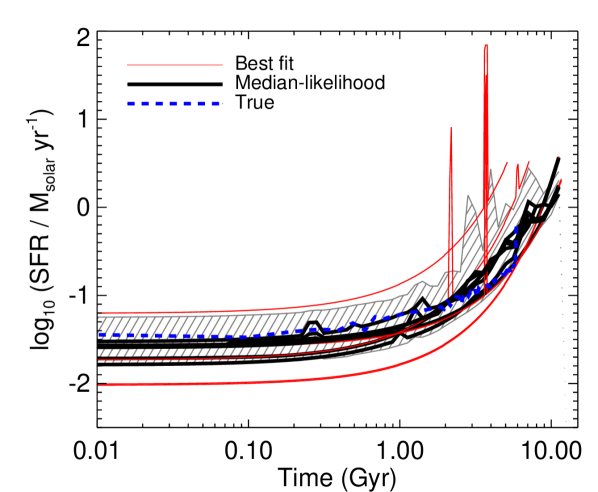
Figure 6: SFHs recovered for the seven different viewing angles to the last snapshot of the M2 isolated disk simulation shown in Fig. 5. The true SFH is shown as the dashed blue line, while the best-fitting SFHs for each viewing angle are shown by the red lines. The median-likelihood SFHs are shown as thick black lines, while the shaded grey region shows the average uncertainty associated with the median-likelihood SFHs. The median-likelihood SFH is more reliable and a better approximation of the true SFH than the SFH of the best-fit model.

3.2 Galaxy merger SFHs

We now turn our attention to the M3M2e simulation, corresponding to a major galaxy merger with a mass ratio of 2.3:1. We examine, in particular, two of the time snapshots after the individual components have coalesced, at which point magphys is able to produce an acceptable fit to the model photometry. These snapshots are of particular interest, since the true SFHs drawn from the simulations are dominated by a recent, extended, and merger-induced burst of star formation and are considerably more complicated than the simple “exponentially declining + burst” SFHs assumed in the version of magphys used here. As a result, they present an excellent test of how well magphys can perform under this particularly challenging scenario using the standard libraries.

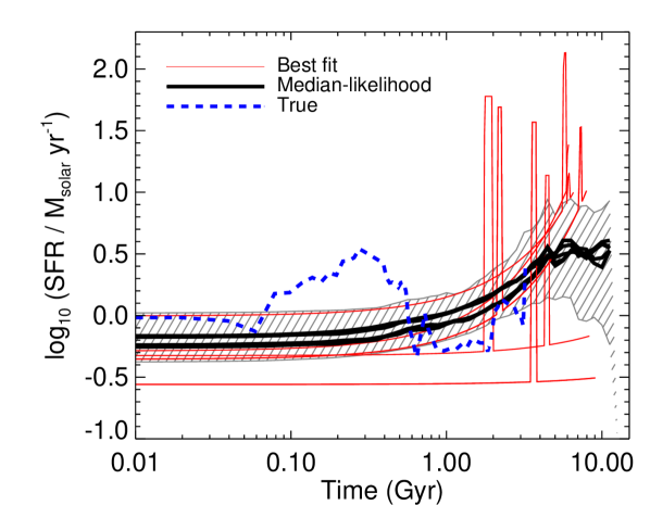
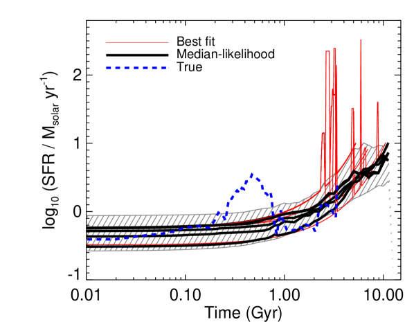
Figure 7: SFHs recovered for the seven different viewing angles for two snapshots taken from the M3M2e merger simulation. The true SFH is again shown as the dashed blue line, while the best-fitting SFH for each viewing angle is shown by the red lines. The median-likelihood SFHs are shown as thick black lines, while the shaded grey region shows the average uncertainty associated with the median-likelihood SFHs. The left plot shows the SFH recovered from the 60th snapshot, corresponding to $\sim 0.3$ Gyr after the time of the peak in the merger-induced starburst, while the right plot shows the SFH recovered for the 70th snapshot, $\sim 0.5$ Gyr after the peak SFR. Neither the best-fit or median-likelihood SFH is able to recover the main burst of merger-induced star formation.

Fig. 7 presents the results for snapshots taken around 0.3 and 0.5 Gyr after the peak of the merger-induced starburst in the left- and right-hand panels, respectively. The starburst can be clearly seen in the true SFHs (blue dashed lines), though the SFHs reconstructed from magphys (whether they are best-fit or median-likelihood) are clearly incorrect, despite the $\chi^{2}$ values indicating a good fit to the photometry in both cases (and despite Hayward & Smith, 2015, having demonstrated that it is still possible to derive reasonable e.g. SFRs and stellar masses under similar conditions). Once more the magphys library SFHs associated with the best-fit to the photometry are littered with spurious bursts of star formation, thus highlighting the difficulty in interpreting burst-related properties. We shall return to these points in Section 4.

4 Discussion

4.1 Median-likelihood vs. best-fitting SFHs

In Section 3, we noted that the median-likelihood SFH estimates are more consistent with viewing angle and agree better with the true SFH than the best-fit SFH that we derive. Above, we showed a few examples to demonstrate our method and highlight the merits of the median-likelihood SFHs. To assuage any concerns that we have only shown the best examples and present a more complete analysis, we now compare the two possibilities quantitatively by using equations 1 and 2 to calculate $\chi^{2}_{\rm SFH}$ and $\Delta M/M$ for each of the seven viewing angles to the first and last snapshots of the isolated disk simulations, for which magphys recovers a good fit. We have not included the merger simulations because the SFHs are generally not well recovered owing to the merger SFHs differing drastically from those assumed in the standard magphys library. $\chi^{2}_{\rm SFH}$ and $\Delta M/M$ tell us how well the SFH is recovered by our modified version of magphys, though we emphasize again that these parameters are not included in the SED fitting itself (since it can be rather difficult to know the true SFH for a real galaxy a priori).

The left-hand panel of Fig. 8 shows a comparison of the values of $\chi^{2}_{\rm SFH}$ returned for the best-fit (“BF”, shown on the $x$-axis) and median-likelihood (“M-L”, on the $y$-axis) SFHs derived by our modified version of magphys. The fact that the vast majority of the data points lie below the dotted line (indicative of parity) highlights that our analysis strongly favours the median-likelihood SFHs over the individual SFH that provides the best fit to the photometry. The right-hand panel shows the same preference for the median-likelihood SFHs in terms of $\Delta M/M$, indicating the best-fit SFHs show a larger absolute stellar mass discrepancy than the median-likelihood SFHs (this is expected given their poorer $\chi^{2}_{\rm SFH}$). We note that it is possible to have a large $\Delta M/M$ and still recover a reasonable stellar mass estimate, since $\Delta M/M$ is extremely punitive. This is because $\Delta M/M$ accounts for the time at which the stars are formed, whereas the stellar mass can be recovered accurately if times at which the SFR is overestimated are compensated for by times at which it is underestimated. $\log_{10}($$\Delta M/M$$)=0.0$ implies an absolute integrated mass discrepancy between the true and model SFH that is equal to the present-day stellar mass. In Smith et al. (2013) we noted a slight preference for median-likelihood parameter estimates (e.g. dust luminosity, or isothermal dust temperature) due to their slightly lower bias relative to the best fit parameters; here the preference for the median likelihood SFHs is rather stronger.

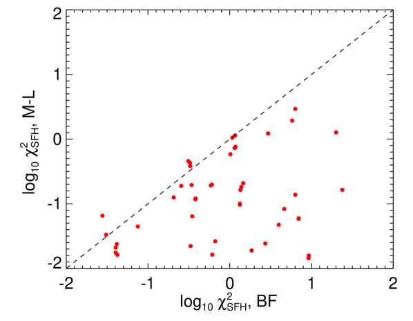
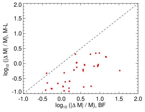
Figure 8: Comparison between the values of $\chi^{2}_{\rm SFH}$ (left panel) and $\Delta M/M$ (right panel) for the first and last snapshots of the isolated disk simulations, calculated for the median-likelihood (“M-L”, on the $y$-axis) and best-fit (“BF”, on the $x$-axis) SFHs derived using our modified version of magphys. The dashed line indicates parity, i.e. no preference for either type of SFH. In the right-hand panel $\log_{10}($$\Delta M/M$$)=0.0$ implies an absolute integrated mass discrepancy between the true and model SFH that is equal to the present-day stellar mass. Both the $\chi^{2}_{\rm SFH}$ and $\Delta M/M$ comparisons indicate that the median-likelihood SFHs tend to better represent the true SFHs.

Perhaps the most obviously unsatisfactory features of the best-fit SFHs are the inconsistency with viewing angle and the unreliable behaviour of the bursts. In the former case, the inconsistency with viewing angle of the best-fit SFHs is of particular concern for real observations, where the line-of-sight to any extragalactic object is fixed. Regarding the latter issue, the best-fit SFHs often include spurious bursts for the isolated disk simulations (where they should not be present). For the the merger simulations (where they should be present), bursts appear at the wrong point in the SFH. The median-likelihood SFHs can mitigate the viewing angle dependence and show no evidence for spurious bursts of star formation for the isolated disk simulations. However, they are also unable to approximate the complex SFHs of the merger simulations, likely because the simple analytic form for the SFHs contained in the standard magphys library is too restrictive (it contains bursts with a constant, elevated SFR that last between 30 and 300 Myr; da Cunha et al., 2008); we will discuss this issue in detail below.

That the best-fit SFHs appear so unreliable in comparison to the median-likelihood values is perhaps not surprising: if the true SFHs are not present in the magphys prior, then it is only by marginalising over the SFH library that we could hope to recover something approaching the truth. This is also the case in the real Universe: we cannot reasonably expect synthetic libraries to contain every possible galaxy SFH (even if they did have an analytic form). This provides further motivation for adopting our statistical approach to deriving realistic galaxy SFHs from photometry.

4.2 The need for more complex SFHs

That our method was unable to recover SFHs of the major mergers is perhaps not surprising, given the complex form of the merger simulations’ SFHs. We are unable to approximate such SFHs even by marginalising over the entire magphys library, though the merger simulation SFHs are by no means the most complex or extreme that exist in the real Universe (or even the latest simulations e.g. Hopkins et al., 2014). We suggest that it would be extremely desirable to include more complex SFHs in the magphys libraries if we wish to use it to study the individual star formation histories of galaxies in detail based on photometry alone. Though they represent a succinct and physically-motivated means of describing rudimentary composite stellar populations, the shortcomings of the so-called “$\tau$ models” are clear (see e.g. Lee et al., 2009, 2010; Conroy, 2013; Simha et al., 2014) and recent studies have noted a preference for delayed $\tau$ models (consisting of a linear rise preceding the exponentially declining SFR; e.g. Pforr et al., 2012; da Cunha et al., 2015), though they are still analytic. Whatever the form of the continuous underlying SFH, it will remain desirable to have a more physical (e.g. Gaussian or log-normal distributed) description of the bursts of star formation, rather than the top-hat models currently implemented.

One promising approach is that adopted by Pacifici et al. (2012), who built half a million non-parametric SFHs by performing a semi-analytic post-treatment of the Millenium simulation (Springel et al., 2005). The downside of the increased complexity that we advocate is the increased computation necessary for what is already a relatively load-intensive task. The desire for a more varied set of SFHs can surely only increase as we embark upon the survey era heralded by first light of e.g. the Large Synoptic Survey Telescope (Ivezic et al., 2008) and the Square Kilometre Array, although the consistent modelling and interpretation of these disparate data sets requires considerable further investigation if we are to truly exploit their immense potential (e.g. Smith et al., 2014).

4.3 The utility of the mock SED-based validation

Having presented the results of our validation based on fitting the SEDs of simulated galaxies, it is worthwhile to consider what this controlled experiment tested. Because the simulations represent each galaxy’s stellar population as the sum of $\sim 10^{5}$ discrete particles, the resulting SEDs reflect a diversity of ages and metallicities, similar to real galaxies. Effects that make recovering SFHs from SED modelling challenging include the fact that young stars tend to dominate the luminosity at UV–optical wavelengths, thereby obscuring older stellar populations (see e.g. Sorba & Sawicki, 2015, for a recent discussion); stellar isochrones change little at late times, which makes it difficult to infer the shape of the early SFH (e.g. Bruzual & Charlot, 2003); the true SFH can differ significantly from the assumed parametric form (as discussed above); dust reddening is degenerate with stellar age (e.g. Gordon et al., 1997); and differential obscuration can cause stars of different ages to be attenuated by different amounts (e.g. Charlot & Fall, 2000). All of these potential barriers to SFH recovery are included in the simulations. It is thus very encouraging that our method was able to recover the SFHs of the simulated isolated disk galaxies relatively well, at least using the median-likelihood SFHs.

5 Conclusions

We have presented modifications to the public version of the magphys SED-fitting code (da Cunha et al., 2008) which enable statistical estimates of the star formation histories of individual galaxies using photometric information alone (assuming that the redshift is precisely known). Though magphys is not intended for this purpose, our approach – which uses the standard magphys stellar and dust SED libraries – has been validated both internally (by “feeding” the code synthetic photometry corresponding to an arbitrarily chosen SFH in the magphys library) and externally. Our external validation made extensive use of state-of-the-art simulated ultraviolet to millimetre wavelength photometry derived by performing three-dimensional dust radiative transfer on SPH simulations from Lanz et al. (2014) using the sunrise code (Jonsson, 2006; Jonsson et al., 2010). This approach to validating SED fitting codes, which is discussed in detail in Hayward & Smith (2015, in which we highlighted how well magphys can recover various properties of simulated galaxies, including the SFR, stellar mass and dust mass), gives us several advantages over real observations, and enables us to test the efficacy of magphys for recovering SFHs under idealised conditions. Our main findings can be summarised as follows:

• Using our modified version of magphys, we are able to reliably recover the SFHs of isolated disk galaxies, provided that we marginalise over the library of SFHs. Marginalising over the libraries enables us to calculate median-likelihood SFHs in a manner analogous to how magphys calculates galaxy parameters (e.g. stellar mass, dust luminosity) and naturally yields SFH uncertainties by estimating the percentiles of the SFH probability distribution functions as a function of look-back time.

• We find that SFHs corresponding to the best-fit of the magphys model SEDs to the synthetic photometry are unreliable. This is manifest by large variations with viewing angle to the galaxy (the simulations include seven different viewing angles towards each model galaxy snapshot) and spurious bursty SFHs for galaxies which in truth have smoothly varying SFHs. The SFHs corresponding to the best photometric fit are a considerably worse estimate of the true SFH – which is known for the simulations – than the median-likelihood SFH. We parametrise our SFH fidelity by introducing $\chi^{2}_{\rm SFH}$ (a goodness-of-fit comparing derived SFH estimates with the true values known from the simulation) and $\Delta M/M$ (an estimate of the absolute mass differential between the true and modelled SFHs), which consistently favour the median-likelihood SFHs. We emphasise that neither of these parameters is used in the SED fitting itself, which is based purely on fitting model libraries to the synthetic photometry.

• We are unable to recover more complex SFHs, for example in the aftermath of a major merger-induced starburst, despite deriving a statistically acceptable fit to the photometric data (i.e. a reasonable $\chi^{2}$ goodness-of-fit parameter). This is particularly noteworthy given that in Hayward & Smith (2015), we were able to reliably determine properties (such as stellar mass, star formation rate, specific star formation rate and dust luminosity) of a post-merger galaxy in this regime. It may be possible to better recover such complex SFHs by using SED templates based on SFHs extracted from semi-analytical models or cosmological simulations.

• The best-fit SFHs often contain spurious bursts, and even when there are bursts in the true SFHs, their properties (e.g. time of occurrence and duration) are not well recovered. Thus, one should interpret the relevant outputs, such as the stellar mass formed in bursts, with extreme caution.

To summarize, we recommend that the utmost care be exercised in the interpretation of SFHs estimated from photometric data, and suggest that it is essential to marginalise over a range of different possible SFHs if any scientific value is required from their analysis (either studying individual galaxies, or for example studying the contribution of different galaxy samples to the evolving cosmic star formation rate density). This caution should be further heightened if there is reason to suspect a complex SFH (e.g. morphological tidal features, large far-infrared luminosity, etc) unless an appropriate wide range of possibilities is explicitly taken into account.

References

- Agertz et al. (2007) Agertz O. et al., 2007, MNRAS, 380, 963
- Bauer & Springel (2012) Bauer A., Springel V., 2012, MNRAS, 423, 2558
- Behroozi et al. (2010) Behroozi P. S., Conroy C., Wechsler R. H., 2010, ApJ, 717, 379
- Bernard et al. (2015) Bernard E. J. et al., 2015, MNRAS, 446, 2789
- Bertelli et al. (1992) Bertelli G., Mateo M., Chiosi C., Bressan A., 1992, ApJ, 388, 400
- Bruzual & Charlot (2003) Bruzual G., Charlot S., 2003, MNRAS, 344, 1000
- Chabrier (2003) Chabrier G., 2003, PASP, 115, 763
- Charlot & Fall (2000) Charlot S., Fall S. M., 2000, ApJ, 539, 718
- Cid Fernandes et al. (2005) Cid Fernandes R., Mateus A., Sodré L., Stasińska G., Gomes J. M., 2005, MNRAS, 358, 363
- Cignoni & Tosi (2010) Cignoni M., Tosi M., 2010, Advances in Astronomy, 2010, 3
- Cohn & van de Voort (2015) Cohn J. D., van de Voort F., 2015, MNRAS, 446, 3253
- Conroy (2013) Conroy C., 2013, ARA&A, 51, 393
- Cox et al. (2008) Cox T. J., Jonsson P., Somerville R. S., Primack J. R., Dekel A., 2008, MNRAS, 384, 386
- da Cunha et al. (2008) da Cunha E., Charlot S., Elbaz D., 2008, MNRAS, 388, 1595
- da Cunha et al. (2015) da Cunha E. et al., 2015, ApJ, 806, 110
- Dolphin (2002) Dolphin A. E., 2002, MNRAS, 332, 91
- Dolphin (2013) Dolphin A. E., 2013, ApJ, 775, 76
- Dwek (1998) Dwek E., 1998, ApJ, 501, 643
- Gennaro et al. (2015) Gennaro M., Tchernyshyov K., Brown T., Gordon K., 2015, arXiv:1504.04865
- Gordon et al. (1997) Gordon K. D., Calzetti D., Witt A. N., 1997, ApJ, 487, 625
- Grocholski et al. (2012) Grocholski A. J., van der Marel R. P., Aloisi A., Annibali F., Greggio L., Tosi M., 2012, AJ, 143, 117
- Guo et al. (2010) Guo Q., White S., Li C., Boylan-Kolchin M., 2010, MNRAS, 404, 1111
- Harris & Zaritsky (2001) Harris J., Zaritsky D., 2001, ApJS, 136, 25
- Hayward et al. (2012) Hayward C. C., Jonsson P., Kereš D., Magnelli B., Hernquist L., Cox T. J., 2012, MNRAS, 424, 951
- Hayward et al. (2011) Hayward C. C., Kereš D., Jonsson P., Narayanan D., Cox T. J., Hernquist L., 2011, ApJ, 743, 159
- Hayward et al. (2014a) Hayward C. C. et al., 2014a, MNRAS, 445, 1598
- Hayward & Smith (2015) Hayward C. C., Smith D. J. B., 2015, MNRAS, 446, 1512
- Hayward et al. (2014b) Hayward C. C., Torrey P., Springel V., Hernquist L., Vogelsberger M., 2014b, MNRAS, 442, 1992
- Heavens et al. (2004) Heavens A., Panter B., Jimenez R., Dunlop J., 2004, Nat, 428, 625
- Heavens et al. (2000) Heavens A. F., Jimenez R., Lahav O., 2000, MNRAS, 317, 965
- Hernandez et al. (2000) Hernandez X., Gilmore G., Valls-Gabaud D., 2000, MNRAS, 317, 831
- Hernandez et al. (1999) Hernandez X., Valls-Gabaud D., Gilmore G., 1999, MNRAS, 304, 705
- Hewett et al. (2006) Hewett P. C., Warren S. J., Leggett S. K., Hodgkin S. T., 2006, MNRAS, 367, 454
- Hidalgo et al. (2011) Hidalgo S. L. et al., 2011, ApJ, 730, 14
- Hildebrand (1983) Hildebrand R. H., 1983, QJRAS, 24, 267
- Hopkins et al. (2014) Hopkins P. F., Kereš D., Oñorbe J., Faucher-Giguère C.-A., Quataert E., Murray N., Bullock J. S., 2014, MNRAS, 445, 581
- Hopkins et al. (2007) Hopkins P. F., Richards G. T., Hernquist L., 2007, ApJ, 654, 731
- Ivezic et al. (2008) Ivezic Z. et al., 2008, arXiv:0805.2366
- James et al. (2002) James A., Dunne L., Eales S., Edmunds M. G., 2002, MNRAS, 335, 753
- Johnson et al. (2013) Johnson B. D. et al., 2013, ApJ, 772, 8
- Jonsson (2006) Jonsson P., 2006, MNRAS, 372, 2
- Jonsson et al. (2010) Jonsson P., Groves B. A., Cox T. J., 2010, MNRAS, 403, 17
- Kauffmann et al. (2003a) Kauffmann G. et al., 2003a, MNRAS, 341, 33
- Kauffmann et al. (2003b) Kauffmann G. et al., 2003b, MNRAS, 341, 54
- Kennicutt (1998) Kennicutt R. C., 1998, ApJ, 498, 541
- Koleva et al. (2009) Koleva M., Prugniel P., Bouchard A., Wu Y., 2009, A&A, 501, 1269
- Lanz et al. (2014) Lanz L., Hayward C. C., Zezas A., Smith H. A., Ashby M. L. N., Brassington N., Fazio G. G., Hernquist L., 2014, ApJ, 785, 39
- Lee et al. (2010) Lee S.-K., Ferguson H. C., Somerville R. S., Wiklind T., Giavalisco M., 2010, ApJ, 725, 1644
- Lee et al. (2009) Lee S.-K., Idzi R., Ferguson H. C., Somerville R. S., Wiklind T., Giavalisco M., 2009, ApJS, 184, 100
- Leitherer et al. (1999) Leitherer C. et al., 1999, ApJS, 123, 3
- Lewis et al. (2015) Lewis A. R. et al., 2015, arXiv:1504.03338
- Martin et al. (2005) Martin D. C. et al., 2005, ApJL, 619, L1
- Mathis et al. (2006) Mathis H., Charlot S., Brinchmann J., 2006, MNRAS, 365, 385
- McQuinn et al. (2010) McQuinn K. B. W. et al., 2010, ApJ, 721, 297
- Michałowski et al. (2014) Michałowski M. J., Hayward C. C., Dunlop J. S., Bruce V. A., Cirasuolo M., Cullen F., Hernquist L., 2014, A&A, 571, A75
- Monachesi et al. (2012) Monachesi A., Trager S. C., Lauer T. R., Hidalgo S. L., Freedman W., Dressler A., Grillmair C., Mighell K. J., 2012, ApJ, 745, 97
- Mundy et al. (2015) Mundy C. J., Conselice C. J., Ownsworth J. R., 2015, MNRAS, 450, 3696
- Noll et al. (2009) Noll S., Burgarella D., Giovannoli E., Buat V., Marcillac D., Muñoz-Mateos J. C., 2009, A&A, 507, 1793
- Ocvirk et al. (2006) Ocvirk P., Pichon C., Lançon A., Thiébaut E., 2006, MNRAS, 365, 46
- Olsen (1999) Olsen K. A. G., 1999, AJ, 117, 2244
- Pacifici et al. (2012) Pacifici C., Charlot S., Blaizot J., Brinchmann J., 2012, MNRAS, 421, 2002
- Panter et al. (2003) Panter B., Heavens A. F., Jimenez R., 2003, MNRAS, 343, 1145
- Pereira-Santaella et al. (2015) Pereira-Santaella M. et al., 2015, arXiv:1502.07965
- Pforr et al. (2012) Pforr J., Maraston C., Tonini C., 2012, MNRAS, 422, 3285
- Pilbratt et al. (2010) Pilbratt G. L. et al., 2010, A&A, 518, L1
- Reichardt et al. (2001) Reichardt C., Jimenez R., Heavens A. F., 2001, MNRAS, 327, 849
- Rocha et al. (2008) Rocha M., Jonsson P., Primack J. R., Cox T. J., 2008, MNRAS, 383, 1281
- Sanna et al. (2009) Sanna N. et al., 2009, ApJL, 699, L84
- Schmidt (1959) Schmidt M., 1959, ApJ, 129, 243
- Shamshiri et al. (2015) Shamshiri S., Thomas P. A., Henriques B. M., Tojeiro R., Lemson G., Oliver S. J., Wilkins S., 2015, arXiv:1501.05649
- Simha et al. (2014) Simha V., Weinberg D. H., Conroy C., Dave R., Fardal M., Katz N., Oppenheimer B. D., 2014, arXiv:1404.0402
- Small et al. (2013) Small E. E., Bersier D., Salaris M., 2013, MNRAS, 428, 763
- Smethurst et al. (2015) Smethurst R. J. et al., 2015, MNRAS, 450, 435
- Smith et al. (2012) Smith D. J. B. et al., 2012, MNRAS, 427, 703
- Smith et al. (2011) Smith D. J. B. et al., 2011, MNRAS, 416, 857
- Smith et al. (2013) Smith D. J. B. et al., 2013, MNRAS, 436, 2435
- Smith et al. (2014) Smith D. J. B. et al., 2014, MNRAS, 445, 2232
- Snyder et al. (2013) Snyder G. F., Hayward C. C., Sajina A., Jonsson P., Cox T. J., Hernquist L., Hopkins P. F., Yan L., 2013, ApJ, 768, 168
- Sorba & Sawicki (2015) Sorba R., Sawicki M., 2015, arXiv:1506.01653
- Sparre et al. (2015) Sparre M. et al., 2015, MNRAS, 447, 3548
- Springel (2005) Springel V., 2005, MNRAS, 364, 1105
- Springel (2010) Springel V., 2010, MNRAS, 401, 791
- Springel et al. (2005) Springel V., Di Matteo T., Hernquist L., 2005, MNRAS, 361, 776
- Springel & Hernquist (2003) Springel V., Hernquist L., 2003, MNRAS, 339, 289
- Springel et al. (2005) Springel V. et al., 2005, Nat, 435, 629
- Tojeiro et al. (2007) Tojeiro R., Heavens A. F., Jimenez R., Panter B., 2007, MNRAS, 381, 1252
- Tojeiro et al. (2013) Tojeiro R. et al., 2013, MNRAS, 432, 359
- Tojeiro et al. (2009) Tojeiro R., Wilkins S., Heavens A. F., Panter B., Jimenez R., 2009, ApJS, 185, 1
- Tolstoy & Saha (1996) Tolstoy E., Saha A., 1996, ApJ, 462, 672
- Torrey et al. (2015) Torrey P. et al., 2015, MNRAS, 447, 2753
- Tosi et al. (1989) Tosi M., Greggio L., Focardi P., 1989, Ap&SS, 156, 295
- Tosi et al. (1991) Tosi M., Greggio L., Marconi G., Focardi P., 1991, AJ, 102, 951
- Walcher et al. (2011) Walcher J., Groves B., Budavári T., Dale D., 2011, Ap&SS, 331, 1
- Walmswell et al. (2013) Walmswell J. J., Eldridge J. J., Brewer B. J., Tout C. A., 2013, MNRAS, 435, 2171
- Weisz et al. (2011) Weisz D. R. et al., 2011, ApJ, 739, 5
- Weisz et al. (2013) Weisz D. R., Dolphin A. E., Skillman E. D., Holtzman J., Dalcanton J. J., Cole A. A., Neary K., 2013, MNRAS, 431, 364
- Weisz et al. (2014) Weisz D. R., Dolphin A. E., Skillman E. D., Holtzman J., Gilbert K. M., Dalcanton J. J., Williams B. F., 2014, ApJ, 789, 147
- Weisz et al. (2008) Weisz D. R., Skillman E. D., Cannon J. M., Dolphin A. E., Kennicutt, Jr. R. C., Lee J., Walter F., 2008, ApJ, 689, 160
- Werner et al. (2004) Werner M. W. et al., 2004, ApJS, 154, 1
- Williams et al. (2015) Williams B. F. et al., 2015, arXiv:1504.02120
- York et al. (2000) York D. G. et al., 2000, AJ, 120, 1579
- Yuk & Lee (2007) Yuk I.-S., Lee M. G., 2007, ApJ, 668, 876