Extending the applicability of Thermal Dynamics to Evolutionary Biology.

Abstract

In the past years, a remarkable mapping has been found between the dynamics of a population of $M$ individuals undergoing random mutations and selection, and that of a single system in contact with a thermal bath with temperature $1/M$. This correspondence holds under the somewhat restrictive condition that the population is dominated by a single type at almost all times, punctuated by rare successive mutations. Here we argue that such thermal dynamics will hold more generally, specifically in systems with rugged fitness landscapes. This includes cases with strong clonal interference, where a number of concurrent mutants dominate the population. The problem becomes closely analogous to the experimental situation of glasses subjected to controlled variations of parameters such as temperature, pressure or magnetic fields. Non-trivial suggestions from the field of glasses may be thus proposed for evolutionary systems – including a large part of the numerical simulation procedures – that in many cases would have been counter intuitive without this background.

I Introduction

The dynamics of a population of $M$ individuals reproducing and undergoing random mutations and selection has long been recognized to bear a resemblance with a system driven by a ‘fitness potential’, with an element of ‘noise’ given by random fluctuations that are the larger, the smaller the total population (see, e.g. crow_introduction_1970 ; peliti_introduction_1997 ). However, the stochastic dynamics of a system in contact with a thermal bath satisfy the relation of ‘detailed-balance’ – the condition that the bath is itself in thermal equilibrium – obviously not applicable in general to an evolutionary dynamics with mutation and selection. A known exception happens when the population is dominated by a single mutant at any time, whose identity changes in rare and rapid ‘sweeps’ in which a new mutant fixes tsimring_rna_1996 ; lynch_lower_2011 ; neher_emergence_2013 ; sella_application_2005 ; mustonen_fitness_2010 , see Fig. 1c noteone . It turns out that in that special case berg_stochastic_2003 ; berg_adaptive_2004 ; sella_application_2005 ; barton_application_2009 , the analogy becomes a strict mathematical correspondence, opening the door to statistical mechanical reasoning for evolving systems.

In spite of its potential, this remarkable and somewhat counter-intuitive mapping has attracted relatively modest attention among physicists, partly because of the restrictive conditions necessary for it to hold. The purpose of this paper is to show that the correspondence to thermal dynamics is in fact, given an appropriate interpretation of observations, more robust for rugged fitness landscapes, where the changes in fitness in each beneficial mutation are small. Importantly, the same temperature is associated with the thermal dynamics in all cases.

As we shall see, the basic idea is that an essential ingredient for the correspondence is a timescale-separation between the rate of reproduction and the rate of fitness improvement, a separation which arises naturally in the evolution on rugged landscapes (see e.g. elena_microbial_2003 ) We then argue that provided that a proper averaging of observables over short times is applied, one may extend the applicability of detailed-balance, including conditions where several different mutant lineages compete simultaneously for fixation (clonal interference), and the changes in fitness in a single mutation (selective advantage) are less restrictive than before.

This paper is organized as follows: in section II we review the emergence of thermal dynamics, using the ‘House of Cards’ model as an example. We also discuss there the limitations of the development. In section III we very briefly review an extremely general, and in this context very important fact: a system that is optimizing slowly will necessarily exhibit fast and slow degrees of freedom, the timescale-separation between these increases as the system evolves, and, concomitantly, the actual number of slow degrees of freedom diminishes. In section IV we shall discuss how, if one concentrates on the slow degrees of freedom, the detailed balance property has a wider domain of validity. In section V we test this with a non-trivial model: constraint optimization of XorSAT problems with Boolean variables (we have also tried SAT, with similar results). The purpose here is not to argue in favor of the biological relevance of such models, but just to test our developments in a highly non-trivial case. The last part of the paper, section VI, is dedicated to suggested applications of this correspondence.

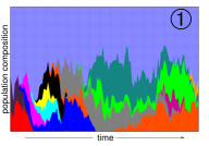
(a)

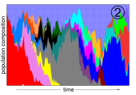
(b)

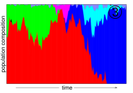
(c)

Figure 1: Mutant frequencies vs. time for the model in section V. Different colors identify different mutants, and blue mesh includes all types that never reach 10% of the total population size. In (c), the population at almost all times is dominated by a single mutant, whose identity is replaced on rapid, successive sweeps. Detailed-balance is known to hold here. In (a+b) more complex patterns are observed. Here too, as we show below (section V), detailed-balance holds, provided that proper averaging on short-times is applied. The labels of the figures help locating them on the phase diagram of Fig 10.

II Emergence of thermal dynamics

Setting

We shall consider a population of individuals whose number is kept constant – or slowly varying – due to the limited resources, such as nutrients or space. For example a chemostat regulates the population by an influx of fresh medium (containing nutrients) and an outflux that removes medium containing cells. The individuals are assumed to be independent, except for the indirect interaction that derives from keeping the total population constant. Each individual is in an internal state “i” (which may describe the genotype and possibly additional phenotypic traits). It has on average $\lambda_{i}$ offspring per unit time. In addition, the population is kept constant by introducing a suitable probability of killing individuals. Specifically, for a Moran process used below moran_statistical_1962 the population size is kept exactly constant, by killing an individual chosen at random at every event of reproduction. The probability of mutation per generation a state $i$ to a state $j$ is $\mu_{ij}$, so that mutation times are random with average $\tau_{ij}=1/\left(\lambda_{i}\mu_{ij}\right)$ . In the literature, either the probabilities $\mu_{ij}$ or the times $\tau_{ij}$ are often taken identical for all allowed mutations. Both options are discussed in the following.

The evolution is described by a time-dependent distribution of types $\{n_{1},...n_{2^{N}}\}(t)$, with $\sum_{i}n_{i}(t)=M$. Initial conditions need to be specified, such as a population containing a single ‘wild-type’, or a random selection of states for the $M$ individuals. Qualitatively, one may have several regimes, see Fig. 1. The system may switch between the regimes as time progresses, as illustrated in Fig.2 and discribed below.

i) Continuous population: essentially all the population is in states $a$ such that $1\ll n_{a}\ll M$, for all other states $n_{a}=0$. One may treat the problem in terms of a continuous approximation $\rho(\lambda)$ corresponding to the fraction of individuals having $\lambda_{i}$ between contained between $\lambda$ and $\lambda+d\lambda$, using the Replicator Equation nowak_evolutionary_2006 . For example, in the ‘House of Cards’ model, where $\mu_{ij}$ is identical for all pairs $i,j$,

$$\dot{\rho}(\lambda)=[\lambda\left(1-\mu\right)-\langle\lambda\rangle]\rho(\lambda)+\mu\lambda\bar{p}(\lambda)\hskip 42.67912ptwith\hskip 42.67912pt\langle\lambda\rangle=\int d\lambda\,\rho(\lambda)\,\lambda$$ (1)

where $\mu\equiv\sum_{j}\mu_{ij}$ is the total probablity of mutating out of the interval $[\lambda,\lambda+d\lambda]$, and $\bar{p}(\lambda)$ is the density of states.

ii) Concurrent mutations regime desai_beneficial_2007 : Finite population size effects cannot be neglected even if the population starts at regime (i), because they begin to show up at times of order $\ln M$. Here a finite fraction of all individuals are concentrated in a finite number of types, see Figs. 1,2, competing for domination (strong clonal interference). (See desai_beneficial_2007 ; rouzine_solitary_2003 ; rouzine_traveling-wave_2008 and good_distribution_2012 , especially Refs. 23-29 therein).

iii) Successional Mutation Regime: The system settles into a regime in which the majority of individuals belong to a single type. Some of these individuals mutate, most often deleteriously, and die, accounting for a constantly renewed population ‘cloud’ of order $\mu M$ outside the dominant sub-population. Every now and then, an individual mutates to a state that is more fit, in which case it may spread in the population until completely taking over (fixation). There are, in addition, events in which the entire population may get fixated to a mutation that is (slightly) less fit: these extinction events are exponentially rare in $M$. In this regime, it is easy to compute the probability for a new mutation to appear and fix in an interval of time $\delta t$ (large with respect to the fixation time, small compared to the time between successive fixations) nowak_evolutionary_2006

$$P({\mbox{fixed in }}i\to{\mbox{fixed in }}j)\equiv P(i\rightarrow j)=M\lambda_{i}\mu_{ij}\delta t\;\frac{\frac{\lambda_{i}}{\lambda_{j}}-1}{(\frac{\lambda_{i}}{\lambda_{j}})^{M}-1}=M\lambda_{i}\mu_{ij}\delta t\;\frac{e^{\left(E_{j}-E_{i}\right)/N_{s}}-1}{e^{\left(E_{j}-E_{i}\right)M/N_{s}}-1}.$$ (2)

where

$$E_{i}\equiv-N_{s}\ln\lambda_{i}\>,$$ (3)

is a quantity that will play a role analogous to that of an energy, and $N_{s}$ is a scale factor that we are free to choose (units of energy), to make quantities of interest, such are changes in fitness, of order one. A population will evolve in this regime whenever mutations are rare mustonen_fitness_2010 ; mustonen_molecular_2008 $\mu M\ll 1$, so that few mutations are offered in any generation.

To make this discussion less abstract, before discussing the more general situation, let us consider a concrete example where this scenario is materialized. The mutation rates $\mu_{ij}$ are identical for all pairs $i,j$ (the ‘House of Cards’ model), with $\mu=\sum_{j}\mu_{ij}$, so an individual may jump between any two states. There are states $i=1,...,2^{N}$ with log-fitnesses distributed according to a Gaussian distribution (a choice inspired by the Random Energy Model derrida_random-energy_1980 ; neher_emergence_2013 , see below)

$$p(E) = {\cal N}e^{-E^{2}/2N}\hskip 28.45274pt\bar{p}(\lambda)=\frac{dE}{d\lambda}\;p(E)$$ (4)

We choose the scale factor appearing in Eq. (3) to be $N_{s}=N$, the logarithm of the number of states, or ‘genome length’.

The evolution is depicted in Fig 2, where initially each individual is chosen randomly. The system traverses through all three regimes described above, starting from (i), moving to (ii), and finally reaching regime (iii).

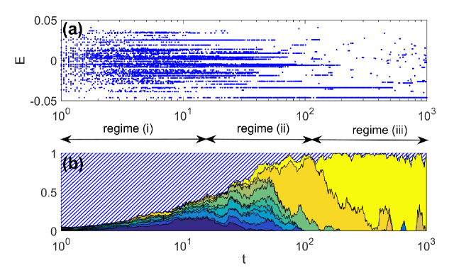
Figure 2: Evolution in the REM house-of-card model. (a) The energy of individuals. For clarity only 1 in 20 individuals is shown. (b) Evolution of the largest sub-populations, as in Fig. 1. Model parameters $M=500,\,N=2500,\,\mu=1/50$.

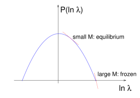
Figure 3: Equilibrium for the REM/House of Cards model.

Detailed Balance in the House-of-Cards model

For the House-of-Cards model, consider now for the successional mutation regime the ‘meta-dynamics’ of the dominant sub-population, considered as a single entity, neglecting the relatively short times in which the system is not concentrated into a single type (the fixation processess). Since in this example $\mu_{ij}=\mu_{ji}$:

$$\frac{P(i\to j)}{P(j\to i)}=\left(\frac{\lambda_{j}}{\lambda_{i}}\right)^{M-2}=e^{-(M-2)[\ln\lambda_{i}-\ln\lambda_{j}]}=e^{-\frac{M-2}{N}[E_{j}-E_{i}]}$$ (5)

This corresponds to a process with detailed balance and temperature $T=\frac{N}{M-2}$ and energies $E_{i}$ berg_adaptive_2004 ; berg_stochastic_2003 ; sella_application_2005 . If the symmetry is in mutation times $\tau_{ij}=\tau_{ji}$ the temperature becomes $T=\frac{N}{M-1}$. In what follows we focus on large $M$, and dropping $O\left(1/M\right)$ corrections we write $T=\frac{N}{M}$. At very long times, the system will reach a distribution

$$P({\mbox{dominant type at }}i)=\frac{e^{-E_{i}/T}}{\sum_{j}e^{-E_{j}/T}}$$ (6)

Still in the present model, finding the stationary distribution has been reduced to the solution of the equilibrium Random Energy Model derrida_random-energy_1980 , (see neher_emergence_2013 and cammarota_spontaneous_2014 ). In particular, we conclude that, depending on the value of $M$, at very long times the system will equilibrate to either a liquid phase (for $M/N<\ln 2$) or a ‘frozen’ phase (for $M/N>\ln 2$), see Fig. 3: in the former random extinction events stop the system from converging to the optimum level of fitness, while in the latter this level is at long times reached. A feature we find here, and is a general fact, is that even if the dynamics satisfy detailed balance, and are hence able in principle to equilibrate, this takes place at unrealistically long times.

The qualitative features of the population at different times has long been known, the similarity of the role played by fluctuations due to finite population size with thermal fluctuations has also been noted long ago peliti_introduction_1997 ; crow_introduction_1970 . Here the analogy becomes an identity, and features such as Muller’s ratchet – the accumulation of deleterious mutations in an irreversible manner – become just the question of an ordinary order-disorder phase transition. Similarly, the effect of population bottlenecks becomes the same as a spike in temperature.

Detailed Balance for non-symmetric mutation rates

Before concluding this section, let us note the result, valid for more general $\mu_{ij}$, but still satisfying (2) . In that case, the condition for detailed balance is berg_adaptive_2004 ; berg_stochastic_2003

$$1=\frac{P(i\to j)P(j\to k)P(k\to i)}{P(k\to j)P(j\to i)P(i\to k)}=\frac{\mu_{ij}\mu_{jk}\mu_{ki}}{\mu_{kj}\mu_{ji}\mu_{ik}}$$ (7)

meaning that the system satisfies detailed balance if the mutation probabilities $\mu_{ij}$ also do. The detailed balance condition (7) for them may be written: $\mu_{ij}=\hat{\mu}_{ij}e^{-\beta_{\tau}\hat{E}_{i}}$ for some $\hat{E}_{i}$ and $\hat{\mu}_{ij}=\hat{\mu}_{ji}$, and temperatures and energies become

$$T=\beta^{-1}=\frac{N_{s}}{M}\hskip 28.45274ptE_{i}=-N_{s}\ln\lambda_{i}+\frac{\beta_{\tau}}{\beta}\hat{E}_{i}$$ (8)

Throughout this paper we shall consider symmetric mutations $\mu_{ij}=\mu_{ji}$, so that $\beta_{\tau}=0$ and we recover $E_{i}=-N\ln\lambda_{i}$.

If a system evolves under a dynamics satisfying the detailed balance condition, it will after long times equilibrate to a distribution:

$$P_{eq}(i)={\cal N}e^{-\beta E_{i}}={\cal N}\;\lambda_{i}^{M}\;e^{-\beta\hat{E}_{i}}$$ (9)

the last factor being absent when $\mu_{ij}=\mu_{ji}$.

Limitations

The possibility of mapping evolutionary models to systems evolving in contact with a thermal bath seems very appealing as all the artillery of statistical mechanics: fundamental inequalities, analytic and numerical methods, fluctuation relations, immediately becomes available. It is for this reason surprising that the approach has received less attention than it deserves, even amongst physicists. This is probably due to a number of reasons, most importantly:

$\bullet$ The entire construction relies on a timescale-separation allowing for complete clustering (fixation) into a single-state population. In other words, the system has to be in the successional mutation regime.

$\bullet$ In the successional mutation regime, even if (meta)dynamics allows for equilibration, this will not realistically be reached before astronomical times. An equation like (6), and all the ones relying on it, will then not be applicable. In other words, the dynamics may be willing to equilibrate, but the times are short. The mapping will be at best with an out of equilibrium system in contact with a thermal bath.

As we shall see in what follows, the second objection brings in a solution of sorts to the first objection: because we have to necessarily deal with systems that are out of equilibrium at long times, a timescale-separation between processes that are fast and slow appears naturally (and inevitably). This separation may lead to detailed-balance, when generalized appropriately.

III A natural source of timescale-separation: the glassy element

In this section we briefly evoke the following fact: any long-time out of equilibrium system (as evolutionary systems will inevitably be) necessarily has fast and slow processes, the timescale separation growing with time.

Some physical systems do not equilibrate in experimental times, even if placed in contact with an equilibrium thermal bath. In practice, this means that equilibrium concepts such as temperature (of the sample) cannot be applied: two thermometers may measure different values depending on the way they are coupled to the system. On the other hand, the sample has an age, the time since it was prepared, that may affect its physical properties.

Three examples help clarify the different possibilities leading to time-scale separation. Consider first the case of diamond: it is actually a metastable state at room temperatures and pressures, there is always a probability of a sample decaying to graphite - the stable form of carbon. Despite its metastable, and hence nonequilibrium nature, while diamond lasts it behaves very much as an equilibrated system, only the decay itself would tell us otherwise. Next, consider the case of crystal ripening: the sample is constituted by an assembly of micro crystallites. Slowly but continuously, these grow one at the expense of the others, a process that only stops when the entire sample is a monocrystal. Nonequilibrium processes (the motion of crystal walls) are continuously happening, although ever more slowly. These processes coexist with the high-frequency vibrations within crystallites, which are essentially those of an equilibrium sample. Finally, consider the examples of glasses. These have no obvious ordered structure, but are constantly evolving to more and more equilibrated configurations. Once again, the high frequencies are just those of an equilibrated solid, while the slow processes are non-equilibrium, although in this case we have as yet no obvious way to picture them as we had with the example of crystallite growth.

In any one of these systems, we may define an autocorrelation function $C(t,t^{\prime})$, that measures how much the system evolves. It is defined to be $C(t,t^{\prime})=1$ if and only if the configurations are the same at $t$ and $t^{\prime}$, and falls to zero if they are completely uncorrelated. (We shall define a concrete $C(t,t^{\prime})$ for a model below). The fast and slow processes described above manifest themselves in a form of the autocorrelation as shown in Figure (4). There is a fast fall of the correlation to a plateau, corresponding to the vibrations that are insensitive to the out of equilibrium nature. At longer times, there is the slow relaxation ($\alpha$-relaxation, in the glassy jargon), that corresponds to the slow degrees of freedom. In long-time out of equilibrium systems the $\alpha$-relaxation time $t_{\alpha}$ becomes longer and longer as time passes, while the fast relaxations are rather insensitive to the overall time elapsed since preparation.

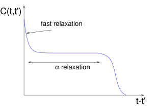
Figure 4: Timescale-separation

This fact (fast relaxations plus slower and slower $\alpha$ relaxations), is a completely generic feature, that one may consider true by definition: if there were only fixed timescales the system would be unchanged in time, i.e. in equilibrium. If we wish to picture this as a motion in phase space, two explanations are often given:

i) States: the system jumps discontinuously between valleys. While it is in a valley, its fluctuations are those of equilibrium, they are indifferent to the fact that the present valley is not the optimal one. It takes a time $t_{\alpha}$ to jump from a valley to another. Because the system optimizes, it becomes harder and harder to find new, deeper valleys, and $t_{\alpha}$ grows.

ii) Canyon: a rather abstract, but in fact more relevant mechanism in systems with many degrees of freedom is understood by considering the system evolving in a ‘canyon’, with many transverse directions that are essentially in equilibrium, while there is a slow drift along the canyon. This drift becomes slower and slower as time passes, partly because the dimensionality of the ‘canyon’ diminishes continuously – the number of ‘almost flat’ directions becomes smaller and smaller. This is exactly what happens in the ripening process, the slow directions being the coordinates that parametrize the (slowly disappearing) crystallite walls. This example is important, because it stresses the fact that fast and slow processes may happen simultaneously kurchan_phase_1996 .

We have already met timescale-separation in the previous example of the House of Cards model. Even if the mutation timescale $\tau$ is not very large, a time comes when the evolution slows down because it is very unlikely for a mutation to become favorable, and the population becomes essentially monoclonal (except for a ‘cloud’ of deleteriously mutated individuals, that itself depends on $\tau$). This slowing down due to a progressive difficulty in optimizing further is itself closely analogous to the situation in glassy systems. In the system with isolated states (Golf-course) one has that jumps become rarer and rarer, and hence dynamics slow on average, but a successful jump itself, when looked retrospectively, takes a short time. In this sense, the ”canyon” picture is quite different: the dynamics becomes slower, but there are, most of the times, no fast events. In fact, complex systems such as glasses exhibit the latter, rather than the former behavior. This will turn out to be relevant for our discussion here. Bearing these facts in mind, we now turn back to population dynamics.

IV Generalization to problems with fast and slow timescales: three examples

Aging systems automatically generate fast and slow timescales. For an aging evolutionary system, fast timescales will invalidate the approach that leads to detailed balance: there can be no clustering if there are fast successful mutations, that compete for fixation simultaneously. On the other hand, we expect that the slow timescales might yield some form of clustering, and hence of detailed balance, provided we coarse-grain over the short times. This section contains exercises to show that this is possible.

Successional regime in a picture with barrier crossing between ‘super-states’

We may first attempt to model a situation where there are ‘super-states’, each containing many states. Jumps between super-states become more and more infrequent, but there is no clustering in single states. The separation between timescales may come about in at least two ways:

$\bullet$ Because mutation probabilities probabilities are large between states belonging to the same super-state, and small otherwise.

$\bullet$ Because mutations between states within a superstate bring about changes of fitness that are much smaller than those allowed between different superstates.

Here we take as an example the former possibility. We consider the House of Cards just as before, but this time with ‘super-states’ $i$ with $i=1,...,2^{N}$, and, within each, states $(i,a)$ with $a=1,...,K_{i}$. The distribution of fitnesses is $\lambda_{ia}$. The timescale for jumps between states of different super-states $(i,a)\to(j,b)$ (with $i\neq j$) are large numbers $\tau_{ij}$, independent of $a$ and $b$. The timescale of jumps between configurations within a state $(i,a)\to(i,b)$ are much shorter $\tau_{o}\ll\tau$ . We shall assume that conditions are such that the population is most of the time clustered in a single super-state, but within a super-state it evolves fast (i.e. jumping fast between $(i,a)$ and $(i,b)$) and we may assume that the population is distributed according to a distribution $p_{ia}$. (This distribution need not, as we shall see, be the one corresponding to $M=\infty$, but it is not a thermal distribution either. In practice, it has to be calculated from first principles for given $M$). The total rate of reproduction within a super-state $i$ is then:

$$\bar{\lambda}_{i}\equiv\sum_{a}p_{ia}\lambda_{ia}$$ (10)

Assuming that rearrangements inside a super-state are rapid with respect to the time for a fixation from one super-state to another, we may take the average rates $\bar{\lambda}_{i}$.

It is easy to see that, under these conditions, detailed balance holds then for jumps between super-states. The role of fitness is played by an averaged value within each super-state. On the other hand, within a super-state jumps are fast and there is no clustering: the whole notion of thermal dynamics does not apply for this regime.

Diffusion in smooth fitness landscape

In the previous section, we described two explanations for the slow-down of dynamics. In explanation (i) above, slow dynamics result from motion in valleys, separated by barriers that are rarely crossed. Such an evolution corresponds to a Successional Mutation Regime, with additional mutations inside the valleys. The existence of detailed balance in this case, as well as the limitations on its validity, were illustrated with the example above. We now turn to discuss evolutionary dynamics as follows from explanation (ii), in which fast and slow evolutions coexist, and are not necessarily separated as in the case of discrete jumps between states. The problem we consider was treated in the literature twenty years ago: in a remarkable paper kessler_evolution_1997 all the details have been worked out, but no mention was made of how this implied a detailed balance relation in agreement with the one discussed above.

Figure 5: Traveling population pulse. $n\left(x\right)$ is the population distribution. Red arrow shows direction of average motion.

Consider a population of $M$ individuals performing simple diffusion along $x$ with diffusivity $D$, and reproducing (or dying) with a rate $\lambda(x)=e^{-N_{s}^{-1}E(x)}$ kessler_evolution_1997 . The offspring diffuses with a different realization of noise . It is clear that under such conditions no two individuals are in exactly the same position, except at the precise moment of birth. In fact, the population takes the form of a pulse of width $\Delta x=\sqrt{\frac{D}{\lambda}M}$, which represents a balance between spreading due to diffusion, and narrowing due to replication events. The pulse’s center of mass diffuses with the diffusivity $D_{pulse}$, and drifts with speed $=\kappa_{pulse}N_{s}\nabla\ln\lambda=-\kappa_{pulse}\nabla E(x)$ in the limit in which the variations of $E(x)$ are slow. For time-differences much longer than the relaxation time of the pulse, the system can be shown to obey a Langevin equation

$$\dot{x}=-\kappa\nabla E(x)+\eta(t)$$ (11)

where $\eta(t)$ can be taken to be a white noise $\langle\eta(t)\eta(t^{\prime})\rangle=D_{pulse}\delta(t-t^{\prime})$. For very small fitness gradients (see condition below), both $D_{pulse}$ and $\kappa_{pulse}$ have been calculated years ago. It was shown that zhang_diffusion_1990 ; meyer_clustering_1996 ; kessler_evolution_1997 $D_{pulse}=D$, and that kessler_evolution_1997 $\kappa_{pulse}=\left(M/N_{s}\right)D_{pulse}$, a fluctuation-dissipation relation with a corresponding inverse temperature $T^{-1}=M/N_{s}$. Remarkably, the dynamics satisfy detailed-balance exactly as in the very different regime of successional mutations, and with the same temperature, $T=M/N_{s}$. Here many concurrent mutations are allowed, thus relaxing the condition of successional mutations.

This detailed balance property holds if changes in log-fitness $\Delta\left(\ln\lambda\right)$ of an individual in a generation are small compared to $1/M$, or $\sqrt{D/\lambda}\nabla E(x)\ll N_{s}/M$. Noting that $\frac{d}{dt}\langle E\rangle=\frac{M}{N_{s}}D(\nabla E)^{2}$ we can rewrite this condition as $\frac{1}{\lambda}\frac{d}{dt}\langle E\rangle\ll N_{s}/M$, which is precisely a timescale separation – rate of average fitness improvement versus reproduction rate.

Unfortunately, the condition on the smallness of the gradient is quite restrictive. Indeed, the selective advantage (increment in log-fitness) of a single mutation must be smaller than $1/M$, which is unrealistic in many problems of cellular evolution. Outside this regime, for stronger fitness gradients, another regime is entered, studied in detail by Desai and Fisher, and by Rouzine et al. desai_beneficial_2007 ; rouzine_solitary_2003 ; rouzine_traveling-wave_2008 . When this regime holds, detailed balance is lost. As we now discuss, in problems with slow evolution in a high-dimensional rugged landscape, detailed-balance survives to regimes that contain both concurrent mutations, and larger fitness increments in a single mutation.

Smooth fitness landscape within a canyon

The model discussed above is a starting point for a ‘canyon’ model, where the slow direction in a canyon picture varies slowly and smoothly, while the fitness rapidly decreases in transverse directions. In this multi-dimensional model there are now two conditions for detailed balance to hold. First, in the slow direction we need $\frac{1}{\lambda}\frac{d}{dt}\langle E\rangle\ll N_{s}/M$ as in the one dimensional model. Secondly, the ‘cloud’ of deleterious mutations caused by mutation in fast directions must be small. (As for the successional regime, the condition is $\frac{\mu\lambda}{\lambda-\lambda_{del}}\ll 1$, where $\lambda,\lambda_{del}$ are the fitnesses in the pulse and the deleterious mutations, respectively.) Note that here the discreteness of the mutations in the fast directions is important, and cannot be replaced by a smooth landscape.

Detailed balance after temporal coarse-graining.

In the ‘super-state’ model, in smooth landscape picture, and its extension to a multi-dimensional ‘canyon’ model, detailed balance does not hold between individual states, as these change rapidly and in a non-thermal way. Instead, it holds for states when properly averaged over the population and a suitable time window. Let us see how this comes about. We consider a coarse-grained situation with ensembles of states $i$, with an average fitness given by $\bar{\lambda}_{i}$:

$$\bar{\lambda}_{i}\equiv\int_{t}^{t+\Delta}dt\sum_{a}\lambda_{a}\left(t\right)$$ (12)

where the sum runs over the population and time integrated over a time window $\Delta$ that is long compared to rapid fluctuations, but short compared to residence time in a super-state. In the smooth landscape model (and canyon model) the Einstein relation $\kappa_{pulse}=\left(M/N_{s}\right)D_{pulse}$ implies that between super-states

$$P(i\to j)=\tilde{\mu}_{ij}\;\frac{e^{\left(F_{j}-F_{i}\right)/N_{s}}-1}{e^{\left(M/N_{s}\right)(F_{j}-F_{i})}-1}$$ (13)

where $F_{i}\equiv-N_{s}\ln\bar{\lambda}_{i}$. Note that $F_{i}$ contains also the logarithm of the multiplicity, i.e. an entropic factor. Detailed balance then holds with

$$\frac{P(i\to j)}{P(j\to i)}=e^{-\left(M/N_{s}\right)\left(F_{j}-F_{i}\right)}$$ (14)

Detailed balance holds then for jumps between super-states. The role of energy is played by an averaged value within each super-state, together with the number of states within a super-state, leading to the free energy. On the other hand, within a super-state jumps are fast and there is no clustering: the whole notion of thermal dynamics does not apply. Given very long times, the system will eventually equilibrate. By this we mean that

$$P(clustering\;within\;super-state\;i)={\cal{N}}e^{-MF_{i}}$$ (15)

Let us emphasize that the distribution within this cluster is not given by a Boltzmann factor, and requires the full solution of the population dynamics within the super-state.

A Fluctuation Theorem

Consider a quantity $A_{ia}$ defined for each state. The average over a super-state $\bar{A}_{i}$ may be expressed as an average over a time $t_{in}$ sufficient to explore inside a state but short to move between super-states.

$$\bar{A}_{i}\sim\frac{1}{t}_{in}\int_{t}^{t+t_{in}}\;dt\;A_{ia}(t)$$ (16)

We also define $F_{i}^{h}=F_{i}-h\bar{A}_{i}$.

Assuming that the initial probability distribution of super-states is equilibrium with $h=0$ (Equation (15)) $P(i)\propto e^{-\beta F_{i}}$, we switch the field and wait for a time that is long with respect to the redistribution time inside a super-state, but otherwise arbitrary. The probability distribution of a change in the value of $\bar{A}$ is then $P(\Delta)$ which satisfies a Fluctuation Theorem

$$P(\Delta) = \sum_{ij}e^{-\beta F_{i}}P(i\to j)\delta[\Delta-(\bar{A}_{i}-\bar{A}_{j})]=\sum_{ij}e^{-\beta F_{i}^{h}}P(i\to j)e^{-\beta h\bar{A}_{i}}\delta[\Delta-(\bar{A}_{i}-\bar{A}_{j})]$$ (17)

$$= \sum_{ij}e^{-\beta F_{j}^{h}}P(j\to i)e^{-\beta h\bar{A}_{i}}\delta[\Delta-(\bar{A}_{i}-\bar{A}_{j})]=\sum_{ij}e^{-\beta F_{j}}P(j\to i)e^{-\beta h(\bar{A}_{i}-\bar{A}_{j})}\delta[\Delta-(\bar{A}_{i}-\bar{A}_{j})]$$

$$= e^{\beta h\Delta}P(-\Delta)$$

Note that this is valid even before the system had time to re-equilibrate at the new value of $h$, but it does require that there was equilibrium at $h=0$ at the outset. This is why the usefulness of this equation is rather limited in real life, although we will use it as a proof of principle in the next section.

V A model example

In this section we investigate how the above considerations apply to a model for which timescale-separation is not a feature put in ‘by hand’, but one that arises naturally. Our purpose is not to propose this model as a useful metaphor (there are many references on this, see for example pedersen_long_1981 ; sibani_evolution_1999 ; seetharaman_evolutionary_2010 ; saakian_eigen_2004 ; saakian_evolutionary_2009 ; saakian_solvable_2004 ), but rather work out the details in a nontrivial case. A complete analytic solution for the population dynamics in these models is perhaps possible, but seems like a daunting task.

We represent the internal state of the cell using Boolean variables. The fitness is a function on these variables, and the dynamics are a Moran process with selection and mutations. The fitness functions used are standard spin-glass benchmarks, whose landscape properties have been extensively studied kauffman_metabolic_1969 . The individual’s state is defined by ${\bf s}=\{s_{1},...,s_{N}\}$ variables taking values $0,1$. Fitness is constructed as follows: there are $\alpha N$ clauses $a$ with $K=3$ variables, of the form $(s_{i_{1}^{a}}\vee\overline{s_{i_{2}^{a}}}\vee s_{i_{3}^{a}})$ where both the $(i_{1}^{a},i_{2}^{a},i_{3}^{a})$ chosen for each clause – and the fact that the variable is negated or not – are decided at random once and for all. For example, Random K-SAT and Random Xor-SAT take the form:

OUTPUT = $(s_{18}\vee\overline{s_{3}}\vee s_{43})\wedge(s_{1}\vee s_{45}\vee\overline{s_{31}})...\wedge(\overline{s_{51}}\vee s_{7}\vee\overline{s_{8}})$   (SAT)

OUTPUT = $(s_{18}\veebar\overline{s_{3}}\veebar s_{43})\wedge(s_{1}\veebar s_{45}\veebar\overline{s_{31}})...\wedge(\overline{s_{51}}\veebar s_{7}\veebar\overline{s_{8}})$    (XorSAT)

If we assume that each clause has a multiplicative effect on the reproduction rate $\lambda$ , this takes us to an additive form for $E$

$$-\ln\lambda=\frac{1}{N}\sum_{a=1}^{\alpha N}[\mbox{error in clause }a]=\frac{1}{N}E$$ (18)

The factor $\frac{1}{N}$ sets the energy scale, that is we choose the scale $N_{s}=N$ (as in the House-of-cards example). Mutation time-scale $\tau_{0}=\left(\mu\lambda\right)^{-1}$ is taken equal for all mutations in a given simulation, and accordingly we make use of this variable throughout this section.

This problem is a standard benchmark of optimization theory, and has been extensively studied. We shall work in a regime with $\alpha=6$: for such a number of clauses the system virtually never has a solution where all clauses are satisfied, i.e. $E>0$. The landscape is rugged and the minima are separated and extremely hard to find.

We consider the dynamics of $M$ individuals, each identified by a vector ${\bf s}^{individual}$, performing diffusion by flipping randomly one of their components, reproducing or dying with fitness given by the SAT or XorSAT fitnesses. In other words, our ‘cells’ perform diffusion on the vertices of an $N$ dimensional hypercube (Fig 6), where they reproduce or die.

To obtain a meaningful phase-diagram (Fig 10), the scaling of $N_{s}$ and $\tau_{0}$ with growing $M$ must be consistently defined. We keep $M/N$ constant. To maintain the internal energy $E/N=-\ln\lambda$ unchanged, numerics show that mutation times must scale as $\tau_{0}=\tau M$, where $\tau$ is constant, for a given value of $M/N$. This entails that the width of the fitness distribution in the population at a given time is $\sigma_{\lambda}^{2}\sim\frac{M}{N_{s}^{2}\tau_{0}}\sim\frac{1}{M^{2}}$ (following arguments as in kessler_evolution_1997 ; ridgway_evolution_1998 ). The point-mutation time (i.e., time-scale for a given spin) is $\tau_{point}=N\tau_{0}$. This corresponds also to the time-scale for an individual to shuffle its entire genome.

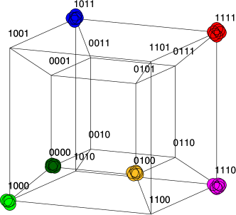
Figure 6: Genetic algorithm for SAT or XORSAT on the 4-dimensional hypercube. Each vertex has a given fitness value. Individuals reproduce with the rate determined by the vertex they are in, and mutate by diffusing to connected vertices.

Under conditions of the successional regime ($M/\left(\lambda\tau\right)\ll 1$), detailed balance would hold with temperature $T=\frac{N}{M}$. Indeed, in Fig. 7 we show the results of a simulated annealing performed with an ordinary Monte Carlo program on a single sample, superposed with a ‘populational annealing’ performed by slowly increasing the population of a set of individuals performing diffusion and reproducing according to the fitness in Eq. (18). Although this is not the main purpose of this paper, we note in passing that this ‘thermal’ analysis allows one to make an evaluation of such ‘genetic algorithms’ – in this case we understand that the Darwinian Annealing will have the same strengths and weaknesses as has Simulated Annealing. Furthermore, we see that allowing for large populations from the outset may be as catastrophic as is a sudden quench in an annealing procedure.

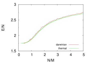
Figure 7: Thermal versus Darwinian annealing for XorSAT, for $\tau=16$. Similar results are obtained for K-SAT. Darwinian annealing is performed by controlling the population so that it increases slowly, at the same rate as in the corresponding thermal annealing.

In the limit $\tau\rightarrow\infty$, the population is fully clustered, and it behaves like a single realization of a SAT system, at temperature $T=\frac{N}{M}$. From what we know of the usual thermal XorSAT or SAT problem krzakala_gibbs_2007 , there is a (dynamic) glass transition below a certain temperature $T_{d}$. Below $T_{d}$ the phase-space breaks into components, and optimization becomes very hard. (This transition happens before the thermodynamic one, which itself is closely analogous to the freezing one of the REM). We may locate this transition by plotting the autocorrelation functions $C(t,t^{\prime})=\frac{4}{N}\sum_{i}(s_{i}\left(t\right)-\frac{1}{2})(s_{i}\left(t^{\prime}\right)-\frac{1}{2})$ at decreasing temperatures. As $T_{d}$ is approached from above, the correlation decays in a two-time process, a fast relaxation to a plateau followed by a much slower $\alpha$-relaxation taking a time $t_{\alpha}$. As $T_{d}$ is reached, $t_{\alpha}$ diverges. Below $T_{d}$, the system ages: the time $t_{\alpha}$ now keeps increasing with time, $C(t,t^{\prime})$ decays in a time $(t-t^{\prime})_{decay}\sim t_{\alpha}(t^{\prime})$ with $t_{\alpha}(t^{\prime})$ an increasing function of $t^{\prime}$.

What we have described is the ‘Random First Order Transition’ kirkpatrick_scaling_1989 . Nothing new here, as the system is equivalent to a thermal system, known to exhibit such a transition. Let us now consider smaller $\tau$, so that we no longer can assure that the $M$ individuals are fully clustered in a configuration at most times. We approach the transition by increasing $M$ at fixed $\tau$, and by decreasing $\tau$ at fixed $M$. The correlation curves obtained are shown in Fig (8), the nature of the transition remains the same, but the transition value of critical $M$ shifts with $\tau$.

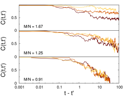
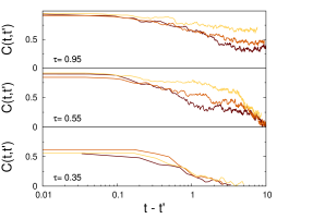
Figure 8: Values of the $C(t,t^{\prime})$ for a population crossing the glass transition from liquid (bottom) to glass (top). Values are $\tau=5$, $M/N={0.91,1.25,1.67}$ (left), and $M/N=4$, $\tau={0.35,0.55,0.95}$. The transition line is thus crossed by increasing $M$ or $\tau$, see the two arrows in fig. 10, the points corresponding to the figures are marked by crosses. The color code indicate the value of $\ln(t^{\prime})$, growing linearly from darker to lighter curves. In the top figures $t_{\alpha}$ grows as the system ages. Here and in all the following figures, the time is measured in units of (cell-)mutation times $\tau$ (i.e. a cell performs on average $O(N)$ flips in $\Delta t=O\left(1\right)$). The correlations are reasonably smooth, for a big system, even for a single run. This is evidence for a canyon, rather than “fast, rare jump” picture.

A confirmation of this is obtained by plotting the autocorrelation ‘noise’

$$\chi_{4}=N\left\langle\left[\frac{4}{N}\sum_{i}(s_{i}\left(t\right)-\frac{1}{2})(s_{i}\left(t^{\prime}\right)-\frac{1}{2})\right]^{2}\right\rangle-NC(t,t^{\prime})^{2}$$ (19)

a quantity that peaks at a level expected to diverge at the transition, at a time that we may estimate as $t_{\alpha}$, see Fig 9.

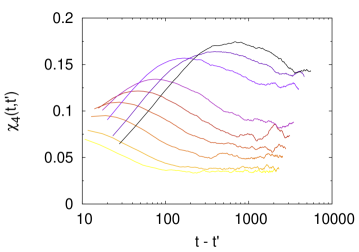
Figure 9: $\chi_{4}$ versus time on approaching the transition. Data shown for $M/N=1.4$, and a mutation rate $\tau^{-1}$ increasing linearly from 0.25 to 0.65 (bottom to top, dark to light curves). At lower mutations rates (not plotted) the glassy phase is reached, and the curves do not present any maximum and keep increasing with the waiting time $t$, as $t_{\alpha}$ is no longer defined.

Figure 10: Phase transition diagram in the $N/M$ vs $1/\tau$ plane. The transition line is given by the black circles, which correspond to the points where the value of the maximum in the $\chi_{4}$ function diverges, approaching the line by changing $M$ (filled circles) or $\tau$ (empty circles). The two arrows correspond to two possible crossing of the transition line, changing $\tau$ or $M$, the points indicated by a cross being those represented in Fig 8. Points labeled by numbers correspond to the situations of Fig 1, and indicate the parameters used in the verification of the averaged detailed balance, Fig 11.

All in all, we obtain the phase diagram of Fig 10. We know that the $\tau^{-1}=0$ axis is just equivalent to the thermal problem, with temperature $N/M$. What can we say about clustering for smaller $\tau$? Figure 1 shows the contributions of different configurations (the top uniform color corresponds to contributions smaller than 10% each). We see that for all but the highest $\tau$, the system is in the concurrent mutation regime desai_beneficial_2007 , and the thermal correspondence, applied naively, breaks down. Recalling previous sections, we still expect that whenever the $\alpha$ relaxation time is large (near and below the transition), the correspondence with a thermal system may still hold, but taken for quantities that are averaged over a state, and considering two situations at time-separations larger than $t_{\alpha}$.

A test of detailed balance in a region with large $\tau_{\alpha}$

Cheking detailed balance numerically is extremely hard. We shall here use the Fluctuation Theorem mustonen_fitness_2010 ; evans_fluctuation_2002 derived above, as an indirect test. Because this theorem requires to start from equilibrium, we are only in a position to do the test close to the glass transition, where the time-separation is large enough, but not within, because then equilibration becomes problematic. We thus place ourselves just above the transition (so that a stationary distribution might be reached) but not far from it (so that $t_{\alpha}$ is large), the circled numbers in Figure 10. We start with a system in equilibrium at time $t=0$, and we switch on a field $E\to E-hA$, where $A$ is any observable, in our case we choose $A=\sum_{i}s_{i}$. After an arbitrary time $t$ we measure again the value of $A$ and check the equation (see 17)

$$\ln{P[A(t)-A(0)=\Delta]}-\ln{P[A(t)-A(0)=-\Delta]}=\beta h\Delta$$ (20)

We obtain the plot Fig 11 (left), which does not verify the Fluctuation Theorem 20, except for very large $\tau$. This is what we expected, as there is no clustering into a single type, and the connection with a thermal system fails. Instead, when we compute the differences as $\Delta=\bar{A}(t)-\bar{A}(t=0)$, with $\bar{A}$ the average of $A$ within a window comparable to the time to reach a plateau – the ‘equilibration within a super-state’ time $\ll t_{\alpha}$ – and $t\sim 3t_{\alpha}$, the relation (20) for the averaged values $\Delta=\bar{A}(t)-\bar{A}(0)$ works perfectly, without fitting parameters. Note that below the transition line, the assumption of equilibration fails (at least for a large system); because of this, even if we expect detailed balance to hold for averaged quantities, the Fluctuation Relation does not apply

Finally, note that in our XorSAT simulations we have made two choices. First, we work with mutations that induce gradual jumps in the fitness (in sharp contrast, for example, with the House-of-cards model). Secondly, we chose the scale $N_{s}$ to be equal to the genome size $N$. As a result, individual mutations incur a change in fitness $\delta\lambda_{mut}\sim 1/M$. The jumps of $\delta\lambda_{mut}$ are larger than would allow for detailed balance to hold in a 1d step model, so a non-trivial extension of the known limiting conditions has been demonstrated. The scaling is the same as required by the step model, $\delta\lambda_{mut}\ll 1/M$, and therefore here we have not shown that the mutation steps can be parametrically larger (as a function of $M$). The population width in our simulations is $\sigma_{\lambda}\sim 1/M$, narrower than the minimum required for the step model: $\sigma_{\lambda}\sim M^{-1/2}$.

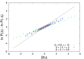
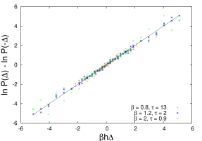
Figure 11: $\ln P(\Delta)-\ln P(-\Delta)$ versus $\beta h\Delta$, for close times and instantaneous values (left) and for quantities averaged over a time-window, and times separated by more than $t_{\alpha}$ (right). The latter works perfectly, without any fitting parameters. The parameters for the three curves, $(\beta,\tau)={(0.8,13),(1.2,2),(2,0.9)}$, correspond to those of figure 1, and are represented on the phase diagram of figure 10.

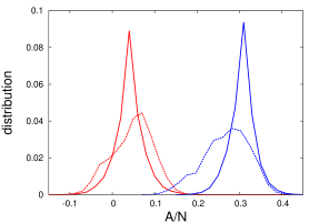
Figure 12: Instantaneous distribution of $A$ for two times, and for two time-windows of order $<t_{\alpha}$. The two sets are for two times separated by $3t_{\alpha}$. Fluctuations inside a state and between states are both larger than the instantaneous dispersion, underlying the fact that the distribution within a state is not the $M=\infty$ one predicted by the replicator equation.

VI Exploiting the correspondence

Let us discuss a few examples where the correspondence between thermal and population dynamics is exploited.

Replica-exchange / Parallel Tempering

It is a well known fact that evolution speeds up when small groups of individuals are in isolation from other groups hallatschek_genetic_2007 ; johnson_sewall_2008 . In the language of this paper, this is in direct analogy with warming up a complex system to make it anneal faster. Another related fact is the facilitation in development of antibiotic resistance by concentration gradients hermsen_rapidity_2012 . These two are extremely close to being evolutionary counterparts of more sophisticated equilibration procedures applied for complex systems. Consider the configuration of Fig. 13

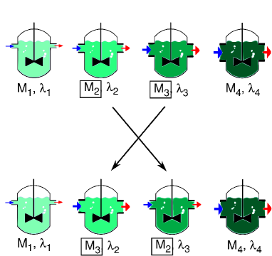
Figure 13: A series of chemostats with replica-exchange. Different population sizes are obtained by regulating the flow of medium.

The battery of chemostats are tuned to have increasing populations $M_{1}<M_{2}<M_{3}...$ If we are able to measure the reproduction rates of the cells, and exchange two chemostats with probability $\min\left\{\left(\frac{\lambda_{j}}{\lambda_{i}}\right)^{M_{i}-M_{j}};1\right\}$ we obtain the procedure known as Parallel Tempering earl_parallel_2005 . This is a well established procedure where several systems at different temperatures are evolved separately, and occasionally permuted following a rule analogous to the above. The interest is not only to accelerate evolution, but to do so in a manner that respects the thermal distributions, in our case the distributions associated with each population size. Thus the same final distribution is obtained, but it is reached faster.

An alternative way of implementing the same procedure is the following. Take two chemostats A and B, duplicate them into A’ and B’. Seed an individual of A’ into B’, and an individual of B’ into bottle A’. If both invading individuals are successful in fixing, replace the (A,B) by (A’,B’). Otherwise, discard (A’,B’) and continue with (A,B). One can show that the probabilities are the correct ones for Parallel Tempering, that is:

$$\frac{P(i:A\to B\mathrm{\ \ and\ \ }j:B\to A)}{P(i:B\to A\mathrm{\ \ and\ \ }j:A\to B)}=e^{(\beta_{i}-\beta_{j})(E_{i}-E_{j})}$$ (21)

Another version of Parallel Tempering is the ‘many fields’, rather than the ‘many temperature’ version. The systems are then all at the same temperature, but at different fields $h_{1}(S),h_{2}(S),...$. Exchange between two systems is accepted with the Monte Carlo rule. The analogue here is to use a series of chemostats with, for example, increasing concentrations of antibiotic, and make exchanges in concentrations according to the rule in the previous paragraph.

Kovacs effect

The Kovacs effect is a manifestation of the presence of processes with more than one relaxation timescale within an out-of-equilibrium system. The idea is to make the fast and slow processes ‘play against’ one another. Originally, it was discussed as a prove that a glass cannot be represented by a single extra parameter encapsulating all the history of temperature changes. To do this, Kovacs kovacs_transition_1964 considered two out of equilibrium situations with equal energy but with different previous histories, and showed that their subsequent evolutions are different. In our present case, the Kovacs effect shows that fitness need not increase, even when parameters are not changing.

In a glassy context mossa_crossover_2004 , the system is started in the liquid phase and quenched rapidly to very low temperatures. The glass so obtained evolves fast at first, but remains trapped in regions of relatively high energy from which it finds it hard to escape. Next, the system is taken to a higher, but still glassy, temperature. The immediate reaction is an increase in energy, because of the thermal agitation, but at later times the increased thermal activation allows the system to optimize more efficiently, and the energy decreases.

For a population, the Kovacs effect would proceed as follows. A system is put in a new, stressed situation. The population is allowed to grow fast as it adapts. Once population has reached high levels, new mutations become difficult to establish. If one then isolates a small subsystem, and keeps its size small, at first some bad mutations will decrease the fitness, but in the long run fitness should increase beyond what it was originally, thanks to the possibility of a small system to explore beneficial mutations. In Fig 14 we shows how this happens in our simple model. Another variant of the same is, instead of isolating a subensemble of the population, to consider a situation in which the individuals suddenly increase their mutation rate. The effect is similar, as shown in Fig. 15.

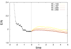
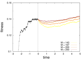
Figure 14: Energy (left) and fitness (right) evolutions following adaptation to a new situation, followed by a bottleneck. At some time $t<0$, the population is quenched to a very low temperature, $M_{q}=1000$, and let relax (black solid line). At time $t=0$ (vertical dashed line) the population is reduced instantaneously to a lower M = {143, 167, 200, 250} (lighter to darker lines). The fast timescale re-adaptation causes, in the short period, the energy (resp. fitness) to increase (resp. decrease). However, on longer timescales, the smaller size of the population allows it to explore more efficiently the energy (fitness) landscape, finding more favourable configurations.

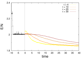
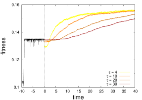
Figure 15: Energy and fitness evolutions following an increase in mutation rate. The population is let evolve at a low mutation rate, $\tau=40$ (black solid line). At time $t=0$ (vertical dashed line) the mutation rate is instantaneously increased, to value $\tau={4,10,20,30}$ (lighter to darker lines). Again, the interplay between fast and slow timescale causes the energy (resp. fitness) to increase (resp. decrease) at first, to then decrease (increase) in the long run.

More complex cycles

Kovacs’ effect is relatively simple. There are other effects in glassy systems that are highly nontrivial, and have only been observed after a very educated (by theory) guess stimulated the experiment with spin glasses. The experimental protocol jonason_memory_1998 is sketched in Fig 16. In the ‘writing period’ the temperature is slowly decreased starting from the high temperature phase down to very low temperature, but stopping for relatively long times in an intermediate temperature and waiting before resuming the decrease. After reaching the lowest temperature, one starts the ‘reading’ period, which consists of a slow increase in temperature, while measuring at the same time any quantity that may yield information of the ‘age’ of the sample, in the case of spin glasses the response to a low-frequency a.c. field (which becomes smaller as time passes). The surprising fact is that when the temperature during the ‘reading phase’ traverses the value at which there was a stop in the ‘writing phase’, there is a dip in the response to an a.c. field – an indication of being ‘older’ at that temperature: as if the system could age independently at different temperatures. This may be even generalized to several stops, which are memorized independently. It is easy to propose a similar experiment for a population, made to grow slowly, with stops at different ‘bottlenecks’. Different subsamples of different sizes extracted from the large population would bear memory of past history, subsample sizes corresponding to bottleneck sizes that happened in the past would show measurable differences in their successful mutation rates (they should be smaller) with subsamples whose size does not correspond to bottleneck sizes undergone in the past.

We have not attempted to simulate this here, because no successful simulation has ever been performed yet for this model, even in the original thermal context, probably due to size and time constraints in the numerical power.

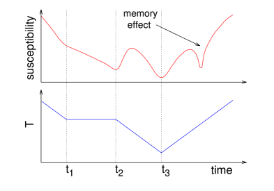
Figure 16: The experimental protocol of jonason_memory_1998 . A procedure of annealing is carried on until $t=t_{1}$. Then, while $t_{1}<t<t_{2}$ the system is allowed to relax, while the temperature is keep fixed to $T_{w}$. The annealing is then resumed up to a time $t_{3}$. The system is subsequently subjected to a smooth increase in temperature: as the temperature passes through $T=T_{w}$ a drop in the susceptibility is observed, showing memory of the annealing that had taken place at that temperature.

Changing environments: connection to glassy rheology

A system as the one we are considering, which is achieving better fitness by slowly adapting to a complex landscape, is extremely sensitive to changes in this landscape. This effect has been discussed in mustonen_molecular_2008 , although in a slightly different form, and also in kussell_phenotypic_2005 . The counterpart in glass physics of this fact has long been known. Consider the situation struik_rejuvenation_1997 of a plastic bar prepared a time $t_{w}$ ago from a melt. The polymers constituting the bar slowly rearrange – ever more slowly – to energetically better and better configurations, and this process is known to go on at least for decades. The bar is out of equilibrium, a fact that we may recognize by testing its response to stress, which measurably depends on $t_{w}$. Now suppose that we apply a large, fixed deformation to the bar, for example applying a strong torsion one way and the other. The new constraints change the problem of optimization the polymers are ‘solving’: we expect evolution to restart to a certain extent, and the apparent ‘age’ of the bar to become smaller than $t_{w}$. This is indeed what happens struik_rejuvenation_1997 , a phenomenon called ‘rejuvenation’. Rejuvenation brings about an acceleration in the dynamics. If the changes are continuous and different, instead of aging (growth of $t_{\alpha}$), the system settles in a value of $t_{\alpha}$ that depends on – adapts to – the speed of change of the energy landscape. Note that this property of evolution speed adapting to landscape change speed, that is often attributed to a form of criticality kauffman_metabolic_1969 , here it appears as a universal property of aging systems.

Applying the same logic to our model, one expects a similar result. In order to model the changes in fitness landscape, we change at fixed intervals of time a randomly chosen clause, for example by changing the identity of one of the intervening Boolean variables (a slight change in the fitness function). For different rates of change, we plot the ‘age’ of the system, as measured by $\chi_{4}$. The results are shown on Figure 17: if the environment is randomly changing, the system evolves to accommodate various conditions, and time-scales for changes in the environment are reflected in the time-scales for changes inside system.

Although we shall not pursue this line here, let us remark that one need not consider only random changes of fitness landscape, but also repetitive ones. Recently, Fridman et al fridman_optimization_2014 subjected bacterial populations to intermittent exposure to antibiotics. All strains adapted via phenotypic changes and developed of tolerance by adjusting the lag time of bacteria before regrowth to match the duration of the antibiotic-exposure interval. In other words, the system adapted to the cycle itself. Correspondingly, in another recent paper, Fiocco et. al. fiocco_encoding_2014 have studied the effect of letting evolve a glassy system under the influence of a periodic field, strong enough to affect substantially its evolution. The system ‘adapts’ to this non-stationary situation, just as it would to a stationary field: subjecting further the sample to new cycles of different amplitudes (‘reading’) one may easily distinguish the cycle at which it has been optimized (‘writing’).

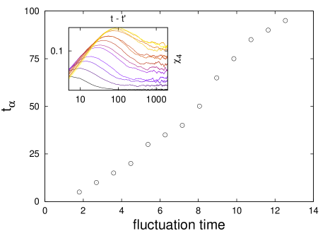
Figure 17: $\alpha$-time versus speed of variation of fitness landscape. Inset: $\chi_{4}$ versus time for different speeds of random variation of landscape (darker curves correspond to faster variations). The $t_{\alpha}$ value for each point of the main figure is the time at which the corresponding curve reaches its maximum, a measure of the $\alpha$-time.

VII Discussion

Let us discuss here the domain of validity of the mapping into a thermal system. The first element we have assumed throughout, is the fact that the population is composed of individuals that do not interact, except through a mechanism that limits the total population size. More general settings could include the situation where the limited resource is space, as in the case of cells growing in a Petri dish. It is not impossible that generalizations in this direction can be made.

We have lifted the assumption of successional mutations. The price we pay is the fact that the thermal approach is then only valid for the slow evolution; for the fast mutations, the detailed balance property does not hold. The advantage is that now the approach is valid to any system evolving through random drift and selection if the fitness landscape is complex enough, so that the optimum is not reached in reasonable times, and evolution slows down.

The most general conditions for our extended detailed balance to hold are not yet known, and will require further investigation. Mutation probabilities (the $\mu_{ij}$) need to satisfy a symmetry property, Eq. (7), for detailed balance to hold. If, on the contrary, the mutation dynamics at the level of the individuals contains cycles, the detailed balance property will be violated. Two things may happen: either the cycles persist even for the slow timescales (so that there are closed cycles of slow mutations), or they do not. In the latter case slow dynamics would still be thermal.

As was mentioned in several places, we must give up the property of equilibrium, which is not realistic even when detailed balance holds. We are left with a system that is in fact like a glass: it works its way towards equilibrium while external conditions do not change, but never achieves it. Such systems have their own properties and rules. We have now a much better understanding of them, and there is the potential that many of the features that we have encountered in studying glasses may be applied to evolving populations with strong epistasis.

- (1) J. F. Crow and M. Kimura, “An introduction to population genetics theory,” pp. xiv+591 pp., 1970.
- (2) L. Peliti, “Introduction to the statistical theory of Darwinian evolution,” arXiv:cond-mat/9712027, Dec. 1997, arXiv: cond-mat/9712027.
- (3) L. S. Tsimring, H. Levine, and D. A. Kessler, “RNA virus evolution via a fitness-space model,” Physical review letters, vol. 76, no. 23, p. 4440, 1996.
- (4) M. Lynch, “The Lower Bound to the Evolution of Mutation Rates,” Genome Biol Evol, vol. 3, pp. 1107–1118, Jan. 2011.
- (5) R. A. Neher, M. Vucelja, M. Mezard, and B. I. Shraiman, “Emergence of clones in sexual populations,” Journal of Statistical Mechanics: Theory and Experiment, vol. 2013, no. 01, p. P01008, Jan. 2013.
- (6) G. Sella and A. E. Hirsh, “The application of statistical physics to evolutionary biology,” PNAS, vol. 102, no. 27, pp. 9541–9546, Jul. 2005.
- (7) V. Mustonen and M. Lassig, “Fitness flux and ubiquity of adaptive evolution,” PNAS, vol. 107, no. 9, pp. 4248–4253, Mar. 2010.
- (8) A different form of detailed-balance holds when the equilibrium distribution can be factorized in terms of allele frequencies (linkage equilibrium) [See Supp.Mat. of mustonen_fitness_2010 ]. We do not discuss this further, as we are here primarily interested in cases with rugged fitness landscapes associated with strong interactions (epistasis).
- (9) J. Berg and M. Lassig, “Stochastic evolution of transcription factor binding sites,” Biophysics, vol. 48, no. 1, pp. 36–44, 2003.
- (10) J. Berg, S. Willmann, and M. Lassig, “Adaptive evolution of transcription factor binding sites,” BMC Evolutionary Biology, vol. 4, no. 1, p. 42, Oct. 2004.
- (11) N. H. Barton and J. B. Coe, “On the application of statistical physics to evolutionary biology,” Journal of Theoretical Biology, vol. 259, no. 2, pp. 317–324, Jul. 2009.
- (12) S. F. Elena and R. E. Lenski, “Microbial genetics: Evolution experiments with microorganisms: the dynamics and genetic bases of adaptation,” Nature Reviews Genetics, vol. 4, no. 6, pp. 457–469, Jun. 2003.
- (13) P. A. P. Moran, The Statistical Processes of Evolutionary Theory. Clarendon Press, 1962.
- (14) M. A. Nowak, Evolutionary Dynamics. Harvard University Press, Sep. 2006.
- (15) M. M. Desai and D. S. Fisher, “Beneficial Mutation-Selection Balance and the Effect of Linkage on Positive Selection,” Genetics, vol. 176, no. 3, pp. 1759–1798, Jul. 2007.
- (16) I. M. Rouzine, J. Wakeley, and J. M. Coffin, “The solitary wave of asexual evolution,” PNAS, vol. 100, no. 2, pp. 587–592, Jan. 2003.
- (17) I. M. Rouzine, Ã. Brunet, and C. O. Wilke, “The traveling-wave approach to asexual evolution: Muller’s ratchet and speed of adaptation,” Theoretical Population Biology, vol. 73, no. 1, pp. 24–46, Feb. 2008.
- (18) B. H. Good, I. M. Rouzine, D. J. Balick, O. Hallatschek, and M. M. Desai, “Distribution of fixed beneficial mutations and the rate of adaptation in asexual populations,” PNAS, vol. 109, no. 13, pp. 4950–4955, Mar. 2012.
- (19) V. Mustonen and M. Lassig, “Molecular Evolution under Fitness Fluctuations,” Physical Review Letters, vol. 100, no. 10, Mar. 2008.
- (20) B. Derrida, “Random-Energy Model: Limit of a Family of Disordered Models,” Phys. Rev. Lett., vol. 45, no. 2, pp. 79–82, Jul. 1980.
- (21) C. Cammarota and E. Marinari, “Spontaneous energy-barrier formation in an entropy-driven glassy dynamics,” arXiv:1410.2116 [cond-mat], Oct. 2014, arXiv: 1410.2116.
- (22) J. Kurchan and L. Laloux, “Phase space geometry and slow dynamics,” J. Phys. A: Math. Gen., vol. 29, no. 9, p. 1929, May 1996.
- (23) D. A. Kessler, H. Levine, D. Ridgway, and L. Tsimring, “Evolution on a smooth landscape,” J Stat Phys, vol. 87, no. 3-4, pp. 519–544, May 1997.
- (24) Y.-C. Zhang, M. Serva, and M. Polikarpov, “Diffusion reproduction processes,” J Stat Phys, vol. 58, no. 5-6, pp. 849–861, Mar. 1990.
- (25) M. Meyer, S. Havlin, and A. Bunde, “Clustering of independently diffusing individuals by birth and death processes,” Phys. Rev. E, vol. 54, no. 5, pp. 5567–5570, Nov. 1996.
- (26) J. B. Pedersen and P. Sibani, “The long time behavior of the rate of recombination,” The Journal of Chemical Physics, vol. 75, no. 11, pp. 5368–5372, Dec. 1981.
- (27) P. Sibani and A. Pedersen, “Evolution dynamics in terraced NK landscapes,” EPL, vol. 48, no. 3, p. 346, Nov. 1999.
- (28) S. Seetharaman and K. Jain, “Evolutionary dynamics on strongly correlated fitness landscapes,” Phys. Rev. E, vol. 82, no. 3, p. 031109, Sep. 2010.
- (29) D. Saakian and C.-K. Hu, “Eigen model as a quantum spin chain: Exact dynamics,” Phys. Rev. E, vol. 69, no. 2, p. 021913, Feb. 2004.
- (30) D. B. Saakian and J. F. Fontanari, “Evolutionary dynamics on rugged fitness landscapes: Exact dynamics and information theoretical aspects,” Physical Review E, vol. 80, no. 4, Oct. 2009.
- (31) D. B. Saakian and C.-K. Hu, “Solvable biological evolution model with a parallel mutation-selection scheme,” Phys. Rev. E, vol. 69, no. 4, p. 046121, Apr. 2004.
- (32) S. A. Kauffman, “Metabolic stability and epigenesis in randomly constructed genetic nets,” Journal of Theoretical Biology, vol. 22, no. 3, pp. 437–467, Mar. 1969.
- (33) D. Ridgway, H. Levine, and D. A. Kessler, “Evolution on a Smooth Landscape: The Role of Bias,” Journal of Statistical Physics, vol. 90, no. 1-2, pp. 191–210, Jan. 1998.
- (34) F. Krzakala, A. Montanari, F. Ricci-Tersenghi, G. Semerjian, and L. Zdeborova, “Gibbs states and the set of solutions of random constraint satisfaction problems,” PNAS, vol. 104, no. 25, pp. 10 318–10 323, Jun. 2007.
- (35) T. R. Kirkpatrick, D. Thirumalai, and P. G. Wolynes, “Scaling concepts for the dynamics of viscous liquids near an ideal glassy state,” Physical Review A, vol. 40, no. 2, p. 1045, 1989.
- (36) D. J. Evans and D. J. Searles, “The Fluctuation Theorem,” Advances in Physics, vol. 51, no. 7, pp. 1529–1585, Nov. 2002.
- (37) O. Hallatschek, P. Hersen, S. Ramanathan, and D. R. Nelson, “Genetic drift at expanding frontiers promotes gene segregation,” PNAS, vol. 104, no. 50, pp. 19 926–19 930, Dec. 2007.
- (38) N. Johnson, “Sewall wright and the development of shifting balance theory.” Nature Education, vol. 1, no. 52, 2008.
- (39) R. Hermsen, J. B. Deris, and T. Hwa, “On the rapidity of antibiotic resistance evolution facilitated by a concentration gradient,” PNAS, vol. 109, no. 27, pp. 10 775–10 780, Jul. 2012.
- (40) D. J. Earl and M. W. Deem, “Parallel tempering: Theory, applications, and new perspectives,” Physical Chemistry Chemical Physics, vol. 7, no. 23, p. 3910, 2005.
- (41) A. J. Kovacs, “Transition vitreuse dans les polymeres amorphes. Etude phenomenologique,” in Fortschritte Der Hochpolymeren-Forschung, ser. Advances in Polymer Science. Springer Berlin Heidelberg, 1964, no. 3/3, pp. 394–507.
- (42) S. Mossa and F. Sciortino, “Crossover (or Kovacs) Effect in an Aging Molecular Liquid,” Physical Review Letters, vol. 92, no. 4, Jan. 2004.
- (43) K. Jonason, E. Vincent, J. Hammann, J. P. Bouchaud, and P. Nordblad, “Memory and chaos effects in spin glasses,” Physical Review Letters, vol. 81, no. 15, p. 3243, 1998.
- (44) E. Kussell and S. Leibler, “Phenotypic Diversity, Population Growth, and Information in Fluctuating Environments,” Science, vol. 309, no. 5743, pp. 2075–2078, Sep. 2005.
- (45) L. C. E. Struik, “On the rejuvenation of physically aged polymers by mechanical deformation,” Polymer, vol. 38, no. 16, pp. 4053–4057, Aug. 1997.
- (46) O. Fridman, A. Goldberg, I. Ronin, N. Shoresh, and N. Q. Balaban, “Optimization of lag time underlies antibiotic tolerance in evolved bacterial populations,” Nature, vol. 513, no. 7518, pp. 418–421, Sep. 2014.
- (47) D. Fiocco, G. Foffi, and S. Sastry, “Encoding of Memory in Sheared Amorphous Solids,” Phys. Rev. Lett., vol. 112, no. 2, p. 025702, Jan. 2014.