Assessment of petrophysical quantities inspired by joint multifractal approach

Abstract

In this paper joint multifractal random walk approach is carried out to analyze some petrophysical quantities for characterizing the petroleum reservoir. These quantities include Gamma emission (GR), sonic transient time (DT) and Neutron porosity (NPHI) which are collected from four wells of a reservoir. To quantify mutual interaction of petrophysical quantities, joint multifractal random walk is implemented. This approach is based on the mutual multiplicative cascade notion in the multifractal formalism and in this approach $L_{0}$ represents a benchmark to describe the nature of cross-correlation between two series. The analysis of the petrophysical quantities revealed that GR for all wells has strongly multifractal nature due to the considerable abundance of large fluctuations in various scales. The variance of probability distribution function, $\lambda_{\ell}^{2}$, at scale $\ell$ and its intercept determine the multifractal properties of the data sets sourced by probability density function. The value of $\lambda_{0}^{2}$ for NPHI data set is less than GR’s, however, DT shows a nearly monofractal behavior, namely $\lambda_{0}^{2}\rightarrow 0$, so we find that $\lambda_{0}^{2}({\rm GR})>\lambda_{0}^{2}({\rm NPHI})\gg\lambda_{0}^{2}({\rm DT})$. While, the value of Hurst exponents can not discriminate between series GR, NPHI and DT. Joint analysis of the petrophysical quantities for considered wells demonstrates that $L_{0}$ has negative value for GR-NPHI confirming that finding shaly layers is in competition with finding porous medium while it takes positive value for GR-DT determining that continuum medium can be detectable by evaluating the statistical properties of GR and its cross-correlation to DT signal.

Keywords: Multifractal Random Walk, Joint Multifractal Parameter, Non-Gaussian Probability Density Function, Cross-Correlation Function.

I Introduction

Undoubtedly, petroleum, gas and fossil fuels have most important impact on economics, social life and associated industries laz12 . In the research of oil and gas fields, petrophysical quantities are analyzed in order to determine the economic benefit of oil fields and gas production and consequently on decision what equipments are useful to improve the extract and/or production efficiency of underlying wells. For a typical reservoir the characteristics such as thickness (bed boundaries), lithology containing information about rock type, porosity, fluid saturations, fluid identification and permeability, pressure and fractional flow involving gas, oil and water should be quantify as accurately as possible. There are several indicators to explore and analyze oil and gas reservoirs ellis87 ; datalog99 ; hea00 ; rashed11 . We are not able to extract full information from them without understanding how they are affected by each others. These indicators possess a non-Gaussian behavior due to the fact that the density of oil wells depend on depth of reservoirs. By getting close to oil reservoir a gradient in the medium is observed. This kind of non-Gaussianity could be a sign of medium changes and/or an indicator of reservoir approaching. Prospect benchmarks in such system are not only coupled but also may be non-Gaussian. In order to take into account both mentioned properties in a typical system, simultaneously, the generalized multifractal random walk can be a proper method to implement Bacry ; Muzy1 ; Bacry1 ; Muzy2 .

The multifractal formalism introduced in the theory of complex systems and nonlinear dynamics has been applied in various fields of researches ranging from biology and finance e.g. foreign exchange rates Ghas96 , stock index Kiy06 ; Sadegh , human heartbeat fluctuations Kiy004 , seismic time series Tabar09 ; Telesca0 ; Telesca1 , sol-gel transition Shayeganfar2 , non-equilibrium growth processes vicsek ; barabashi and solar and wind energies Sorrise ; Telesca to climate and metrology climate1 ; climate2 ; climate3 ; climate4 ; sadeghriver . However the notion of multifractality, is widely used in many of above researches, but there are different approaches to characterize this concept in such systems from complexity point of view.

Multifractal models have been developed inspired by turbulent cascades in hydrodynamic turbulence in which multiplicative cascades display scale-invariant statistical properties Frisch . In the context of multiplicative random cascades Meneveau1 ; halsey ; palad ; Meneveau , recently Bacry et al. introduced multifractal random walk model as a continuous random walk with the logarithm of the correlated stochastic variances Bacry ; Muzy1 ; Bacry1 . The occurrence of large fluctuations in a typical system leads to a log-normal deviation from the normal shape of probability density function. Consequently, multifractality is imposed in such system sourced by deviation from Gaussian PDF. The mutual interaction between various fluctuations in linear and non-linear regimes are of interest, so in order to examine such property, Muzy et al. Muzy2 demonstrated a generalization of univariate multifractal random walk to a multivariate framework which is so-called multivariate multifractal random walk.

In this paper we follow the research done by Z. Koohi et. al. koohi , and rely on joint multifractal random walk approach to make more complete our knowledge concerning petrophysical data sets. In koohi , authors examined the shape of probability distribution function (PDF) of underlying quantity in the framework of multiplicative random cascades. Also the changing shape of PDF with chosen scale, namely from dissipation to large scales, has been characterized by finding the scale dependency of $\lambda^{2}$ denoted by $\lambda_{\ell}^{2}$. The so-called non-Gaussian factor, $\lambda_{\ell}^{2}$, characterizes the non-Gaussianity of corresponding PDF. In turbulence this quantity deals with number of Cascades naert1 ; naert2 . From thermodynamics point of view, $\lambda_{\ell}^{2}$ is potentially related to partition function, therefore free energy of system can be pertinent as: $F=-k_{\beta}T\ln(\lambda_{\ell}^{2})$ novikov . In addition, parameter $\lambda_{\ell}^{2}$ represents fluctuations of the variances based on the notion of log-normal multiplicative processes. This means that, the larger $\lambda_{\ell}^{2}$, the higher probability of finding higher values of fluctuation in underlying quantity. Besides mentioned investigations, the mutual correlation between various petrophysical surveys have been motivated from statistical properties point of view. To this end, joint multifractal random walk will be implemented to examine cross-correlation properties.

The quantities investigated in this research include Gamma emission, (GR), sonic transient time, (DT), and Neutron porosity, (NPHI) ellis87 ; datalog99 ; hea00 ; Leite ; Montagne ; Christie ; koohi12 ; Fedi ; log1 ; log2 . Each of mentioned data contains valuable information about the underlying reservoir. GR is capable to give proper estimation concerning radioactive components existing in reservoir rocks. NPHI belongs to category of nuclear logging providing some information about porosity and lithology and has been established on migration length and bulk capture cross-section. Our results obtained from four wells of the reservoir confirmed that GR has strongly multifractal behavior due to the considerable abundance of large scale fluctuations in this quantity. The value of $\lambda_{0}^{2}$ ($\lambda_{0}^{2}$ is intercept of $\lambda_{\ell}^{2}$ versus $\ell$) for NPHI data set is less than GR’s, however, DT shows a nearly monofractal behavior ($\lambda_{0}^{2}\rightarrow 0$). From joint analysis point of view, our results represent that $L_{0}=L_{\ell\to 0}$ for GR-NPHI pair has negative value while a positive value of $L_{0}$ for GR-DT pair is attained. To make theoretical prediction for scaling exponents computed by multifractal random walk and its joint method, we also apply adaptive detrending method to remove probable trends superimposed on data and clean date will be used for Detrended Fluctuation Analysis (DFA) to determine corresponding Hurst exponent. This exponent is used for deriving theoretical prediction of scaling exponents derived in context of multifractal random walk.

The rest of this paper is organized as follows: In sections II and III, we describe multifractal random walk model and joint multifractal random walk, respectively. In section IV, Adaptive detrending algorithm followed by Detrending Fluctuation Analysis are explained. In section V we explain the data sets and the location where they have been recorded. Section VI is devoted to analyze the petrophysical data sets. Summary and conclusion are given in section VII.

II Multifractal model

In this section we rely on multifractal approach to model the underlying data set. Self-similarity and self-affinity can be assigned to many observed shapes as well as processes in nature. This geometrical index was introduced for the first time by Mandelbrot Feder . The particular characteristic concerning fractal and multifractal phenomena is scaling behavior. Assume a typical stochastic fluctuation recorded during an experiment or simulation as a function of dynamical parameter (spatial or temporal) represented by $x(t)$. One of scale invariant properties of mentioned stochastic series is generally demanded by $\xi_{q}$ as follows Bacry :

$$m(q,\ell) \equiv \sum_{t}\mid x(t+\ell)-x(t)\mid^{q}$$ (1)

$$= \mathcal{A}_{q}\ell^{\xi_{q}}$$ (2)

here $\mathcal{A}_{q}$ is a prefactor and $\xi_{q}$ corresponds to the exponent of power law function. If the exponent $\xi_{q}$ is a linear function versus $q$, namely $\xi_{q}=Hq$, a single Hurst exponent, $H$, is adequate to characterize the fractal property of underlying signal and $x(t)$ is called monofractal. While for a nonlinear dependence of $\xi_{q}$ with respect to $q$, $x(t)$ belongs to multifractal category. It must point out that the range of scaling regime might be given as a prior, namely for turbulence, it is less than characteristic scale in fully developed turbulence. For arbitrary fluctuation, mentioned length (time) scale is considered about correlation length (time) scale. According to physics of turbulence, it has been demonstrated that for small Reynolds number, the inertial range is very small and the scaling behavior described by Eq. (1) is either absent or difficult to observe Gao . Therefore, in a general process, this case may occur. The concept of extended self-similarity provides a solution to this problem. Benzi et al. found that the scaling properties of the velocity increments can be extended up to the dissipation range if we modify Eq. (1) as : $m(q,\ell)\sim m(3,\ell)^{\zeta_{q}}$ Benzi . For fractal processes $m(3,\ell)\sim\ell^{3H}$ then $\zeta_{q}=\frac{q}{3}$. The relation between $\xi_{q}$ as well as $\zeta_{q}$ and the non-Gaussian parameter in the hierarchical multiplicative cascade model developed for the first time by Castaing et al. Castaing . In this robust approach the multifractality is assigned to PDF of underlying data set frisch97 ; Mandelbrot ; Kahane ; Meneveau ; Hentschel . Suppose that the increment of fluctuations at scales $\ell$ and $\beta\times\ell\ (\beta<\ell)$ can be modeled through the cascading rule:

$$[x(t+\beta\times\ell)-x(t)]=W_{\beta}[x(t+\ell)-x(t)],\quad\forall\ \ell,\beta>0$$ (3)

here $W_{\beta}$ is a stochastic variable depending only on $\beta$ and, behaves as a logarithmic infinitely divisible law Castaing ; Arneodo2 . Hereafter, for convenient, we use, $\delta_{\beta\times\ell}x(t)\equiv[x(t+\beta\times\ell)-x(t)]$ and $\delta_{\ell}x(t)\equiv[x(t+\ell)-x(t)]$. In addition, the integral form of the corresponding PDF at scale $\ell$ using its increment at scale $\beta\times\ell(\beta<\ell)$ can be written as Castaing :

$$P_{\ell}(\delta_{\ell}x)=\int G_{\ell,\beta\times\ell}(u)e^{-u}P_{\beta\times\ell}(e^{-u}\delta_{\ell}x)du$$ (4)

This equation states that PDF of $\delta_{\ell}x$ at a given scale, $\ell$, is determined as a weighted sum of PDF at a larger scale, $\beta\times\ell$. The shape of weight function, $G_{\ell,\beta\times\ell}(u)$, is determined by statistical nature of underlying data. As an example, for a self-similar kernel with a given Hurst exponent, the shape of kernel reads as $G_{\ell,\beta\times\ell}(u)=\delta_{D}(u-H\ln(\ell/(\beta\times\ell)))$. Here $\delta_{D}$ is Dirac delta function. Subsequently, $P_{\ell}(\delta_{\ell}x)\sim\beta^{H}P_{\beta\times\ell}(\beta^{H}\delta_{\ell}x)$ which is known as a geometrical convolution between the kernel $G_{\ell,\beta\times\ell}$ and $P_{\beta\times\ell}$ Muzy1 . Eq. (4) enables us to calculate $q$th order of absolute moment, $m(q,\ell)$ by determining the functional form of kernel. Any deviation from Dirac delta function for kernel leads to a deviation from pure Gaussian function for $P_{\ell}(\delta_{\ell}x)$. In this case underlying data has multifractal nature, consequently, the corresponding $\xi_{q}$ deviates from the linear behavior versus $q$. Inspired by fully developed turbulent flows by Castaing et. al. Castaing , one can find various stochastic variables which their PDFs are the same as that of given by Eq. (4). As an example one can notice to Castaing ; frisch97 ; Bacry :

$$\delta_{\ell}x(t)=\mathcal{B}_{\ell}(t)e^{\omega_{\ell}(t)}$$ (5)

The PDFs of $\mathcal{B}_{\ell}(t)$ and $\omega_{\ell}(t)$ are Gaussian and the mean value of both variables is zero. The variances of stochastic variables, $\mathcal{B}_{\ell}(t)$ and $\omega_{\ell}(t)$ are $\sigma_{\ell}^{2}$ and $\lambda_{\ell}^{2}$, respectively. Therefore PDF of mentioned stochastic variable becomes Castaing :

$$P_{\ell}(\delta_{\ell}x)=\int_{0}^{\infty}G_{\ell}(\ln\sigma_{\ell})\frac{1}{\sigma_{\ell}}F_{\ell}\left(\frac{\delta_{\ell}x}{\sigma_{\ell}}\right)d(\ln\sigma_{\ell})$$ (6)

where

$$G_{\ell}(\ln\sigma_{\ell}) = \frac{1}{\sqrt{2\pi}\lambda_{\ell}}\exp\left(-\frac{\ln^{2}\sigma_{\ell}}{2\lambda_{\ell}^{2}}\right)$$ (7)

$$F_{\ell}\left(\frac{\delta_{\ell}x}{\sigma_{\ell}}\right) = \frac{1}{\sqrt{2\pi}}\exp\left(-\frac{\delta_{\ell}x^{2}}{2\sigma_{\ell}^{2}}\right)$$ (8)

$P_{\ell}(\delta_{\ell}x)$ converges to a Gaussian function when $\lambda_{\ell}\rightarrow 0$. The expectation value of various order of increment reads as:

$$m(q,\ell) = \int|x(t+\ell)-x(t)|^{q}P_{\ell}(\delta_{\ell}x)d(\delta_{\ell}x)$$ (9)

Using Eqs. (6) and (9) the scaling exponent defined in Eq. (1) is given by Bacry :

$$\xi_{q}=qH-q(q-1)\frac{\lambda_{0}^{2}}{2}$$ (10)

where $\lambda_{0}^{2}$ is determined by intercept of $\lambda_{\ell}^{2}$ as a function of $\ell$ Kiyono2 ; F . The prefactor in Eq. (1) is also calculated by:

$$\mathcal{A}_{q}=\int_{-\infty}^{+\infty}x^{q}F(x)dx$$ (11)

here $F(:)$ is indicated by Eq. (8). In general case, according to the multiplicative cascading processes starting from large scale, $\mathcal{L}$, to small scale by supposing the scaling relation $\beta=\frac{1}{2}$, $m(q,\ell)$ holds for all range $\ell_{n}=\beta^{n}\mathcal{L}$ Bacry .

Also the correlation function of various order of increment at scale $\ell$ in terms of length (time) lag $\tau$ is:

$$C_{\ell}^{q}(\tau)\equiv\langle|x(t+\ell)-x(t)|^{q}|x(t+\ell+\tau)-x(t)|^{q}\rangle$$ (12)

with $\ell<\tau$ then by using Eqs. (6), (7) and (8), Eq. (12) becomes Bacry :

$$C_{\ell}^{q}(\tau)\sim\mathcal{A}_{q}\left(\frac{\tau}{L}\right)^{2\xi_{q}}\left(\frac{\ell}{L}\right)^{-q^{2}\lambda_{0}^{2}}$$ (13)

In the next section, we will explain the modified version of multifractal random walk in the context of cross-correlation, namely joint multifractal random walk.

III Joint Multifractal Random Walk

There are many approaches to investigate the mutual effect of two processes, such as Detrended Cross-Correlation Analysis DCCA and its generalized Multifractal Detrended Cross-Correlation Analysis mf-dxa . Here we rely on multifractal random walk approach generalized by Muzy et al. Muzy2 . This generalization takes into account the cross-correlations of stochastic variances for two processes. Suppose that $\textbf{x}=\{x_{1}(t),x_{2}(t)\}$ is a bivariate process, with regard to cascading rule (Eq. (3)), one can write the bivariate cascading relation by Bacry1 ; Muzy2 :

$$\delta_{\beta\times\ell}x_{i}(t)=W_{\beta,i}\delta_{\ell}x_{i}(t)\ \ \forall\ \ell,\beta>0\ \ {\rm{and}}\ \ i=\{1,2\}$$ (14)

here $\textbf{W}\equiv\{W_{\beta,1},W_{\beta,2}\}$ is a log infinitely divisible stochastic vector which depends only on $\beta$. The bivariate version of multifractal random walk is defined as Bacry1 ; Muzy2 :

$$\delta_{\ell}\textbf{x}(t)=\delta_{\ell}x_{1}(t)\times\delta_{\ell}x_{2}(t)=\left(\mathcal{B}_{1}^{(\ell)}(t)e^{\omega_{1}^{(\ell)}(t)},\mathcal{B}_{2}^{(\ell)}(t)e^{\omega_{2}^{(\ell)}(t)}\right)$$ (15)

where $(\mathcal{B}_{1}^{(\ell)},\mathcal{B}_{2}^{(\ell)})$ and $(\omega_{1}^{(\ell)},\omega_{2}^{(\ell)})$ have both joint Gaussian probability density function with zero mean. The covariance matrix of $(\mathcal{B}_{1}^{(\ell)},\mathcal{B}_{2}^{(\ell)})$ is $\mathbf{\Sigma}_{(\ell)}$ which is defined according to:

$$\mathbf{\Sigma}_{(\ell)}\equiv\left(\begin{array}[]{cc}\Sigma_{(\ell)}^{11}&\Sigma_{(\ell)}^{12}\\ \Sigma_{(\ell)}^{21}&\Sigma_{(\ell)}^{22}\\ \end{array}\right)$$ (16)

This is so-called Markowitz matrix Muzy2 and $\mathbf{\Lambda}_{(\ell)}$ represents the covariance matrix of $(\omega_{1}^{(\ell)},\omega_{2}^{(\ell)})$ indicated as:

$$\mathbf{\Lambda}_{(\ell)}\equiv\left(\begin{array}[]{cc}\Lambda_{(\ell)}^{11}&\Lambda_{(\ell)}^{12}\\ \Lambda_{(\ell)}^{21}&\Lambda_{(\ell)}^{22}\\ \end{array}\right)$$ (17)

where $\Sigma_{(\ell)}^{11}\equiv\sigma_{1}^{2}(\ell),\Sigma_{(\ell)}^{22}\equiv\sigma_{2}^{2}(\ell)$ and $\Lambda_{(\ell)}^{11}\equiv\lambda_{1}^{2}(\ell),\Lambda_{(\ell)}^{22}\equiv\lambda_{2}^{2}(\ell)$. In addition, the off-diagonal terms $\Lambda_{(\ell)}^{12}$ and $\Sigma_{(\ell)}^{12}$ satisfy the relations $\Lambda_{(\ell)}^{12}=\Lambda_{(\ell)}^{21}=L_{\ell}\lambda_{1}(\ell)\lambda_{2}(\ell)$ and $\Sigma_{(\ell)}^{12}=\Sigma_{(\ell)}^{21}=S_{\ell}\sigma_{1}(\ell)\sigma_{2}(\ell)$. The above matrix is known as Multifractal matrix Muzy2 . The PDFs of $(\mathcal{B}_{1}^{(\ell)},\mathcal{B}_{2}^{(\ell)})$ and $(\omega_{1}^{(\ell)},\omega_{2}^{(\ell)})$ have the following form:

$$F_{\ell}(\mathcal{B}_{1}^{(\ell)},\mathcal{B}_{2}^{(\ell)}) = \frac{1}{2\pi\sqrt{\rm{Det}(\mathbf{\Sigma}_{(\ell)})}}\ \exp\left({-\frac{\mathcal{B}_{(\ell)}^{T}\cdot\mathbf{\Sigma}_{(\ell)}^{-1}\cdot\mathcal{B}_{(\ell)}}{2}}\right)$$

$$G_{\ell}(\omega_{1}^{(\ell)},\omega_{2}^{(\ell)}) = \frac{1}{2\pi\sqrt{\rm{Det}(\mathbf{\Lambda}_{(\ell)})}}\ \exp\left({-\frac{\mathbf{\omega}^{T}_{(\ell)}\cdot\mathbf{\Lambda}^{-1}_{(\ell)}\cdot\mathbf{\omega}_{(\ell)}}{2}}\right)$$

Therefore the joint PDF of stochastic vector is:

$$P_{\ell}(\delta_{\ell}x_{1},\delta_{\ell}x_{2})=\int d(\ln\sigma_{1}(\ell))\int d(\ln\sigma_{2}(\ell))G_{\ell}\left(\ln\sigma_{1}(\ell),\ln\sigma_{2}(\ell)\right)\frac{1}{\sigma_{1}(\ell)\sigma_{2}(\ell)}F\left(\frac{\delta_{\ell}x_{1}}{\sigma_{1}(\ell)},\frac{\delta_{\ell}x_{2}}{\sigma_{2}(\ell)}\right)$$ (20)

According to Eqs. (III) and (III), one can write $G_{\ell}(\ln\sigma_{1}(\ell),\ln\sigma_{2}(\ell))$ and $F_{\ell}(\frac{\delta_{\ell}x_{1}}{\sigma_{1}(\ell)},\frac{\delta_{\ell}x_{2}}{\sigma_{2}(\ell)})$ as:

$$G_{\ell}\left(\ln\sigma_{1}(\ell),\ln\sigma_{2}(\ell)\right)=\frac{1}{2\pi\lambda_{1}(\ell)\lambda_{2}(\ell)\sqrt{(1-L_{\ell}^{2})}}\exp\left(-\frac{1}{2(1-L_{\ell}^{2})}\left[\left(\frac{\ln^{2}\sigma_{1}(\ell)}{\lambda_{1}^{2}(\ell)}\right)+\left(\frac{\ln^{2}\sigma_{2}(\ell)}{\lambda_{2}^{2}(\ell)}\right)-\frac{2L_{\ell}(\ln{\sigma_{1}(\ell)}\ln{\sigma_{2}(\ell)})}{\lambda_{1}(\ell)\lambda_{2}(\ell)}\right]\right)$$

$$F_{\ell}\left(\frac{\delta_{\ell}x_{1}}{\sigma_{1}(\ell)},\frac{\delta_{\ell}x_{2}}{\sigma_{2}(\ell)}\right)=\frac{1}{2\pi\sqrt{(1-S_{\ell}^{2})}}\exp\left(-\frac{1}{2(1-S_{\ell}^{2})}\left[\left(\frac{(\delta_{\ell}x_{1})^{2}}{\sigma_{1}^{2}(\ell)}\right)+\left(\frac{(\delta_{\ell}x_{2})^{2}}{\sigma_{2}^{2}(\ell)}\right)-2S_{\ell}\left(\frac{\delta_{\ell}x_{1}}{\sigma_{1}(\ell)}\right)\left(\frac{\delta_{\ell}x_{2}}{\sigma_{2}(\ell)}\right)\right]\right)$$

$P_{\ell}(\delta_{\ell}x_{1},\delta_{\ell}x_{2})$ takes the product of $P_{\ell}(\delta_{\ell}x_{1})P_{\ell}(\delta_{\ell}x_{2})$ when $L_{\ell}$ and $S_{\ell}$ tend to zero. By demanding the scale invariant feature for the joint moment of two processes $\delta_{\ell}x_{1}$ and $\delta_{\ell}x_{2}$ according to Muzy2 :

$$m_{\rm{joint}}(q_{1},q_{2};\ell) = \langle|\delta_{\ell}x_{1}|^{q_{1}}|\delta_{\ell}x_{2}|^{q_{2}}\rangle$$ (23)

$$= \mathcal{A}_{q_{1},q_{2}}\ \ell^{\xi^{\rm{joint}}_{q_{1}q_{2}}}$$

one can show that the scaling exponent $\xi^{\rm{joint}}_{q_{1}q_{2}}$ and prefactor $\mathcal{A}_{q_{1},q_{2}}$ are given by (see appendix for more details):

$$\xi^{\rm{joint}}_{q_{1}q_{2}}=\xi_{q_{1}}^{(1)}+\xi_{q_{2}}^{(2)}-L_{0}q_{1}q_{2}$$ (24)

and

$$\mathcal{A}_{q_{1},q_{2}}=\int_{-\infty}^{+\infty}\int_{-\infty}^{+\infty}x^{q_{1}}x^{\prime q_{2}}F(x,x^{\prime})dxdx^{\prime}$$ (25)

where $F(x,x^{\prime})$ is given by Eq. (III). The exponents $\xi_{q_{1}}^{(1)}$ and $\xi_{q_{2}}^{(2)}$ refer to the scaling exponents of the first and second processes, respectively and they are determined via Eq. (10). Parameter $L_{0}$ is determined by intercept of $L_{\ell}$ as a function of ${\ell}$. If two processes are independent then $L_{0}\rightarrow 0$, consequently, $\xi^{\rm{joint}}_{q_{1}q_{2}}=\xi_{q_{1}}^{(1)}+\xi_{q_{2}}^{(2)}$.

IV Adaptive Detrended Fluctuation Analysis

It turns out that data sets recording in the nature are affected by trends and unknown noises. To compute reliable physical quantities, not only we should improve the quality of tools in order to reduce systematic errors, but also robust methods in data analysis containing high performance algorithm and capable to exclude the undesired trends and noises should necessary. To this end, Detrended Fluctuation Analysis (DFA) was introduced peng92 ; peng94 . But unfortunately, the effect of various kinds of trends on scaling behavior of fluctuation function remains debatable hu09 ; zhou10 ; hui12 . Here to resolve this discrepancy as much as possible, we apply adaptive detrended algorithm as a complementary producer to extract the superimposed trend on underlying data sets. Since adaptive detrending method and DFA are used as a complementary algorithms so hereafter we call them as Adaptive-DFA method. The Adaptive-DFA method contains five steps (see peng92 ; peng94 ; hu09 ; bul95 ; bunde02 for more details):
(I): Suppose a discrete series is collected and we show it by $z_{j}$ with $j=1,...,N$. We partition data with overlapping windows of length $2n+1$, in such a way that each neighboring segment has $n+1$ overlap points (see Fig. 1). Using data in each window of length $2n+1$, an arbitrary polynomial function, $\mathcal{Y}$, is constructed. The best polynomial of order $K$ plays corresponding local trend. To make continuous trend function and to avoid sudden jump in trend function, we use following weighted function for overlap part of $\nu$th segment hu09 :

$$\mathcal{Y}_{\nu}^{{\rm overlap}}(j)=\left(1-\frac{j-1}{n}\right)\mathcal{Y}_{\nu}(j+n)+\frac{j-1}{n}\mathcal{Y}_{\nu+1}(j)$$

here $j=1,2,...,n+1$. The value of $n$ and the order of fitting function are two free parameters should be determined properly hu09 . In this paper we consider the number of segmentations equal to ${\rm w_{adaptive}}=101$. Also $K=2,4$ and $5$ orders for fitting polynomial are chosen. The size of each segment is calculated by: $2n+1\equiv 2\times{\rm int}\left[\frac{N-1}{{\rm{w}_{adaptive}}+1}\right]+1$. By increasing the value of ${\rm w_{adaptive}}$ and the order of fitting polynomial, almost fluctuations to be disappear, hence the information of the underlying data sets is suppressed. A schematic of partitioning in the adaptive detrending algorithm has been indicated in Fig. 1. Finally the corresponding adaptive detrended data in non-overlapping segments is given by $x_{j}=z_{j}-\mathcal{Y}_{\nu}(j)$ and for overlap part is $x_{j}=z_{j}-\mathcal{Y}_{\nu}^{\rm overlap}(j)$.
(II): After the first task, clean data produced by adaptive detrended method is used to make profile data as:

$$X(i) \equiv \sum_{j=1}^{i}\left[x_{j}-\langle x\rangle\right]\qquad i=1,\ldots,N$$ (27)

(III): By dividing above profile into $N_{s}\equiv{\rm int}(N/s)$ non-overlapping segments with equal length, $s$, for each segment the so-called fluctuation function is computed as follows:

$${\mathcal{F}}(s,m)={1\over s}\sum_{i=1}^{s}\{X[(m-1)s+i]-X_{\rm fit}(i,m)\}^{2}$$

(28)

for $m=1,...,N_{s}$ where $X_{\rm fit}(i,m)$ is arbitrary fitting polynomial in $m$th segment. Usually, the first order fitting function is considered in above algorithm PRL00 .
(IV): The average is defined by:

$${\mathcal{F}}(s)=\left\{{1\over N_{s}}\sum_{m=1}^{N_{s}}\left[{\mathcal{F}}(s,m)\right]\right\}^{1/2}$$ (29)

(V): Finally, the slope of the log-log plot of ${\mathcal{F}}(s)$ versus $s$ is determined by:

$${\mathcal{F}}_{x}(s)\sim s^{h}$$ (30)

For stationary series $H=h$ and for non-stationary data Hurst exponent is $H=h-1$climate1 ; sadeghriver ; taqqu . The Hurst exponent determined by this algorithm will be used to theoretical prediction of $\xi$ defined by Eqs. (10) and (24). In next section all theoretical backbones that clarified up to now, will be applied on well data.

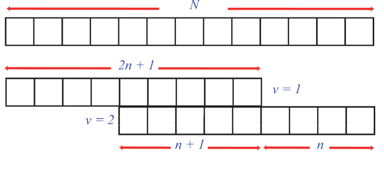
Figure 1: A schematic to clarify how the adaptive detrending method is implemented on desired series.

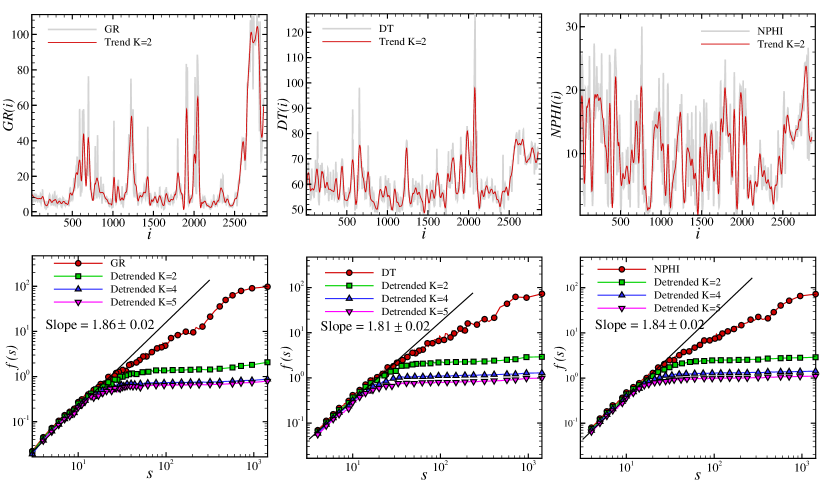
Figure 2: Upper panels show three petrophysical quantities, Gamma ray (GR), sonic transient time (DT) and Neutron porosity (NPHI), respectively, versus depth recorded every $15.4$cm at depth interval $3504.5$m to $3946.8$m for well $\#2$. In these panels the gray line corresponds to original fluctuations while the dark solid line indicates the trend fluctuation constructed by setting $\rm{w}_{adaptive}=101$ and $K=2$ for fitting polynomial in each segment. The lower panels illustrate fluctuation function as a function of scale for different series of well $\#2$. The filled circle symbol shows $f(s)$ for original data set. The filled square symbols are results for clean data by adaptive detrending method with $K=2$. Up-triangle and down-triangle symbols correspond to clean data with $K=4$ and $K=5$, respectively.

V Data description

We use well-log data from four oil wells of Maroon reservoir in southwest of Iran. These data include gamma emission (GR), sonic transient time (DT) and neutron porosity (NPHI) recorded every $15.4cm$. The logged interval contains Asmari region formation, including mainly of fractured carbonate, sand stone, shaly sand and a trace of anhydrate. Gamma log is a criterion for the natural radiation of the composition. Gamma emission is received from shales and shaly sands which have higher radioactivity. Sonic log involves elapsed time for traveling sound wave through a composition. Changing the energy of high energy neutrons during their collision with the component of targets is a benchmark for tracking the existence of hydrogen in the pore space Fedi ; log1 ; log2 . Therefore, NPHI is used for neutron porosity. According to mentioned criteria, the spatial heterogeneity of properties of the large scale porous media, such as porosity, density and the lithology at distinct length scales are determined log3 ; log4 ; log5 . Upper panels of Fig. 2 show GR, DT and NPHI series for well $\#2$ of this region. In these panels the gray line corresponds to original fluctuations while the dark solid line indicates the trend fluctuation constructed by setting $\rm{w}_{adaptive}=101$ and $K=2$ for fitting polynomial in each segment. The lower panels illustrate fluctuation function as a function of scale for different series of well $\#2$. The filled circle symbol shows $f(s)$ for original data set. The filled square symbols is results for clean data by adaptive detrending method with $K=2$. Up-triangle and down-triangle symbols correspond to clean data with $K=4$ and $K=5$, respectively. Obviously, the $f(s)$ for original fluctuations has not unique scaling behavior. This situation gives rise for other sets of data used throughout this paper. Subsequently, one can not determine associated Hurst exponent, then essentially, adaptive detrending or every additional method to remove trend in data must be applied in order to find reliable Hurst exponent. Table 1 contains the Hurst exponent determined by Adaptive-DFA method. Our results confirm that all series belong to the nonstationary process so $H=h-1$. This Hurst exponent is necessary to set up theoretical prediction represented by Eqs. (10) and (24).

$H$	$\#1$	$\#2$	$\#3$	$\#4$
GR	$0.65\pm 0.02$	$0.86\pm 0.02$	$0.84\pm 0.02$	$0.92\pm 0.02$
NPHI	$0.80\pm 0.02$	$0.84\pm 0.02$	$0.76\pm 0.02$	$0.77\pm 0.02$
DT	$0.79\pm 0.02$	$0.81\pm 0.02$	$0.73\pm 0.02$	$0.77\pm 0.02$

Table 1: The Hurst exponent, $H$, of data sets recorded for four wells of the reservoir at $1\sigma$ confidence interval.

$\lambda_{0}^{2}$	$\#1$	$\#2$	$\#3$	$\#4$
GR	$0.042\pm 0.020$	$0.200\pm 0.002$	$0.077\pm 0.003$	$0.040\pm 0.002$
NPHI	$0.023\pm 0.003$	$0.045\pm 0.002$	$0.028\pm 0.002$	$0.029\pm 0.002$
DT	$0.002\pm 0.001$	$0.004\pm 0.001$	$0.004\pm 0.001$	$0.005\pm 0.001$

Table 2: The non-Gaussian parameter, $\lambda_{0}^{2}$ of data sets recorded for four wells of the reservoir at $1\sigma$ confidence interval.

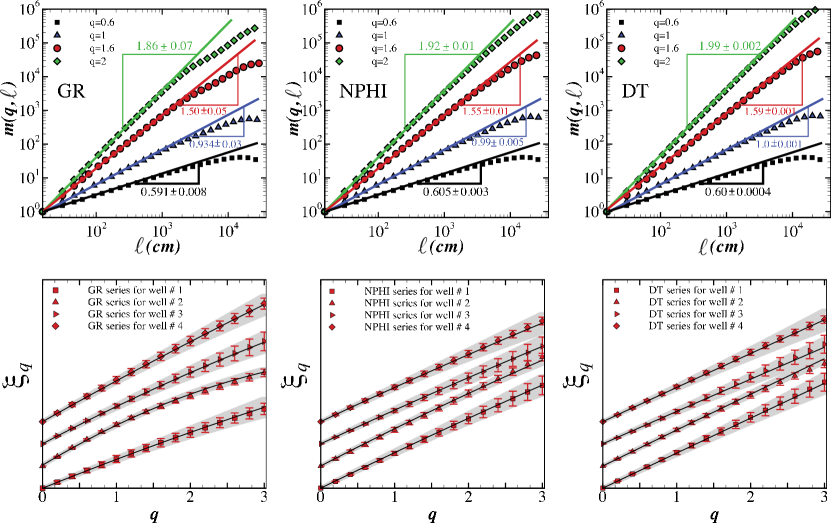
Figure 3: Upper panels show log-log plot of $m(q,\ell)$ versus $\ell$ for $q=0.6$ (square), $q=1$ (triangle), $q=1.6$ (circle) and $q=2$ (diamond) for GR (left panel), NPHI (middle panel) and DT (right panel) for well $\#2$. The lower panels correspond to scaling exponent, $\xi_{q}$, versus $q$ from left to right for GR, NPHI and DT series, respectively for four wells of the reservoir. Symbols correspond to the empirical series and solid lines show theoretical prediction given by Eq. (10) at $1\sigma$ confidence interval corresponding to shaded area. To make more sense we shifted the value of $\xi_{q}$ for different data sets vertically.

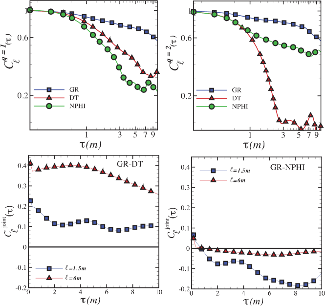
Figure 4: Upper panels indicate increment correlation function $C_{\ell}^{q}(\tau)$ calculated for $q=1$ (left) and $q=2$ (right) versus lag $\tau$ at scale $\ell=1.5m$ (Eq.12). Lower panels illustrate cross-correlation function, $C_{\ell}^{\rm{joint}}(\tau)$, of the petrophysical series for well $\#2$ versus lag $\tau$ at scales $\ell=1.5m$ (square) and $\ell=6.0m$ (delta) for GR-DT (left) and GR-NPHI (right).

VI data analysis

In this article we implement multifractal random walk model to characterize a reservoir by describing some features of petrophysical quantities. As mentioned before, one reliable method for multifractal characteristic of a typical data sets is determined by evaluation of scaling exponent $\xi_{q}$ from the linear state. To this end, Eq. (1) is computed for our data. Upper panels of Fig. 3 indicate log-log plot of $m(q,\ell)$ versus $\ell$ for well $\#2$ at different values of $q$ for various kind of data sets. These plots verify that $m(q,\ell)$ has scaling nature up to a typical characteristic scale (this result is satisfied for all considered wells), consequently, the scaling exponent, $\xi_{q}$ has reliable value at $1\sigma$ confidence interval. The scaling exponent $\xi_{q}$ for the petrophysical quantities has been plotted in the lower panels of Fig. 3. In this plots symbols correspond to numerical results. These results demonstrate that $\xi_{q}$ for all wells is nonlinear for GR and NPHI corresponding to multifractal nature of mentioned quantities. While $\xi_{q}$ is almost linear for DT at all considered wells which argues monofractal behavior. In order to evaluate the theoretical prediction of $\xi_{q}$ (Eq. (10)) and to compare it with that of given by numerical approach, we should determine the corresponding $\lambda_{0}^{2}$ and $H$. The multifractal parameter $\lambda_{0}^{2}$ is the intercept of $\lambda_{\ell}^{2}$ versus $\ell$ determined by Eq. (6) koohi . The Hurst exponent ,$H$, of the data sets has been estimated by adaptive-DFA peng94 ; Hu ; bunde02 . The value of Hurst exponent and multifractal parameter for GR, DT and NPHI have been reported in Tables. 1 and 2. From statistical point of view, according to Hurst exponent, one can not discriminate GR, NPHI and DT from each other, while the value of $\lambda_{0}^{2}$ can, namely $\lambda_{0}^{2}({\rm GR})>\lambda_{0}^{2}({\rm NPHI})\gg\lambda_{0}^{2}({\rm DT})$.

Plugging $H$ and $\lambda_{0}^{2}$ of each data in Eq. (10), theoretical value of $\xi^{\rm The}_{q}$ is obtained. Solid lines in the lower panels of Fig. 3 correspond to $\xi^{\rm The}_{q}$. Our results are consistent with that of given directly from Eq. (1) at $1\sigma$ confidence interval. To make more sense, we shifted the value of $\xi_{q}$ for different data sets vertically. The multifractal property of GR for four considered wells expresses that various values of fluctuations in GR series don’t exhibit a global scaling behavior. This means that fractal nature of Gamma ray series in the reservoir is a local property from the value of fluctuations point of view. Since DT series is based on the propagation of sound wave through the media, it follows the continuum regions as much as possible. Subsequently, the multifractality would be suppressed. Meanwhile, NPHI data set, has less multifractality nature than GR series. It represents inhomogeneity distribution of Hydrogen in the pores. As mentioned in section II, the larger value of $\lambda_{0}^{2}$, the fatter non-Gaussian tail of PDF resulting in multifractal behavior. Namely, in such case, the source of multifractality is large scale fluctuations corresponding to rare events. Dependency of multifractal behavior to length scale, $\ell$, is determined by the shape of PDF. Koohi et al. koohi have shown that for mentioned data sets of well $\#2$, non-Gaussianity is scale invariant for GR and DT, while $\lambda_{\ell}^{2}$ decreases by increasing $\ell$. According to current analysis based on $\xi_{q}$, one can find a consistency between previous and present results. Indeed, GR is strongly multifractal and the value of associated $\lambda_{\ell}^{2}$ has considerable value. However, the value of $\lambda_{\ell}^{2}$ for DT is constant versus $\ell$, but the individual value is small in comparison to GR’s. Our approach enables us to answer the question concerning the nature of multifractality. According to the shape of PDF modeled by Eq. (6) and the comportment of $\lambda_{\ell}^{2}$ as a function of $\ell$ koohi , we find that multifractal feature is caused by the long-range correlations in mentioned series.

In order to investigate the effect of correlations in petrophysical quantities, the correlation function for $q=1$, and $q=2$, are calculated by means of Eq. (12). Upper panels of Fig. 4 shows the correlation function of the first and second increment moments of the data sets for well $\#2$. The long-range correlation function for GR reveals the global strong correlations in shaly layers of the reservoir. While, the rapid suppression of correlation function for second moment of increment for DT demonstrates that this data set belongs to almost monofractal category which is consistent with our pervious results regarding $\xi_{q}$. In addition, the considerable value of correlation function for large fluctuations of NPHI demonstrates that this quantity is non-Gaussian and multifractal at small scales. The same results have been confirmed for other wells.

The petrophysical quantities have mutual correlations in the reservoir. The non-Gaussian PDF of GR at all scales reveals that GR is playing as a background role in the system that affects other relevant quantities koohi . Additional investigation in the context of multiplicative cascades multifractal formalism is satisfied by cross-correlation of stochastic variances as Kiy06 :

$$C_{\ell}^{\rm joint}(\tau)\equiv\left\langle\left[\bar{\omega}^{(\ell)}_{1}(i+\tau)-\langle\bar{\omega}^{(\ell)}_{1}\rangle\right]\left[\bar{\omega}^{(\ell)}_{2}(i)-\langle\bar{\omega}^{(\ell)}_{2}\rangle\right]\right\rangle$$ (31)

with

$$\bar{\omega}^{(\ell)}_{\diamond}(i) = \frac{1}{2}\ln\sigma^{2}_{\diamond}(\ell;i)$$ (32)

$$\sigma^{2}_{\diamond}(\ell;i) = \frac{1}{\ell}\sum_{j=1+(i-1)\ell}^{i\ell}\delta_{\ell}x^{2}_{\diamond}(j)$$ (33)

where $(\diamond)$ is replaced by $(1)$ and $(2)$ for first and second data sets in the underlying pair. To explore the nature of cross-correlation for series we compute $C_{\ell}^{\rm joint}(\tau)$ for GR-NPHI and GR-DT pairs associated to well $\#2$. Fig. 4 indicate the cross-correlations at scale $\ell$ as a function of $\tau$. For GR-DT pair, cross-correlation has positive sign and behaves as long-range phenomenon for $\ell=1.5$m and $\ell=6.0$m. For GR-NPHI, there is an anti-correlated behavior and by increasing $\ell$, the magnitude of mutual interaction asymptotically goes to zero. Positive cross-correlation for GR-DT probably corresponds to existence of continuum shaly region in which sonic sound prefers to pass it, therefore fluctuations in this pair are synchronized resulting in possessing positive cross-correlation based on stochastic variance. However, the negative cross-correlation for GR-NPHI pair implies the fact that regions with shaly layers prevent gathering of Hydrocarbon or water in the pores. To make more sense and to quantify the joint multifractality, we rely on approach explained in section III, and determine the value of joint multifractal parameter, $L_{0}$ Muzy2 . The values of $L_{0}$ for GR-DT and GR-NPHI at $1\sigma$ confidence interval for four considered wells in the reservoir are reported in Table 3. These values demonstrate that the nature of joint multifractality is related to magnitude of cross-correlation and they are compatible with previous interpretations. Using Eq. (23), the slope of log-log plot of $m_{\rm joint}(q_{1},q_{2};\ell)$ versus $\ell$ for $q_{1}=q_{2}$ gives $\xi_{q}^{\rm joint}$. Upper panels of Fig. 5 illustrate the log-log plot of $m_{\rm joint}(q,\ell)$ versus $\ell$ for pairs of GR-DT and GR NPHI for well $\#2$. Lower panels of Fig. 5 correspond to the numerical and theoretical values of $\xi_{q}^{\rm joint}$ for mentioned pairs and for four wells of the reservoir. In order to estimate the theoretical prediction of $\xi_{q}^{\rm joint}$, we use Eq. (24) and take into account the relevant values of $\xi_{q}$ and $L_{0}$. The solid lines in the lower panels of Fig. 5 correspond to this approach and shaded area indicates the $68\%$ confidence interval. Joint multifractality is positive for GR-DT causing the convex shape for $\xi_{q}^{\rm joint}$, while the negative value of $L_{0}$ reduces this convexity in $\xi_{q}^{\rm joint}$ for GR-NPHI.

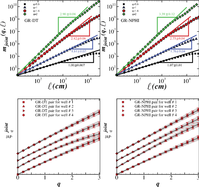
Figure 5: The upper panels show log-log plot of joint moment $m_{\rm{joint}}(q,\ell)$ with $q_{1}=q_{2}=q$ versus $\ell$ for $q=0.6$ (square), $q=1$ (triangle), $q=1.6$ (circle) and $q=2$ (diamond) for GR-DT pair (upper left) and GR-NPHI pair (upper right) for well $\#2$. The lower panels indicate joint scaling exponent, $\xi_{q}^{\rm{joint}}$, versus $q$ for GR-DT (left) and GR-NPHI (right) for four wells of reservoir. The symbols correspond to numerical approach and solid lines represent theoretical formula given by Eq. (24) for $68\%$ confidence interval according to shaded area. To make more sense, we shifted the value of $\xi_{q}^{\rm joint}$ for different data sets vertically.

$L_{0}$	$\#1$	$\#2$	$\#3$	$\#4$
GR-NPHI	$-0.004\pm 0.010$	$-0.068\pm 0.002$	$-0.032\pm 0.001$	$-0.015\pm 0.001$
GR-DT	$0.003\pm 0.010$	$0.062\pm 0.001$	$0.021\pm 0.001$	$0.016\pm 0.002$

Table 3: The joint multifractal parameter, $L_{0}$ of data sets for four wells of the reservoir at $1\sigma$ confidence interval.

VII Summary and Conclusion

In this paper, we relied on multifractal random walk and joint-multifractal random walk approaches to analyze some features of petrophysical quantities represented by GR, NPHI and DT as some of petroleum reservoir indicators. Mentioned data sets have been collected in well-logging through four wells in Maroon reservoir in southwest of Iran.

To infer statistical information through statistical indicators, one must take care about following strategy: when there are more than a few indicators existing in a typical phenomenon, it is important to estimate how efficient they are and how they are cross-correlated. To this end, we should determine the degree of correlation between mentioned indicators. In other words, if the indicators are cross-correlated to each other, probably, the content of their information is less than two completely independent indicators. To analyze oil wells, lots of indicators have been introduced and without having knowledge about their cross-correlations, results coming from each indicators are not reliable. In the oil wells, as we get closer to oil reservoir, the properties of the medium changes. The effect of this variation causes a non-Gaussian behavior of indicators, hence joint multifractal random walk could be a useful measure to examine this kind of cross-correlation between these indicators. multifractal random walk model has been introduced according to the concept of multiplicative random cascades in multifractal formalismBacry ; Muzy1 . The parameter which controls the strength of multifractality is $\lambda_{0}^{2}$. The larger value of $\lambda_{0}^{2}$, the higher probability of finding large scale fluctuations in a system causing a non-Gaussian PDF and strong multifractality. This gives rise to non-linear scaling exponent of absolute moment of fluctuations, $\xi_{q}$, (Eq. (1)) versus $q$. In order to explore the mutual effects, joint multifractal random walk of data sets have been considered under the notion of joint multiplicative cascade processes. The cross-correlation in the fluctuations of stochastic variances causes the joint multifractality represented by joint multifractal parameter, $L_{0}$. According to the multiplicative approach, there is a relation between $\xi_{q}$ and $\lambda_{0}^{2}$ which allows us to check the consistency of both approaches (Eq. (10)). In addition, for joint analysis, theoretical prediction for $\xi_{q}^{\rm joint}$ using the value of $H$, $\lambda_{0}^{2}$ and $L_{0}$ exponents can be written according to Eq. (24). The positive or negative value of $L_{0}$ is due to the existence of persistent or anti-persistent correlation of large fluctuations of two underlying series. The positive value of $L_{0}$ causes the convex shape of $\xi^{\rm joint}_{q}$, however, the negative value of $L_{0}$ decreases the convexity of $\xi^{\rm joint}_{q}$.

Our results demonstrated that GR in Maroon reservoir exhibits strong multifractality due to the almost high value of $\lambda_{0}^{2}$, consequently $\xi_{q}$ is non-linear (see Fig. 3). Also its PDF is non-Gaussian and scale-invariant koohi . This demonstrates high probability of the occurrence of large fluctuations in GR series which emitted from shaly layers and leads to multifractal property. While the value of $\lambda_{0}^{2}$ for DT can be ignored (Table 3). This gives rise to a linear function for $\xi_{q}$ which is a hallmark of monofractal behavior. This phenomenon is explained based on the fact that sound wave follows the continuum regions in the reservoir, hence this quantity exhibits monofractal property. For NPHI data set, since the shape of PDF is scale dependent koohi and its $\lambda_{0}^{2}$ is less than GR’s, our analysis indicated $\xi_{q}$ is non-linear. Indeed, inhomogeneity distribution of Hydrogen in the pores at small scales results in multifractal behavior of NPHI only at small scales.

Joint analysis of data sets for all mentioned wells of Maroon reservoir proved the negative and positive values of $L_{0}$ for GR-NPHI and GR-DT pairs, respectively. Computational value of joint moments, $\xi_{q}^{\rm joint}$ displayed that joint multifractality for GR-DT is almost larger than GR-NPHI pair (Fig. 5). Lower panels of Fig. 5 proved that the numerical and theoretical prediction for $\xi_{q}^{\rm joint}$ are in agreement at $1\sigma$ confidence interval. From petrophysical point of view, one can mention that sonic sound prefers to pass through the continuum shaly region, so we expect the positive cross-correlation between GR-DT pair corresponding to statistical synchronization of fluctuations of mentioned pair, $L_{0}>0$. In addition, in the presence of shaly layers the probability of finding pores in media decreases, subsequently we expect negative cross correlation between GR and NPHI indicators corresponding to $L_{0}<0$. Finally, it could be interesting to apply these methods to asses other indicators and available data of other reservoirs to examine other effects.

Acknowledgments: Authors are grateful to H. Dashtian for preparing data used in this research. S.M.S.M. is tankful to Associate office of ICTP.

VIII APPENDIX

In this appendix by relying on multivariate form of PDF, we show a proof in details for the relations, given in Eqs.(24) and (25). Suppose an stochastic increment for a bivariate process $\textbf{x}(t)$ with lag $\ell$ as:

$$\delta_{\ell}\mathbf{x}(t) \equiv \delta_{\ell}x_{1}(t)\delta_{\ell}x_{2}(t)$$ (34)

$$= \left[x_{1}(t+\ell)-x_{1}(t)\right]\left[x_{2}(t+\ell)-x_{2}(t)\right]$$

For convenience, we denote the processes $x_{1}(t)$ and $x_{2}(t)$ by $x_{1}$ and $x_{2}$, respectively. The joint moment of the processes reads as:

$$m(q_{1},q_{2},\ell)\equiv\langle|\delta_{\ell}x_{1}|^{q_{1}}|\delta_{\ell}x_{2}|^{q_{2}}\rangle$$

$$= \int|\delta_{\ell}x_{1}|^{q_{1}}|\delta_{\ell}x_{2}|^{q_{2}}P_{\ell}\left(\delta_{\ell}x_{1},\delta_{\ell}x_{2}\right)d(\delta_{\ell}x_{1})d(\delta_{\ell}x_{2})$$

where $P_{\ell}\left(\delta_{\ell}x_{1},\delta_{\ell}x_{2}\right)$ is equivalent to Eq. (20) and can be defined as follows:

$$P_{\ell}(\delta_{\ell}x_{1},\delta_{\ell}x_{2}) = \int\int G_{\ell,\beta\times\ell}(u_{1},u_{2})e^{-(u_{1}+u_{2})}$$

$$P_{\beta\times\ell}(e^{-u_{1}}\delta_{\ell}x_{1},e^{-u_{1}}\delta_{\ell}x_{2})du_{1}du_{2}$$

$\delta_{\ell}x_{1}$ and $\delta_{\ell}x_{2}$ have scaling behavior:

$$\delta_{\ell}x_{1}=\ell^{H_{1}}\delta x_{1}\ \ \ \ ,\ \ \ \ \delta_{\ell}x_{2}=\ell^{H_{2}}\delta x_{2}$$ (37)

Plugging Eqs.(VIII) and (37) in Eq. (VIII) then, by changing the variables:

$$x^{\prime}_{1}\equiv e^{-u_{1}}\delta x_{1}\ \ \ \ ,\ \ \ \ x^{\prime}_{2}\equiv e^{-u_{1}}\delta x_{2}$$ (38)

the joint moment, Eq. (VIII), becomes:

$$m(q_{1},q_{2},\ell)=\ell^{q_{1}H_{1}}\ell^{q_{2}H_{2}}\left(\int\int(x^{\prime}_{1})^{q_{1}}(x^{\prime}_{2})^{q_{2}}P(x^{\prime}_{1},x^{\prime}_{2})dx^{\prime}_{1}dx^{\prime}_{2}\right)\left(\int\int e^{q_{1}u_{1}}e^{q_{2}u_{2}}G_{\ell}(u_{1},u_{2})du_{1}du_{2}\right)$$ (39)

The first double integral in the above equation introduces the prefactor:

$$\mathcal{A}_{q_{1},q_{2}}=\int\int(x^{\prime}_{1})^{q_{1}}(x^{\prime}_{2})^{q_{2}}P(x^{\prime}_{1},x^{\prime}_{2})dx^{\prime}_{1}dx^{\prime}_{2}$$ (40)

where $P(x^{\prime}_{1},x^{\prime}_{2})$ is a joint Gaussian PDF:

$$P(x^{\prime}_{1},x^{\prime}_{2})=\frac{1}{2\pi\sqrt{\rm{Det}(\mathbf{\Sigma}_{(\ell)})}}\ \exp\left({-\frac{\mathbf{x^{\prime}}^{T}\cdot\mathbf{\Sigma}_{(\ell)}^{-1}\cdot\mathbf{x^{\prime}}}{2}}\right)$$ (41)

with covariance matrix, $\mathbf{\Sigma}_{(\ell)}$ represented by:

$$\mathbf{\Sigma}_{(\ell)}\equiv\left(\begin{array}[]{cc}\Sigma_{(\ell)}^{11}&\Sigma_{(\ell)}^{12}\\ \Sigma_{(\ell)}^{21}&\Sigma_{(\ell)}^{22}\\ \end{array}\right)$$ (42)

The prefactor $\mathcal{A}_{q_{1},q_{2}}$ can be written as two separated integrals:

$$\mathcal{A}_{q_{1},q_{2}} = \frac{1}{2\pi\sqrt{(1-S_{\ell}^{2})}}\int(x^{\prime}_{1})^{q_{1}}e^{-\frac{(x^{\prime}_{1})^{2}}{2(1-S_{\ell}^{2})}}dx^{\prime}_{1}$$ (43)

$$\int(x^{\prime}_{2})^{q_{2}}e^{-\frac{(x^{\prime}_{2})^{2}}{2(1-S_{\ell}^{2})}}dx^{\prime}_{2}$$

where covariance coefficient, $S_{\ell}$, is defined as $S_{\ell}=\frac{\Sigma_{(\ell)}^{12}}{\sigma_{1}(\ell)\sigma_{2}(\ell)}$. In order to calculate the second integral in Eq. (39), Fourier transformation of $G_{\ell}(u_{1},u_{2})$ is implemented which is defined as:

$$G_{\ell}(k_{1},k_{2})=e^{\ln\ell(i\mathbf{k}^{T}\Gamma-\frac{1}{2}\mathbf{k}^{T}.\Lambda.\mathbf{k})}$$ (44)

where $\Gamma$ is bivariate mean vector, $\Gamma=(\Gamma_{1},\Gamma_{2})$. Thus, the second integral determining the scaling dependence of the joint moment is estimated as:

$$\int\int e^{q_{1}u_{1}}e^{q_{2}u_{2}}G_{\ell}(u_{1},u_{2})du_{1}du_{2}={\ell}^{q_{1}\Gamma_{1}+q_{2}\Gamma_{2}-\frac{1}{2}\left(\lambda_{1}^{2}q_{1}^{2}+\lambda_{2}^{2}q_{2}^{2}\right)-q_{1}q_{2}L_{0}}$$ (45)

In order to obtain the mean values of $\Gamma_{1}$ and $\Gamma_{2}$, we assume the compact support case for which in absence of cross correlation ($L_{0}=0$) the scaling exponent of multifractal portion vanishes for $q_{1}=q_{2}=1$. This yields $\Gamma_{1}=\frac{\lambda_{1}^{2}}{2}$ and $\Gamma_{2}=\frac{\lambda_{2}^{2}}{2}$, thus the joint moment becomes:

$$m(q_{1},q_{2},\ell)=\mathcal{A}_{q_{1},q_{2}}\ell^{\xi_{q_{1}}^{(1)}+\xi_{q_{2}}^{(2)}-q_{1}q_{2}L_{0}}$$ (46)

where $\xi_{q_{i}}^{(i)}=q_{i}H_{i}-\frac{\lambda_{i}^{2}}{2}q_{i}(q_{i}-1)$ with $i=1,2$ is the scaling exponent of each single process.

References

- (1) M. Lazǎr and C. Lazǎr , Analizǎ Statistico - Economicǎ, Economic Publishing House, Bucharest, (2012), p. 25
- (2) Mohammed Abdul Rasheed , Mutnuri Lakshmi, Deshoju Srinu and Anurodh Mohan Dayal, Pet.Sci. (2011) 8:264-268.
- (3) D.V. Ellis, (1987). Well Logging for Earth Scientists. New York City: Elsevier Science Publishing.
- (4) P.P. Theys, (1999), Log Data Acquisition and Quality Control, second edition, Paris, France: Editions Technip
- (5) J.R. Hearst, P.H. Nelson and F.L. Paillet, (2000). Well Logging for Physical Properties, second edition. New York City: John Wiley & Sons.
- (6) E. Bacry, J. Delour, J. F. Muzzy, Phys. Rev. E 64 (2001) 026103.
- (7) J.-F. Muzy, J. Delour and E. Bacry, Eur. Phys. J. B 17 (2000) 537.
- (8) E.Bacry, J. Delour, J.F. Muzy, arXiv:cond-mat/0009260 A multivariate multifractal model for return fluctuations.
- (9) J. F. Muzy, D. Sornette, J. Delour, A. Arneodo, Quantitative Finance, 1 (2001) 131.
- (10) S. Ghashghaie, W. Breymann, J. Peinke, P. Talkner, Y. Dodge, Nature (London) 381 (1996) 767.
- (11) K. Kiyono, Z. R. Struzik, Y. Yamamoto, Phys. Rev. Lett. 96 (2006) 068701.
- (12) G. R. Jafari, M. Sadegh Movahed, P. Noroozzadeh, A. Bahraminasab, M. Sahimi, F. Ghasemi, M. Reza Rahimi Tabar, International Journal of Modern Physics C 18 (2007) 1689.
- (13) K. Kiyono, Z. R. Struzik, N. Aoyagi, S. Sakata, J. Hayano, Y. Yamamoto, Phys. Rev. Lett. 93 (2004) 178103; K. Kiyono, Z. R. Struzik, N. Aoyagi, F. Togo, Y. Yamamoto, Phys. Rev. Lett. 95 (2005) 058101.
- (14) P. Manshour, S. Saberi, M. Sahimi, J. Peinke, A. F. Pacheco, M. R. RahimiTabar, Phys. Rev. Lett. 102 (2009) 014101.
- (15) Lciano Telesca, Ashutosh Chamoli, Michele Lovallo, Tony Alfredo Stabile, Pure and Applied Geophysics 10.1007/s00024-014-0862-3 (2014)
- (16) S. K. Aggarwal, M. Lovallo, P. P. Khan, B. K. Rastogi, L. Telesca, Physica A 426, 56-62 (2015)
- (17) F. Shayeganfar, S. Jabbari-Farouji, M. S. Movahed, G.R. Jafari, M. R. Tabar, Phys. Rev. E 81 (2010) 061404.
- (18) T. Vicsek, Fractal Growth Phenomena (World Scientific, Singapore, 1989)
- (19) A. L. Barabsi and H. E. Stanley, Fractal Concepts in Surface Growth (Cambridge University Press, Cambridge, 1995)
- (20) L. Sorriso-Valvo, V. Carbone, P. Veltri, G. Consolini, R. Bruno, Geophys. Res. Lett. 26 (1999) 1801.
- (21) Luciano Telesca, Michele Lovallo, J. Stat. Mech. P07001 (2011).
- (22) M. Sadegh Movahed, G. R. Jafari, F Ghasemi, Sohrab Rahvar, and M Reza Rahimi Tabar, J. Stat. Mech. doi:10.1088/1742-5468/2006/02/P02003
- (23) Zu-Guo Yu, V. Anh, R. Eastes, J. Geophysical Research,114 (2009) A05214.
- (24) S. Hajian and M. Sadegh Movahed, Physica A 389 (2010) 4942
- (25) Kantelhardt, J. W., E. Koscielny-Bunde, D. Rybski, P. Braun, A. Bunde, and S. Havlin, JOURNAL OF GEOPHYSICAL RESEARCH, VOL. 111, D01106, doi:10.1029/2005JD005881 (2006).
- (26) S. M. S. Movahed and Evalds Hermanis, Physica A 387, 915 (2008).
- (27) U. Frisch, Turbulence, Cambridge University Press, Cambridge (1995).
- (28) C. Meneveau and K. R. Sreenivasan, Phys. Rev. Lett. 59 (1987) 1424; A. Arneodo, J.-F. Muzy, D. Sornette, Eur. Phys. J. B 2 (1998) 277; E. Bacry, J. Delour, J.F. Muzy, Physica A 299 (2001) 84 ; Gao-Feng Gu, Wei-Xing Zhou, Phys. Rev. E 74 (2006) 061104;S. Hosseinabadi, M. A. Rajabpour, M. Sadegh Movahed, S. M. Vaez Allaei, Phys. Rev. E 85 (2012) 031113.
- (29) T. C. Halsey et al., Phys. Rev. A 33 (1986) 1141.
- (30) G. Paladin and A. Vulpiani, Phys. Rep. 156 (1987) 147.
- (31) C. Meneveau and K. R. Sreenivasan, J. Fluid Mech. 224 (1991) 429.
- (32) Z. Koohi Lai, G.R. Jafari, Physica A, 392 (2013) 5132.
- (33) A. Naert, L. Puech, B. Chabaud, J. Peinke, B. Cataing and B. Hbral, J. Phys. II (France) 4 (1994) 215.
- (34) B. Chabaud, A. Naert, J. Peinke, F. Chill , B. Cataing and B. Hbral, Phys. Rev. L., 73 (1994) 3227.
- (35) E. A. Novikov, Phys. Fluids A 2 (1990) 814; Phys. Rev. E 50 (1994) R3303.
- (36) F. E. A. Leite, Ral Montagne, G. Corso, G. L. Vasconcelos, L. S. Lucena, PhysicaA 387 (2008) 1439.
- (37) Ral Montagne, Giovani L. Vasconcelos, PhysicaA 371 (2006) 122.
- (38) M. Christie, V. Demyanov, D. Erbas, J. Comput. Phys. 217 (2006) 143.
- (39) Z. Koohi Lai, S. Vasheghani Farahani, G.R. Jafari, Physica A, 391 (2012) 5076.
- (40) M. Fedi, D. Fiore, M. La Manna, Regularity analysis Applied to well (2005).
- (41) J. L. Jensen, L. W. Lake, P. W. M. Corbett, D. J. Goggin, Statistics for Petroleum Engineers and Geoscientists, 2nd ed., Prentice Hall, New Jersey, (2000).
- (42) M. Sahimi, Flow and Transport in Porous Media and Fractured Rock, 2nd ed., Wiley-VCH, Berlin, (2011).
- (43) J. Feder Fractals, (1988).
- (44) J. Gao, Y. Cao, W. W. Tung, J. Hu, Multiscale analysis of complex time series John Wiley and Sons (2007).
- (45) R. Benzi, S. Ciliberto, R. Tripiccione, C. Baudet, F. Massaioli, S. Succi, Phys. Rev. E. 48 (1993) R29.
- (46) B. Castaing, Y. Gagne, E. J. Hopfinger, Physica D 46 (1990) 177.
- (47) U. Frisch and D. Sornette, J. Phys. I (France) 7 (1997) 1155.
- (48) B. B. Mandelbrot, J. Fluid. Mech 62 (1974) 331.
- (49) J. P. Kahane, J. Peyriere, Adv. Math 22 (1976) 131.
- (50) H. G. E. Hentschel, Phys. Rev. E. 50 (1994) 243.
- (51) A. Arneodo, J. F. Muzy, S. Roux, J. Phys. France 7 (1997) 363.
- (52) K. Kiyono, Z. R. Struzik, Y. Yamamoto, Phys. Rev. E. 76 (2007) 041113.
- (53) F. Shayeganfar, S. Jabbari-Farouji, M. Sadegh Movahed, G. R. Jafari, M. Reza Hahimi Tabar, Phys. Rev. E. 80 (2009) 061126.
- (54) B. Podobnik and H. Euge Stanley, Phys. Rev. Lett. 100 (2008) 084102.
- (55) Wei-Xing Zhou, Phys. Rev. E 77 (2008) 066211.
- (56) C.-K. Peng, S.V. Buldyrev, A.L. Goldberger, S. Havlin, F. Sciortino, M. Si- mons, and H.E. Stanley, Nature, 356, 168-170 (1992).
- (57) C.-K. Peng, S. V. Buldyrev, S. Havlin, M. Simons, H. E. Stanley, and A. L. Goldberger, Phys. Rev. E 49, 1685-1689 (1994).
- (58) Ying-Hui Shao, Gao-Feng Gu, Zhi-Qiang Jiang, Wei-Xing Zhou & Didier Sornette, Scientific Reports 2, 835 (2012).
- (59) Jing Hu, Jianbo Gao and Xingsong Wang, JSTAT, P02066 (2009).
- (60) Yu Zhou and Yee Leung, J. Stat. Mech. (2010) P12006.
- (61) S. V. Buldyrev, A. L. Goldberger, S. Havlin, R. N. Mantegna, M. E. Matsa, C.-K. Peng, M. Simons, and H. E. Stanley, Phys. Rev. E 51, 5084 (1995).
- (62) J. W. kantelhardt, S. A. Zschiegner, E. Koscielny-Bunde, A. Bunde, S. Havlin and H. E. Stanley, Physica A 316, 87 (2002).
- (63) A. Bunde, S. Havlin, J. W. Kantelhardt, T. Penzel, J. H. Peter and K. Voigt, Phys. Rev. Lett. 85, 3736 (2000).
- (64) M. S. Taqqu, V. Teverovsky, and W. Willinger, Fractals 3, 785 (1995).
- (65) G. Reza Jafari, Muhammad Sahimi, M. Reza Rahimi Tabar, M. Reza Rasaei, Phys. Rev. E 83 (2011) 026309.
- (66) R. B. Ferreira, V. M. Vieira, Iram Gleria, M. L. Lyra , Physica A 388 (2009) 747.
- (67) M. Sahimi, S. E. Tajer, Phys. Rev. E 71 (2005) 046301.
- (68) K. Hu, P. C. Ivanov, Z. Chen, P. Carpena, H. E. Stanley, Phys. Rev. E. 64 (2001) 011114.