Dynamics of extended bodies in a Kerr spacetime with spin-induced quadrupole tensor

Abstract

The features of equatorial motion of an extended body in Kerr spacetime are investigated in the framework of the Mathisson-Papapetrou-Dixon model. The body is assumed to stay at quasi-equilibrium and respond instantly to external perturbations. Besides the mass, it is completely determined by its spin, the multipolar expansion being truncated at the quadrupole order, with a spin-induced quadrupole tensor. The study of the radial effective potential allows to analytically determine the ISCO shift due to spin and the associated frequency of the last circular orbit.

I Introduction

The description of the gravitational interaction between the constituents of a binary system in the general theory of relativity requires taking into due account their internal structure. The orbital dynamics of two bound compact objects is tackled in the literature by a plenty of different methods resorting to various approximation schemes. Analytic approaches include notably the post-Newtonian approximation Blanchet (2014), possibly implemented using effective field theory techniques Goldberger (2007), as well as the gravitational self-force corrections to geodesic motion Poisson et al. (2011), which can both be combined efficiently by means of the “effective-one-body” approach Buonanno and Damour (1999); Damour (2014).

When the mass of one body is much smaller than the other, the problem boils down to studying the dynamics of an extended body in a fixed background field, generated by the heavier mass. In this approximation, a self-consistent model describing the evolution of both linear and angular momenta for pole-dipole sources was developed by Mathisson Mathisson (1937), Papapetrou Papapetrou (1951); Corinaldesi and Papapetrou (1951), Pirani Pirani (2009), Tulczyjew Tulczyjew (1959), and later generalized to bodies endowed with higher multipoles by Dixon Dixon (1964, 1970a, 1970b, 1973, 1974). The Mathisson-Papapetrou-Dixon (MPD) model accounts for the motion, on a fixed background, of a point-size test object with internal degrees of freedom, in the absence of significant gravitational back reaction.

The main astrophysical situation for which a full relativistic treatment is needed occurs when the object — assumed to be compact to avoid tidal disruption — experiences the strong field produced by a nearby black hole. In that case, the MPD approach may be used to investigate the evolution of the system, but the parameters of the model must be regarded as effective ones Harte (2012). Although self-force effects are not negligible on larger-than-orbital time scales, they only yield higher-order corrections. On the other hand, combined with dimensional regularization, the MPD model is appropriate to describe the dynamics of (self-gravitating) compact binaries including finite-size effects, in the post-Newtonian framework Owen et al. (1998); Faye et al. (2006); Bohé et al. (2015). It yields results that are dynamically equivalent to those derived from suitable effective actions Porto (2006); Porto and Rothstein (2006); Barausse et al. (2009). The “skeleton” stress-energy tensor encoding the MPD evolution is known at the quadrupolar level Steinhoff and Puetzfeld (2010). Its octupolar contributions have also been obtained recently Marsat (2015) assuming an effective, Bailey & Israel type, Lagrangian Bailey and Israel (1975). Those corresponding explicit expressions have been used to build accurate theoretical templates for the signal of gravitational radiation emitted by those sources Marsat et al. (2014); Bohé et al. (2015); Marsat (2015); Buonanno et al. (2013), in the context of the data analysis of gravitational-wave observatories, such as the advanced Virgo vir and LIGO lig detectors, the future cryogenic interferometer KAGRA kag or, possibly, the space-based observatory eLISA eLISA Consortium (2013), a candidate for the future L3 mission of the European Space Agency. Most of post-Newtonian expressions can be checked by comparing them to the test-body counterparts, in the extreme mass-ratio limit.

In this paper we study the dynamics of an extended body endowed with both spin and quadrupole moment in a Kerr spacetime using the MPD model. The motion is assumed to be confined on the equatorial plane, the spin vector of the body being aligned with the axis of rotation of the central object. In previous works, we have discussed the effects on the dynamics of a general quadrupole tensor in both Schwarzschild and Kerr spacetimes Bini and Geralico (2013, 2014a, 2014b). Here, we consider more specifically the case of a spin-induced quadrupole tensor. We assume that the object reaches thermodynamic equilibrium in its proper frame on time scales that are very short compared with the orbital period and neglect the tidal deformations. Its internal state thus depends adiabatically on the mass and the (instantaneous) spin. Using effective field theory arguments, it is then straightforward to check that the body quadrupole is actually quadratic in the spin. This situation was described in details by Steinhoff & Puetzfeld Steinhoff and Puetzfeld (2012), who developed a very general framework to include quadratic in spin corrections as well as tidal interactions in the MPD scheme, with special attention to the study of the binding energy of the system as obtained from the analysis of the associated effective potential. Later, Hinderer et al. Hinderer et al. (2013) performed an analysis of the corresponding dynamics, in order to compare the periastron advance and precession frequencies with those of a different approach, but restricted themselves to a very special (although physically motivated) choice of the quadrupole tensor, leading to great simplifications in the analytic treatment.

Here, we shall assume the same form of the quadrupole tensor as in Ref. Steinhoff and Puetzfeld (2012), but neglect quadrupolar tides, i.e., our quadrupole tensor is of the electric-type only and is proportional to the trace-free part of the square of the spin tensor by a constant parameter, whose numerical value is a property of the body under consideration. For neutron stars such a quantity depends on the equation of state Laarakkers and Poisson (1999), while it is exactly 1 for black holes. We keep it a free parameter of the model that can affect associated observables, like the energy and the angular momentum, which we computed explicitly and compared with the results of Ref. Hinderer et al. (2013), or the Innermost Stable Circular Orbit (ISCO) and its frequency, discussed here in details. We achieve a fully analytic treatment of the MPD equations in a “perturbative” scheme, obtaining corrections to geodesic motion up to the second order in spin.

Throughout this work we use geometrical units, setting the Newton constant $G$ and the speed of light $c$ to 1. Tensors are represented either in abstract notation or in index notation combined with the Einstein convention, depending on the context. Greek indices refer to spacetime coordinates and vary from 0 to 3, i.e., $\mu=0,1,2,3$, whereas Latin indices, ranging from 1 to 3, label space coordinates. The notation $\partial_{\mu}$ stands indifferently for the partial derivative with respect to the $\mu$th coordinate $x^{\mu}$ or for the coordinate basis vector associated to $x^{\mu}$, while ${\rm d}$ denotes the exterior derivative. The spacetime metric $g_{\mu\nu}$, taken to have signature $(-,+,+,+)$, defines a unique Levi-Civita covariant derivative, $\nabla_{\mu}$ and an associated Riemann curvature $R^{\mu}{}_{\nu\alpha\beta}$, with the convention that $R^{\mu}{}_{\nu\alpha\beta}v^{\nu}=(\nabla_{\alpha}\nabla_{\beta}-\nabla_{\beta}\nabla_{\alpha})v^{\mu}$ for any vector field $v^{\mu}$. Symmetrization of a tensor $T$ over a set indices is indicated by round brackets enclosing them: $T^{(\mu\nu)}=(T^{\mu\nu}+T^{\nu\mu})/2$. Instead, for index antisymmetrization, square brackets are used: $T^{[\mu\nu]}=(T^{\mu\nu}-T^{\nu\mu})/2$.

II MPD description of extended bodies

In the quadrupole approximation, the MPD equations read

$$\frac{{\rm D}P^{\mu}}{{\rm d}\tau} =-\frac{1}{2}\,R^{\mu}{}_{\nu\alpha\beta}\,U^{\nu}\,S^{\alpha\beta}-\frac{1}{6}\,\,J^{\alpha\beta\gamma\delta}\,\nabla^{\mu}R_{\alpha\beta\gamma\delta}$$

$$\equiv F^{\mu}_{\rm(spin)}+F^{\mu}_{\rm(quad)}\,,$$ (1)

$$\frac{{\rm D}S^{\mu\nu}}{{\rm d}\tau} =2\,P^{[\mu}U^{\nu]}+\frac{4}{3}\,J^{\alpha\beta\gamma[\mu}R^{\nu]}{}_{\gamma\alpha\beta}$$

$$\equiv D^{\mu\nu}_{\rm(spin)}+D^{\mu\nu}_{\rm(quad)}\,,$$ (2)

where $P^{\mu}\equiv mu^{\mu}$ (with $u\cdot u\equiv u^{\mu}u_{\mu}=-1$) is the total 4-momentum of the body with mass $m$ and direction $u^{\mu}$, $S^{\mu\nu}$ is the (antisymmetric) spin tensor, $J^{\alpha\beta\gamma\delta}$ is the quadrupole tensor, and $U^{\mu}={\rm d}z^{\mu}/{\rm d}\tau$ is the timelike unit tangent vector — or 4-velocity — of the body “reference” line, parametrized by the proper time $\tau$ (with parametric equations $x^{\mu}=z^{\mu}(\tau)$), used to make the multipole reduction.

In order to ensure that the model is mathematically self-consistent, the reference point in the object should be specified by imposing some additional conditions. Here we shall take the Tulczyjew conditions Tulczyjew (1959); Dixon (1964),

$$S^{\mu\nu}u{}_{\nu}=0\,.$$ (3)

With this choice, the spin tensor can be fully represented by a spatial vector (with respect to $u$),

$$S(u)^{\alpha}=\frac{1}{2}\eta(u)^{\alpha}{}_{\beta\gamma}S^{\beta\gamma}=[{}^{*_{(u)}}S]^{\alpha}\,,$$ (4)

where $\eta(u)_{\alpha\beta\gamma}=\eta_{\mu\alpha\beta\gamma}u^{\mu}$ is the spatial unit volume 3-form (with respect to $u$) built from the 4-volume form $\eta_{\alpha\beta\gamma\delta}=\sqrt{-g}\,\epsilon_{\alpha\beta\gamma\delta}$, with $\epsilon_{\alpha\beta\gamma\delta}$ ($\epsilon_{0123}=1$) being the Levi-Civita alternating symbol and $g$ the determinant of the metric in a generic coordinate grid. Using a fairly standard convention, hereafter we denote the spacetime dual of a tensor $S$ (such that ${}^{*}S^{\alpha\beta}=\eta^{\alpha\beta}_{\phantom{\alpha\beta}\gamma\delta}S^{\gamma\delta}/2$) by ${}^{*}S$, whereas the spatial dual of a spatial tensor $S$ with respect to $u$ is represented by ${}^{*_{(u)}}S$. It is also useful to introduce the signed magnitude $s$ of the spin vector, which is not constant in general along the trajectory of the extended body:

$$s^{2}=S(u)^{\beta}S(u)_{\beta}=\frac{1}{2}S_{\mu\nu}S^{\mu\nu}=-\frac{1}{2}{\rm Tr}[S^{2}]\,,$$ (5)

with ${\rm Tr}[S^{2}]=-S_{\mu\nu}S^{\mu\nu}$.

II.1 Spin-induced quadrupole tensor

The $1+3$ decomposition of the quadrupole tensor $J$ and its general properties are briefly reviewed in Appendix A. We will consider here the physically relevant case where it is completely determined by the instantaneous spin structure of the body (see, e.g., Refs. Steinhoff and Puetzfeld (2012); Steinhoff (2011)). More specifically, we shall let the quadrupole tensor have the form

$$J^{\alpha\beta\gamma\delta}=4{u}^{[\alpha}\widetilde{\mathcal{X}}(u)^{\beta][\gamma}{u}^{\delta]}\,,$$ (6)

with

$$\widetilde{\mathcal{X}}(u)=\frac{3}{4}\frac{C_{Q}}{m}[S^{2}]^{\rm STF}\,,$$ (7)

where $C_{Q}$ is a “polarizability” constant and $[S^{2}]^{\rm STF}$ denotes the trace-free part of $S^{\alpha\mu}S_{\mu}{}^{\beta}$, i.e., in terms of both the spin vector and the associated spin invariant,

$$[S^{2}]^{\rm STF}{}^{\alpha\beta}=S^{\alpha\mu}S_{\mu}{}^{\beta}-\frac{1}{3}P(u)^{\alpha\beta}S_{\rho\sigma}S^{\sigma\rho}=S(u)^{\alpha}S(u)^{\beta}-\frac{1}{3}s^{2}P(u)^{\alpha\beta}\,.$$ (8)

The values of $C_{Q}$ associated with compact objects are given, e.g., in Ref. Hergt et al. (2014). The normalization is such that $C_{Q}=1$ in the case of a black hole Thorne (1980), whereas for neutron stars $C_{Q}$ depends on the equation of state and varies roughly between 4 and 8 Laarakkers and Poisson (1999).

For the spin-induced quadrupole tensor (6), the link between $P_{\mu}$ and $U_{\mu}$ takes a particularly simple form if cubic-in-spin corrections are neglected. Indeed, contraction of Eq. (II) with $P_{\nu}$ shows that, apart from corrections of order $J=\mathcal{O}(S^{2})$, the difference $(P\cdot U)P^{\mu}-P^{2}U^{\mu}$ is precisely $P_{\nu}{\rm D}S^{\mu\nu}/{\rm d}\tau=-S^{\mu\nu}{\rm D}P_{\nu}/{\rm d}\tau$, which can be seen to be of order $\mathcal{O}(S^{2})$ from Eq. (II). In the end, $P^{\mu}$ is approximately proportional to $U^{\mu}$ and, as an important consequence, the right-hand side of the precession equation (II) is at least quadratic in the spin. As, on the other hand, the right-hand side of the precession equation (II) is at least linear in the spin, we conclude that the time differentiation of our kinematical variables actually multiply any combination of them by a factor $\mathcal{O}(S)$.

In Ref. Hinderer et al. (2013), the MPD description of test bodies endowed with a spin-induced quadrupolar structure is used to check the consistency of the computation of the periastron advance for a binary system with the effective-one-body formalism in the extreme mass-ratio limit, including terms that are quadratic in the spin. The quadrupole tensor is assumed there to be that of a black hole and to take the form (6) with $C_{Q}=1$, so that we must recover the results of Ref. Hinderer et al. (2013) for this particular value.

II.2 Simplified form of the MPD equations

The MPD equations can be written in a more convenient form at quadratic order in the spin. First, the quadrupolar contribution $F^{\mu}_{\rm(quad)}$ in Eq. (II) splits into a parallel and a perpendicular part with respect to the direction $U^{\mu}$:

$$F^{\mu}_{\rm(quad)}=-\frac{1}{6}\,\,J^{\alpha\beta\gamma\delta}\,[P(U)]^{\mu\nu}\nabla_{\nu}R_{\alpha\beta\gamma\delta}+\frac{1}{6}\,\,J^{\alpha\beta\gamma\delta}\,U^{\mu}\frac{\rm D}{{\rm d}\tau}R_{\alpha\beta\gamma\delta}\,.$$ (9)

Next, neglecting remainders that are cubic in the spin, the quadrupole $J^{\alpha\beta\gamma\delta}$ and the velocity $U^{\mu}$ in the last term may be moved under the operator $\mathrm{D}/{\rm d}\tau$, since their covariant time differentiation would actually produce terms smaller than the original ones by a factor $\mathcal{O}(S)$, as explained in the previous subsection. The equations of motion then become:

$$\frac{{\rm D}P^{\mu}}{{\rm d}\tau}=-\frac{1}{2}\,R^{\mu}{}_{\nu\alpha\beta}\,U^{\nu}\,S^{\alpha\beta}-\frac{1}{6}\,\,J^{\alpha\beta\gamma\delta}\,[P(U)]^{\mu\nu}\nabla_{\nu}R_{\alpha\beta\gamma\delta}+\frac{\rm D}{{\rm d}\tau}\left(m_{J}U^{\mu}\right)\,,$$ (10)

where we have posed

$$m_{J}=\frac{1}{6}\,\,J^{\alpha\beta\gamma\delta}R_{\alpha\beta\gamma\delta}\,.$$ (11)

Thus, defining a modified linear momentum $p^{\mu}=P^{\mu}-m_{J}U^{\mu}$ effectively changes the quadrupolar force $F^{\mu}_{\rm(quad)}$ into its projection $[P(U)]^{\mu}_{\leavevmode\nobreak\ \nu}F^{\nu}_{\rm(quad)}$ orthogonal to $U^{\mu}$, while the spin force $F^{\mu}_{\rm(spin)}$ is orthogonal to $U^{\mu}$. The precession equations are unaffected. More explicitly, Eqs. (II) and (II) expressed in terms of $p^{\mu}$ become:

$$\frac{{\rm D}p^{\mu}}{{\rm d}\tau} =-\frac{1}{2}\,R^{\mu}{}_{\nu\alpha\beta}\,U^{\nu}\,S^{\alpha\beta}-\frac{1}{6}\,\,J^{\alpha\beta\gamma\delta}\,\nabla^{\perp}R_{\alpha\beta\gamma\delta}+\mathcal{O}(S^{3})\,,$$ (12a)

$$\frac{{\rm D}S^{\mu\nu}}{{\rm d}\tau} =2\,p^{[\mu}U^{\nu]}+\frac{4}{3}\,J^{\alpha\beta\gamma[\mu}R^{\nu]}{}_{\gamma\alpha\beta}+\mathcal{O}(S^{3})\,,$$

with $\nabla^{\perp}\equiv[P(U)]^{\mu\nu}\nabla_{\nu}$. Now, if we multiply the equations of motion (12a) by $p_{\mu}\propto U_{\mu}+\mathcal{O}(S^{2})$, we see that, at our accuracy level, the first term on the right-hand side vanishes by virtue of the Riemann-tensor symmetries whereas the second one is zero due to the contraction of $U_{\mu}$ with $[P(U)]^{\mu\nu}$. We conclude that the effective mass $(-p_{\mu}p^{\mu})^{1/2}$ is conserved, modulo cubic spin corrections (see also Appendix B). It may be regarded as the “bare” mass of the extended body, $m_{0}$, at the quadratic order in the spin, so that its mass $m$ to order $\mathcal{O}(S^{2})$ is given by

$$m=m_{0}+m_{J}+\mathcal{O}(S^{3})\,.$$ (13)

Finally, the MPD equations (II)–(3) imply that the unit vectors $U$ and $u$ are related by

$$u^{\mu}=U^{\mu}+\frac{1}{m_{0}}D^{\mu\nu}_{\rm(quad)}U_{\nu}+\frac{1}{m_{0}^{2}}S^{\mu\nu}F_{\rm(spin)}{}_{\nu}+\mathcal{O}(S^{3})\,.$$ (14)

II.3 Conserved quantities

In stationary and axisymmetric spacetimes endowed with Killing symmetries, the energy $E$ and the total angular momentum $J$ are conserved quantities along the motion, associated with the timelike Killing vector $\xi=\partial_{t}$ and the azimuthal Killing vector $\eta=\partial_{\phi}$, respectively. They are given by

$$E =-\xi_{\alpha}P^{\alpha}+\frac{1}{2}S^{\alpha\beta}F^{(t)}_{\alpha\beta}\,,$$

$$J =\eta_{\alpha}P^{\alpha}-\frac{1}{2}S^{\alpha\beta}F^{(\phi)}_{\alpha\beta}\,,$$ (15)

where

$$F^{(t)}_{\alpha\beta}=\nabla_{\beta}\xi_{\alpha}=g_{t[\alpha,\beta]}\,,\quad F^{(\phi)}_{\alpha\beta}=\nabla_{\beta}\eta_{\alpha}=g_{\phi[\alpha,\beta]}\,,$$ (16)

are the Papapetrou fields associated with the Killing vectors. Note that $E$ and $J$ as defined above are conserved to all multipole orders in spite of the higher multipolar structure of the body, which is entirely encoded in $P$ Ehlers and Rudolph (1977).

The conserved quantities (II.3) for a purely dipolar particle in a Kerr spacetime have been computed, e.g., in Refs. Suzuki and Maeda (1998); Saijo et al. (1998). The expressions given there are general enough to account for all higher-order spin corrections but those coming from the spin-induced multipole moments (i.e., are exact when the quadrupole and higher multipole moments vanish). This means in practice that our results should reduce to those of Refs. Suzuki and Maeda (1998); Saijo et al. (1998) for $C_{Q}=0$.

III Motion in a Kerr spacetime

The Kerr metric in standard Boyer-Lindquist coordinates $(t,r,\theta,\phi)$ reads

$${\rm d}s^{2} =-\left(1-\frac{2Mr}{\Sigma}\right){\rm d}t^{2}-\frac{4aMr}{\Sigma}\sin^{2}\theta\,{\rm d}t\,{\rm d}\phi+\frac{\Sigma}{\Delta}{\rm d}r^{2}+\Sigma\,{\rm d}\theta^{2}+\frac{(r^{2}+a^{2})^{2}-\Delta a^{2}\sin^{2}\theta}{\Sigma}\sin^{2}\theta\,{\rm d}\phi^{2}\,,$$ (17)

with $\Delta=r^{2}-2Mr+a^{2}$ and $\Sigma=r^{2}+a^{2}\cos^{2}\theta$. Here, $a\geq 0$ and $M\geq a$ denote the specific angular momentum and the total mass of the spacetime solution, respectively. The event and inner horizons are located at $r_{\pm}=M\pm\sqrt{M^{2}-a^{2}}$.

Let us introduce the zero angular-momentum observer (ZAMO) family of fiducial observers, with 4-velocity

$$n=N^{-1}(\partial_{t}-N^{\phi}\partial_{\phi})$$ (18)

orthogonal to the hypersurfaces of constant $t$, where $N=(-g^{tt})^{-1/2}$ and $N^{\phi}=g_{t\phi}/g_{\phi\phi}$ are the lapse and shift functions, respectively. A suitable spatial orthonormal frame adapted to ZAMOs is given by

$$e_{\hat{t}}=n\,,\quad e_{\hat{r}}=\frac{1}{\sqrt{g_{rr}}}\partial_{r}\equiv\partial_{\hat{r}}\,,\quad e_{\hat{\theta}}=\frac{1}{\sqrt{g_{\theta\theta}}}\partial_{\theta}\equiv\partial_{\hat{\theta}}\,,\quad e_{\hat{\phi}}=\frac{1}{\sqrt{g_{\phi\phi}}}\partial_{\phi}\equiv\partial_{\hat{\phi}}\,,$$ (19)

with dual

$$\omega^{{\hat{t}}}=N{\rm d}t\,,\quad\omega^{{\hat{r}}}=\sqrt{g_{rr}}\,{\rm d}r\,,\quad\omega^{{\hat{\theta}}}=\sqrt{g_{\theta\theta}}\,{\rm d}\theta\,,\quad\omega^{{\hat{\phi}}}=\sqrt{g_{\phi\phi}}({\rm d}\phi+N^{\phi}{\rm d}t)\,.$$ (20)

The ZAMOs are subject to the acceleration $a(n)=\nabla_{n}n$. They are locally non-rotating, in the sense that their vorticity vector $\omega(n)^{\alpha}$ vanishes due to their surface-orthogonal character, but they have a nonzero trace-free expansion tensor $\theta(n)_{\alpha\beta}\equiv P(n)^{\mu}_{\leavevmode\nobreak\ \alpha}P(n)^{\nu}_{\leavevmode\nobreak\ \beta}\nabla_{(\mu}n_{\nu)}$; the latter, in turn, can be completely described by an expansion vector $\theta_{\hat{\phi}}(n)^{\alpha}=\theta(n)^{\alpha}{}_{\beta}\,{e_{\hat{\phi}}}^{\beta}$, such that

$$\theta(n)=e_{\hat{\phi}}\otimes\theta_{\hat{\phi}}(n)+\theta_{\hat{\phi}}(n)\otimes e_{\hat{\phi}}\,,$$ (21)

where $\otimes$ represents the tensor product. The nonzero ZAMO kinematical quantities (i.e., acceleration and expansion) all belong to the $r$-$\theta$ 2-plane of the tangent space Jantzen et al. (1992); Bini et al. (1997a, b, 1999), with

$$a(n) =a(n)^{\hat{r}}e_{\hat{r}}+a(n)^{\hat{\theta}}e_{\hat{\theta}}\equiv\partial_{\hat{r}}(\ln N)e_{\hat{r}}+\partial_{\hat{\theta}}(\ln N)e_{\hat{\theta}}\,,$$

$$\theta_{\hat{\phi}}(n) =\theta_{\hat{\phi}}(n)^{\hat{r}}e_{\hat{r}}+\theta_{\hat{\phi}}(n)^{\hat{\theta}}e_{\hat{\theta}}\equiv-\frac{\sqrt{g_{\phi\phi}}}{2N}\,(\partial_{\hat{r}}N^{\phi}e_{\hat{r}}+\partial_{\hat{\theta}}N^{\phi}e_{\hat{\theta}})\,.$$ (22)

It is also useful to introduce the curvature vectors associated with the diagonal metric coefficients,

$$\kappa(x^{i},n) =\kappa(x^{i},n)^{\hat{r}}e_{\hat{r}}+\kappa(x^{i},n)^{\hat{\theta}}e_{\hat{\theta}}$$

$$\equiv-[\partial_{\hat{r}}(\ln\sqrt{g_{ii}})e_{\hat{r}}+\partial_{\hat{\theta}}(\ln\sqrt{g_{ii}})e_{\hat{\theta}}]\,.$$ (23)

We shall use the notation $\kappa(\phi,n)^{\hat{r}}\equiv k_{\rm(Lie)}$ for the Lie relative curvature Bini et al. (1997a, b), largely adopted in the literature, and limit our analysis to the equatorial plane ($\theta=\pi/2$) of the Kerr solution, where

$$N=\left[\frac{r\Delta}{r^{3}+a^{2}r+2a^{2}M}\right]^{1/2}\,,\qquad N^{\phi}=-\frac{2aM}{r^{3}+a^{2}r+2a^{2}M}\,,$$ (24)

and $\Delta=N^{2}g_{\phi\phi}$. The ZAMO kinematical quantities as well as the nonvanishing frame components of the Riemann tensor are listed in Appendix C.

Let us now consider a test body rotating in the equatorial plane around the central source. Its $4$-velocity $U$ may be written in terms of the velocity $\nu(U,n)=\nu^{\hat{r}}e_{\hat{r}}+\nu^{\hat{\phi}}e_{\hat{\phi}}$ relative to the ZAMOs, with associated Lorentz factor $\gamma(U,n)$, as

$$U=\gamma(U,n)[n+\nu(U,n)]\,,\qquad\gamma(U,n)=\left(1-||\nu(U,n)||^{2}\right)^{-1/2}\,,$$ (25)

The parametric equations of the orbit are solutions of the evolution equations $U={\rm d}x^{\alpha}/{\rm d}\tau$, i.e.,

$$\frac{{\rm d}t}{{\rm d}\tau} =\frac{\gamma}{N}\,,\qquad\frac{{\rm d}r}{{\rm d}\tau}=\frac{\gamma\nu^{\hat{r}}}{\sqrt{g_{rr}}}\,,$$

$$\frac{{\rm d}\phi}{{\rm d}\tau} =\frac{\gamma}{\sqrt{g_{\phi\phi}}}\left(\nu^{\hat{\phi}}-\frac{\sqrt{g_{\phi\phi}}N^{\phi}}{N}\right)\,,$$ (26)

where the abbreviated notation $\gamma(U,n)\equiv\gamma$ and $\nu^{\hat{a}}\equiv\nu(U,n)^{\hat{a}}$ has been used. For equatorial orbits, a convenient parametrization can be $r$ itself instead of the proper time $\tau$.

A case of particular importance is that of uniform, circular equatorial motion. The unit tangent vector, $U$, may then be parametrized either by the (constant) angular velocity with respect to infinity $\zeta$ or equivalently by the (constant) linear velocity $\nu$ with respect to the ZAMOs, i.e.,

$$U=\Gamma[\partial_{t}+\zeta\partial_{\phi}]=\gamma[e_{\hat{t}}+\nu e_{\hat{\phi}}]\,,\qquad\gamma=(1-\nu^{2})^{-1/2}\,,$$ (27)

with

$$\Gamma=\left[N^{2}-g_{\phi\phi}(\zeta+N^{\phi})^{2}\right]^{-1/2}=\frac{\gamma}{N}\,,\qquad\zeta=-N^{\phi}+\frac{N}{\sqrt{g_{\phi\phi}}}\,\nu\,.$$ (28)

The parametric equations of the orbit reduce to

$$t=t_{0}+\Gamma\tau\,,\quad r=r_{0}\,,\quad\theta=\frac{\pi}{2}\,,\quad\phi=\phi_{0}+\Omega\tau\,,$$ (29)

where $\Omega=\Gamma\zeta$ is the proper time orbital angular velocity.

For timelike circular geodesics on the equatorial plane, the expressions of the angular and linear velocities do depend on whether the orbits are co-rotating $(+)$ or counter-rotating $(-)$. They read

$$\zeta_{\pm}=\pm\frac{\zeta_{K}}{1\pm a\zeta_{K}}\,,\qquad\nu_{\pm}=\frac{r^{2}\zeta_{\pm}}{\sqrt{\Delta}}\left(1+\frac{a^{2}}{r^{2}}\mp 2a\zeta_{K}\right)\,,$$ (30)

respectively, with $\zeta_{K}=\sqrt{M/r^{3}}$ denoting the Keplerian angular velocity for a non-spinning, Schwarzschild black hole. The Lorentz factor of the corresponding 4-velocity $U_{\pm}$ is found to be

$$\Gamma_{\pm}=\frac{\zeta_{K}}{|\zeta_{\pm}|}\left(1-\frac{3M}{r}\pm 2a\zeta_{K}\right)^{-1/2}\,.$$ (31)

In the static case, we can actually use the Schwarzschild values $\zeta_{\pm}\to\pm\zeta_{K}$ and $\nu_{\pm}\to\pm\nu_{K}$, with $\nu_{K}=\sqrt{M/(r-2M)}$. It is convenient [see Eq. (64)] to introduce a spacelike unit vector $\bar{U}_{\pm}$ that is orthogonal to $U_{\pm}$ within the Killing 2-plane, by defining

$$\bar{U}_{\pm}=\bar{\Gamma}_{\pm}[\partial_{t}+\bar{\zeta}_{\pm}\partial_{\phi}]=\pm\gamma_{\pm}[\nu_{\pm}e_{\hat{t}}+e_{\hat{\phi}}]\,,$$ (32)

in terms of the parameters

$$\bar{\Gamma}_{\pm} =\Gamma_{\pm}|\nu_{\pm}|=|\Omega_{\pm}|\frac{r^{2}}{\sqrt{\Delta}}\left(1+\frac{a^{2}}{r^{2}}\mp 2a\zeta_{K}\right)\,,$$

$$\bar{\zeta}_{\pm} =-N^{\phi}+\frac{N}{\sqrt{g_{\phi\phi}}}\,\frac{1}{\nu_{\pm}}=\pm\frac{r\zeta_{K}}{M}\frac{1-{2M}/{r}\pm a\zeta_{K}}{1+{a^{2}}/{r^{2}}\mp 2a\zeta_{K}}\,,$$ (33)

where $\Omega_{\pm}=\Gamma_{\pm}\zeta_{\pm}$ and where the $\pm$ signs correlate with those of $U_{\pm}$. Note that $\bar{\zeta}_{\pm}={\tilde{E}_{\pm}}/{\tilde{L}_{\pm}}$ is the ratio between the energy $\tilde{E}_{\pm}$ and the azimuthal angular momentum $\tilde{L}_{\pm}$ per unit mass of the particle. Those two quantities are expressed as

$$\tilde{E}_{\pm} =N\gamma_{\pm}\left(1+\frac{2aM}{r\sqrt{\Delta}}\nu_{\pm}\right)=\frac{|\Omega_{\pm}|}{\zeta_{K}}\left(1-\frac{2M}{r}\pm a\zeta_{K}\right)\,,$$

$$\tilde{L}_{\pm} =\gamma_{\pm}\nu_{\pm}\sqrt{g_{\phi\phi}}=\Omega_{\pm}r^{2}\left(1+\frac{a^{2}}{r^{2}}\mp 2a\zeta_{K}\right)\,.$$ (34)

III.1 Orbit of the extended body

In order to describe the motion of the extended body according to the MPD model, we need both the timelike unit vector $U$ tangent to the center world line and the unit timelike vector $u$ aligned with the 4-momentum. In the following, we shall assume that the world line of the extended body is confined onto the equatorial plane, so that the 4-velocity $U$ is given by Eq. (25), with

$$\nu(U,n)\equiv\nu\hat{\nu}\equiv\nu^{\hat{r}}e_{\hat{r}}+\nu^{\hat{\phi}}e_{\hat{\phi}}=\nu(\cos\alpha e_{\hat{r}}+\sin\alpha e_{\hat{\phi}})\,,$$ (35)

where $\nu$ and $\alpha\in[0,\frac{\pi}{2}]$ are the signed magnitude of the spatial velocity and its polar angle, measured clockwise from the positive $\phi$ direction in the $r$-$\phi$ tangent plane, respectively, while $\hat{\nu}\equiv\hat{\nu}(U,n)$ is the associated unit vector; hence, $\nu$ has positive/negative values for co/counter-rotating azimuthal motion ($\alpha=\pi/2$) and outward/inward radial motion ($\alpha=0$) with respect to the ZAMOs, respectively.

A similar decomposition holds for the (body) 4-momentum $P=mu$, in the case of equatorial orbits:

$$u=\gamma_{u}[n+\nu_{u}\hat{\nu}_{u}]\,,\qquad\gamma_{u}=(1-\nu_{u}^{2})^{-1/2}\,,$$ (36)

with

$$\hat{\nu}(u,n)\equiv\hat{\nu}_{u}=\cos\alpha_{u}e_{\hat{r}}+\sin\alpha_{u}e_{\hat{\phi}}\,,$$ (37)

and $\alpha_{u}\in[0,\frac{\pi}{2}]$. An orthonormal frame adapted to $u\equiv e_{0}$ can then be built by introducing the spatial triad:

$$e_{1}\equiv\hat{\nu}_{u}^{\perp}\equiv\sin\alpha_{u}e_{\hat{r}}-\cos\alpha_{u}e_{\hat{\phi}}\,,\quad e_{2}={\rm sgn}(\nu_{u})\gamma_{u}(\nu_{u}n+\hat{\nu}_{u})\,,\quad e_{3}=-e_{\hat{\theta}}\,.$$ (38)

The dual frame of $\{e_{\alpha}\}$ will be referred to as $\{\omega^{\alpha}\}$, with $\omega^{0}=-u^{\flat}$, $u^{\flat}$ being the covariant dual of $u$. The projection of the spin vector into the local rest space of $u$ defines the spin vector $S(u)$ (hereafter simply denoted by $S$, for short). In the frame (38), the spin $S$ decomposes as

$$S=S^{1}e_{1}+S^{2}e_{2}+S^{3}e_{3}\,.$$ (39)

III.2 Setting the body’s spin and quadrupole in the aligned case

In the following, we shall consider the special case where the spin vector is aligned with the spacetime rotation axis, i.e.,

$$S=se_{3}\,.$$ (40)

This entails that the spin and quadrupole terms entering the right-hand sides of Eqs. (II) and (II) decompose, with respect to the frame adapted to $u$, as

$$F_{\rm(spin)} =F_{\rm(spin)}^{0}u+F_{\rm(spin)}^{1}e_{1}+F_{\rm(spin)}^{2}e_{2}\,,$$

$$F_{\rm(quad)} =F_{\rm(quad)}^{0}u+F_{\rm(quad)}^{1}e_{1}+F_{\rm(quad)}^{2}e_{2}\,,$$ (41)

and

$$D_{\rm(spin)} =-\omega^{0}\wedge{\mathcal{E}}_{\rm(spin)}(u)\,,$$

$$D_{\rm(quad)} =-\omega^{0}\wedge{\mathcal{E}}_{\rm(quad)}(u)\,,$$ (42)

with

$${\mathcal{E}}_{\rm(spin)}(u) ={\mathcal{E}}_{\rm(spin)}{}_{1}\omega^{1}+{\mathcal{E}}_{\rm(spin)}{}_{2}\omega^{2}\,,$$

$${\mathcal{E}}_{\rm(quad)}(u) ={\mathcal{E}}_{\rm(quad)}{}_{1}\omega^{1}+{\mathcal{E}}_{\rm(quad)}{}_{2}\omega^{2}\,,$$ (43)

respectively. The explicit expressions for the above components are listed in Appendix D.

IV Solving the MPD equations for non-precessing equatorial orbits

IV.1 Complete set of evolution equations

Under the assumptions of equatorial motion and aligned spins discussed in the previous section the whole set of MPD equations (II)–(3) reduces to

$$\frac{{\rm d}m}{{\rm d}\tau} =F_{\rm(spin)}^{0}+F_{\rm(quad)}^{0}\,,$$

$$\frac{{\rm d}\alpha_{u}}{{\rm d}\tau} =-\frac{\gamma}{\nu_{u}}\left[\nu\cos(\alpha_{u}+\alpha)-\nu_{u}\right]\theta_{\hat{\phi}}(n)^{\hat{r}}+\frac{\gamma}{\nu_{u}}\left(\sin\alpha_{u}a(n)^{\hat{r}}+\nu\nu_{u}\sin\alpha\,k_{\rm(Lie)}\right)$$

$$-\frac{1}{m\gamma_{u}\nu_{u}}(F_{\rm(spin)}^{1}+F_{\rm(quad)}^{1})\,,$$

$$\frac{{\rm d}\nu_{u}}{{\rm d}\tau} =-\frac{\gamma}{\gamma_{u}^{2}}\left[\cos\alpha_{u}a(n)^{\hat{r}}+\nu\sin(\alpha_{u}+\alpha)\theta_{\hat{\phi}}(n)^{\hat{r}}\right]+\frac{1}{m\gamma_{u}^{2}}(F_{\rm(spin)}^{2}+F_{\rm(quad)}^{2})\,,$$

$$\frac{{\rm d}s}{{\rm d}\tau} =0\,,$$ (44)

together with the compatibility conditions

$$0=e_{3}\times({\mathcal{E}}_{\rm(spin)}(u)+{\mathcal{E}}_{\rm(quad)}(u))+\frac{s}{m}(F_{\rm(spin)}+F_{\rm(quad)})\,,$$ (45)

which come from the spin evolution equations and yield two algebraic relations for $\nu$ and $\alpha$. The last equation (IV.1) implies that the signed spin magnitude $s$ is a constant of motion. Finally, Eqs. (IV.1) must be coupled with the decomposition (25) and (35) of $U={\rm d}x^{\alpha}/{\rm d}\tau$ to provide the remaining unknowns $t$, $r$ and $\phi$ [see also Eqs. (III)]. Eqs. (IV.1) and (III) are written in a form that is suitable for the numerical integration. Additional (non-independent) relations are obtained from the conservation (II.3) of the total energy and angular momentum,

$$E =N\gamma_{u}\left[m+s(\nu_{u}\sin\alpha_{u}a(n)^{\hat{r}}+\theta_{\hat{\phi}}(n)^{\hat{r}})\right]-N^{\phi}J\,,$$

$$J =\gamma_{u}\sqrt{g_{\phi\phi}}\left[m\nu_{u}\sin\alpha_{u}-s(k_{\rm(Lie)}+\nu_{u}\sin\alpha_{u}\theta_{\hat{\phi}}(n)^{\hat{r}})\right]\,.$$ (46)

These can be used as a consistency check. Examples of numerically-integrated orbits are discussed in Refs. Bini and Geralico (2014a, b).

We are interested here in studying the general features of equatorial motion to second order in spin, taking advantage of the simplified form of the MPD equations discussed in Section II.2. We shall also derive analytic solutions for the orbits to that order by computing the corrections, produced by a non-zero spin, to a reference circular geodesic motion.

IV.2 Solution to the order $\boldsymbol{\mathcal{O}(S^{2})}$

Let us introduce the dimensionless spin parameter

$${\hat{s}}=\frac{s}{m_{0}M}\,,$$ (47)

where $m_{0}$ denotes the “bare” mass of the body. We shall systematically neglect terms that are of orders higher than the second in ${\hat{s}}$, hereafter. Hence, all quantities must be understood as being evaluated up to the order $\mathcal{O}(\hat{s}^{2})$. Our set of equations can then be simplified by means of Eqs. (13) and (14), which yield

$$m=m_{0}-\frac{1}{4}C_{Q}m_{0}M^{2}{\hat{s}}^{2}\gamma_{u}^{2}\left[(2E_{\hat{r}\hat{r}}+E_{\hat{\theta}\hat{\theta}})\nu_{u}^{2}\cos 2\alpha_{u}+(2+\nu_{u}^{2})E_{\hat{\theta}\hat{\theta}}+4\nu_{u}\sin\alpha_{u}H_{\hat{r}\hat{\theta}}\right]\,,$$ (48)

and

$$\nu =\nu_{u}+\frac{1}{2}\left(1-C_{Q}\right)M^{2}{\hat{s}}^{2}\left\{\nu_{u}\left[(2E_{\hat{r}\hat{r}}+E_{\hat{\theta}\hat{\theta}})\cos 2\alpha_{u}+3E_{\hat{\theta}\hat{\theta}}\right]+2H_{\hat{r}\hat{\theta}}(1+\nu_{u}^{2})\sin\alpha_{u}\right\}\,,$$

$$\alpha =\alpha_{u}-\left(1-C_{Q}\right)M^{2}{\hat{s}}^{2}\frac{\cos\alpha_{u}}{\nu_{u}}\left[(2E_{\hat{r}\hat{r}}+E_{\hat{\theta}\hat{\theta}})\nu_{u}\sin\alpha_{u}-H_{\hat{r}\hat{\theta}}\right]\,,$$ (49)

respectively. Here, $E_{\hat{r}\hat{r}}$, $E_{\hat{\theta}\hat{\theta}}$ are components of the electric part of the Riemann tensor, while $H_{\hat{r}\hat{\theta}}$ is a component of its magnetic part (see Appendix C). Eqs. (IV.2) show that the value of the polarizability for black holes, namely $C_{Q}=1$, is a very special case leading to a great simplification (see below).

On the other hand, solving Eqs. (IV.1) algebraically for $\nu_{u}$ and $\alpha_{u}$ leads to

$$\qquad\gamma_{u} =\frac{E+N^{\phi}J}{m_{0}N}\left\{1-M{\hat{s}}\left[\theta_{\hat{\phi}}(n)^{\hat{r}}+\frac{Na(n)^{\hat{r}}J}{(E+N^{\phi}J)\sqrt{g_{\phi\phi}}}\right]-M^{2}{\hat{s}}^{2}\left(\frac{m_{2}}{m_{0}M^{2}}+E_{\hat{r}\hat{r}}+E_{\hat{\theta}\hat{\theta}}\right)\right\}\,,$$

$$\gamma_{u}\nu_{u}\sin\alpha_{u} =\frac{J}{m_{0}\sqrt{g_{\phi\phi}}}\left\{1+M{\hat{s}}\left[\theta_{\hat{\phi}}(n)^{\hat{r}}+(E+N^{\phi}J)\frac{\sqrt{g_{\phi\phi}}k_{\rm(Lie)}}{NJ}\right]-M^{2}{\hat{s}}^{2}\left(\frac{m_{2}}{m_{0}M^{2}}+E_{\hat{r}\hat{r}}+E_{\hat{\theta}\hat{\theta}}\right)\right\}\,.$$ (50)

Those identities can be used next at the lowest order in the previous equations so as to express $m$, $\nu$ and $\alpha$ in terms of $E$ and $J$. In particular, the solution for the body mass is found to be

$$m=m_{0}\left\{1-\frac{1}{2}C_{Q}\frac{M^{3}}{r^{3}}\left[1+\frac{3}{m_{0}^{2}r^{2}}(J-aE)^{2}\right]{\hat{s}}^{2}\right\}\equiv m_{0}+{\hat{s}}^{2}m_{2}\,.$$ (51)

Its behavior as a function of the radial coordinate is shown in Fig. 1 for selected values of the parameters. It is interesting to evaluate the difference between the limiting values at the horizon and at infinity, $|m(+\infty)-m(r_{+})|={\hat{s}}^{2}m_{2}(r_{+})$, since this represents the largest mass variation during the evolution.

It can be verified that the solution (IV.2) for $U$ is equivalently obtained from the compatibility conditions (45). Furthermore, the truncated equation (IV.1) for the mass reads

$$\frac{{\rm d}m}{{\rm d}\tau}=F_{\rm(quad)}^{0}+\mathcal{O}({\hat{s}}^{3})\,,$$ (52)

with

$$F_{\rm(quad)}^{0}=\frac{1}{2}m_{0}M^{2}{\hat{s}}^{2}C_{Q}\gamma_{u}\nu_{u}\cos\alpha_{u}\left\{\gamma_{u}^{2}\nu_{u}\left[\nu_{u}(b_{1}\cos 2\alpha_{u}+c_{3})+2(a_{1}-b_{4})\sin\alpha_{u}\right]+\frac{1}{3}(2c_{1}-c_{2})\right\}\,,$$ (53)

where the lowest order piece of the solution (IV.2) may be used, which implies notably that $F_{\rm(spin)}^{0}=\mathcal{O}({\hat{s}}^{3})$. The quantities $a_{i}$, $b_{i}$ and $c_{i}$, all functions of $r$, are listed in Appendix D. Once parametrized with the radial coordinate $r$ instead of the proper time $\tau$ by means of Eqs. (III), formula (52) takes the very simple form

$$\frac{{\rm d}m_{2}}{{\rm d}r}=\frac{3}{2}m_{0}C_{Q}\frac{M^{3}}{r^{4}}\left[1+\frac{5}{m_{0}^{2}r^{2}}(J-aE)^{2}\right]\,,$$ (54)

whose solution coincides with that of Eq. (51).

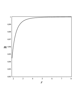
Figure 1: The behavior of the mass $m$ of the body (in units of $m_{0}$) as a function of the radial coordinate (in units of $M$) is shown for the following choice of parameters: $a/M=0.5$, $C_{Q}=1$, ${\hat{s}}=0.25$, $E/m_{0}=1$ and $J/(m_{0}M)=4$. The mass shift in this case equates $|m(+\infty)-m(r_{+})|\approx 0.055m_{0}$. The value of the dimensionless spin parameter $\hat{s}$ has been exaggerated in order to enhance the effect.

IV.3 Circular motion

IV.3.1 Solution to the order $\mathcal{O}({\hat{s}}^{2})$

In this subsection, we restrict ourselves to circular orbits, as described by the parametrizations (27)–(29). For circular motion in the equatorial plane, we must set $\alpha=\pi/2$, so that Eqs. (IV.2) become

$$\nu =\nu_{u}+\left(1-C_{Q}\right)M^{2}{\hat{s}}^{2}\left[-\nu_{\pm}(E_{\hat{r}\hat{r}}-E_{\hat{\theta}\hat{\theta}})+H_{\hat{r}\hat{\theta}}(1+\nu_{\pm}^{2})\right]\,,$$

$$\alpha_{u} =\frac{\pi}{2}\,,$$ (55)

to second order in $\hat{s}$. Thus, $F_{\rm(quad)}^{0}=0$ from its expression (53), and Eq. (52) tells us that the mass of the body is a constant of motion to that order. However, it differs from the bare mass $m_{0}$ by virtue of the general definition (48), which yields

$$m =m_{0}-\frac{1}{2}C_{Q}m_{0}M^{2}{\hat{s}}^{2}\gamma_{\pm}^{2}\left[E_{\hat{\theta}\hat{\theta}}-\nu_{\pm}^{2}E_{\hat{r}\hat{r}}+2\nu_{\pm}H_{\hat{r}\hat{\theta}}\right]$$

$$=m_{0}\left[1-\frac{1}{2}C_{Q}\frac{M^{3}}{r^{7/2}}\frac{r^{2}\mp 4a\sqrt{Mr}+3a^{2}}{r^{3/2}-3M\sqrt{r}\pm 2a\sqrt{M}}{\hat{s}}^{2}\right]\,,$$ (56)

once evaluated at $\alpha_{u}=\pi/2$, with $\nu_{u}$ replaced by $\nu_{\pm}$ to the lowest order.

Next, solving algebraically the second equation (IV.1) for $\nu_{u}$ we find

$$\nu_{u}=\nu_{\pm}+{\hat{s}}\nu_{u(1)}+{\hat{s}}^{2}\nu_{u(2)}\,,$$ (57)

where $\nu_{\pm}$ denote the geodesic linear velocities (30), while $\nu_{u(1)}$ and $\nu_{u(2)}$ are the spin-induced corrections

$$\nu_{u(1)} =\pm\frac{M}{2\zeta_{K}}[-\nu_{\pm}(E_{\hat{r}\hat{r}}-E_{\hat{\theta}\hat{\theta}})+(1+\nu_{\pm}^{2})H_{\hat{r}\hat{\theta}}]\,,$$

$$\nu_{u(2)} =\mp\frac{M^{2}}{\gamma_{\pm}^{2}\zeta_{K}}{\tilde{F}}^{1}_{\rm(quad)}$$

$$+\nu_{u(1)}\left[\nu_{u(1)}\left(\pm\frac{k_{\rm(Lie)}}{2\zeta_{K}}+\frac{1}{\nu_{\pm}}\right)\pm\left(1-C_{Q}\right)M\zeta_{K}\pm\frac{MH_{\hat{r}\hat{\theta}}}{2\gamma_{\pm}^{2}\nu_{\pm}\zeta_{K}}\right]\,,$$ (58)

of first and second orders, respectively, with (see also Eq. (E))

$${\tilde{F}}_{\rm(quad)}^{1}=\frac{1}{4}C_{Q}\left\{\gamma_{\pm}^{2}[b_{1}-b_{2}+\nu_{\pm}(b_{4}-b_{5})]-b_{1}+\frac{1}{3}(b_{2}+b_{3})\right\}\,.$$ (59)

Substituting the above solutions for $\nu_{u}$ and $\alpha_{u}$ into Eq. (IV.1) we obtain

$$E =m_{0}N\gamma_{\pm}\left(1-\frac{\sqrt{g_{\phi\phi}}N^{\phi}}{N}\nu_{\pm}\right)$$

$$+m_{0}\gamma_{\pm}\left[\gamma_{\pm}^{2}\zeta_{\pm}\nu_{u(1)}\sqrt{g_{\phi\phi}}+MN(\nu_{\pm}a(n)^{\hat{r}}+\theta_{\hat{\phi}}(n)^{\hat{r}})+M\sqrt{g_{\phi\phi}}N^{\phi}(\nu_{\pm}\theta_{\hat{\phi}}(n)^{\hat{r}}+k_{\rm(Lie)})\right]{\hat{s}}$$

$$+\left\{m_{2}N\gamma_{\pm}\left(1-\frac{\sqrt{g_{\phi\phi}}N^{\phi}}{N}\nu_{\pm}\right)+m_{0}\gamma_{\pm}^{3}\left[\sqrt{g_{\phi\phi}}\zeta_{\pm}\left(\pm M\zeta_{K}\nu_{u(1)}+\nu_{u(2)}+\frac{3}{2}\gamma_{\pm}^{2}\nu_{\pm}\nu_{u(1)}^{2}\right)+\frac{1}{2}N\nu_{u(1)}^{2}\right]\right\}{\hat{s}}^{2}\,,$$

$$J =m_{0}\gamma_{\pm}\nu_{\pm}\sqrt{g_{\phi\phi}}$$

$$+m_{0}\gamma_{\pm}\sqrt{g_{\phi\phi}}\left[\gamma_{\pm}^{2}\nu_{u(1)}-M(\nu_{\pm}\theta_{\hat{\phi}}(n)^{\hat{r}}+k_{\rm(Lie)})\right]{\hat{s}}$$

$$+\left[m_{2}\gamma_{\pm}\nu_{\pm}\sqrt{g_{\phi\phi}}+m_{0}\gamma_{\pm}^{3}\sqrt{g_{\phi\phi}}\left(\pm M\zeta_{K}\nu_{u(1)}+\nu_{u(2)}+\frac{3}{2}\gamma_{\pm}^{2}\nu_{\pm}\nu_{u(1)}^{2}\right)\right]{\hat{s}}^{2}\,.$$ (60)

The behavior of the energy $E$ versus the angular momentum $J$ in the case of co-rotating orbits is shown in Fig. 2 for selected values of the parameters.

Finally, the 4-velocity $U$ is given by Eq. (27), with normalization factor

$$\Gamma=\Gamma_{\pm}\left\{1+\gamma_{\pm}^{2}\nu_{\pm}\nu_{1}{\hat{s}}+\gamma_{\pm}^{2}\left[\nu_{\pm}\nu_{2}+\left(\frac{3}{2}\gamma_{\pm}^{2}-1\right)\nu_{1}^{2}\right]{\hat{s}}^{2}\right\}\,,$$ (61)

and angular velocity

$$\zeta=\zeta_{\pm}\left[1+\frac{N}{\zeta_{\pm}\sqrt{g_{\phi\phi}}}(\nu_{1}{\hat{s}}+\nu_{2}{\hat{s}}^{2})\right]\,,$$ (62)

where

$$\nu_{1}=\nu_{u(1)}\,,\qquad\nu_{2}=\nu_{u(2)}\pm 2\left(1-C_{Q}\right)M\zeta_{K}\nu_{1}\,.$$ (63)

The relation between the timelike unit tangent vector $U$ to the body center world line and the unit timelike vector $u$ aligned with the 4-momentum thus reads

$$U-u={\hat{s}}^{2}\gamma_{\pm}^{2}\left(1-C_{Q}\right)M\zeta_{K}\nu_{1}\bar{U}_{\pm}\,,$$ (64)

the unit vector $\bar{U}_{\pm}$ being already defined in Eq. (32). Hence, in general, $U$ and $P$ are not aligned unless $C_{Q}=1$, as discussed below.

IV.3.2 Weak field limit

Let us study now the weak field limit of the above analysis. For convenience, we introduce the dimensionless quantities $u_{0}=M/r_{0}$ and $\hat{a}=a/M$. We may consider only the case of co-rotating orbits, the counter-rotating case simply following from the replacement $\hat{a}\to-\hat{a}$. Every quantity is expanded up to a certain power of $u_{0}$ as follows

$$X\sim X_{0}+{\hat{a}}X_{\hat{a}}+{\hat{s}}X_{\hat{s}}+{\hat{a}}^{2}X_{\hat{a}\hat{a}}+2{\hat{a}}{\hat{s}}X_{\hat{a}\hat{s}}+{\hat{s}}^{2}X_{\hat{s}\hat{s}}\,,$$ (65)

where terms of orders higher than the second in the background rotation parameter, as well as terms like $\hat{a}\hat{s}^{2}$ and $\hat{a}^{2}\hat{s}$, are neglected.

The weak field expansion of the conserved energy and angular momentum (IV.3.1) are then found to be

$$\frac{E}{m_{0}} =1-\frac{1}{2}u_{0}+\frac{3}{8}u_{0}^{2}+\frac{27}{16}u_{0}^{3}+\frac{675}{128}u_{0}^{4}-\frac{1}{16}u_{0}^{5/2}(8+36u_{0}+135u_{0}^{2})(2{\hat{a}}+{\hat{s}})$$

$$+\frac{1}{4}u_{0}^{3}(2+15u_{0}){\hat{a}}^{2}+\frac{1}{4}u_{0}^{3}(2+23u_{0}){\hat{a}}{\hat{s}}+\frac{1}{8}u_{0}^{3}[2C_{Q}-(6-17C_{Q})u_{0}]{\hat{s}}^{2}+\mathcal{O}(u_{0}^{5})\,,$$

$$\frac{J}{m_{0}M} =u_{0}^{-1/2}\left(1+\frac{3}{2}u_{0}+\frac{27}{8}u_{0}^{2}+\frac{135}{16}u_{0}^{3}+\frac{2835}{128}u_{0}^{4}+\frac{15309}{256}u_{0}^{5}\right)-3u_{0}\left(1+\frac{5}{2}u_{0}+\frac{63}{8}u_{0}^{2}+\frac{405}{16}u_{0}^{3}\right){\hat{a}}$$

$$+\left(1-2u_{0}-\frac{27}{8}u_{0}^{2}-\frac{81}{8}u_{0}^{3}-\frac{4185}{128}u_{0}^{4}\right){\hat{s}}+u_{0}^{3/2}\left(1+5u_{0}+\frac{189}{8}u_{0}^{2}+\frac{405}{4}u_{0}^{3}\right){\hat{a}}^{2}$$

$$+\frac{3}{2}u_{0}^{3/2}\left(1+\frac{9}{2}u_{0}+\frac{159}{8}u_{0}^{2}+\frac{1305}{16}u_{0}^{3}\right){\hat{a}}{\hat{s}}$$

$$+\frac{3}{4}u_{0}^{3/2}\left[C_{Q}-\frac{1}{2}\left(5-\frac{23}{3}C_{Q}\right)u_{0}-\frac{1}{4}\left(7-\frac{79}{2}C_{Q}\right)u_{0}^{2}+\frac{1}{16}(81+477C_{Q})u_{0}^{3}\right]{\hat{s}}^{2}+\mathcal{O}(u_{0}^{5})\,,$$ (66)

whereas the normalization factor (61) and the angular velocity (62) become

$$\Gamma =1+\frac{3}{2}u_{0}+\frac{27}{8}u_{0}^{2}+\frac{135}{16}u_{0}^{3}+\frac{2835}{128}u_{0}^{4}-\frac{3}{16}u_{0}^{5/2}(8+36u_{0}+135u_{0}^{2})(2{\hat{a}}+{\hat{s}})$$

$$+\frac{1}{4}u_{0}^{3}(2+27u_{0}){\hat{a}}^{2}+\frac{3}{4}u_{0}^{3}(2+19u_{0}){\hat{a}}{\hat{s}}+\frac{3}{8}u_{0}^{3}[2C_{Q}+5(2+C_{Q})u_{0}]{\hat{s}}^{2}+\mathcal{O}(u_{0}^{5})\,,$$

$$M\zeta =u_{0}^{3/2}-\left({\hat{a}}+\frac{3}{2}{\hat{s}}\right)u_{0}^{3}+u_{0}^{9/2}{\hat{a}}^{2}+\frac{3}{2}u_{0}^{7/2}(1+2u_{0}){\hat{a}}{\hat{s}}+\frac{3}{4}u_{0}^{7/2}\left[C_{Q}+\left(\frac{7}{2}-2C_{Q}\right)\right]{\hat{s}}^{2}+\mathcal{O}(u_{0}^{5})\,,$$ (67)

respectively. In order to derive gauge invariant expressions, we express $E$ and $J$ in terms of the gauge-invariant dimensionless variable $y=(M\zeta)^{2/3}$, related to $u_{0}$ by

$$u_{0}=y+\left(\frac{2}{3}{\hat{a}}+{\hat{s}}\right)y^{5/2}+\frac{5}{9}y^{4}{\hat{a}}^{2}-y^{3}\left(1-\frac{5}{3}y\right){\hat{a}}{\hat{s}}-\frac{1}{2}y^{3}[C_{Q}-2(1+C_{Q})y]{\hat{s}}^{2}+\mathcal{O}(y^{9/2})\,.$$ (68)

This yields

$$\frac{E}{m_{0}} =1-\frac{1}{2}y+\frac{3}{8}y^{2}+\frac{27}{16}y^{3}+\frac{675}{128}y^{4}-y^{5/2}\left(\frac{4}{3}+4y+\frac{27}{2}y^{2}\right){\hat{a}}-y^{5/2}\left(1+\frac{3}{2}y+\frac{27}{8}y^{2}\right){\hat{s}}$$

$$+\frac{1}{2}y^{3}\left(1+\frac{65}{18}y\right){\hat{a}}^{2}+y^{3}\left(1+\frac{5}{6}y\right){\hat{a}}{\hat{s}}+\frac{1}{2}y^{3}\left[C_{Q}-5\left(1-\frac{1}{2}C_{Q}\right)y\right]{\hat{s}}^{2}+\mathcal{O}(y^{5})\,,$$

$$\frac{J}{m_{0}M} =y^{-1/2}\left(1+\frac{3}{2}y+\frac{27}{8}y^{2}+\frac{135}{16}y^{3}+\frac{2835}{128}y^{4}+\frac{15309}{256}y^{5}\right)-y\left(\frac{10}{3}+7y+\frac{81}{4}y^{2}-\frac{495}{8}y^{3}\right){\hat{a}}$$

$$+\left(1-\frac{5}{2}y-\frac{21}{8}y^{2}-\frac{81}{16}y^{3}-\frac{1485}{128}y^{4}\right){\hat{s}}+y^{3/2}\left(1+\frac{26}{9}y+\frac{335}{24}y^{2}+\frac{459}{8}y^{3}\right){\hat{a}}^{2}$$

$$+y^{3/2}\left(2+\frac{4}{3}y+\frac{25}{4}y^{2}+\frac{81}{4}y^{3}\right){\hat{a}}{\hat{s}}$$

$$+y^{3/2}\left[C_{Q}-4\left(1-\frac{1}{2}C_{Q}\right)y-\frac{15}{2}\left(1-\frac{3}{4}C_{Q}\right)y^{2}-\frac{81}{4}\left(1-\frac{5}{6}C_{Q}\right)y^{3}\right]{\hat{s}}^{2}+\mathcal{O}(y^{5})\,.$$ (69)

IV.3.3 Comparison with Ref. Hinderer et al. (2013)

Before investigating the general equatorial motion, let us show how the above analysis allows us to reproduce the results of Ref. Hinderer et al. (2013). As already stated, our quadrupole tensor reduces to the one adopted there to describe black holes if we set $C_{Q}=1$. Since we have then $\nu=\nu_{u}+\mathcal{O}({\hat{s}}^{3})$ from Eq. (IV.3.1) [see also Eq. (64)], this entails $P\propto U+\mathcal{O}({\hat{s}}^{3})$. In order to write our expressions for the energy and angular momentum in the same form as in Ref. Hinderer et al. (2013), we eliminate the dependence on the radial coordinate in favor of the angular velocity by inverting perturbatively Eq. (62):

$$r=r_{c}+\frac{M}{r_{c}}(-\sqrt{Mr_{c}}\pm a){\hat{s}}+\frac{M^{2}}{2r_{c}^{3}}\bigg{\{}\Delta_{c}-2a(a\mp\sqrt{Mr_{c}})-\left(1-C_{Q}\right)[\Delta_{c}+4a(a\mp\sqrt{Mr_{c}})]\bigg{\}}{\hat{s}}^{2}\,,$$ (70)

where $r_{c}^{3/2}=\sqrt{M}\left(\frac{1}{\zeta}\mp a\right)$ and $\Delta_{c}=\Delta(r=r_{c})$. Substituting next into Eq. (IV.3.1) leads to

$$E =\frac{m_{0}}{r_{c}^{3/4}}\frac{r_{c}^{3/2}-2M\sqrt{r_{c}}\pm a\sqrt{M}}{\left[r_{c}^{3/2}-3M\sqrt{r_{c}}\pm 2a\sqrt{M}\right]^{1/2}}\mp\frac{m_{0}M^{2}}{r_{c}^{9/4}}\frac{\sqrt{Mr_{c}}\mp a}{\left[r_{c}^{3/2}-3M\sqrt{r_{c}}\pm 2a\sqrt{M}\right]^{1/2}}{\hat{s}}$$

$$+\frac{m_{0}M^{3}}{2r_{c}^{15/4}}\frac{1}{\left[r_{c}^{3/2}-3M\sqrt{r_{c}}\pm 2a\sqrt{M}\right]^{1/2}}\Bigg{\{}r_{c}^{3/2}-4M\sqrt{r_{c}}\pm 3a\sqrt{M}$$

$$\qquad\qquad-\left(1-C_{Q}\right)\left[r_{c}^{3/2}+M\sqrt{r_{c}}\mp 9a\sqrt{M}+\frac{11a^{2}}{2\sqrt{r_{c}}}+\frac{3}{2}\frac{(r_{c}+3M)a^{2}+2M^{3/2}\sqrt{r_{c}}(\sqrt{Mr_{c}}\mp 3a)}{r_{c}^{3/2}-3M\sqrt{r_{c}}\pm 2a\sqrt{M}}\right]\Bigg{\}}{\hat{s}}^{2}\,,$$

$$J =\pm\frac{m_{0}\sqrt{M}}{r_{c}^{3/4}}\frac{r_{c}^{2}\mp 2a\sqrt{Mr_{c}}+a^{2}}{\left[r_{c}^{3/2}-3M\sqrt{r_{c}}\pm 2a\sqrt{M}\right]^{1/2}}+\frac{m_{0}M}{r_{c}^{9/4}}\frac{r_{c}^{2}(r_{c}-4M)+Ma^{2}\pm a\sqrt{Mr_{c}}(3r_{c}-M)}{\left[r_{c}^{3/2}-3M\sqrt{r_{c}}\pm 2a\sqrt{M}\right]^{1/2}}{\hat{s}}$$

$$\pm\frac{m_{0}M^{5/2}}{2r_{c}^{15/4}}\frac{1}{\left[r_{c}^{3/2}-3M\sqrt{r_{c}}\pm 2a\sqrt{M}\right]^{1/2}}\Bigg{\{}3Ma^{2}\pm 2a\sqrt{Mr_{c}}(3r_{c}-2M)+r_{c}^{2}(2r_{c}-7M)$$

$$\left.\qquad\qquad-\left(1-C_{Q}\right)\left[(2r_{c}+3M)(r_{c}^{2}-Mr_{c}+3M^{2})\mp 4a\sqrt{Mr_{c}}(3r_{c}+2M)+10r_{c}a^{2}\pm\frac{11\sqrt{M}a^{3}}{2\sqrt{r_{c}}}\right.\right.$$

$$\left.\qquad\qquad+\frac{3}{2}\sqrt{M}\frac{6M^{3/2}\sqrt{r_{c}}(3M^{2}+4a^{2})\mp a[a^{2}(r_{c}+9M)+4M^{2}(5r_{c}+3M)]}{r_{c}^{3/2}-3M\sqrt{r_{c}}\pm 2a\sqrt{M}}\right]\Bigg{\}}{\hat{s}}^{2}\,.$$ (71)

This exactly reproduces the results of Ref. Hinderer et al. (2013) when specialized to the case $C_{Q}=1$ [see their counterparts displayed in Eqs. (39a) and (39b) there, with in addition $M=1=m_{0}$].

$\begin{array}[]{cc}\includegraphics[scale={0.3}]{fig2a}&\quad\includegraphics[scale={0.3}]{fig2b}\\[11.38092pt] \quad\mbox{(a)}&\quad\mbox{(b)}\end{array}$

Figure 2: The behavior of the energy $E$ versus the angular momentum $J$ in the case of co-rotating circular orbits is shown in panel (a), for the fixed black-hole dimensionless spin parameter $a/M=0.5$ and different values of $\hat{s}$; in panel (b), for the fixed body spin $\hat{s}=0.25$ and different values of $a/M$; $C_{Q}=1$ in both cases. Dashed curves in (b) correspond to the geodesic motion ($\hat{s}=0$).

IV.4 General equatorial motion

IV.4.1 Effective potential

In order to discuss the general features of equatorial motion it is most useful to introduce appropriate effective potentials Landau and Lifshitz (1975); Misner et al. (1973). The latter naturally arise when factoring the expression of $({{\rm d}r}/{{\rm d}\tau})^{2}$ as a polynomial in the energy $E$ of the test object. This factorisation takes the form

$$\left(\frac{{\rm d}r}{{\rm d}\tau}\right)^{2}=\frac{\gamma^{2}\nu^{2}\cos^{2}\alpha}{g_{rr}}={\mathcal{A}}\,{\mathcal{P}}(E)(E-V_{(+)})(E-V_{(-)})+O({\hat{s}}^{3})\,,$$ (72)

where the solutions for $\nu$ and $\alpha$ in terms of the conserved energy and angular momentum are given by Eqs. (IV.2)–(IV.2). More precisely, we find

$${\mathcal{A}} =\frac{1}{m_{0}^{2}N^{2}g_{rr}}\bigg{\{}1-2M{\hat{s}}\theta_{\hat{\phi}}(n)^{\hat{r}}-M^{2}{\hat{s}}^{2}\bigg{[}k_{\rm(Lie)}(k_{\rm(Lie)}-a(n)^{\hat{r}})$$

$$\qquad\qquad\qquad\qquad+(2-C_{Q})(2E_{\hat{r}\hat{r}}+E_{\hat{\theta}\hat{\theta}})\frac{J^{2}}{m_{0}^{2}g_{\phi\phi}}+(3-C_{Q})E_{\hat{\theta}\hat{\theta}}+3E_{\hat{r}\hat{r}}\bigg{]}\bigg{\}}\,,$$

$${\mathcal{P}}(E) =1+\frac{M^{2}{\hat{s}}^{2}}{m_{0}^{2}N^{2}}(2-C_{Q})(E+N^{\phi}J)\left[(E_{\hat{r}\hat{r}}+2E_{\hat{\theta}\hat{\theta}})(E+N^{\phi}J)+2\frac{N}{\sqrt{g_{\phi\phi}}}H_{\hat{r}\hat{\theta}}J\right]\,,$$ (73)

and

$$V_{(\pm)}=V_{0}^{(\pm)}+{\hat{s}}V_{1}^{(\pm)}+{\hat{s}}^{2}V_{2}^{(\pm)}\,,$$ (74)

with

$$V_{0}^{(\pm)} =-N^{\phi}J\pm\frac{N}{\sqrt{g_{\phi\phi}}}\sqrt{m_{0}^{2}g_{\phi\phi}+J^{2}}\,,$$

$$V_{1}^{(\pm)} =\frac{MN}{\sqrt{g_{\phi\phi}}}\left[(a(n)^{\hat{r}}+k_{\rm(Lie)})J\pm\theta_{\hat{\phi}}(n)^{\hat{r}}\frac{m_{0}^{2}g_{\phi\phi}+2J^{2}}{\sqrt{m_{0}^{2}g_{\phi\phi}+J^{2}}}\right]\,,$$

$$V_{2}^{(\pm)} =\pm\frac{M^{2}N}{2\sqrt{g_{\phi\phi}}}\bigg{\{}\pm 2[\theta_{\hat{\phi}}(n)^{\hat{r}}(a(n)^{\hat{r}}+3k_{\rm(Lie)})-C_{Q}H_{\hat{r}\hat{\theta}}]J$$

$$\qquad\qquad\quad+\sqrt{m_{0}^{2}g_{\phi\phi}+J^{2}}\left[2k_{\rm(Lie)}(k_{\rm(Lie)}+3a(n)^{\hat{r}})-(4-C_{Q})E_{\hat{r}\hat{r}}-(4+C_{Q})E_{\hat{\theta}\hat{\theta}}\right]\bigg{\}}$$

$$\mp\frac{M^{2}m_{0}^{2}N\sqrt{g_{\phi\phi}}}{2\sqrt{m_{0}^{2}g_{\phi\phi}+J^{2}}}\bigg{\{}[k_{\rm(Lie)}(k_{\rm(Lie)}+3a(n)^{\hat{r}})-(3-C_{Q})E_{\hat{r}\hat{r}}-3E_{\hat{\theta}\hat{\theta}}]$$

$$+\frac{m_{0}^{2}g_{\phi\phi}}{m_{0}^{2}g_{\phi\phi}+J^{2}}[k_{\rm(Lie)}a(n)^{\hat{r}}-(E_{\hat{r}\hat{r}}+E_{\hat{\theta}\hat{\theta}})]\bigg{\}}\,.$$ (75)

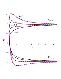
Figure 3: The behavior of the effective potential for radial motion is shown for the following choice of parameters: $a/M=0.5$, $C_{Q}=1$, $\hat{s}=0.25$, and for different values of the body dimensionless angular momentum, $J/(m_{0}M)=[1,2.5,4,6]$. The corresponding geodesic case ($\hat{s}=0$) is also shown for comparison (dashed curves).

If $E$ and $J$ are kept fixed as $\hat{s}$ goes to zero, the leading order approximation of $\mathcal{P}(E)$ is obtained by setting exactly $\hat{s}=0$ in Eq. (IV.4.1), which shows that $\mathcal{P}(E)$ is necessarily positive in the domain of validity of the small spin expansion. The solutions $E=V_{(\pm)}$ are generalizations of the radial effective potentials for a test particle in a Kerr spacetime to the case of an extended body with spin-induced quadrupole moment. Their behavior as a function of the radial distance is shown in Fig. 3 for selected values of the parameters. The upper/lower branch corresponds to the $+$/$-$ sign in Eq. (IV.4.1).

On the other hand, since the equation $({{\rm d}r}/{{\rm d}\tau})^{2}=0$ is quartic in $E$, in order to give a complete account of effective potentials we should also consider the solutions to the equation ${\mathcal{P}}(E)=0$, or equivalently,

$$1+\frac{3aM^{3}{\hat{s}}^{2}}{m_{0}^{2}r^{5}}(2-C_{Q})(E+N^{\phi}J)\left[a(E+N^{\phi}J)-2\frac{N^{2}}{\Delta}(r^{2}+a^{2})J\right]=0\,.$$ (76)

If $C_{Q}<2$, no real solutions for the energy exist. If $C_{Q}=2$, then ${\mathcal{P}}(E)=1$, irrespective of $E$ and $J$. If $C_{Q}>2$ (so excluding the black hole case $C_{Q}=1$), the above equation admits two real solutions $E=W_{(\pm)}$, perturbatively in ${\hat{s}}$, only if $E$ scales as $1/\hat{s}$, with

$$W_{(\pm)}=\frac{m_{0}}{\hat{a}}\left[\pm\frac{1}{{\hat{s}}\sqrt{3(C_{Q}-2)}}\left(\frac{r}{M}\right)^{5/2}+\frac{J}{m_{0}M}\right]+O({\hat{s}})\,.$$ (77)

Note that the solutions $W_{(\pm)}$ diverge in both limits ${\hat{a}}\to 0$ and ${\hat{s}}\to 0$ for fixed values of the radial distance. Furthermore, for fixed values of the dimensionless spin parameters, they indefinitely grow for large $r$, exhibiting a monotonic behavior $W_{(\pm)}\sim\pm({r}/{M})^{5/2}$, so that there cannot exist circular orbits associated with them. In the following, we shall actually exclude the configurations for which $E=\mathcal{O}(1/\hat{s})$ and ignore both potentials $W_{(\pm)}$.

IV.4.2 Circular orbits and ISCO

Circular orbits correspond to the extremal points of $V_{(+)}$ and solving for $J$ the resulting equation, $V_{(+)}^{\prime}=0$, provides the associated angular momentum. Now, as pointed out by Le Tiec et al. Le Tiec et al. (2012), the shift of the ISCO frequency due to the peturbation induced to the spacetime background metric by the particle itself is an important strong-field benchmark. Gravitational self-force theory has provided very accurate analytic predictions for it in the case of a spinless body in motion along a circular geodesic on a Schwarzschild background, at the first order in the symmetric mass ratio of the two objects. In the present situation, because of its spinning and quadrupolar structure, the body deviates from geodesic motion in the way described by the MPD model. As a result, the last stable circular orbit undergoes a shift in the frequency, made of terms proportional to the spin as well as the quadrupole. Measuring this effect can therefore provide relevant information on the structure of the body. Conversely, having information about the spin and quadrupolar structure of the body allows one to make predictions on the frequency of circular motion and its deviation from the corresponding geodesic value.

Stability requires that $V_{(+)}^{\prime\prime}\leq 0$. For a spinless object the latter condition boils down to

$$r^{2}-6Mr-3a^{2}\pm 8a\sqrt{Mr}\geq 0\,.$$ (78)

The equality can be analytically solved for the radius $r_{\rm ms}$ of the marginally stable orbit (or ISCO) Bardeen et al. (1972):

$$r_{\rm ms}^{\rm Kerr}=M\left[3+Z_{2}\mp\sqrt{(3-Z_{1})(3+Z_{1}+2Z_{2})}\right]\,,$$ (79)

where the upper/lower sign refers to co/counter-rotating orbits, with

$$Z_{1}=1+\left(1-{\hat{a}}^{2}\right)^{1/3}\left[\left(1-{\hat{a}}\right)^{1/3}+\left(1+{\hat{a}}\right)^{1/3}\right]\,,\quad Z_{2}=\sqrt{3{\hat{a}}^{2}+Z_{1}^{2}}\,.$$ (80)

The latter quantities are even functions of ${\hat{a}}$ satisfying $Z_{2}\geq Z_{1}$, $Z_{1}\leq 3$ and, for ${\hat{a}}=0$, $Z_{1}=3=Z_{2}$. For small values of ${\hat{a}}$, the Kerr ISCO radius may be expanded as

$$\frac{r_{\rm ms}^{\rm Kerr}}{M}=6\mp\frac{4\sqrt{6}}{3}{\hat{a}}-\frac{7}{18}{\hat{a}}^{2}\mp\frac{13\sqrt{6}}{162}{\hat{a}}^{3}-\frac{241}{1944}{\hat{a}}^{4}+O({\hat{a}}^{5})\,.$$ (81)

We recover the value $r_{\rm ms}^{\rm Kerr}=6M$ in the Schwarzschild case (${\hat{a}}=0$).

For a spinning particle the ISCO is modified as follows:

$$r_{\rm ISCO}=r_{{\rm ms}}^{\rm Kerr}+{\hat{s}}r_{{\rm ms}(1)}+{\hat{s}}^{2}r_{{\rm ms}(2)}\,,$$ (82)

where

$$\frac{r_{{\rm ms}(1)}}{M} =\mp\frac{2\sqrt{6}}{3}+\frac{2}{9}{\hat{a}}\pm\frac{17\sqrt{6}}{324}{\hat{a}}^{2}+\frac{43}{486}{\hat{a}}^{3}+O({\hat{a}}^{4})\,,$$

$$\frac{r_{{\rm ms}(2)}}{M} =-\frac{29}{72}+\frac{1}{2}C_{Q}\pm\frac{\sqrt{6}}{54}\left(\frac{23}{24}+C_{Q}\right){\hat{a}}+\frac{1}{81}\left(\frac{451}{48}-4C_{Q}\right){\hat{a}}^{2}\pm\frac{\sqrt{6}}{1296}\left(\frac{4559}{72}-37C_{Q}\right){\hat{a}}^{3}+O({\hat{a}}^{4})\,.$$ (83)

Of course, both the first and second order corrections to the ISCO can also be straightforwardly computed in the strong field regime. However, the corresponding expressions are quite long, so we prefer not to explicitly write them down. For instance, in the co-rotating case, for ${\hat{a}}=0.5$, we find $r_{{\rm ms}}^{\rm Kerr}/M\approx 4.233$, $r_{{\rm ms}(1)}/M\approx-1.472$ and $r_{{\rm ms}(2)}/M\approx 0.194$ ($C_{Q}=1$), or $r_{{\rm ms}(2)}/M\approx 2.674$ ($C_{Q}=6$). The resulting behavior of $r_{\rm ISCO}$ as a function of the spin parameter ${\hat{s}}$ is shown in Fig. 4.

The ISCO frequency of a spinning test object is then computed to be

$$M\zeta_{\rm ISCO}=\pm 6^{-3/2}\left\{1\pm\frac{1}{\sqrt{6}}\left(\frac{11}{6}{\hat{a}}+\frac{3}{4}{\hat{s}}\right)+\frac{59}{108}{\hat{a}}^{2}+\frac{1}{3}{\hat{a}}{\hat{s}}+\frac{1}{9}\left(\frac{97}{64}-C_{Q}\right){\hat{s}}^{2}\right\}\,,$$ (84)

leading to a fractional correction with respect to the spinless case

$$\delta_{\rm ISCO}\equiv\frac{\zeta_{\rm ISCO}}{\zeta_{\rm ISCO}^{\rm Kerr}}-1=\pm\frac{\sqrt{6}}{8}{\hat{s}}+\frac{5}{48}{\hat{a}}{\hat{s}}+\frac{1}{9}\left(\frac{97}{64}-C_{Q}\right){\hat{s}}^{2}\,,$$ (85)

whereas the energy and angular momentum at the ISCO read

$$\frac{E_{\rm ISCO}}{m_{0}} =\frac{2\sqrt{2}}{3}\mp\frac{\sqrt{3}}{108}(2{\hat{a}}+{\hat{s}})-\frac{2\sqrt{2}}{3}\left[\frac{5}{216}{\hat{a}}^{2}+\frac{1}{54}{\hat{a}}{\hat{s}}+\frac{1}{216}\left(\frac{15}{8}-C_{Q}\right){\hat{s}}^{2}\right]\,,$$

$$\frac{J_{\rm ISCO}}{m_{0}M} =\pm 2\sqrt{3}-\frac{\sqrt{2}}{3}(2{\hat{a}}-{\hat{s}})\mp 2\sqrt{3}\left[\frac{2}{27}{\hat{a}}^{2}+\frac{11}{216}{\hat{a}}{\hat{s}}+\frac{1}{24}\left(1-\frac{7}{9}C_{Q}\right){\hat{s}}^{2}\right]\,.$$ (86)

The behavior of the ISCO frequency as a function of the spin parameter ${\hat{s}}$ is shown in Fig. 5 for two typical values of $C_{Q}$, i.e., $C_{Q}=1$ (black hole) and $C_{Q}=6$ (neutron star). The corresponding curve is in general a parabola, which is concave up or down depending on whether the sign of the coefficient of ${\hat{s}}^{2}$ is positive or negative. For instance, for the chosen values of the rotation parameter ${\hat{a}}=[0,0.5,0.9]$, the change of concavity (from up to down) occurs at $C_{Q}\approx[1.516,1.487,1.455]$, respectively. Finally, Fig. 6 shows the behavior of the fractional correction to the ISCO frequency as a function of the spin parameter. Furthermore, restricting $\hat{s}$ to a given range of values yields the uncertainty associated with the ISCO position, angular velocity and shift. As an example, we list the three latter quantities below in Table 1 for selected values of the rotational parameter ${\hat{a}}=[0,0.1,0.3,0.5,0.7,0.9]$, spin parameter ${\hat{s}}=[-0.1,0,0.1]$ and polarizability parameter $C_{Q}=[1,6]$, in the corotating case.

$\begin{array}[]{cc}\includegraphics[scale={0.3}]{fig4a}&\quad\includegraphics[scale={0.3}]{fig4b}\\[11.38092pt] \quad\mbox{(a)}&\quad\mbox{(b)}\end{array}$

Figure 4: The radius of the ISCO as a function of the spin parameter is shown in the case of co-rotating orbits for different values of the black-hole dimensionless spin, $a/M=[0,0.5,0.9]$, and for (a) $C_{Q}=1$, as well as (b) $C_{Q}=6$.

$\begin{array}[]{cc}\includegraphics[scale={0.3}]{fig5a}&\quad\includegraphics[scale={0.3}]{fig5b}\\[11.38092pt] \quad\mbox{(a)}&\quad\mbox{(b)}\end{array}$

Figure 5: The behavior of the ISCO frequency as a function of the spin parameter is shown in the case of co-rotating orbits for different values of the black-hole spin, $a/M=[0,0.5,0.9]$, and for (a) $C_{Q}=1$, as well as (b) $C_{Q}=6$.

$\begin{array}[]{cc}\includegraphics[scale={0.3}]{fig6a}&\quad\includegraphics[scale={0.3}]{fig6b}\\[11.38092pt] \quad\mbox{(a)}&\quad\mbox{(b)}\end{array}$

Figure 6: The behavior of the fractional correction to the ISCO frequency as a function of the spin parameter is shown in the case of co-rotating orbits for different values of the black-hole dimensionless spin, $a/M=[0,0.5,0.9]$, and for (a) $C_{Q}=1$, as well as (b) $C_{Q}=6$.

Table 1: The numerical values for the modified ISCO position, angular velocity and shift are listed for selected values of ${\hat{s}}$ and ${\hat{a}}$ in the corotating case, for $C_{Q}=1$ (black hole), as well as $C_{Q}=6$ (neutron star).

$C_{Q}=1$
	$r_{\rm ISCO}/M$			$M\zeta_{\rm ISCO}$			$\delta_{\rm ISCO}$
	$-0.1$	0	0.1	$-0.1$	0	0.1	$-0.1$	0	0.1
0	6.1643	6	5.8377	0.0660	0.0680	0.0702	$-0.0300$	0	0.0312
0.1	5.8313	5.6693	5.5094	0.0712	0.0735	0.0759	$-0.0311$	0	0.0323
0.3	5.1351	4.9786	4.8248	0.0847	0.0877	0.0907	$-0.0335$	0	0.0348
0.5	4.3824	4.2330	4.0876	0.1046	0.1086	0.1127	$-0.0365$	0	0.0376
0.7	3.5259	3.3931	3.3002	0.1384	0.1439	0.1475	$-0.0379$	0	0.0250
0.9	2.4018	2.3209	2.2427	0.2194	0.2254	0.2317	$-0.0267$	0	0.0277
$C_{Q}=6$
	$r_{\rm ISCO}/M$			$M\zeta_{\rm ISCO}$			$\delta_{\rm ISCO}$
	$-0.1$	0	0.1	$-0.1$	0	0.1	$-0.1$	0	0.1
0	6.1893	6	5.8627	0.0656	0.0680	0.0698	-0.0356	0	0.0256
0.1	5.8565	5.6693	5.5346	0.0708	0.0735	0.0755	$-0.0370$	0	0.0264
0.3	5.1604	4.9786	4.8501	0.0841	0.0877	0.0901	$-0.0402$	0	0.0281
0.5	4.4065	4.2330	4.1122	0.1038	0.1086	0.1119	$-0.0438$	0	0.0301
0.7	3.5438	3.3931	3.2815	0.1375	0.1439	0.1486	$-0.0446$	0	0.0330
0.9	2.4094	2.3209	2.2504	0.2184	0.2254	0.2306	$-0.0313$	0	0.0230

IV.4.3 Quasi-circular orbits

Let us finally construct the quadratic-in-spin solution to the MPD equations corresponding to a quasi-circular orbit, in the perturbative sense. The initial conditions are chosen so that the world line of the extended body has the same starting point as the reference circular geodesic at radius $r=r_{0}$ for vanishing spin. We also require that the two world lines are initially tangent.

The orbit can be parametrized in a Keplerian-like form as follows Damour and Deruelle (1985); Schäfer and Wex (1993)

$$\frac{2\pi}{P}(t-t_{0}) =\ell_{t}-e_{t}\sin\ell_{t}\,,$$

$$\qquad\quad\quad r =a_{r}(1-e_{r}\cos\ell_{r})\,,$$

$$\qquad\quad\quad\theta =\frac{\pi}{2}\,,$$

$$\frac{2\pi}{\Phi}(\phi-\phi_{0}) =2\arctan\left(\sqrt{\frac{1+e_{\phi}}{1-e_{\phi}}}\tan\frac{\ell_{\phi}}{2}\right)\,,$$ (87)

where $a_{r}$ is some “semimajor axis”, $e_{t}$, $e_{r}$ and $e_{\phi}$ are three different “eccentricities”, which would coincide in the Newtonian theory, while $P$ and $\Phi$ denote the periods of $t$ and $\phi$ motions, respectively (with an abuse of notation for $P$, not to be confused with the body’s 4-momentum). The quantities $\ell_{t}$, $\ell_{r}$ and $\ell_{\phi}$ are functions of the proper time parameter $\tau$ on the orbit. They are conveniently expressed in terms of the dimensionless variable $\ell=\Omega_{\rm(ep)}\tau$, where

$$\Omega_{\rm(ep)}=|\Omega_{\pm}|\left[1-\frac{6M}{r_{0}}-\frac{3a^{2}}{r_{0}^{2}}\pm 8a\zeta_{K}\right]^{1/2}$$ (88)

denotes the well-known epicyclic frequency governing the radial perturbations of circular geodesics. The quantities $\ell_{t}$, $\ell_{r}$, $\ell_{\phi}$ and $\ell$ play the role of eccentric anomalies. Note that, for geodesics, the above quantities reduce to $a_{r}=r_{0}$, $e_{t}=e_{r}=e_{\phi}=0$, $P=2\pi\Gamma_{\pm}$, $\Phi=2\pi\Omega_{\pm}$ and $\ell_{t}=\ell_{r}=\ell_{\phi}=\ell$. For non-vanishing spin parameter $\hat{s}$, the semimajor axis and the eccentricities for the orbit of the extended body turn out to be

$$a_{r}=r_{0}-{\hat{s}}R_{\hat{s}}-{\hat{s}}^{2}C_{1{\hat{s}}}\,,$$ (89)

and

$$e_{t} =-\frac{\Omega_{\rm(ep)}}{\Gamma_{\pm}}{\hat{s}}\left[T_{\hat{s}}+{\hat{s}}\left(D_{1{\hat{s}}}+\frac{\Omega_{\rm(ep)}}{\Gamma_{\pm}}T_{\hat{s}}^{2}\right)\right]\,,$$

$$e_{r} =-\frac{{\hat{s}}}{r_{0}}\left[R_{\hat{s}}+{\hat{s}}\left(C_{1{\hat{s}}}+\frac{R_{\hat{s}}^{2}}{r_{0}}\right)\right]\,,$$ (90)

$$e_{\phi} =\frac{\Omega_{\rm(ep)}}{\Omega_{\pm}}{\hat{s}}\left[\bar{\zeta}_{\pm}T_{\hat{s}}+{\hat{s}}\left(E_{1{\hat{s}}}+\frac{\Omega_{\rm(ep)}}{\Omega_{\pm}}\bar{\zeta}_{\pm}^{2}T_{\hat{s}}^{2}\right)\right]\,,$$

respectively. As for the periods of $t$ and $\phi$ motions, they may be written as

$$P =2\pi\frac{\Gamma_{\pm}}{\Omega_{\rm(ep)}}\left[1\mp 2\gamma_{\pm}\nu_{\pm}\frac{\zeta_{K}}{\Omega_{\rm(ep)}}{\mathcal{V}}^{(r)}_{\hat{s}}{\hat{s}}+\frac{D_{4{\hat{s}}}}{\Gamma_{\pm}}{\hat{s}}^{2}\right]\,,$$

$$\Phi =2\pi\frac{\Omega_{\pm}}{\Omega_{\rm(ep)}}\left[1\mp 2\gamma_{\pm}\nu_{\pm}\frac{\zeta_{K}}{\Omega_{\rm(ep)}}\frac{\bar{\zeta}_{\pm}}{\zeta_{\pm}}{\mathcal{V}}^{(r)}_{\hat{s}}{\hat{s}}+\frac{E_{4{\hat{s}}}}{\Omega_{\pm}}{\hat{s}}^{2}\right]\,.$$ (91)

There remains to display the three eccentric anomaly parameters, $\ell_{t}$, $\ell_{r}$ and $\ell_{\phi}$, as functions of $\ell$:

$$\ell_{t} =\ell+\frac{{\hat{s}}^{2}}{\Gamma_{\pm}}[D_{2{\hat{s}}}\Omega_{\rm(ep)}\sin 2\ell+D_{3{\hat{s}}}\ell\cos\ell]\,,$$

$$\ell_{r} =\ell+\frac{{\hat{s}}}{R_{\hat{s}}\Omega_{\rm(ep)}}[2C_{2{\hat{s}}}\Omega_{\rm(ep)}\sin\ell-C_{3{\hat{s}}}\ell]\,,$$

$$\ell_{\phi} =\ell+\frac{{\hat{s}}^{2}}{\Omega_{\pm}}\left[\Omega_{\rm(ep)}\left(E_{2{\hat{s}}}-\frac{1}{4}\Omega_{\rm(ep)}^{2}\bar{\zeta}_{\pm}^{2}T_{\hat{s}}^{3}\right)\sin 2\ell+E_{3{\hat{s}}}\ell\cos\ell\right]\,.$$ (92)

The various coefficients entering the above formulas are listed in Appendix E. Notice that the parametrization (IV.4.3) of the orbit is different from the quasi-Keplerian one, used in Refs. Damour and Deruelle (1985); Schäfer and Wex (1993), due to the presence of different parameters representing the $t$, $r$ and $\phi$ motions instead of a single eccentric anomaly. The two forms agree to first order in spin only, as shown in Ref. Bini and Geralico (2014a).

At this stage, we can derive explicit expressions for the conserved energy and angular momentum (II.3):

$$\tilde{E}\equiv\frac{E}{m_{0}}=\tilde{E}_{\pm}+{\hat{s}}\tilde{E}_{\hat{s}}+{\hat{s}}^{2}\tilde{E}_{\hat{s}\hat{s}}\,,\qquad\tilde{J}\equiv\frac{J}{m_{0}}=\tilde{L}_{\pm}+{\hat{s}}\tilde{J}_{\hat{s}}+{\hat{s}}^{2}\tilde{J}_{\hat{s}\hat{s}}\,,$$ (93)

with

$$\tilde{E}_{\hat{s}}=M\Omega_{\pm}\left(\frac{M}{r_{0}}\mp a\zeta_{K}\right)\,,\qquad\tilde{E}_{\hat{s}}-\zeta_{\pm}\tilde{J}_{\hat{s}}=\mp\frac{M\zeta_{K}}{\Gamma_{\pm}}\,,$$ (94)

and

$$\tilde{J}_{\hat{s}\hat{s}}=-\sqrt{g_{\phi\phi}}\gamma_{\pm}^{2}{\mathcal{V}}^{(r)}_{\hat{s}}\left[\left(1-C_{Q}\right)M\Omega_{\rm(ep)}+\frac{2}{\gamma_{\pm}\nu_{\pm}}{\mathcal{V}}^{(r)}_{\hat{s}}\right]+\frac{m_{2}}{m_{0}}\tilde{L}_{\pm}\,,$$

$$\tilde{E}_{\hat{s}\hat{s}}-\zeta_{\pm}\tilde{J}_{\hat{s}\hat{s}}=2N\gamma_{\pm}({\mathcal{V}}^{(r)}_{\hat{s}})^{2}+\frac{m_{2}}{m_{0}}\frac{1}{\Gamma_{\pm}}\,,$$ (95)

where $\tilde{E}_{\pm}$ and $\tilde{L}_{\pm}$ are the energy and the azimuthal angular momentum per unit (bare) mass for a circular geodesic, as given by Eqs. (III), the parameter $m_{2}$ representing the spin correction (51) to the mass of the body [see also Eq. (IV.3.1)].

In the weak field limit the previous expressions become

$$-2{\widehat{E}}\equiv -2(\tilde{E}-1)=u_{0}\left(1-\frac{3}{4}u_{0}-\frac{27}{8}u_{0}^{2}-\frac{675}{64}u_{0}^{3}\right)+2u_{0}^{5/2}\left(1+\frac{9}{2}u_{0}+\frac{135}{8}u_{0}^{2}\right){\hat{a}}$$

$$\qquad\qquad\quad-2u_{0}^{5/2}\left(1+\frac{3}{2}u_{0}+\frac{27}{8}u_{0}^{2}\right){\hat{s}}-u_{0}^{3}\left(1+\frac{15}{2}u_{0}\right){\hat{a}}^{2}+2u_{0}^{3}\left(1+\frac{5}{2}u_{0}\right){\hat{a}}{\hat{s}}$$

$$\qquad\qquad\quad+u_{0}^{3}\left[C_{Q}+6\left(1+\frac{5}{12}C_{Q}\right)u_{0}\right]{\hat{s}}^{2}+O(u_{0}^{5})\,,$$

$${\widehat{J}}\equiv \frac{\tilde{J}}{M}=u_{0}^{-1/2}\left(1+\frac{3}{2}u_{0}+\frac{27}{8}u_{0}^{2}+\frac{135}{16}u_{0}^{3}+\frac{2835}{128}u_{0}^{4}\right)-3u_{0}\left(1+\frac{5}{2}u_{0}+\frac{63}{8}u_{0}^{2}+\frac{405}{16}u_{0}^{3}\right){\hat{a}}$$

$$\quad\leavevmode\nobreak\ +\left(1-\frac{1}{2}u_{0}+\frac{3}{8}u_{0}^{2}+\frac{27}{16}u_{0}^{3}+\frac{675}{128}u_{0}^{4}\right){\hat{s}}+u_{0}^{3/2}\left(1+5u_{0}+\frac{189}{8}u_{0}^{2}+\frac{405}{4}u_{0}^{3}\right){\hat{a}}^{2}-3u_{0}^{7/2}{\hat{a}}{\hat{s}}$$

$$\quad\leavevmode\nobreak\ -21u_{0}^{5/2}\left[1+\frac{1}{42}C_{Q}+\frac{1}{14}\left(71+\frac{3}{2}C_{Q}\right)u_{0}+\frac{15}{56}\left(111+\frac{3}{2}C_{Q}\right)u_{0}^{2}\right]{\hat{s}}^{2}+O(u_{0}^{5})\,,$$ (96)

for the co-rotating case. We list below the orbital elements (89)–(IV.4.3) expressed in terms of the gauge invariant quantities ${\widehat{E}}$ and ${\widehat{J}}$, related by

$${\widehat{J}} =(-2{\widehat{E}})^{-1/2}\left\{1+\frac{9}{8}(-2{\widehat{E}})+\frac{243}{128}(-2{\widehat{E}})^{2}+\frac{5373}{1024}(-2{\widehat{E}})^{3}-2(-2{\widehat{E}})^{3/2}\left[1+\frac{9}{4}(-2{\widehat{E}})+\frac{81}{8}(-2{\widehat{E}})^{2}\right]{\hat{a}}\right.$$

$$\left.\qquad\qquad\qquad+(-2{\widehat{E}})^{1/2}\left[1-\frac{3}{2}(-2{\widehat{E}})-\frac{9}{4}(-2{\widehat{E}})^{2}-\frac{81}{8}(-2{\widehat{E}})^{3}\right]{\hat{s}}+\frac{1}{2}(-2{\widehat{E}})^{2}\left[1+\frac{69}{8}(-2{\widehat{E}})\right]{\hat{a}}^{2}\right.$$

$$\left.\qquad\qquad\qquad+(-2{\widehat{E}})^{2}\left[1+\frac{45}{8}(-2{\widehat{E}})\right]{\hat{a}}{\hat{s}}+\frac{1}{2}(-2{\widehat{E}})^{2}\left[C_{Q}-3\left(15-\frac{7}{8}C_{Q}\right)(-2{\widehat{E}})\right]{\hat{s}}^{2}+O[(-2{\widehat{E}})^{4}]\right\}\,,$$ (97)

so that we may write them with the help of a single parameter, e.g., the energy parameter $(-2{\widehat{E}})\equiv X$. We find

$$\frac{a_{r}}{M} =X^{-1}\left(1-\frac{3}{4}X-\frac{63}{16}X^{2}-\frac{1215}{64}X^{3}-\frac{27135}{256}X^{4}\right)+X^{1/2}\left(1+\frac{51}{8}X+\frac{5751}{128}X^{2}\right)(2{\hat{a}}+{\hat{s}})$$

$$-X\left(1+\frac{63}{4}X+183X^{2}\right){\hat{a}}^{2}-X\left(1+\frac{79}{4}X+213X^{2}\right){\hat{a}}{\hat{s}}$$

$$-\frac{1}{2}X\left[C_{Q}-\left(36+\frac{5}{4}C_{Q}\right)X-3\left(86-\frac{1}{2}C_{Q}\right)X^{2}\right]{\hat{s}}^{2}+O(X^{7/2})\,,$$

$$e_{t} =-6X^{5/2}\left\{\left(1+\frac{63}{8}X\right){\hat{s}}-X^{1/2}\left(1+\frac{97}{4}X\right){\hat{a}}{\hat{s}}-\frac{1}{2}X^{1/2}\left[C_{Q}+\left(1+\frac{25}{4}C_{Q}\right)X\right]{\hat{s}}^{2}+O(X^{2})\right\}\,,$$

$$e_{r} =3X^{3/2}\left\{\left(1+\frac{41}{8}X\right){\hat{s}}-X^{1/2}\left(1+\frac{33}{2}X\right){\hat{a}}{\hat{s}}-\frac{1}{2}X^{1/2}\left[C_{Q}-\left(10-\frac{7}{2}C_{Q}\right)X\right]{\hat{s}}^{2}+O(X^{2})\right\}\,,$$

$$e_{\phi} =6X^{3/2}\left\{\left(1+\frac{41}{8}X\right){\hat{s}}-X^{1/2}\left(1+\frac{31}{2}X\right){\hat{a}}{\hat{s}}-\frac{1}{2}X^{1/2}\left[C_{Q}-\left(4-\frac{7}{2}C_{Q}\right)X\right]{\hat{s}}^{2}+O(X^{2})\right\}\,.$$ (98)

At last, the periods of $t$ and $\phi$ motions are given by

$$\frac{1}{M}\frac{P}{2\pi} =X^{-3/2}\left\{1+\frac{15}{8}X+\frac{855}{128}X^{2}+\frac{41175}{1024}X^{3}-12X^{5/2}\left(1+\frac{51}{4}X\right){\hat{a}}-3X^{3/2}(1+6X+39X^{2}){\hat{s}}\right.$$

$$\left.\qquad\qquad\,+11X^{3}{\hat{a}}^{2}+3X^{2}\left(1+\frac{99}{8}X\right){\hat{a}}{\hat{s}}+\frac{3}{2}X^{2}\left[C_{Q}+\left(1+\frac{59}{8}C_{Q}\right)X\right]{\hat{s}}^{2}+O(X^{4})\right\}\,,$$

$$\frac{\Phi}{2\pi} =1+3X+\frac{63}{4}X^{2}+\frac{405}{4}X^{3}-4X^{3/2}\left(1+\frac{93}{8}X\right){\hat{a}}-6X^{3/2}\left(1+\frac{57}{8}X\right){\hat{s}}$$

$$+\frac{3}{2}X^{2}\left(1+\frac{73}{2}X\right){\hat{a}}^{2}+6X^{2}\left(1+\frac{39}{2}X\right){\hat{a}}{\hat{s}}+3X^{2}\left[C_{Q}+\frac{1}{2}\left(13+11C_{Q}\right)X\right]{\hat{s}}^{2}+O(X^{7/2})\,.$$ (99)

V Concluding remarks

We have investigated finite-size effects on the motion of extended test bodies, in the equatorial plane of a Kerr spacetime, within the framework of the Mathisson-Papapetrou-Dixon model up to the quadrupolar order. In general, the quadrupole tensor shares the same symmetries as the Riemann tensor and is completely specified by two symmetric, trace-free spatial tensors, i.e., the mass quadrupole (electric) and the current quadrupole (magnetic) tensors, whose role has been investigated in previous works Bini and Geralico (2014a, b). Here we have considered the rotational deformation induced by a quadrupole tensor of the electric-type only, taken to be proportional to the trace-free part of the square of the spin tensor, with a constant proportionality parameter which may be regarded as the polarizability of the object. This allows us to treat on an equal footing the cases of black holes and neutron stars, so generalizing previous works.

The general features of equatorial motion have been discussed through the analysis of the associated radial effective potentials. We have obtained their generalization from the well-known case of a co/counter-rotating test monopole particle in a Kerr spacetime to that of an extended test body with spin-induced quadrupole moment. We have also evaluated the correction to the ISCO due to spin and the corresponding frequency, which is an important observable in gravitational-wave astronomy. The presence of spin corrections introduce an uncertainty on the values of the corresponding quantities for structureless particles. On the other hand, those features can be used to determine whether the small object is endowed with a spin, by performing an adequate parameter estimation in the context of gravitational-wave detection.

The dynamics of the system have been studied not only qualitatively, but also quantitatively. In fact, neglecting terms in the MPD equations that are of third order in spin or higher allowed us to solve the problem in a full analytic way. Initial conditions have been chosen so that the tangent vector to the orbit of the extended body be initially tangent to the 4-velocity of a timelike spatially circular geodesic, taken as the reference trajectory. We have obtained the “perturbative” solution to second order in spin in the following two cases: (i) when the trajectory of the extended body remains circular with spin-dependent frequency, (ii) when it deviates from circular motion because of the combined effects of both the spin-curvature and quadrupole-curvature couplings (i.e., when the orbit is “quasi-circular”). The tangent vector to the orbit and the unit timelike vector aligned with the 4-momentum are in general distinct. However, there exists a special value of the polarizability constant, which corresponds to the black hole case, such that they are aligned not only initially, but all along the (circular) trajectory of the extended body. This is no longer true for neutron stars, an interesting fact which seems to have never been pointed out before. For quasi-circular orbits, we have explicitly written down the solution in a Keplerian-like form, by introducing the temporal, radial and azimuthal eccentricities of the orbit, as well as the associated periods and frequencies. We have also computed the spin-induced shift of the conserved energy and angular momentum, in a gauge-invariant way. All orbital elements have been expanded in the weak field and slow motion limit, in a more suitable form to be compared with the existing post-Newtonian literature.

Appendix A $\boldsymbol{1+3}$ decomposition of the quadrupole tensor

Let us consider an orthonormal frame adapted to an observer family characterized by the 4-velocity $u$ (with normalization $u\cdot u=-1$), say $e_{0}=u$ and $\{e_{a}\}$, $a=1,2,3$, a triad of three unit spatial vectors orthogonal to $u$. We shall introduce the compact notation $X_{\alpha\beta\ldots}u^{\alpha}=X_{u\beta\ldots}$ for tensor contraction. In addition, we shall denote by ${}^{*}\!X_{\rho\sigma\ldots}=\frac{1}{2}\eta^{\alpha\beta}{}_{\rho\sigma}X_{\alpha\beta\ldots}$ and $X^{*}_{\ldots\mu\nu}=\frac{1}{2}X_{\ldots\gamma\delta}\eta^{\gamma\delta}{}_{\mu\nu}$ the left and right dual of a tensor, respectively. The standard $1+3$ decomposition of the Riemann tensor in terms of its electric (spatial and symmetric) part $E(u)$, its magnetic (spatial and tracefree) part $H(u)$, and its mixed (spatial and symmetric) part $F(u)$, defined by

$$E(u)_{\alpha\beta}=R_{\alpha u\beta u}\,,\quad H(u)_{\alpha\beta}=-R^{*}_{\alpha u\beta u}\,,\quad F(u)_{\alpha\beta}={}^{*}\!R^{*}_{\alpha u\beta u}\,,$$ (100)

respectively, leads to the identification of the $20$ original independent components: 6 in $E(u)$, 8 in $H(u)$ and 6 in $F(u)$.

Similarly, since the algebraic symmetries of the quadrupole $J_{\alpha\beta\gamma\delta}$ are the same as for $R_{\alpha\beta\gamma\delta}$, one can decompose the former quantity in terms of the associated tensors

$${\mathcal{Q}}(u)_{\alpha\beta}=J_{\alpha u\beta u}\,,\quad{\mathcal{W}}(u)_{\alpha\beta}=-J^{*}_{\alpha u\beta u}\,,\quad{\mathcal{M}}(u)_{\alpha\beta}={}^{*}\!\!J^{*}_{\alpha u\beta u}\,.$$ (101)

In so doing we identify its electric (spatial and symmetric) part ${\mathcal{Q}}(u)$, with 6 independent components, its magnetic (spatial and tracefree) part ${\mathcal{W}}(u)$, with 8 independent components, and its mixed (spatial and symmetric) part ${\mathcal{M}}(u)$, with 6 independent components. However, $J$ enters the MPD dynamics only in certain combinations, through specific contractions with the Riemann tensor or its derivative. Hence, the number of effective components needed is reduced by half, as shown in detail in Refs. Bini and Geralico (2013, 2014a). The proof requires the replacement of the mixed part ${\mathcal{M}(u)}$ by a new tensor ${\mathcal{X}}(u)$ (with the same symmetries), according to

$${\mathcal{M}}(u)={\mathcal{Q}}(u)+{\mathcal{X}}(u)\,,$$ (102)

as well as the decomposition of both ${\mathcal{X}}(u)$ and ${\mathcal{W}}(u)$ in terms of their STF and pure-trace parts,

$${\mathcal{X}}(u)={\mathcal{X}}(u)^{\rm STF}+\frac{1}{3}[{\rm Tr}{\mathcal{X}}(u)]P(u)\,,\quad{\mathcal{W}}(u)={\mathcal{W}}(u)^{\rm STF}+\frac{1}{3}[{\rm Tr}{\mathcal{W}}(u)]P(u)\,,$$ (103)

where $[P(u)]^{\alpha}_{\phantom{\alpha}\beta}=\delta^{\alpha}_{\phantom{\alpha}\beta}+u^{\alpha}u_{\beta}$ denotes the projector to the hyperplane orthogonal to $u$. Inserting the resulting expression for $J$ into the equations of motion then cancels the contribution of ${\mathcal{Q}}(u)$, which yields the following “effective” representation of the quadrupole tensor (valid only in the context of the MPD model):

$$J^{\alpha\beta}{}_{\gamma\delta}=\eta(u)^{\alpha\beta\mu}\eta(u)_{\gamma\delta}{}^{\nu}[{\mathcal{X}}(u)]^{\rm STF}_{\mu\nu}+2u^{[\alpha}[{\mathcal{W}}(u)]^{\rm STF}{}^{\beta]}{}_{\sigma}\eta(u)^{\sigma}{}_{\gamma\delta}+2u_{[\gamma}[{\mathcal{W}}(u)]^{\rm STF}{}_{\delta]}{}_{\sigma}\eta(u)^{\sigma}{}_{\alpha\beta}\,,$$ (104)

with $\eta(u)_{\alpha\beta\gamma}=u^{\mu}\eta_{\mu\alpha\beta\gamma}$ defining the space 3-volume form (see section II). Summarizing, in basis components, we can write

$$J^{0a}{}_{0b} =[{\mathcal{X}}(u)^{\rm STF}]^{a}{}_{b}\,,$$

$$J^{0a}{}_{bc} =[{\mathcal{W}}(u)^{\rm STF}]^{a}{}_{d}\eta(u)^{d}{}_{bc}=[{\mathcal{W}}(u)^{\rm STF}]^{*(u)}{}^{a}{}_{bc}\,,$$

$$J^{ab}{}_{cd} =\eta(u)^{abr}\eta(u)_{cd}{}^{s}[{\mathcal{X}}(u)^{\rm STF}]_{rs}=[^{*(u)}[{\mathcal{X}}(u)^{\rm STF}]^{*(u)}]^{ab}{}_{cd}\,.$$ (105)

For convenience, we actually use the notation:

$${\mathcal{X}}(u)^{\rm STF}=\widetilde{\mathcal{X}}(u)\,,\qquad{\mathcal{W}}(u)^{\rm STF}=\widetilde{\mathcal{W}}(u)\,.$$ (106)

Appendix B $\boldsymbol{1+3}$ decomposition of the MPD equations

It is useful to perform a $1+3$ splitting with respect to $U$ of the MPD equations (II)–(II). A key observation is that the force term on the right-hand side of the first equation (II) is not spatial for the comoving observer with 4-velocity $U$, since $F_{\rm(spin)}\cdot U=0$ whereas $F_{\rm(quad)}\cdot U\not=0$. Recalling that the operator $P(U)^{\alpha}_{\phantom{\alpha}\beta}=\delta^{\alpha}_{\phantom{\alpha}\beta}+U^{\alpha}U_{\beta}$ represents a projector perpendicularly to $U$, we see that

$$\frac{{\rm D}P^{\mu}}{{\rm d}\tau} =F^{\mu}_{\rm(spin)}+[P(U)F_{\rm(quad)}]^{\mu}+\frac{1}{6}U^{\mu}\,\,J^{\alpha\beta\gamma\delta}\frac{{\rm D}}{{\rm d}\tau}R_{\alpha\beta\gamma\delta}$$

$$\equiv F(U)^{\mu}_{\rm(tot)}+U^{\mu}\,\,\frac{{{\rm d}m_{J}}}{{\rm d}\tau}-\frac{1}{6}U^{\mu}R_{\alpha\beta\gamma\delta}\frac{{\rm D}}{{\rm d}\tau}J^{\alpha\beta\gamma\delta}\,,$$ (107)

where the force

$$F(U)^{\mu}_{\rm(tot)}\equiv F^{\mu}_{\rm(spin)}+[P(U)F_{\rm(quad)}]^{\mu}=[P(U)(F_{\rm(spin)}+F_{\rm(quad)})]^{\mu}$$ (108)

is orthogonal to $U$ and the mass correction $m_{J}$ has been defined in Eq. (13). In a second stage, we get from Eq. (B)

$$\frac{{\rm D}P^{\mu}}{{\rm d}\tau}-U^{\mu}\,\,\frac{{{\rm d}m_{J}}}{{\rm d}\tau}=F(U)^{\mu}_{\rm(tot)}-\frac{1}{6}U^{\mu}R_{\alpha\beta\gamma\delta}\frac{{\rm D}}{{\rm d}\tau}J^{\alpha\beta\gamma\delta}\,,$$ (109)

or, equivalently,

$$U_{\mu}\frac{{\rm D}P^{\mu}}{{\rm d}\tau}+\frac{{{\rm d}m_{J}}}{{\rm d}\tau}=\frac{1}{6}R_{\alpha\beta\gamma\delta}\frac{{\rm D}}{{\rm d}\tau}J^{\alpha\beta\gamma\delta}\,,$$

$$P(U)\left[\frac{{\rm D}P^{\mu}}{{\rm d}\tau}\right]=F(U)^{\mu}_{\rm(tot)}\,,$$ (110)

which follows from projecting Eq. (109) along $U$ and perpendicularly to $U$.

Appendix C ZAMO relevant quantities

We list below the non-vanishing components of the electric and magnetic parts of the Riemann tensor, as well as the relevant kinematical quantities as measured by ZAMOs and evaluated in the equatorial plane.

The radial components of the acceleration and expansion vectors are given by

$$a(n)^{\hat{r}}=\frac{M}{r^{2}\sqrt{\Delta}}\frac{(r^{2}+a^{2})^{2}-4a^{2}Mr}{r^{3}+a^{2}r+2a^{2}M}\,,\quad\theta_{\phi}(n)^{\hat{r}}=-\frac{aM(3r^{2}+a^{2})}{r^{2}(r^{3}+a^{2}r+2a^{2}M)}\,,$$ (111)

respectively. The expressions for the radial components of the curvature vector are

$$\kappa(r,n)^{\hat{r}} =\frac{Mr-a^{2}}{r^{2}\sqrt{\Delta}}\,,\qquad\kappa(\theta,n)^{\hat{r}}=-\frac{\sqrt{\Delta}}{r^{2}}\,,$$

$$k_{\rm(Lie)} =-\frac{(r^{3}-a^{2}M)\sqrt{\Delta}}{r^{2}(r^{3}+a^{2}r+2a^{2}M)}\,.$$ (112)

Finally, the nontrivial components of the electric and magnetic parts of the Riemann tensor with respect to ZAMOs read

$$E_{\hat{r}\hat{r}} =-\frac{M(2r^{4}+5r^{2}a^{2}-2a^{2}Mr+3a^{4})}{r^{4}(r^{3}+a^{2}r+2a^{2}M)}\,,\quad E_{\hat{\theta}\hat{\theta}}=-E_{\hat{\phi}\hat{\phi}}-E_{\hat{r}\hat{r}}\,,\quad E_{\hat{\phi}\hat{\phi}}=\frac{M}{r^{3}}\,,$$

$$H_{\hat{r}\hat{\theta}} =-\frac{3Ma(r^{2}+a^{2})\sqrt{\Delta}}{r^{4}(r^{3}+a^{2}r+2a^{2}M)}\,.$$ (113)

In the limit of vanishing rotation parameter ($a\to 0$), the previous quantities reduce to

$$a(n)^{\hat{r}}=\frac{M}{Nr^{2}}\,,\quad\theta_{\phi}(n)^{\hat{r}}=0\,,\quad k_{\rm(Lie)}=-\frac{N}{r}\,,\quad E_{\hat{r}\hat{r}}=-\frac{2M}{r^{3}}\,,\quad H_{\hat{r}\hat{\theta}}=0\,,$$ (114)

with $N=\sqrt{1-{2M}/{r}}$.

Appendix D Frame components of both spin and quadrupole terms

We list below the explicit expressions for the components of both spin and quadrupole terms with respect to the frame adapted to $u$.

The spin force is given by Eq. (III.2) with

$$F_{\rm(spin)}^{1} =s\gamma\gamma_{u}\left\{\nu_{u}\cos 2\alpha_{u}E_{\hat{r}\hat{r}}+[\nu\cos(\alpha_{u}-\alpha)+\nu_{u}\cos^{2}\alpha_{u}]E_{\hat{\theta}\hat{\theta}}+\sin\alpha_{u}[1+\nu\nu_{u}\cos(\alpha_{u}-\alpha)]H_{\hat{r}\hat{\theta}}\right\}\,,$$

$$F_{\rm(spin)}^{2} =-{\rm sgn}(\nu_{u})s\gamma\gamma_{u}^{2}\left\{\nu_{u}[\sin 2\alpha_{u}-\nu\nu_{u}\sin(\alpha_{u}+\alpha)]E_{\hat{r}\hat{r}}+[\nu\sin(\alpha_{u}-\alpha)+\nu_{u}\cos\alpha_{u}(\sin\alpha_{u}-\nu\nu_{u}\sin\alpha)]E_{\hat{\theta}\hat{\theta}}\right.$$

$$\left.\qquad\qquad\qquad\quad\,-[\cos\alpha_{u}(1+\nu\nu_{u}\cos(\alpha_{u}-\alpha))-2\nu\nu_{u}\cos\alpha)]H_{\hat{r}\hat{\theta}}\right\}\,,$$ (115)

the remaining component $F_{\rm(spin)}^{0}$ following from the condition $F_{\rm(spin)}\cdot U=0$, i.e.,

$$\gamma_{u}(1-\nu\nu_{u}\cos(\alpha_{u}-\alpha))F_{\rm(spin)}^{0}=F_{\rm(spin)}^{1}\nu\sin(\alpha_{u}-\alpha)+{\rm sgn}(\nu_{u})F_{\rm(spin)}^{2}\gamma_{u}(-\nu_{u}+\nu\cos(\alpha_{u}-\alpha))\,.$$ (116)

On the other hand, the spin quantity $D_{\rm(spin)}$ takes the form of Eq. (III.2), with

$${\mathcal{E}}_{\rm(spin)}(u)=m\gamma\left[\nu\sin(\alpha_{u}-\alpha)\omega^{1}+{\rm sgn}(\nu_{u})\gamma_{u}(\nu\cos(\alpha_{u}-\alpha)-\nu_{u})\omega^{2}\right]\,.$$ (117)

Concerning the quadrupole contributions, one gets for the components of the force (III.2):

$$F_{\rm(quad)}^{1} =-\frac{1}{4}\frac{s^{2}}{m}C_{Q}\left\{\gamma_{u}^{2}\nu_{u}\left[b_{1}\nu_{u}\sin 3\alpha_{u}+2(b_{4}\cos 2\alpha_{u}+b_{5})\right]-\left[(b_{1}-2b_{2})\gamma_{u}^{2}-b_{1}+\frac{2}{3}(b_{2}+b_{3})\right]\sin\alpha_{u}\right\}\,,$$

$$F_{\rm(quad)}^{2} =-{\rm sgn}(\nu_{u})\frac{1}{4}\frac{s^{2}}{m}C_{Q}\gamma_{u}\bigg{\{}b_{1}\gamma_{u}^{2}\nu_{u}^{2}\cos 3\alpha_{u}+2\left[(a_{1}-b_{4})\gamma_{u}^{2}-a_{1}\right]\nu_{u}\sin 2\alpha_{u}$$

$$\qquad\qquad\qquad\qquad\quad\leavevmode\nobreak\ \,+\left[(b_{1}+2c_{3})\gamma_{u}^{2}-b_{1}-\frac{2}{3}(c_{1}+c_{2})\right]\cos\alpha_{u}\bigg{\}}\,,$$ (118)

with

$$a_{1} =(E_{\hat{\theta}\hat{\theta}}+2E_{\hat{r}\hat{r}})\theta_{\hat{\phi}}(n)^{\hat{r}}+H_{\hat{r}\hat{\theta}}a(n)^{\hat{r}}\,,$$

$$a_{2} =(2E_{\hat{\theta}\hat{\theta}}+E_{\hat{r}\hat{r}})a(n)^{\hat{r}}-H_{\hat{r}\hat{\theta}}\theta_{\hat{\phi}}(n)^{\hat{r}}\,,$$

$$b_{1} =-2(E_{\hat{\theta}\hat{\theta}}+2E_{\hat{r}\hat{r}})k_{\rm(Lie)}+(2E_{\hat{\theta}\hat{\theta}}+E_{\hat{r}\hat{r}})a(n)^{\hat{r}}-4H_{\hat{r}\hat{\theta}}\theta_{\hat{\phi}}(n)^{\hat{r}}+\frac{1}{2}\partial_{\hat{r}}E_{\hat{\theta}\hat{\theta}}\,,$$

$$b_{2} =-(E_{\hat{\theta}\hat{\theta}}+2E_{\hat{r}\hat{r}})k_{\rm(Lie)}+2H_{\hat{r}\hat{\theta}}\theta_{\hat{\phi}}(n)^{\hat{r}}-\frac{3}{2}\partial_{\hat{r}}E_{\hat{\theta}\hat{\theta}}\,,$$

$$b_{3} =-2(E_{\hat{\theta}\hat{\theta}}+2E_{\hat{r}\hat{r}})k_{\rm(Lie)}-2H_{\hat{r}\hat{\theta}}\theta_{\hat{\phi}}(n)^{\hat{r}}\,,$$

$$b_{4} =H_{\hat{r}\hat{\theta}}k_{\rm(Lie)}-3E_{\hat{\theta}\hat{\theta}}\theta_{\hat{\phi}}(n)^{\hat{r}}+\partial_{\hat{r}}H_{\hat{r}\hat{\theta}}\,,$$

$$b_{5} =H_{\hat{r}\hat{\theta}}k_{\rm(Lie)}-(E_{\hat{\theta}\hat{\theta}}+2E_{\hat{r}\hat{r}})\theta_{\hat{\phi}}(n)^{\hat{r}}-\partial_{\hat{r}}H_{\hat{r}\hat{\theta}}\,,$$ (119)

as well as $c_{1}=c_{3}+2a_{2}$, $c_{2}=c_{3}-b_{2}$ and $c_{3}=[7b_{2}+4a_{2}+6(b_{1}-2b_{3})]/5$, whereas $F_{\rm(quad)}^{0}$ may be obtained by requiring that the coordinate component $F_{{\rm(quad)}\,t}=0$ vanishes, which implies

$$0=\gamma_{u}(F_{\rm(quad)}^{0}+{\rm sgn}(\nu_{u})\nu_{u}F_{\rm(quad)}^{2})+\frac{\sqrt{g_{\phi\phi}}N^{\phi}}{N}\left[F_{\rm(quad)}^{1}\cos\alpha_{u}-\gamma_{u}\sin\alpha_{u}(\nu_{u}F_{\rm(quad)}^{0}+{\rm sgn}(\nu_{u})F_{\rm(quad)}^{2})\right]\,.$$ (120)

Finally, the torque tensor $D^{\mu\nu}_{\rm(quad)}$, whose structure is displayed in Eqs. (III.2)–(III.2), is such that

$${\mathcal{E}}_{\rm(quad)}{}_{1} =\frac{s^{2}}{m}C_{Q}\gamma_{u}\cos\alpha_{u}\left[\nu_{u}\sin\alpha_{u}(2E_{\hat{r}\hat{r}}+E_{\hat{\theta}\hat{\theta}})-H_{\hat{r}\hat{\theta}}\right]\,,$$

$${\mathcal{E}}_{\rm(quad)}{}_{2} =\,{\rm sgn}(\nu_{u})\frac{s^{2}}{m}C_{Q}\gamma^{2}_{u}\left[\nu_{u}\cos 2\alpha_{u}E_{\hat{r}\hat{r}}+\nu_{u}(1+\cos^{2}\alpha_{u})E_{\hat{\theta}\hat{\theta}}+\sin\alpha_{u}(1+\nu_{u}^{2})H_{\hat{r}\hat{\theta}}\right]\,.$$ (121)

D.1 The Schwarzschild limit

We list below the corresponding expressions of both spin and quadrupole terms in the limit of vanishing Kerr spin parameter.

The spin force (III.2) becomes

$$F_{\rm(spin)} =\frac{M}{r^{3}}\gamma\gamma_{u}s\bigg{\{}3\gamma_{u}\nu_{u}\sin\alpha_{u}(\nu\cos\alpha-\nu_{u}\cos\alpha_{u})u$$

$$\qquad\qquad\leavevmode\nobreak\ \,+\frac{1}{2}[\nu_{u}(1-3\cos 2\alpha_{u})+2\nu\cos(\alpha_{u}-\alpha)]e_{1}$$

$$\qquad\qquad\leavevmode\nobreak\ \,-\frac{1}{2}{\rm sgn}(\nu_{u})\gamma_{u}[(2+\nu_{u}^{2})\nu\sin(\alpha_{u}-\alpha)+3\nu_{u}(\nu\nu_{u}\sin(\alpha_{u}+\alpha)-\sin 2\alpha_{u})]e_{2}\bigg{\}}\,,$$ (122)

whereas the spin quantity $D_{\rm(spin)}$ is still given by Eq. (III.2) with components (117).

The quadrupole force (III.2) reduces to

$$F_{\rm(quad)}=F_{\rm(quad)}^{1}e_{1}+F_{\rm(quad)}^{2}[-{\rm sgn}(\nu_{u})\nu_{u}u+e_{2}]\,,$$ (123)

where $\gamma_{u}[-{\rm sgn}(\nu_{u})\nu_{u}u+e_{2}]$ represents a unitary and spacelike vector orthogonal to $n$ and

$$F_{\rm(quad)}^{1} =-\frac{3MN}{2r^{4}}\frac{s^{2}}{m}C_{Q}\gamma_{u}^{2}\sin\alpha_{u}\left[1-\frac{1}{2}\nu_{u}^{2}(1+5\cos 2\alpha_{u})\right]\,,$$

$$F_{\rm(quad)}^{2} =-{\rm sgn}(\nu_{u})\frac{3MN}{2r^{4}}\frac{s^{2}}{m}C_{Q}\gamma_{u}^{2}\cos\alpha_{u}\left[1+\frac{1}{2}\nu_{u}^{2}(3-5\cos 2\alpha_{u})\right]\,.$$ (124)

Finally, for the torque term as shown in Eq. (III.2), we have

$${\mathcal{E}}_{\rm(quad)}=-\frac{3M}{2r^{3}}\frac{s^{2}}{m}C_{Q}\gamma_{u}\nu_{u}\sin 2\alpha_{u}[\omega^{1}-{\rm sgn}(\nu_{u})\gamma_{u}\tan\alpha_{u}\omega^{2}]\,.$$ (125)

Appendix E Quasi-circular orbits: coefficients

We list below the various coefficients entering the quasi-circular orbit solution (IV.4.3):

$$R_{\hat{s}}=-\gamma_{\pm}\frac{\sqrt{\Delta}}{r_{0}\Omega_{\rm(ep)}}{\mathcal{V}}^{(r)}_{\hat{s}}\,,\qquad T_{\hat{s}}=\pm 2\frac{\gamma_{\pm}^{2}\nu_{\pm}}{N}\frac{\zeta_{K}}{\Omega_{\rm(ep)}^{2}}{\mathcal{V}}^{(r)}_{\hat{s}}\,,$$ (126)

with

$${\mathcal{V}}^{(r)}_{\hat{s}}=-3\frac{M\sqrt{\Delta}}{r_{0}\Omega_{\rm(ep)}}\frac{\gamma_{\pm}\zeta_{\pm}^{2}}{N^{2}}\left(\frac{a}{r_{0}}\mp r_{0}\zeta_{K}\right)\,,$$ (127)

and

$$C_{1{\hat{s}}} =\gamma_{\pm}\frac{\sqrt{\Delta}}{r_{0}\Omega_{\rm(ep)}^{2}}\left\{\nu_{\pm}(B_{1{\hat{s}}}\Omega_{\rm(ep)}-B_{3{\hat{s}}})+\gamma_{\pm}({\mathcal{V}}^{(r)}_{\hat{s}})^{2}\left(\kappa(r,n)^{\hat{r}}+k_{\rm(Lie)}\right)\right\}\,,$$

$$C_{2{\hat{s}}} =\gamma_{\pm}\frac{\sqrt{\Delta}}{2r_{0}\Omega_{\rm(ep)}}\left\{\nu_{\pm}B_{2{\hat{s}}}-\frac{\gamma_{\pm}}{2\Omega_{\rm(ep)}}\left(\kappa(r,n)^{\hat{r}}+k_{\rm(Lie)}\right)({\mathcal{V}}^{(r)}_{\hat{s}})^{2}\right\}\,,$$

$$C_{3{\hat{s}}} =-\gamma_{\pm}\nu_{\pm}\frac{\sqrt{\Delta}}{r_{0}\Omega_{\rm(ep)}}B_{3{\hat{s}}}\,,$$

$$D_{1{\hat{s}}} =\mp 2\gamma_{\pm}^{2}\nu_{\pm}^{2}\frac{\zeta_{K}}{N\Omega_{\rm(ep)}^{3}}(B_{1{\hat{s}}}\Omega_{\rm(ep)}-2B_{3{\hat{s}}})+\frac{{\mathcal{V}}^{(r)}_{\hat{s}}}{MN\Omega_{\rm(ep)}^{2}}\left\{\gamma_{\pm}^{2}\nu_{\pm}M^{2}(\zeta_{K}^{2}-\Omega_{\rm(ep)}^{2})\right.$$

$$\left.+M\Omega_{\rm(ep)}\gamma_{\pm}^{3}{\mathcal{V}}^{(r)}_{\hat{s}}\left[1\mp\frac{2\nu_{\pm}\zeta_{K}}{\Omega_{\rm(ep)}^{2}}\left((3\nu_{\pm}^{2}-4)k_{\rm(Lie)}\pm 6\nu_{\pm}\zeta_{K}\right)\right]+2\gamma_{\pm}^{4}\nu_{\pm}({\mathcal{V}}^{(r)}_{\hat{s}})^{2}\right\}\,,$$

$$D_{2{\hat{s}}} =\mp\gamma_{\pm}^{2}\nu_{\pm}^{2}\frac{\zeta_{K}}{2N\Omega_{\rm(ep)}^{2}}B_{2{\hat{s}}}$$

$$-\frac{\gamma_{\pm}^{3}}{4N\Omega_{\rm(ep)}^{2}}({\mathcal{V}}^{(r)}_{\hat{s}})^{2}\left\{\frac{\gamma_{\pm}\nu_{\pm}^{2}}{4M\Omega_{\rm(ep)}}{\mathcal{V}}^{(r)}_{\hat{s}}+1\mp\frac{\nu_{\pm}\zeta_{K}}{\Omega_{\rm(ep)}^{2}}\left[(3\nu_{\pm}^{2}-4)k_{\rm(Lie)}\pm 6\nu_{\pm}\zeta_{K}\right]\right\}\,,$$

$$D_{3{\hat{s}}} =\mp 2\gamma_{\pm}^{2}\nu_{\pm}^{2}\frac{\zeta_{K}}{N\Omega_{\rm(ep)}^{2}}B_{3{\hat{s}}}\,,\qquad\qquad\qquad\qquad D_{4{\hat{s}}}=-\Omega_{\rm(ep)}(D_{1{\hat{s}}}+2D_{2{\hat{s}}})-D_{3{\hat{s}}}\,,$$

$$E_{1{\hat{s}}} =\bar{\zeta}_{\pm}D_{1{\hat{s}}}-\frac{\gamma_{\pm}}{\nu_{\pm}\sqrt{g_{\phi\phi}}\Omega_{\rm(ep)}}({\mathcal{V}}^{(r)}_{\hat{s}})^{2}\,,\qquad\qquad E_{2{\hat{s}}}=\bar{\zeta}_{\pm}D_{2{\hat{s}}}+\frac{\gamma_{\pm}}{4\nu_{\pm}\sqrt{g_{\phi\phi}}\Omega_{\rm(ep)}}({\mathcal{V}}^{(r)}_{\hat{s}})^{2}\,,$$

$$E_{3{\hat{s}}} =\bar{\zeta}_{\pm}D_{3{\hat{s}}}\,,\qquad\qquad\qquad\qquad\qquad\qquad\qquad E_{4{\hat{s}}}=\bar{\zeta}_{\pm}D_{4{\hat{s}}}+\frac{\gamma_{\pm}}{2\nu_{\pm}\sqrt{g_{\phi\phi}}}({\mathcal{V}}^{(r)}_{\hat{s}})^{2}\,,$$ (128)

where

$$B_{1{\hat{s}}} =-2B_{2{\hat{s}}}-\frac{B_{3{\hat{s}}}}{\Omega_{\rm(ep)}}-\frac{1}{\gamma_{\pm}\nu_{\pm}\Omega_{\rm(ep)}}\left({\tilde{F}}^{1}_{\rm(quad)}\pm\zeta_{K}\tilde{\mathcal{E}}_{\rm(quad)}^{2}\right)+\frac{{\mathcal{V}}^{(r)}_{\hat{s}}}{\nu_{\pm}}\left[\frac{\gamma_{\pm}^{2}}{\nu_{\pm}}\pm M\zeta_{K}+\frac{4\gamma_{\pm}^{2}}{3M\Omega_{\rm(ep)}^{2}}(\nu_{\pm}k_{\rm(Lie)}\mp 3\zeta_{K})({\mathcal{V}}^{(r)}_{\hat{s}})^{2}\right]\,,$$

$$B_{2{\hat{s}}} =({\mathcal{V}}^{(r)}_{\hat{s}})^{2}\left\{\frac{\gamma_{\pm}^{2}}{3\nu_{\pm}M\Omega_{\rm(ep)}^{2}}(\nu_{\pm}k_{\rm(Lie)}\mp 3\zeta_{K}){\mathcal{V}}^{(r)}_{\hat{s}}+\frac{2\zeta_{K}^{2}}{\gamma_{\pm}\nu_{\pm}\Omega_{\rm(ep)}^{3}}(k_{\rm(Lie)}\mp 2\gamma_{\pm}^{2}\nu_{\pm}\zeta_{K})\right.$$

$$\left.\qquad\qquad-\frac{\gamma_{\pm}}{2\nu_{\pm}}\frac{k_{\rm(Lie)}}{\Omega_{\rm(ep)}}-\frac{\gamma_{\pm}^{3}}{6\nu_{\pm}\Omega_{\rm(ep)}^{3}}\left[\nu_{\pm}^{2}\partial_{\hat{r}}E_{\hat{\theta}\hat{\theta}}+2\nu_{\pm}\partial_{\hat{r}}H_{\hat{r}\hat{\theta}}-\partial_{\hat{r}}E_{\hat{r}\hat{r}}\right]\right\}\,,$$

$$B_{3{\hat{s}}} =-3\Omega_{\rm(ep)}B_{2{\hat{s}}}+\frac{{\mathcal{V}}^{(r)}_{\hat{s}}}{\nu_{\pm}}\left\{\frac{2\gamma_{\pm}^{2}}{M\Omega_{\rm(ep)}}(\nu_{\pm}k_{\rm(Lie)}\mp 3\zeta_{K})({\mathcal{V}}^{(r)}_{\hat{s}})^{2}-\frac{3}{2}\gamma_{\pm}k_{\rm(Lie)}{\mathcal{V}}^{(r)}_{\hat{s}}+\frac{M\zeta_{K}^{2}}{\Omega_{\rm(ep)}}(5\nu_{\pm}k_{\rm(Lie)}\mp 2\zeta_{K})\right.$$

$$\left.\qquad\qquad\qquad\qquad\quad\leavevmode\nobreak\ -M\Omega_{\rm(ep)}(\nu_{\pm}k_{\rm(Lie)}\mp\zeta_{K})+\frac{M\gamma_{\pm}^{2}}{2\Omega_{\rm(ep)}}\left[(\nu_{\pm}^{2}+1)\partial_{\hat{r}}H_{\hat{r}\hat{\theta}}-\nu_{\pm}\partial_{\hat{r}}(E_{\hat{r}\hat{r}}-E_{\hat{\theta}\hat{\theta}})\right]\right\}\,,$$ (129)

and

$${\tilde{F}}^{1}_{\rm(quad)} =\frac{1}{2}C_{Q}\left\{\gamma_{\pm}^{2}M^{2}\left[(1+\nu_{\pm}^{2})\partial_{\hat{r}}E_{\hat{\theta}\hat{\theta}}+2\nu_{\pm}\partial_{\hat{r}}H_{\hat{r}\hat{\theta}}\right]\right.$$

$$\left.+2\frac{M\Omega_{\rm(ep)}\gamma_{\pm}{\mathcal{V}}^{(r)}_{\hat{s}}}{1+\nu_{\pm}^{2}}(\nu_{\pm}k_{\rm(Lie)}\pm\zeta_{K})(1+2\nu_{\pm}^{2})\right.$$

$$\left.-M^{2}\left[2E_{\hat{\theta}\hat{\theta}}+E_{\hat{r}\hat{r}}+\frac{E_{\hat{r}\hat{r}}-E_{\hat{\theta}\hat{\theta}}}{1+\nu_{\pm}^{2}}\right](k_{\rm(Lie)}\mp 2\gamma_{\pm}^{2}\nu_{\pm}\zeta_{K})\nu_{\pm}^{2}\right\}\,,$$

$$\tilde{\mathcal{E}}_{\rm(quad)}^{2} =C_{Q}M\Omega_{\rm(ep)}\gamma_{\pm}{\mathcal{V}}^{(r)}_{\hat{s}}\,.$$ (130)

References

- Blanchet (2014) Luc Blanchet, “Gravitational radiation from post-Newtonian sources and inspiralling compact binaries,” Living Rev. Relativity 17, 2 (2014), cited on 2015/06/09, gr-qc/1310.1528 .
- Goldberger (2007) Walter D. Goldberger, “Les Houches lectures on effective field theories and gravitational radiation,” in Particle physics and cosmology: the fabric of spacetime : École d’été de Physique des Houches, session LXXXVI, 31 July-25 August 2006 : École thématique du CNRS, edited by F. Bernardeau, C. Grojean, and J. Dalibard (Elsevier, 2007) pp. 351–396, arXiv:hep-ph/0701129 [hep-ph] .
- Poisson et al. (2011) Éric Poisson, Adam Pound, and Ian Vega, “The motion of point particles in curved spacetime,” Living Rev. Relativity 14, 7 (2011), cited on 2015/06/09.
- Buonanno and Damour (1999) Alessandra Buonanno and Thibault Damour, “Effective one-body approach to general relativistic two-body dynamics,” Phys. Rev. D 59, 084006 (1999).
- Damour (2014) Thibault Damour, “The General Relativistic Two Body Problem and the Effective One Body Formalism,” in General Relativity, Cosmology and Astrophysics, Fundamental Theories of Physics, Vol. 177, edited by Jiří Bičák and Tomáš Ledvinka (Springer International Publishing, 2014) pp. 111–145.
- Mathisson (1937) Myron Mathisson, “Neue Mechanik materieller Systemes,” Acta Phys. Polon. 6, 163–200 (1937).
- Papapetrou (1951) Achille Papapetrou, “Spinning test-particles in general relativity. I,” Proceedings of the Royal Society of London A: Mathematical, Physical and Engineering Sciences 209, 248–258 (1951).
- Corinaldesi and Papapetrou (1951) E. Corinaldesi and A. Papapetrou, “Spinning test-particles in general relativity. II,” Proceedings of the Royal Society of London A: Mathematical, Physical and Engineering Sciences 209, 259–268 (1951).
- Pirani (2009) Felix A. E. Pirani, “Republication of: On the physical significance of the Riemann tensor,” General Relativity and Gravitation 41, 1215–1232 (2009).
- Tulczyjew (1959) W. Tulczyjew, “Motion of multipole particles in general relativity theory,” Acta Phys. Polon. 18, 393 (1959).
- Dixon (1964) W. G. Dixon, “A covariant multipole formalism for extended test bodies in general relativity,” Il Nuovo Cimento 34, 317–339 (1964).
- Dixon (1970a) W. G. Dixon, “Dynamics of extended bodies in general relativity. I. Momentum and angular momentum,” Proceedings of the Royal Society of London A: Mathematical, Physical and Engineering Sciences 314, 499–527 (1970a).
- Dixon (1970b) W. G. Dixon, “Dynamics of extended bodies in general relativity. II. Moments of the charge-current vector,” Proceedings of the Royal Society of London A: Mathematical, Physical and Engineering Sciences 319, 509–547 (1970b).
- Dixon (1973) W. G. Dixon, “The definition of multipole moments for extended bodies,” General Relativity and Gravitation 4, 199–209 (1973).
- Dixon (1974) W. G. Dixon, “Dynamics of extended bodies in general relativity. III. Equations of motion,” Philosophical Transactions of the Royal Society of London A: Mathematical, Physical and Engineering Sciences 277, 59–119 (1974).
- Harte (2012) Abraham I. Harte, “Mechanics of extended masses in general relativity,” Classical and Quantum Gravity 29, 055012 (2012).
- Owen et al. (1998) Benjamin J. Owen, Hideyuki Tagoshi, and Akira Ohashi, “Nonprecessional spin-orbit effects on gravitational waves from inspiraling compact binaries to second post-newtonian order,” Phys. Rev. D 57, 6168–6175 (1998).
- Faye et al. (2006) Guillaume Faye, Luc Blanchet, and Alessandra Buonanno, “Higher-order spin effects in the dynamics of compact binaries. I. Equations of motion,” Phys. Rev. D 74, 104033 (2006).
- Bohé et al. (2015) Alejandro Bohé, Guillaume Faye, Sylvain Marsat, and Edward K. Porter, “Quadratic-in-spin effects in the orbital dynamics and gravitational-wave energy flux of compact binaries at the 3pn order,” (2015), accepted for publication in Classical and Quantum Gravity, arXiv:1501.01529 [gr-qc] .
- Porto (2006) Rafael A. Porto, “Post-Newtonian corrections to the motion of spinning bodies in nonrelativistic general relativity,” Phys. Rev. D 73, 104031 (2006).
- Porto and Rothstein (2006) Rafael A. Porto and Ira Z. Rothstein, “Calculation of the first nonlinear contribution to the general-relativistic spin-spin interaction for binary systems,” Phys. Rev. Lett. 97, 021101 (2006).
- Barausse et al. (2009) Enrico Barausse, Étienne Racine, and Alessandra Buonanno, “Hamiltonian of a spinning test particle in curved spacetime,” Phys. Rev. D 80, 104025 (2009).
- Steinhoff and Puetzfeld (2010) Jan Steinhoff and Dirk Puetzfeld, “Multipolar equations of motion for extended test bodies in general relativity,” Phys. Rev. D 81, 044019 (2010), arXiv:0909.3756 [gr-qc] .
- Marsat (2015) Sylvain Marsat, “Cubic-order spin effects in the dynamics and gravitational wave energy flux of compact object binaries,” Classical and Quantum Gravity 32, 085008 (2015), arXiv:1411.4118 [gr-qc] .
- Bailey and Israel (1975) Ian Bailey and Werner Israel, “Lagrangian dynamics of spinning particles and polarized media in general relativity,” Commun. Math. Phys. 42, 65–82 (1975).
- Marsat et al. (2014) Sylvain Marsat, Alejandro Bohé, Luc Blanchet, and Alessandra Buonanno, “Next-to-leading tail-induced spin–orbit effects in the gravitational radiation flux of compact binaries,” Classical and Quantum Gravity 31, 025023 (2014).
- Buonanno et al. (2013) Alessandra Buonanno, Guillaume Faye, and Tanja Hinderer, “Spin effects on gravitational waves from inspiraling compact binaries at second post-Newtonian order,” Phys. Rev. D 87, 044009 (2013), arXiv:1209.6349 [gr-qc] .
- (28) URL http://www.virgo.infn.it/.
- (29) URL http://www.ligo.caltech.edu/.
- (30) URL http://gwcenter.icrr.u-tokyo.ac.jp/en/.
- eLISA Consortium (2013) eLISA Consortium, The Gravitational Universe, Tech. Rep. (2013) arXiv:1305.5720 [astro-ph.CO] .
- Bini and Geralico (2013) Donato Bini and Andrea Geralico, “Dynamics of quadrupolar bodies in a Schwarzschild spacetime,” Phys. Rev. D 87, 024028 (2013).
- Bini and Geralico (2014a) Donato Bini and Andrea Geralico, “Deviation of quadrupolar bodies from geodesic motion in a Kerr spacetime,” Phys. Rev. D 89, 044013 (2014a).
- Bini and Geralico (2014b) Donato Bini and Andrea Geralico, “Extended bodies in a Kerr spacetime: exploring the role of a general quadrupole tensor,” Classical and Quantum Gravity 31, 075024 (2014b).
- Steinhoff and Puetzfeld (2012) Jan Steinhoff and Dirk Puetzfeld, “Influence of internal structure on the motion of test bodies in extreme mass ratio situations,” Phys. Rev. D 86, 044033 (2012).
- Hinderer et al. (2013) Tanja Hinderer, Alessandra Buonanno, Abdul H. Mroué, Daniel A. Hemberger, Geoffrey Lovelace, Harald P. Pfeiffer, Lawrence E. Kidder, Mark A. Scheel, Bela Szilagyi, Nicholas W. Taylor, and Saul A. Teukolsky, “Periastron advance in spinning black hole binaries: comparing effective-one-body and numerical relativity,” Phys. Rev. D 88, 084005 (2013).
- Laarakkers and Poisson (1999) William G. Laarakkers and Éric Poisson, “Quadrupole moments of rotating neutron stars,” The Astrophysical Journal 512, 282 (1999).
- Steinhoff (2011) Jan Steinhoff, “Canonical formulation of spin in general relativity,” Annalen der Physik 523, 296–353 (2011).
- Hergt et al. (2014) Steven Hergt, Jan Steinhoff, and Gerhard Schäfer, “On the comparison of results regarding the post-Newtonian approximate treatment of the dynamics of extended spinning compact binaries,” Journal of Physics: Conference Series 484, 012018 (2014).
- Thorne (1980) Kip S. Thorne, “Multipole expansions of gravitational radiation,” Rev. Mod. Phys. 52, 299–339 (1980).
- Ehlers and Rudolph (1977) Jürgen Ehlers and Ekkart Rudolph, “Dynamics of extended bodies in general relativity center-of-mass description and quasirigidity,” General Relativity and Gravitation 8, 197–217 (1977).
- Suzuki and Maeda (1998) Shingo Suzuki and Kei-ichi Maeda, “Innermost stable circular orbit of a spinning particle in Kerr spacetime,” Phys. Rev. D 58, 023005 (1998).
- Saijo et al. (1998) Motoyuki Saijo, Kei-ichi Maeda, Masaru Shibata, and Yasushi Mino, “Gravitational waves from a spinning particle plunging into a Kerr black hole,” Phys. Rev. D 58, 064005 (1998).
- Jantzen et al. (1992) Robert T. Jantzen, Paolo Carini, and Donato Bini, “The many faces of gravitoelectromagnetism,” Annals of Physics 215, 1–50 (1992).
- Bini et al. (1997a) Donato Bini, Paolo Carini, and Robert T. Jantzen, “The intrinsic derivative and centrifugal forces in general relativity: I.” International Journal of Modern Physics D 06, 1–38 (1997a), http://www.worldscientific.com/doi/pdf/10.1142/S0218271897000029 .
- Bini et al. (1997b) Donato Bini, Paolo Carini, and Robert T. Jantzen, “The intrinsic derivative and centrifugal forces in general relativity: II. Applications to circular orbits in some familiar stationary axisymmetric spacetimes,” International Journal of Modern Physics D 06, 143–198 (1997b), http://www.worldscientific.com/doi/pdf/10.1142/S021827189700011X .
- Bini et al. (1999) Donato Bini, Fernando de Felice, and Robert T. Jantzen, “Absolute and relative Frenet-Serret frames and Fermi-Walker transport,” Classical and Quantum Gravity 16, 2105 (1999).
- Landau and Lifshitz (1975) Lev D. Landau and Evgeny M. Lifshitz, The classical theory of fields (Pergamon Press, Oxford, New York, 1975).
- Misner et al. (1973) Charles W. Misner, Kip. S. Thorne, and John Archibald Wheeler, Gravitation (W. H. Freeman, New York, 1973).
- Le Tiec et al. (2012) Alexandre Le Tiec, Enrico Barausse, and Alessandra Buonanno, “Gravitational self-force correction to the binding energy of compact binary systems,” Phys. Rev. Lett. 108, 131103 (2012).
- Bardeen et al. (1972) James M. Bardeen, William H. Press, and Saul A. Teukolsky, “Rotating black holes: Locally nonrotating frames, energy extraction, and scalar synchrotron radiation,” The Astrophysical Journal 178, 347 (1972).
- Damour and Deruelle (1985) Thibault Damour and Nathalie Deruelle, “General relativistic celestial mechanics of binary systems. I: The post-Newtonian motion,” Ann. Inst. Henri Poincaré, Phys. Théor. 43, 107–132 (1985).
- Schäfer and Wex (1993) Gerhard Schäfer and Norbert Wex, “Second post-Newtonian motion of compact binaries,” Physics Letters A 174, 196–205 (1993).