Coherent Frameworks for Statistical Inference serving Integrating Decision Support Systems
Abstract
A subjective expected utility policy making centre managing complex, dynamic systems needs to draw on the expertise of a variety of disparate panels of experts and integrate this information coherently. To achieve this, diverse supporting probabilistic models need to be networked together, the output of one model providing the input to the next. In this paper we provide a technology for designing an integrating decision support system and to enable the centre to explore and compare the efficacy of different candidate policies. We develop a formal statistical methodology to underpin this tool. In particular, we derive sufficient conditions that ensure inference remains coherent before and after relevant evidence is accommodated into the system. The methodology is illustrated throughout using examples drawn from two decision support systems: one designed for nuclear emergency crisis management and the other to support policy makers in addressing the complex challenges of food poverty in the UK.
Keywords: Bayesian multi-agent models, causality, coherence, decision support, graphical models, likelihood separation.
1 Introduction
Using a probability model for decision support for a single user has many advantages: as well as ensuring coherence, and hence transparency, recent computational advances have enabled such support to be fast, even when large amounts of structured information needs to be accommodated. However, the 21st century has seen the advent of massive models which need to be networked together to provide appropriate decision support in increasingly complex scenarios (see e.g. Figure 1). Each component of such a network is itself often informed by huge data sets. In these contexts, users are typically decision centres where both users and experts are teams rather than individuals. Such centres often need a tool that can draw together inferences in this plural environment and integrate together expert judgements coming from a number of different panels of experts where each panel is supported by their own, sometimes very complex, models.
Although, increasingly, many of these component expert panels are supported by probabilistic models, it is natural but usually inappropriate to commission a single comprehensive probabilistic model over the whole composite, except in the case of relatively small systems. Such an overarching probability model would be huge and, perhaps more critically, unless there existed shared structural assumptions, no single centre could realistically ‘own’ all the statements about the full joint distribution of the hundreds of thousands of diverse random variables in the aggregate system. Furthermore, and from a more practical perspective, even if it were possible to build such a system, typically, in the types of domain we address in this paper, the different component systems are being constantly revised by the relevant panels to accommodate new understanding, science and data. Any overarching probabilistic model would therefore quickly become obsolete: the judgements it embodies would no longer reflect current understanding.
In this paper we argue that what is often needed instead of a single, overarching probability model is an integrating decision support systems (IDSS). This would process only carefully selected probabilistic outputs from each contributing component - those statistics on which expected utilities would need to depend. It would then combine these dynamically evolving expert judgements together appropriately to provide the basis for a coherent assessment. In particular, benchmark numerical efficacy scores for each candidate policy would then be calculated from the individual components’ outputs and thus help determine the efficacy of each of the different options considered by the decision centre.
In fact, theory and methods for breaking up probability models into autonomous subcomponents are already well developed by agent-based modellers (see e.g. Xiang, 2002), albeit when addressing automated decision-making rather than the anthropomorphic decision-making we address here. Perhaps even more relevant to this development is the seminal paper by Mahoney and Laskey (1996) who apply general engineering principles to develop protocols for the coherent integration of evidence over a diverse panel of experts informing a problem. Although they quickly focus their ideas down on to the specific Bayesian network (BN) model class, their framework is nevertheless a valuable one and is currently being exploited within the context of object-oriented BNs (OOBNs) by a number of authors (e.g. Johnson et al., 2014; Johnson and Mengersen, 2012).
For the purposes of this paper we return to the more general setting described initially by Mahoney and Laskey (1996). Here we apply analogous principles to even larger problems that they envisaged, developing a sound statistical methodology that justifies the use of an IDSS. The challenges faced by chains of panels of experts using data and models to deliver probabilistic beliefs has been noted in French (2011), who argued that very little had been said on the issue so far. Some early work on this type of problem was suggested for nuclear emergency management in French et al. (1991), however, as for as we are aware, this paper is the first to approach these types of problem from a methodological and statistical viewpoint.
To highlight the relevance of an IDSS to support policymakers in current, complex domains we start by discussing two applications where we have observed the necessity of knitting together different models into a coherent whole, which together provoked the methodological development within this paper.
1.1 Two systems we have appraised
1.1.1 RODOS and nuclear emergency management
In 1986 an explosion at one of the reactors of the Chernobyl nuclear power plant released a radioactive plume into the environment contaminating large areas of the former Soviet Union. To protect people and food stocks, measures were taken by the governments of the affected countries. Further different and often conflicting responses were taken by many European countries after the accident, confusing the public, and leading to an ineffective implementation of countermeasures (Papamichail and French, 2013; Walle and Turoff, 2008). It was therefore quickly recognised that a comprehensive response to nuclear emergencies within the European community was needed. To achieve this, a common decision support system (DSS) for off-site emergency management was commissioned. Several institutes in Europe then started the development of the Real-time On-line DecisiOn Support system (RODOS) for nuclear emergencies, including uncertainty handling methodologies which would provide consistent predictions unperturbed by national boundaries (Ehrhardt et al., 1993). One author of this paper was heavily involved in this development.
Alongside the development of RODOS, in the early 1990s the International Chernobyl Project began to explore the factors that drove decision making about which protective measures to adopt after the Chernobyl accident. Since, at the time, many different parties and institutions were involved in this decision making process, the study was organised through conducting five decision conferences, where simple multicriteria decision analysis models were used to explore the preferences and the beliefs of the different parties (French et al., 2009). The analyses performed during these meetings clearly showed that factors implemented in cost-benefit analyses, usually performed in nuclear emergency management, could not fully describe the preferential structure of the group. It was therefore decided that multicriteria methods had to be included in any operational DSS like RODOS designed for nuclear emergency response. Such a DSS would then combine scientific knowledge about the likelihood of different events with the value judgements about these to rank different agreed available policies and both facilitate the exploration and create a deeper understanding of the problem at hand. A sample output from RODOS is shown in Table 1 where high scoring countermeasures are detailed together with a breakdown of the impact of the policies on the relevant factors identified through decision conferencing. This type of supporting capabilities, presented in this and other more refined forms (Papamichail and French, 2003, 2005), were found to be vital for integrated decision support. This is because empirical research has shown that decision makers do not accept the suggestions of a system which does not provide a rationale for the outputs it produces, even if these outputs happen to be accurate (Papamichail and French, 2013).
| Strategy | Number relocated (thousands) | Number protected by other means (thousands) | Estimated number of fatal cancers averted | Estimated number of hereditary effects averted | Cost (billions of roubles) |
| SL2_2 | 706 | 0 | 3200 | 500 | 28 |
| SL2_10 | 160 | 546 | 1700 | 260 | 17 |
| SL2_20 | 20 | 686 | 650 | 100 | 15 |
| SL2_40 | 3 | 703 | 380 | 60 | 14 |
An evaluation of the potential unfolding trajectories of an emergency was achieved by pasting together the outputs of a suite of different subsystems (or modules). Each such module provided estimates and forecasts for a different aspect of the emergency. At that time there was an acute awareness that uncertainty evaluations had a critical role to play in such systems (Smith et al., 1997). However it was also the case that the formal accommodation of such uncertainties could not be made homogeneously. The system needed to use a variety of deterministic and stochastic methodologies to guide the estimation and the forecasting of the various quantities relevant to the domain under study (Ehrhardt, 1997; Smith et al., 1997). A few modules were statistical in nature, but others were guided by fuzzy logic and many others were entirely deterministic.
Once uncertainty management for these networks of systems became acknowledged as central to the effective implementation of the composite system, fully probabilistic component modules began to be developed for communicating both the relevant panel’s forecasts and their associated uncertainties. There were several examples of these. For instance, a source term module estimating the likelihood of a release of contamination from the plant was built (French, 1995). Others included atmospheric diffusion and deposition models describing the spread of contamination (Smith and Papamichail, 1999; De and Faria, 2011). Additional subsystems modelled the effect that the spread might have because of the exposure of humans, animals and plants (Richter et al., 2002; Zheng et al., 2009). However these developments were patchy. This and the significant extra computational costs meant that any nuanced full integration of uncertainty evaluations associated with the whole system was severely inhibited.
It was not only the lack of technology and the heterogeneity of uncertainty outputs of the different component models that challenged a comprehensive and proper accommodation of uncertainty. It was recognised early on that, even if all models could produce faithful and consistent representations of the outputs’ uncertainty for each module, it was not at all clear at that time what formulae to use to combine these judgements and what background information justified that use of these forecasts. The fact that the component modules were designed to work independently of one another and that the exact judgements encoded within them were often contributed by very differently informed groups of scientists made this formal combination especially challenging. Because of these computational and methodological constraints, the modules’ outputs ended up being collated together in a simple, essentially deterministic way by transferring from one module to another a single vector of means about what might happen and hence effectively ignoring any uncertainty associated with them. As statisticians, we appreciate how such a naïve method can be very misleading (see e.g. Leonelli and Smith, 2013, 2015).
Since that time the need for integrated support tools addressing other threats from uncertain environments has been recognised. Perhaps one of the most critical of these concerns food security.
1.1.2 UK food security
Food security, once thought to be a problem confined to low-income countries, is increasingly being recognised as a matter of concern in the UK (DEFRA, 2009; Elliott, 2014; Lambie-Mumford and Dowler, 2014; Loopstra et al., 2015), USA (USDA, 2012), Canada (Loopstra and Tarasuk, 2012) and other wealthy nations. At a country level, all these nations appear to be the most food secure in the world (Economist, 2015). But at household level, the story is quite different. Enabling its citizens to have access at all times to sufficient nutritious food for an active and healthy life is a key responsibility of governments, but achieving this is not straightforward. At first glance, UK household food security may seem to be a simple case of demand and supply. However on closer inspection the system is shown to be highly complex, especially from the point of view of policymakers, who endeavour to intervene on the system to produce specific responses (Morris et al., 2000; Drewnowski and Specter, 2004; Lambie-Mumford and Dowler, 2015).
The food system is global, multifaceted and influenced by a huge number of public and private actions and uncontrolled factors such as weather and climate. This leads to a great deal of uncertainty about how any policy decision or strategy will play out. We are now taking up this new challenge. Since the domain is still developing we have had the opportunity to develop an overarching methodology to manage this system through the integration of diverse probabilistic systems and through this a proper management of uncertainty. We are currently working with Warwickshire County Council to develop an IDSS to support decision-making around household-level food poverty. During this process we have recognized that a DSS to support policymakers in this new domain of application would need to have many features in common with RODOS, whilst embedding a complete uncertainty handling both within and between the constituent modules each informed by different panels of experts.
Firstly, the system is multifaceted and heterogeneous and requires as inputs the judgements from different panels of experts in diverse disciplines including insight about factors elevating the risk to food security of households (from sociologists and local authorities), judgements about the effects of malnutrition on the population (from doctors and nutritionists), estimates of the availability of food in supermarkets and other outlets (delivered by supply chain experts) and forecasts of the yield of crops in a particular season (by crop experts and official statistics). Unless properly structured, this expert information is liable to conflict where two or more panels can sometimes deliver contradicting expert judgements about a shared random variable. If the system admits such contradictions then this can obviously threaten the coherence of the system as a whole so that its outputs become compromised. For instance, both estimates of cost of oil and weather forecasts affect food production, food transport and the ability of households to access food. If these latter variables are under the jurisdiction of different panels, any integrating system should surely embed common estimates of distributions over the cost of oil and weather forecasts and not contradicting ones. Otherwise how could it ever be coherent and justifiable?
Secondly, as was also true for the RODOS system described above, information that is available to inform each element of the system is patchy. Some parts of the system, for instance food production and household demography, are well modelled and informed by many different datasets and a great deal is known about the impacts of malnutrition (Elia et al., 2010). On the other hand, other subsystems are not necessarily so well informed. For instance, there is considerable uncertainty about world food availability because food imports, exports and prices are highly variable and affected by a large number of factors such as weather, wars, international relations and even, unexpectedly, by another country’s internal financial regulations (Lagi et al., 2012, 2012a). Lastly, it is clear that any IDSS supporting this domain needs to be dynamic, not only because the food system is highly seasonal but also because there are many time steps for the consequences of a chosen policy as well as shocks experienced by the system to unfold.
There is now a wealth of qualitative information in the sociological literature of the causes and impacts of food security at household level in the UK (Dowler et al., 2001; Holmes, 2008; Field et al., 2014; Dowler, 2014). This provides a sound basis for modelling the qualitative structure of the system. Within the UK, Dowler et al. (2001) describes the strategies used by families to negotiate poor access to food resources. It has now been realised that strategies more subtle than taxing nutrient-poor food and subsidising nutrient rich foods are required to effect change in purchasing habits (Darmon et al., 2004, 2014; Dowler, 2010; Elia et al., 2010; Friel and Conlon, 2004; Holmes, 2008; McBride and Purcell, 2014). Whilst the UK does not measure household-level food security, despite calls to do so for the last 20 years, culturally similar countries, the USA and Canada, regularly deploy an 18-question survey called HFSS (USDA, 2012). This survey has also been implemented in small-scale studies in the UK (Holmes, 2008; Pilgrim et al., 2012) providing insight into the extent to which USA and Canada findings may be used to provide a first approximation for the food poverty crisis now unfolding within the UK.
Many factors affecting household level risks for food security (disposable income, socio-economic status, social security levels, employment, housing and energy costs, access to credit, and so on) can be found for the UK in official statistics, at national, regional, county and sub-county level (lower layer super output areas (LSOA) and middle layer super output areas (MSOA)). For the Warwickshire decision-makers, MSOA level is the most appropriate, and a repository of data has been collated for use in a Warwickshire IDSS. But where data are not available at this level, they can be modelled using the spatial granularity that is available or estimated from it by structured elicitation of expert opinion. On the food supply side, there are some localities which are food deserts: so called because there local population is predominantly in low-income households and the opportunity for profit is insufficient to incentivise supermarkets to site full-service stores. In such localities, households must either purchase food locally, typically at small convenience store or finance transport to reach the larger stores. The small local stores often stock a smaller range of goods and often a much smaller range of fruits and vegetables often at a significantly higher price (Donkin et al., 1999). The number of regions in the UK which are food deserts is likely to increase as UK supermarket giants close stores to address their falling profits (Joyce et al., 2014).
Whilst numerous DSSs exist to model aspects of the systems such as for supermarket siting and to inform pesticide and fertilizer use (Decuyper et al., 2014; Efendigil et al., 2009; Hernandez and Bennison, 2000; Kuo et al., 2002), the complex problem of developing a shared methodology that can guide the accommodation of the wide range of expertise and provide the information required to evaluate the efficacy of various policies designed to address food poverty issues has yet to be attempted. This and other applications, like the needs of the RODOS project, have motivated the methodological developments we present below.
1.2 Some examples of established probabilistic composites
Although, for example, in food security we are only now in the process of building a suite of fully probabilistic modules to populate the IDSS and in nuclear emergency management some parts of the system were still deterministic, for the purposes of this paper we henceforth assume that we are in the position where there already exist probabilistic models that will describe the different components that our integrating system will network together. The type of probabilistic DSSs which will form the components of our integrated system are now widely available in a variety of forms. Two of the most common probabilistic models for multivariate systems designed to be used by a single agent or panel in non-dynamic environments are BNs and influence diagrams. Both of these frameworks, whilst still being refined, are now well developed and have been applied to ever larger systems (Aguilera et al., 2011; Gómez, 2004; Cowell et al., 2011; Molina et al., 2010).
The component domains now modelled are often complex, dynamic and can themselves collate diverse inputs. Most recently, significant methodological developments using, for example, object-oriented code have enabled these models to become progressively more expressive, efficient and applicable as components within the types of dynamic environments we address here (Koller and Pfeffer, 1997; Koller and Lerner, 2001; Murphy, 2002; Nicholson and Flores, 2011). However, BNs and their dynamic analogues are not the only framework around which probabilistic models have been built. Hierarchical Bayesian models of large-scale temporal spatial processes modelling, for example, the development of epidemics of one sort or another are well established (Best et al., 2005; Jewell et al., 2009; McKinley et al., 2014). Other modelling tools that have also recently appeared are those based on probability trees (Thwaites et al., 2010; Smith, 2010). These have been successfully applied in a number of applications where the potential development of a scenario is heterogeneous (Smith and Anderson, 2008; Smith, 2010).
Another class of probabilistic models used in large, complex systems are based on probabilistic emulators (Kennedy and O’Hagan, 2001; O’Hagan et al., 2006). These have, in particular, been widely used for climate and environmental modelling. Such methods are particularly useful when the underlying science is encoded using deterministic simulators based, for example, on collections of deterministic differential equations. A few costly runs from such massive simulators are taken from certain designed scenarios and these are then used to frame judgements across the whole space of interest using either Gaussian processes anchored at the results of the runs (Conti et al., 2009; Sansó et al., 2008) or Bayes Linear methods which use plausible continuity assumptions to interpolate expectations and their associated uncertainties over the whole domain of interest (Williamson and Goldstein, 2011; Williamson et al., 2012). These are all able to provide probabilistic outputs and so, in particular, the various moments of critical features of the problem we will later demonstrate we will need for our IDSS.
One element all these types of model have in common is that they are not just arbitrary probability models. As well as being able to deliver various conditional probability statements if queried, all are also able to deliver a rationale that lies behind the delivered numerical evaluations. This rationale can of course take one or several different forms: an underlying scientific justification, based on experimental, survey or observational evidence, simulation runs from detailed complex systems, carefully elicited judgements from respected experts in the field and so on. But, whatever form the justification might take, this therefore means that if challenged - for example by some external auditor or regulator - a robust defence of the probability statements can be given. For example, forensic DSSs concerning DNA evidence are based on established scientific theory and a plausible dependence model. Economic forecasts will be based on defensible models of the economy together with observational data, climate change forecasts on simulator runs coupled with emulators that interpolate these results more widely under plausible smoothness assumptions, BNs of ecological systems on carefully elicited structural relationships between its variables and their conditional probability tables, also usually themselves supported by observational and scientific data. These types of explanation are a vital component for any DSS making it a compelling, practical tool.
The point is therefore that for any sort of decision support it is not enough to demand only coherence in its formal sense. It is also essential to be able to provide - if called upon to do so - a narrative which defends the probability models and is plausible enough to encourage a third party scrutinising the model to at least suspend their beliefs and accept that the probability statements are plausible (Smith, 1996). Statistically motivated systems with this property are sometimes called internalist by philosophers: see e.g. Peterson (2009). All probabilistic models in this domain we are aware of are not simply black boxes but have this additional property. So this facility will also henceforth be assumed for any contributing component model.
The diverse collection of different types of probability models - each carrying its own supporting narrative - are now available to support single panels of experts within a composite system. Some of these models may be very large, encompassing long vectors of explanatory observables and modelling complex relationships between them. Others might be entirely subjective and reflect the expert judgements of the panel in a probabilistic form. But in all cases, it is reasonable to request that a panel delivers a collection of outputs - typically various expectations of functions of explanatory conditioning variables - together with the ability to supply a supporting narrative of the type discussed above. We will demonstrate that our methodology then determines, not only what these summary outputs should be, but also describes how they can be processed to provide a decision centre with a coherent and global picture of the process as a whole.
1.3 What an IDSS does
Given a suite of different models, like the ones reviewed in the previous section, an overarching probabilistic methodology needs to enable us to accommodate the diversity of information and its intrinsic uncertainty coming from these submodules into the system. The motivation of this paper is to determine when and how a supporting narrative can be composed around the component narratives discussed above that can then be used to explain to any outside auditor the rationale behind the choice of decision taken in both a formally justifiable and plausible way. To address this issue we start by looking at a small system and then gradually increase the size of applications so that the ideas can also be applied to the large domains of nuclear emergency management and UK food security applications reviewed in Section 1.1.
Under certain hypotheses, and given a variety of structural assumptions, we are able to develop a methodology, similar to a standard Bayesian one, where decisions can be guaranteed to be coherent, i.e. expected utility maximising for some utility and probability distribution derived from individual but connected suites of models of the types discussed above, and defensible enough to support a composite narrative in a sense we will define precisely in Section 3. The derived IDSS will then be able to fully support a subjective expected utility maximising crisis centre or policy making forum in a justifiable way and help it draw together all the evidence distributed across different sources whilst properly taking into account the strength of the evidence on which these judgements are made. We demonstrate in particular that these properties are often implicit when, in a formal sense, the system is casual: an assumption we later argue is implicitly made when building real models.
The methodology developed in this paper then provides not only a framework for faithfully encoding all usable and informed expert judgements and data leading to scores for competing candidate policies but also an overarching narrative explaining the derivation of these scores. This narrative will be composed of a sequence of sub-narratives delivered by the particular relevant panels of experts. So, in this sense, it is based on best evidence. This then provides a platform around which a decision centre can discuss the evidence supporting one policy against another. On the basis of this platform, assessments can be discussed and revised where deemed necessary: an interactive capability commonly recognised vital to any such IDSS.
We show that sufficient conditions under which such an interactive IDSS can be built are ones that lead to the system being distributive. By this we mean that it is coherent for each panel to autonomously focus only on its own field of expertise and update its beliefs about the domain under its jurisdiction when new evidence is introduced in the IDSS. We later show that we can often attain this property provided that the IDSS has an appropriate protocol guiding the nature and quality of the data input by each of its component systems. This distributivity property gives the added benefit that the expected utilities it needs can typically be calculated very quickly using algorithms analogous to fast propagation algorithms used in BNs. These algorithms are customised to an overarching agreed dependence structure across the system as a whole and have recently been discussed in Leonelli and Smith (2015). They then constitute the inferential engine of an IDSS and make their outputs not only formal and transparent but also feasible to implement.
We start setting up this formal framework for the combination of panels’ judgements and subsystems in Section 2 and introduce a toy example to illustrate the challenges and opportunities presented by even very small networks of systems. We then prove in Section 3 some key results that enable us to address these new inferential challenges in more complex settings. In particular, we derive a set of conditions which ensure an IDSS is coherent and a faithful expression of this composite process in a sense to be made explicit later. We also show how and when such a system can legitimately devolve judgements to domain experts so that the IDSS remains distributed and so feasible as well as sound. In these settings both estimation and validation can be performed locally by the individual panels of experts contributing to the composite inference. In Sections 4 and 5 we proceed to illustrate our methodologies as they might apply to a range of different overarching structures, including dynamic ones.
2 Networks of probabilistic expert systems
2.1 Some technical structure
Assume that the different components of a network of processes are evaluated and overseen by different panels of domain experts, , and let . Examples of such diverse panels operating various components of a network have already been given in Section 1.1. Let denote a control strategy or policy a decision centre might adopt from a class of available policies. We envisage that a large vector of random variables measures various features of an unfolding future. Henceforth denote the vector of these random vectors by , where takes values in , . Often these random vectors will be indexed by time. Panel will be responsible for the output vector , . The implicit (albeit virtual) owner of beliefs expressed in the system will be henceforth referred to as the supraBayesian (SB).
For each , each panel will be asked to give the SB various summaries of the probability distribution of the subvector of over which has oversight, conditional on certain measurable functions taking values where could be null. So for example could be the set of different possible combinations of levels of the covariates on which the vector might depend. The SB will need to process these necessary probabilistic features provided by the different panels. She will then use these to calculate various statistics of a potential decision centre’s reward vector, some function of . Using these features, the SB will then calculate her expected utility scores for each policy to which she might commit. Such scores will obviously be functions of the centre’s utility , where is an instantiation of , drawn from some class of utilities , with any structural modelling assumptions and the probability statements provided by the individual panels. Note that, as illustrated in the RODOS example above, such utility functions will usually have several attributes as its arguments. With these scores the decision centre will then be able to identify a decision with the associated highest score together with other high scoring decisions for further comparison and discussion.
Ideally, for an IDSS to be defensible, it should endeavour to accommodate probabilistic information provided only by the most well-informed experts. For this to happen, it would make sense for different choices of decisions for each panel only to donate probabilistic summaries associated with their own particular domain of expertise, and not their beliefs about the whole vector of components . Some conditions that lead to the necessity of this from a formal coherence viewpoint are given in Section 3.
Assume then that will be able, possibly with the use of their own probabilistic DSS, to perform probabilistic inference over its own particular domain of responsibility. Typically, in practice, the panel’s chosen system will support decisions over much more complex scenarios than those concerned in the specific crisis management or policy forum our IDSS might be designed to inform. For this task, as discussed in more detail later, the integrating system will usually only need panels to deliver certain distributional summaries of the measurements under each chosen decision. So for example a production module for a food security IDSS may be able to predict yield of a particular produce by farm. However to inform the flow of food in the system it would need only give its aggregate forecasts associated with produce as it arrives at market. The SB will then use these summaries as her own, in a way we will outline later in Section 5.
So assume that, for , will be required to deliver to the IDSS belief summaries denoted by
These summaries will typically be various expectations of certain functions of conditional on the values in taken by some subvector of for each . So, for instance, in a BN these might be the expected probabilities in a set of conditional probability tables and , where the parents of are and . Note however that does not necessarily need to be a product space. For example in Section 4.2 we discuss an IDSS for which our methods still apply but whose asymmetric structure does not admit such tabular form.
We show below that the belief summaries can be determined once an overarching dependence framework has been agreed by all panellists in the system. It will contain only those quantities will be required to deliver to the IDSS so that the IDSS is able to calculate its expected utility scores: under quite general conditions often turning out to needing only to be short vectors of expectations of certain functions conditional on the observations of certain events. This property - defined for the specific purpose of the IDSS - is central to being able to define a feasible IDSS even for large dynamic systems.
Henceforth we assume that all panellists make their inferences in a parametric or semi-parametric setting where is parametrised by . Here the parameter vector parametrises ’s relevant sample distributions, . This may be infinite dimensional. When the parameter space of the system can be written as a product space, , where is ’s parameter space, we say that panels are variationally independent (see Dawid, 2001). We henceforth assume this property holds. Were this not so then it would be necessary for a panel to state its beliefs about the value of in terms of parameters of the sample distributions of other panels. We need to try to avoid this dependence so that it is possible for the system to be distributive. We show that, happily, many causal systems can be parametrised so that variational independence does indeed hold.
In this parametric setting, for each that might be adopted, each panel , has two quantities available to them. The first is a set of sample summaries over the future measurements for which they have responsibility
These might be the set of sample distributions associated with the predicted process
where parametrises . For example, if were discrete and finite, then each panel might be asked to provide certain multi-way conditional probability tables over their subvector , conditional on each and . In this case would be the concatenated probabilities within all these tables for that chosen . We have already noted that when a panel is supported by its own probabilistic system, then a typically much longer vector of parameters may be available to on which the panel is prepared to communicate uncertainty judgements. In this case, typically will be a low-dimensional function of capturing only ’s beliefs about features an IDSS needs. So, for example, a panel may have available a DSS designed to predict the health consequences of poisoning. But if an IDSS is designed to be used in an incident centre after a radiological accident, only the effect of poisoning from radiation, within the ranges of exposure of the accident and within ranges considered dangerous, will be needed for the decisions supported by the IDSS. Hence only the parameters of the margins of those features would need to appear in the vector.
Second we will assume that each panel is able to express, and explain if questioned, its beliefs
about the parameters , , of its associated conditional distributions of . Most generally, panel beliefs might be expressed in terms of panel densities . So in our example, this would be a joint probability distribution over all the probabilities specified in the conditional tables above. Note that a panel would not normally need to divulge how these judgements were made. For example, it would not need to show the details of any prior to posterior analyses unless the panel were interrogated, for example, during emergency conferencing at the time of a crisis or by a regulator assuring the quality of the system before a crisis occurred. In a parametric IDSS the vector of summaries , mentioned above, can obviously be calculated by through marginalisation.
Note that the inference performed by panel to provide their outputs is autonomous. What this means is that they should have available not only their outputs but also evidence about the statistical validity of the structure and distributions they might define. This statistical justification - demonstrated by, for example, various diagnostic plots demonstrating the plausibility of modelling assumptions made within their component in the light of hard data evidence - can be assumed to be available on request, i.e. an audit trail behind each panel’s probabilistic judgements is in place if the centre needs to query a panel’s outputs. Such demonstrations will be henceforth assumed to be part of any supporting narrative, accessible through querying the component input.
Panel will of course use various data available to them to infer their distribution of . If they do this, they will typically perform this inference autonomously: i.e. without reference to the other panellists. Now, it is by no means automatic that such autonomous updating will be justified if ’s inferences are going to be inherited by the composite system. Examples 2.5 and 2.6 below give illustrations of when such autonomy is not formally justified. Later in the paper we determine sets of sufficient conditions when such delegation is formally possible.
Definition 2.1.
We call an IDSS distributed if the SB’s beliefs are functions of the autonomously calculated beliefs of the individual panels .
2.2 Common knowledge assumptions for an IDSS
Let us begin by assuming that after a series of decision conferences (French et al., 2009) held jointly across the panels, and electronic communications, stakeholders and users have all agreed the types of decisions the IDSS will support to a sufficient level of specificity and provided an agreed qualitative framework across all interested parties around which a quantitative framework can subsequently be built. To this purpose we assume three properties hold.
Property 1 (Policy consensus).
All agree the class of decision rules whose efficacy might be examined by the IDSS.
This class of feasible policies considered will depend not only on what is logical, such as when various pieces of information are likely to become available, but also what might be acceptable and allowable, either legally or for other reasons. Again the choice of will often be resolved using decision conferencing across panel representatives, users and stakeholders, as was the case during the Chernobyl project and the construction of RODOS discussed above. In the case of the county council policy analysis, the decision space contains the different ways to legally implement central government cutbacks in the services provided to the needy and vulnerable in the county. Although we do not dwell on this point here, for an efficient and transparent system it is critical to customize this functionality carefully, so that the IDSS supports the real decision-making of the centre.
Property 2 (Utility consensus).
All agree on the class of utility functions supported by the IDSS.
In the complex multivariate settings we address here, a utility function needs to entertain certain types of preferential independence across its various attributes, where these attributes will need a priori to be agreed. In the case of RODOS these were usually measures of health consequences, public acceptability and cost of each possible countermeasure policy taken over space and time. In both our illustrative examples the family of utility functions is simply one of value independence (Keeney and Raiffa, 1993) although this is certainly not a necessary condition for our methods to apply (Leonelli and Smith, 2015).
Property 3 (Structural consensus).
All agree the variables defining the process, where, for each , each is a function of , together with a set of qualitative statements about the dependence between various functions of and . Call this set of assumptions the structural consensus set and denote this by .
This last consensus might be expressible through an agreement about the validity of a particular graphical or conditional independence structure across not only the distribution of , but also the one of (Smith, 1996). This is then hard-wired into the IDSS. These types of assumptions are often complex, so we defer their discussion to later in the paper and examples of these, including those used in our illustrative applications, will be given in Sections 4 and 5 below. Other information that might be included in could be a consensus about certain structural zeros or known logical constraints arising a shared understanding of the meaning of certain variables.
Definition 2.2.
Call the set of common knowledge assumptions shared by all panels and which contains the union of the utility, policy and structural consensus the CK class.
Technically we can think of the CK class as the qualitative beliefs that are shared as common knowledge by all the panel members and potential users, who all know they know, and so on. The CK class will be the foundation on which all inference within the IDSS will take place. Note that this class will depend not only on the domain and needs of users of the system, but also on the constitution and knowledge bases of the panels.
Definition 2.3.
Call an IDSS adequate for a CK class when the SB can unambiguously calculate her expected utility score for any decision and any utility function from the panel marginal inputs provided to her by ,
An adequate IDSS will be able to derive a unique score for each on the basis of the panels’ inputs. An IDSS clearly cannot be fully functional unless it has this property. Note that it should be immediate from the formulae of a given probabilistic composition to calculate these expectations whether or not the system is adequate. We illustrate such formulae later in the paper.
To calculate the SB will need, together with the CK class, enough probabilistic information to compute the expectations of the corresponding utilities. At worst this might need to be the full distribution of . More commonly, for typical choices of , all that might be needed is the distribution of the margins on certain specific functions of or simply some summaries such as a selection of its moments, again indexed by .
To be defensible - in the sense that the explanations of the appropriateness of its delivered outputs provided by panels can also be legitimately adopted by the IDSS - a parametric IDSS needs another property.
Definition 2.4.
Call an IDSS sound for a CK class if it is adequate and, by adopting the structural consensus, the SB would be able to admit coherently all the assessments and (and hence ) as her own, the SB’s underlying beliefs about a domain overseen by a panel being , .
In Theorem 3.1 we give a set of necessary conditions that in general guarantee the soundness of an IDSS. We note that in a surprising array of different circumstances an IDSS can be designed so that it is sound.
A sound IDSS does not necessarily need to embody the full beliefs held by all panel members and based on the totality of their own individual evidence. This would often be inappropriate for a shared belief system, whose outputs will need to be defensible. For example, the evidence used to form the subjective judgements of individual panel members, although compelling to them, may derive from poorly designed experiments or simply be anecdotal. Because such information could not be robustly defended, it might not be possible for the centre to adopt it. So for example, an as yet unpublished observational study on those exposed to radiation after Chernobyl might strongly indicate that the effects of increase of cancers, commonly predicted, have been grossly exaggerated. Although the relevant panel might find this strongly compelling, it might not be appropriate to input this information into a common knowledge system because the study has yet to be adopted generally by the scientific community.
The sound IDSS does, however, present a defensible and conservative position all panellist should be happy to communicate and provide a benchmark for further discussion. In this sense the beliefs expressed in an IDSS are analogous to a pignistic belief system (Smets, 2005): the best legitimate belief statements that can be made if the centre is called to act under uncertainty in a coherent and justifiable way.
To illustrate how these properties might apply even in a trivial setting we consider the following simple example.
Example 2.1.
Consider the simplest possible scenario where and the CK class specifies that , where both and are binary. Here the random variable is an indicator of whether or not a food stuff has become poisonous and is an indicator of whether or not sufficient quality controls are in place to ensure that any contamination is detected before the food is distributed to the public. A family of sample distributions given by panel , expert in the processes that might lead to poisoning, is saturated so that . Panel , consisting of experts with a good knowledge of quality control systems, has beliefs about the probabilities
Write . If within the CK class is an arbitrary utility on , then for adequacy the SB will need to be able to calculate her expected joint probability table of , i.e. the expectations of , where by definition
Assume that prior panel independence is within the CK class: i.e. there is a consensus between the members of the two panels that is independent of . Then writing
we would have that
| (2.1) |
Suppose panels and are able to calculate, respectively
Then the IDSS is adequate. Because of the properties the expectations, in this case the belief summaries need to deliver are simply This provides the SB with all the information she needs to calculate all her expected utility functions using the formulae in (2.1). The IDSS is also sound since these inputs are consistent with the probabilistic beliefs of anyone with any probability model over who believed the agreed prior panel independence assumptions and held the expectations given above.
Note that, for any it is not a trivial condition that the SB can make the calculations she needs in terms of , . For example, if instead of providing its beliefs about the conditional probabilities, panel provided its beliefs about the margin of the marginal joint distribution of would not then be fully recoverable since we have nothing from which to derive, for example, the covariance between and which is needed to calculate the covariance between and . So, if structuring of the process is not performed beforehand, then post-hoc combinations of outputs from panels’ models may not be formally possible.
2.3 An illustration of some of the inferential challenges
It is convenient at this stage to use another very simple example to illustrate which statistics need to be communicated by panels to an IDSS.
Example 2.2.
Assume a CK class gives the same meaning and sample space as in Example 2.1. However add to the CK class the additional structural assumption that whatever decision is made. Thus, once the probabilities of these events were known, it is generally accepted that learning that contamination had been introduced would not affect our judgements about the efficacy of the quality control regime. Suppose delivers the set of beta distributions for , , . Note that because of the structural assumption above, in the notation used in Example 2.1, . Consider two possible CK classes: where a decision centre is known to draw its utilities , , from one of the families below
and is an indicator of whether the public is exposed to the contamination, with and for all . If is in the CK class then the SB needs only that supplies its mean of , , as a function of the decision taken: a simple one-dimensional summary. However if, instead, is in the CK class then the SB needs to be able to calculate
for each It is easily checked that the above panel summaries would no longer necessarily be adequate if was in the CK class unless further assumptions were added. Explicitly, the SB would also need to add to the CK class a global independence assumption . If this was done then the distribution of would be recoverable from the panels’ expectations and thus
would be well defined. So the IDSS would be adequate.
To be feasible and of enduring usefulness, it is usually necessary to require that the IDSS is distributive so that panels can autonomously update their probabilistic beliefs about their area of responsibility as they receive new information.
Example 2.3.
Assume a random vector is sampled from the same population as in the model of Example 2.2 and that, for each , is in the CK class. Each panel next refines its probabilistic assessments by observing its own separate randomly sampled populations, , concerning alone, and then updates its parameter densities, given each , from to , . In this case, the two panels need to deliver only their posterior means , , . The SB can then act coherently. By adopting all these beliefs as her own, she will act as if she had sight of all the available information and had processed this information herself. The IDSS is therefore sound and distributed.
Note, however, that in the example above the global independence assumption is critical for this distributivity property to hold.
Example 2.4.
Suppose that is not independent of so that needs to be a function of for at least some . Then, in the notation of Example 2.3, for these ,
where the prior dependence of on induces a dependence of on . So, in particular, in general. Therefore, by devolving inference to the two panels who learn autonomously, the SB will not be acting as a single Bayesian would by using , . It follows that the system is no longer sound, although when supporting evidence remains unseen the SB will appear to act coherently. The explanation of her inferences can no longer be devolved to a single panel and so difficult to defend. She will, implicitly, be assuming that , which is contrary to the reasoning would want to provide.
Perhaps of even more importance, is to note that even if global independence is justified a priori, the assumption that data collected by the two panels and individually used to adjust their beliefs does not inform both parameters is also a critical one. There are two important special cases we examine below which give a flavour of this difficulty and illustrate why it is important to construct panels not only on the basis of domains of expertise but also whose composition matches, as far as possible, domains over which supporting vectors of measurements exist.
Example 2.5.
Continuing from the last example, suppose that and both see their respective margin concerning the experiment in Table 2, where units from a population are randomly sampled, and each uses this experiment to update its respective marginal distribution on for a particular value of , .
Then, if both began with a prior symmetric about , each would believe that
So were in the CK class, the utility function and data the individual panels used was naïvely restricted to the relevant margin, the IDSS would assign
Note that this inference contrasts with inferences the SB would make on seeing the whole table and assuming a priori. With a fairly uninformative prior on the two margins, her posterior mean of would be approximately , i.e. five times smaller than the expectation calculated above.
So, when incorporating joint data of this type, it is not easy to preserve soundness. Experiments measuring a function of the variables with error - even when these functions relate directly to the predictions at hand - can induce similar difficulties.
Example 2.6.
Continuing the setting in the example above, suppose it is only possible to see the table of randomly sampled counts associated with , i.e. the number of foodstuffs that have poisoned someone. Suppose the individuals in Table 2 could be thought of as having been drawn from a Binomial experiment with values of within the sample. Suppose the SB uses this information directly: for example by introducing a uniform prior on . This would lead the SB to have a posterior mean of . However, observations have induced a dependence across and : the global independence assumption is no longer formally valid and, if we plan to demand that the IDSS is sound, the future distributivity of the system will be destroyed if this data is accommodated, and so frustrate future calculations.
So, we have illustrated that, even in the simplest of networks, considerable care needs to be exercised before an IDSS can be expected to work reliably. Because of the simplicity of the examples above only means needed to be delivered. However once we move away from the case of two binary variables this is, generally, not the case. Nevertheless, we will see later that, as we increase the complexity of our problems, often each panel will need only to provide certain additional lower-order moments. In the next section we will prove some conditions which ensure our IDSS, however large, will be sound. We will also discuss protocols for admitting data, that might be adopted by panels, designed to avoid the sorts of issues illustrated in the last two examples.
3 Coherence and the IDSS
3.1 Conditions to ensure a sound and distributive IDSS
3.1.1 Information and Admissibility Protocols
Suppose the IDSS is dynamically presented with a large amount of new information as time progresses. In practice, within the totality of information conceivably available to panellists at time , , usually only a subset - the admissible evidence - will be of sufficient quality and have suitable form to be integrated into an IDSS. The sorts of information excluded or delayed admittance might include evidence whose relevance is ambiguous or of a type which might introduce insurmountable computational challenges to an IDSS. An admissibility protocol is therefore needed to define the admissible evidence so that inferences made using the IDSS can be defended and feasibly and formally analysed within a required time frame.
Let denote all the admissible evidence which is common knowledge to all panel members at time . Let denote the subset of this admissible evidence panel would use at time if acting autonomously to assess their beliefs about , . Define the admissible evidence as and let be the subset of the admissible evidence each panel would use to update , .
Of course, that there exist relevant protocols for the selection of good quality evidence for decision support is often assumed even within single agent systems, however, its explicit statement is frequently omitted. A notable exception is admissibility protocols for evidence concerning medical treatment where the Cochrane reviews are considered to be the gold standard in decision support (Higgins and Green, 2008). Their purpose is to pare away information which might be ambiguous and so potentially distort inference, through a trusted set of principles relevant to the domain. This may seem restrictive, but in practical applications the need to be selective about experiments that can provide evidence of an acceptable quality before formally committing to policy - so that their adoption can be robustly defended - is universally acknowledged. The corresponding beliefs expressed within any support tool are therefore often, by their nature, conservative. Formal adoption in of evidence whose interpretation might be contentious should be avoided whenever possible. Such information is best used as a supplement to the sound inference rather than being integrated into it. Note, however, that information in can also be used formally by users and panellists to provide diagnostic checks of the inference using alone.
The demands for such an admissibility protocol of an IDSS are even more important than for standard single agent decision support, because of its collective structure. So here we assume that panels, both individually and corporately, will agree an appropriate protocol for selecting suitable experimental evidence in line with good practices, mirroring Cochrane reviews in ways relevant to their domain. However, one additional requirement is needed in this setting: the chosen admissibility protocol must also ensure that an IDSS remains distributed over time, for we have already argued that, if this is not the case, then the output of the IDSS is either dependent on arbitrary assumptions and difficult to calculate or, if distributivity is forced, will become incoherent. We now explore the properties of a candidate set of admissible evidence that lead to an IDSS being both defensible and coherent.
3.1.2 Conditional independence in CK parametric models
We begin by assuming that the collective, as represented by the SB, is happy for its inferences to obey the (qualitative) semi-graphoid axioms given in the appendix of this paper (Pearl, 1988; Smith, 2010). These general properties are widely accepted as appropriate for reasoning about evidence when irrelevance statements are read as conditional independence statements: in particular Bayesian systems always respect these properties (Dawid, 2001; Studeny, 2006). Irrelevance statements can also be expressed in common language and so are more likely to form part of the common knowledge shared by a set of panellists (Smith, 1996). We later investigate how these ideas translate when all panellists are fully Bayesian.
In this setting, it is useful to recall that one useful definition of a parameter in any parametric model can be phrased in terms of irrelevance. Explicitly, it might be common knowledge that everything relevant to the future random vector that might be chosen from the totality of past information available at time is embodied in what we have learned about a parameter and . This would then imply the irrelevance statement that for all
Here in particular contains the structural assumptions of the model, , and the sample distributions delivered by each panel. So, the SB’s parameter vector is a concatenation of subvectors , where parametrises their delivered sample distributions by , .
Now suppose it is common knowledge that the expected utilities , , posterior to observing and used by the SB to score her possible options can all be written in the form
for some function . Further suppose it is common knowledge that has the form
where, for , the set is known by : a condition that encompasses many common classes of model (Leonelli and Smith, 2015). We will also see later that assuming most common structural frameworks as common knowledge, then under utility, policy and structural consensus the functions are simple functions of , .
Definition 3.1.
Say that a CK class of an IDSS exhibits panel independence to at time iff the SB believes that under any policy
Then if the IDSS exhibits panel independence, the expected utilities can be calculated using the formula
where . Now the key point here is that in this case the set of expectations
can be calculated locally by panel , . So all panels, and therefore the SB, can agree that a sufficient condition for a system to remain distributed and adequate over all time is panel independence. So we next investigate conditions that will ensure that panel independence holds.
3.1.3 Panel Independence and Common Knowledge
We now define four properties to add to the CK class to ensure the soundness of an IDSS under a given admissibility protocol. Let .
Definition 3.2.
Say that a CK class of an IDSS is delegable at time if for any possible choice of policy and for there is a consensus that for all
| (3.1) |
separately informed at time if
| (3.2) |
cutting at time if
| (3.3) |
commonly separated at time if
| (3.4) |
An IDSS is delegable at time when it is in the CK class that, for any choice of future policy , the totality of admissible evidence fed into the IDSS is the union of the evidence shared by all panels plus the aggregate of individual admissible evidence each panel has about its own particular domain of expertise at time . Note that if the panel members are working collaboratively rather than competitively then this condition might be ensured through adopting a protocol where if one panel has new evidence which they think might inform another then they will immediately pass this on to that panel for appropriate accommodation: see below. Alternatively the protocol could itself simply demand that .
The next two assumptions then allow us to perform inference in the distributed way we will develop later. When a system is separately informed, pieces of evidence might collect individually will not be informative about the other parameters in the IDSS owned by other panellists once the domain experts’ evidence has been fed in. When a system is cutting, once is known, no panel believes that another panel has used any information that might also want to use to adjust its beliefs about . This captures what we might mean when we call a panel ‘expert’ over a particular domain. So, for example, to accommodate a piece of evidence, might first have needed to marginalise out a parameter in because its sample distribution depended on this component. In this case the IDSS would not be cutting: this experiment told the SB not only about but also . Formally, the assessment of these two parameters could then become dependent on each other a posteriori, as illustrated in the last section. In practice the protocol would demand, to satisfy the separately informed condition, that a new piece of information would only be added to by if the strength of evidence it provided about would not depend on . We see later that for a variety of overarching structure much information available to would satisfy this demand. Typically this condition is broken with the loss of ancestral sampling in a BN (see, for example Smith, 2010).
When parameters are commonly separated all the information that everyone shares separates the parameters in the system. Suppose all panels were constituted by the same people, the overarching system was a BN and the panels consisted of those deciding on the parameters of the density of each vertex , i.e. those defining the distribution of each variable conditional on its parents. Then this would reduce to the condition that global independence held at time (Cowell et al., 1999). From its proof, panel independence can actually be seen to be a consequence of the other properties we prove in Theorem 3.1 below.
Now assume that the four conditions in Definition 3.2 all lie in . The following result, analogous to Goldstein and O’Hagan (1996) which concerned the use of linear Bayes methods and a single agent, can now be proved.
Theorem 3.1.
Suppose an IDSS for a CK class is adequate where and are arbitrary and includes the consensus that the IDSS is delegable, separately informed, cutting and commonly separated at time . Then it will also be sound and distributed at time Furthermore it is common knowledge that the SB’s beliefs about each panel’s parameter vector are the same as those of the corresponding expert panel , , for all and at any time .
See Appendix 7.1 for a proof of this result. Certainly the conditions required in Theorem 3.1, above, are in no sense automatic. We will show that, nevertheless, they are satisfied by a very diverse collection of models and information sets. So for example suppose that within our food security example was panel with expertise in food production and using a piece of probabilistic software for a model parametrized by . Suppose on the other hand that was a panel with expertise in the effect of nutrition on a child’s educational attainment. Suppose that this panel based its judgements on a regression model of such attainment on various food production indicator covariates parametrized by . Then delegability would be the assumption that the composition of domain information available to these two individuals covered the two areas - i.e. that both panels could be thought of as expert. The separately and cutting informed hypotheses asserts that neither expert has information available to them that they will use in their own assessments of their own parameters that could also usefully be used by other panelists. The commonly separated hypothesis assumes the priors based on commonly available information could be set independently of each other or other panels in the system. These are substantive assertions of course but both and should be able to reflect on whether such assumptions might be compelling. When considering the influence of their beliefs on each other at least it is likely that and will be happy to accept the premises of this theorem and so its conclusions, unless an experiment becomes available that might confound these parameter vectors - see later.
Note that this theorem holds irrespectively of the form of the utility function in the CK class: weaker conditions might guarantee adequacy for specific classes of utility factorizations (Leonelli et al., 2015a). Moreover, it applies whatever the definition of the underlying semi-graphoid, not only to probabilistic systems.
3.1.4 Likelihood separation in distributed probabilistic systems
We now focus our attention onto probabilistic systems and examine what soundness and distributivity might mean in this most common of contexts. Suppose an IDSS exhibits panel independence to at time so that the SB believes that , . Assume also that the only additional evidence presented to the IDSS by time by any panellist will be in the form of data sets which then populate . The features that ensures the IDSS remains sound and distributed over time can be expressed in terms of the separability of a likelihood. Let , , denote a likelihood over the parameter of the distribution of given . Recall that subvectors of parameters associated with the probabilistic features delivered by the panel are denoted by .
Definition 3.3.
Call panel separable over the panel subvectors , , when, given admissible evidence , it is in the CK class that for all
where is a function of only through and is a statistic of known to and perhaps others, collected under the admissibility protocol and accommodated formally by into to form its own posterior assessment of , .
We now have the following theorem that gives good practical guidance about when and how soundness and delegatability can be preserved over time.
Theorem 3.2.
Suppose an IDSS is adequate, delegable, separately informed, cutting and commonly separated at time and, for all times , data admitted to the system is panel separable at time . Then, provided the joint prior over is absolutely continuous with respect to Lebesgue measure, the system is sound and distributed at time . On the other hand if at any time the system is not panel separable over a set of non-zero prior measures over the parameter vector then the IDSS will no longer be sound or distributed.
See Appendix 7.2 for a proof of this result. So, for example, by designing a single experiment to be orthogonal over parameters and , where are parameters in ’s model and in ’s, ensures, under the conditions of the theorem, that an IDSS is sound and distributed, . From this single experiment data can still be included in the admissible evidence for both panels and and the system will still remain distributive. Note, however, that the converse demonstrates that some protocol is certainly needed to preserve the distributivity property, even approximately.
Henceforth in this paper, until the discussion, we will assume all data admitted into an IDSS ensures this separability property.
3.2 Causality and the IDSS
3.2.1 Causal hypotheses: control and experiments
Recent advances have been made in formalising causal hypotheses in order to make inferences about the extent of a cause. Most of the original work in this area centred on BNs (Pearl, 2000; Spirtes et al., 1993). However, the semantics have since been extended into other frameworks (see e.g. Dawid, 2002; Dawid and Didelez, 2010; Eichler and Didelez, 2007; Lauritzen and Richardson, 2002; Queen and Albers, 2009; Smith and Figueroa, 2007). Typically, these assume that there is a partial order associated to the system (Riccomagno and Smith, 2004) and that, within a causal framework and its implied partial order, the joint distributions of variables not upstream of a variable, which is externally controlled to take a particular value, remain unaffected by the control, whilst the effect on upstream variables is the same as if the controlled variable had simply taken that value. These causal semantics are a special case of the property described below in a sense we explain later. If this property is contained in the CK class then this greatly simplifies the learning each panel needs to undertake.
Definition 3.4.
Call an IDSS -determined if is a stochastic function of , known to , for some prescribed decision and a specific , this being true for the beliefs of all panels , .
Once each panel has specified its beliefs about its own parameter vector under a particular decision then, clearly, if the above property holds, the panel beliefs under other decisions can be calculated automatically. Obviously whether and how this condition is satisfied depends heavily on the domain of the IDSS. However, surprisingly it is often met, sometimes implicitly as in the Kalman Filter (Brockwell and Davis, 2002). Perhaps more critically, it is also implicit for causal systems in the following sense.
Lemma 3.1.
A causal BN, whose vertex set is , in a given CK class is a -determined IDSS whenever the following three conditions hold:
-
1.
consists of the entries in the conditional probability tables of the BN;
-
2.
is the decision not to intervene but simply observe and consists of decisions of setting a component to one of its particular levels ;
-
3.
a single panel is responsible for the whole of a particular conditional probability table of each , , given a particular configuration of its parents.
Proof.
This derives directly from the definition in Shpitser and Pearl (2008) of a causal BN. Here we have three effects:
-
1.
the impact of setting a variable to a value will first have the effect of making the probability of the event equal to one, conditional on any configuration of its parents.
-
2.
all conditional probability tables in the BN having as a conditioning variable are replaced by the ones obtained by conditioning on the event .
-
3.
the conditional probability tables of all other components of are left unchanged.
This means, in particular that, as demanded by our definition, can be calculated as a simple function of . So this causal BN is -determined. ∎
It also can be easily checked that, for example, causal hypotheses for other frameworks, such as chain event graphs (Smith and Anderson, 2008) and multiregression dynamic models (MDMs) (Queen and Smith, 1993) provide a -determined IDSS where are analogously defined. Furthermore, at least in an adapted form, these causal hypotheses often relate to ones the SB would want to make within an IDSS. For example, in the scenario of exposure of cattle to disease, various culling regimes may be proposed to limit the exposure of susceptible cattle and help ameliorate the spread of the disease. Suppose expert panel judgement has been based on what was observed to happen in a parallel epidemic across farms when no controls were in place. If there were common agreement that exposure, appropriately measured, really did ‘cause’ future infection, then a substantive, but plausible, hypothesis would be that the effects on the spread of the infection, if exposure were to be controlled by culling, could be identified with the effects when the effects of this culling regime had occurred naturally. Probability predictions associated with this sort of control could then be inherited from the results of the observational study on the speed of disease spread when no control is exerted. The efficacy of various possible culling regimes could then be scored even if these regimes had never previously been enacted. Indeed this type of extrapolation is so common that the hypotheses on which it is based sometimes go unnoticed. Note that one particular consequence of this assumption is that different culling regimes giving rise to the same exposure profile, all other factors being equal, would be equally scored.
Within our context, it is helpful to extend the usual causal assumptions for three reasons. First, we may not need to require that the conditions hold for all possible levels of components of , but only a subset of these levels, broadly those that might improve, in some sense, the outcomes within the unfolding crisis. In practice only a very small proportion of the possible types of intervention considered in a casual model are usually entertained. It is, therefore, useful to acknowledge this less stringent assumption. Second, we might want the flexibility not to map the effects of enacting a control, but a rather more complex decision. This then embellishes . Last, the natural comparator for predicting what might happen may not be doing nothing but rather following routine procedures or past protocols. For all these reasons we have found very useful to generalise these definitions as above.
3.2.2 Causal hypotheses and likelihood separation
A second type of causal assumption is a useful addition to the CK class because it enables panels to accommodate experimental as well as observational data. Our motivation stems from work by Cooper and Yoo (1999). They developed collections of additional assumptions which enabled formal learning of the parameters of discrete BNs when data was not only observational but could also come from designed experiments. They noted that if the BN was causal, in the sense given above where contained the controls imposed on explanatory variables commonly used in setting up experiments, then experimental data could be introduced in a simple way. This technology has recently since been transferred to other domains (e.g. Freeman and Smith, 2011; Cowell and Smith, 2014).
Different panels in most IDSSs will want to accommodate not only observational and survey data but also experimental data. Here covariates are controlled and set to certain values and the subsequent effect on a response variable observed. So, to be able to accommodate relevant scientific evidence, most operational IDSSs will need to assume causal hypotheses concerning controlled experiments overseen by a relevant panel as this applies to an unfolding crisis. Interestingly, it has been shown (see Daneshkhah and Smith, 2004) at least within the context of BNs that the panel independence assumption necessary to ensure distributivity of an IDSS is intimately linked with, and plausible only when, certain causal hypotheses can be entertained. These causal hypotheses concern not only experiments within a module used by a panel but also across the interface of the modules. Since the first class of hypotheses is typically a function of a single decision support system in this paper we will concentrate mainly on the second case.
Definition 3.5.
Call an IDSS panel compatible for a collection of experiments leading to a data set if the likelihood associated with can be written as
where is a function only of the parameters overseen by a single panel , .
By far the most common such collection of experiments is one composed of collections of independent experiments that can be partitioned so that each experiment is informative only about the parameters overseen by each particular panel. Again an important special case when this separation will be automatic is when the overarching qualitative structure is a BN and this BN is causal under experimental manipulations.
Lemma 3.2.
Suppose an IDSS is -determined where consists of no intervention on the system. Then the IDSS is -panel compatible whenever is made up of components consisting of independent, double blind, randomised, designed experiments where the response random vector denotes the observed number of units in a causal BN when its parents take their particular possible vector of configuration of values, , .
Proof.
One of the properties of a causal BN is that the probability of a random sample of a set of observations of one of its nodes when its parents are manipulated to take a certain value can be equated with the probability of observing this sample when it is idle - i.e. when there is no intervention. In particular this means that the appearing in the manipulated experiment is equal to ’s corresponding parameters of interest in the observational setting where , . But because this is so for the idle control , since the IDSS is -determined, it is also true for all . ∎
Note that as in the remarks of the last section, these are not the only class of experiments to have this property but simply an important special case. The directly analogous definitions of causal hypotheses as they apply to different overarching graphical structures like chain event graphs or MDMs also admit such a factorisation.
4 Examples of sound and distributive frameworks
We saw in Section 3 that, provided a system is such that certain qualitative properties existed over the parameters of a composite model and the likelihood of information separated over parameters in an appropriate way, then the composite system should remain distributed with all the implementation, interpretative and computational advantages that confers. But how common are such systems? The answer is that whilst many systems violate the conditions needed, many others satisfy them. So by choosing panels appropriately and by demanding that only certain types of unambiguously interpretable data are entered into the IDSS, it is often possible to build such distributed systems. In this section we present some well known settings where this is possible and one where it is not.
4.1 Stochastic and value independence
We begin with a trivial system made up of independent components and linear utility.
Definition 4.1.
A centre’s reward vector is said to have value independent attributes, and the utility has a linear form, if can be written as
| (4.1) |
where , are called criterion weights and , , .
Suppose the CK-class contains the hypothesis that all potential users will have value independent attributes. Assume further that the vectors are mutually independent for any given so that , where the distribution of is a known deterministic function of and , For each , let the expected utility denote the expectation of over , and the expectation over , . Then
where
and is SB’s /’s prior on , . This system is clearly a priori distributive. So the SB can devolve her calculations of the expected utility of each to the relevant panels. She can then use these expected utility evaluations with a user’s input to evaluate and hence discover an optimal policy (as in Dodd and Smith, 2012; Smith and Dodd, 2012).
Note that in this scenario no panel needs to contemplate any issue other than those concerning its own domain of expertise. The IDSS can simply re-evaluate scores if changing circumstances demand that the user’s priorities, reflected in her choice of criterion weights, need to be modified, using the original delivered information. However, as soon as the utility is not linear, or there is a dependence induced across the components , , then this need no longer to be the case (Leonelli and Smith, 2015).
4.2 Staged trees
Perhaps the simplest overarching structure within which to express forms of dependence is the event tree , for each . Suppose that panels can agree the topology of the underlying event tree for each possible decision describing the set of corresponding unfolding events. Suppose further that all agree that panel , , should deliver the edge probability vectors associated with edges emanating from each non-leaf vertex , . Let , and . Then, for a random sample ,
| where | ||||
| and | ||||
where and is the number of units in the sample reaching vertex and then proceeding down the edge, , and . Here . Clearly, in many cases, including complete datasets, this likelihood separates over the panels. It can also be shown that if the event tree is causal, as defined in Cowell and Smith (2014), Shafer (1996) and Thwaites et al. (2010), then the likelihood remains separable.
An example of this sort of structure comes from level activity modelling in forensic science (Cowell et al., 2011; Dawid et al., 2007). When collecting evidence concerning a particular criminal prosecution, inference can sometimes be expressed in terms of such a tree where the different panels will be the jury members, the forensic experts, and the court recorders: see Smith (2010) for an example in this context. Then under panel independence the whole system will enjoy the property of being distributed. Note that in this sort of application, when the prosecution and defence case have a different narrative about an activity, e.g. the defence case asserts the suspect was not at the scene of the crime whilst the prosecution case asserts that the suspect went through a sequence of actions, then the corresponding event tree is very asymmetric. In these sorts of examples, building the IDSS on a BN would be inefficient and contrived. This is one reason why our theoretical development is not embedded in a BN framework, but instead develops a methodology which extends to BNs as a special case.
4.3 Bayesian networks and chain graphs
Currently, the most well developed and established qualitative structure is the BN. In our context the different panels would be asked to agree to a particular directed acyclic graph (DAG) of the BN. The responsibility for the delivery of different conditional probability tables (or more generally rows in these tables) would be partitioned out across the different panels. In this setting, global independence and local independence are sufficient for panel independence. In practice, these assumptions are almost always made in the more usual one-panel setting (Spiegelhalter and Lauritzen, 1990). These make probability elicitations and computations much more straightforward than they would otherwise be. The separation of the likelihood for both discrete and continuous BNs under complete or ancestral sampling has long been recognised (e.g. Lauritzen, 1996; Smith, 2010), as has the closure to designed experiments (e.g. Cooper and Yoo, 1999).
Let be a BN with vertex set and be a partition of . Suppose panel oversees , . In this setting panel independence implies
where , is the index parent set of , , being the parameter associated to a vertex , and
where is the parameter space of panel , .
Furthermore, provided that is a complete random sample from the same population as , the posterior density can be written as
For object-oriented BNs which construct a large, overarching BNs through copying parts of its specification (Koller and Pfeffer, 1997) we would need the additional condition that all replicates of a probabilistic ‘object’ were the responsibility of a single panel. But since such replicates are asserting that the parameters of certain aspects of the model are identical this condition would, in practice, normally be satisfied. For a chain graph (Wermuth and Lauritzen, 1990; Frydenberg, 1990; Lauritzen and Richardson, 2002), provided that all the probability specifications concerning variables in a given chain component are always the responsibility of a single panel, the assumption of prior panel independence can be made consistently and is natural. Again under complete or ancestral sampling the likelihood also separates over the panels, which was exploited for the combination of expert judgement in Faria and Smith (1997).
Although some common BNs are often coded as discrete or Gaussian and supported by a conjugate analysis, this is not a requirement for their definition via the semi-graphoid axioms (stated on page 7.1). For example any panel’s distribution can be extremely complex, involving many latent variables which are later marginalised out to provide the required, sometimes non-parametric, posterior distributions over many or even an infinity of parameters. Usually then posterior distributions will not have an explicit algebraic form, but constitute large sample approximations from the complex system. In our context it would be extremely cumbersome, even in small scale problems, for a panel to communicate such information in its entirety to the system. However, in a rather different context of addressing the challenges of inference using massive data sets, Bissiri et al. (2013) have already noted that only certain moment are needed for the calculations of expected utilities for certain classes of utilities. This property can be exploited when considering an overarching framework of a BN when one component of that system is very large (see below and e.g. Lauritzen, 1992; Nilsson, 2001). This is also the case for an IDSS. It is interesting to note that, in fact, propagation algorithms for general BNs in terms of lower order moments and general distributional assumptions have been known for a long time.
4.4 Decomposable graphs and cliques of panellists
One class of problems where the sorts of conditions needed for separation can be fierce is when the overarching model is an undirected graph (Lauritzen, 1996). From Dawid and Lauritzen (1993) we know that a sensible way to build panels would be by letting each oversee a clique of an agreed decomposable undirected graph, since distributed inferences can then be carried out for complete observations. However, now two different panels overseeing cliques adjacent to one another will both have responsibility for parameters of the margins of variables lying on the separator. Therefore variational independence does not hold, panel independence is broken and there is a danger that the system is not well defined. Two panels need to agree the same prior over this separator, for example, ensured through imposing into the CK-class that the centre’s beliefs are strong hyper-Markov (Dawid and Lauritzen, 1993). Even then, if the two adjacent panels update their beliefs autonomously with different sets of information, then there is no guarantee that the resulting two posterior distributions of the two different panels will remain hyper-Markov.
One simple solution to this problem, when the graph is decomposable, is to give precedence to one panel’s information about a particular separator and ignore all others’. This is equivalent to selecting a BN representation of this decomposable graph where responsibility for a particular separator is delegated entirely to the panel delivering the parent clique probabilities. The other panel is then only responsible for delivering the probability judgements about its clique probabilities conditional on the values of the separator: see related issues associated with meta-analyses of incomplete data (e.g. Massa and Lauritzen, 2010; Jirousek and Vejnarova, 2003). In these sorts of contexts the standard Bayesian paradigm may well not be ideal. More expressive inference, perhaps using belief functions (Shafer, 1976), might be more appropriate to represent the composition of beliefs in such settings.
4.5 MDMs and uncoupled dynamic BNs
BN time series models, such as the general dynamic BN (Koller and Lerner, 2001; Murphy, 2002) or the dynamic matrix-variate graphical model (Carvalho and West, 2007), useful for modelling different components of the system, do not exhibit the required distributive properties, so these do not provide good frameworks for the overarching system. However, the class of MDM models (Queen and Smith, 1993) does (see, for application of this class, Anacleto et al., 2013; Costa et al., 2015; Queen, 1994). This essentially models a multivariate time series as a DAG whose vertices are univariate processes and its topology remains fixed through time. The univariate time series are modelled with a regression dynamic linear model (West and Harrison, 1997), where the regressors are the contemporaneous time series. Importantly both the predictive, , , and conditional, , distributions of an MDM factorize accordingly to the underlying DAG. This ensures distributivity. Specifically, for we assume:
| (4.2) | ||||
| (4.3) | ||||
| (4.4) |
Here , , is a vector of regressors, known functions of and . The parameter vector has elements , where . The observation error , that can be either assumed known or unknown, is univariate and is the observational variance, often assumed constant through time. The known matrices and have dimension , where and are the state evolution matrix and state evolution covariance matrix for , respectively, . The -dimensional vector has elements of dimension called system error vector. The errors are assumed independent of each other and through time. The vector and the covariance matrix are the first two moments of the distribution of , where represents the initial information available.
To illustrate the features of the MDM model, consider the DAG of a naïve food supply model in Figure 2 and suppose panel oversees the time series for each decision . It can be shown that the joint distribution of given the past factorizes as
So note the critical feature that the panel parameters are independent of each other at every time point conditional on the past. As mentioned, the predictive distribution also factorizes accordingly as
| (4.5) |
where
Although the predictive joint distribution of is not Gaussian, indeed its distribution can be very complex, the joint moments of its predictives are straightforward to calculate and are polynomial functions of various posterior moments that can be autonomously calculated by the different panel members (see Queen et al., 2008, for an explicit derivation of some of these recurrences). As discussed in Leonelli and Smith (2015), in this framework, expected utilities are often functions of these moments. Therefore, panels need only to deliver to the system a few summaries, making the calculation of expected utility scores very fast.
Note that for modularity to hold we do not need any distributional assumptions other than panel independence, but simply, as for the BN, that the individual component processes can be partitioned so that exactly one panel is responsible for the development of that process, given its parents. This is because distributivity derives only from the assumed conditional independence structure and not from the distributional assumptions about the parameters or conditional distribution of responses given parents and these parameters. So instead of components being dynamic regression models, they can essentially have an arbitrary structure, provided they give an explicit distribution for the response variable given the parameters and the configuration of the parents.
5 Panel summary recursions for a dynamic IDSS
5.1 An instance of a dynamic CK-class
In Leonelli and Smith (2015) and Leonelli (2015) five general structural properties were discovered which arise as a consequence of the axioms of Section 2. We were able to show that these properties ensured that the expected utilities needed by the IDSS to score options could be calculated using various tower rule expansions. Critically, we showed that each term in these expansions, usually a polynomial, could be calculated autonomously by a single panel, once it had communicated with its neighbours, so the required expectations then could be calculated through appropriate message-passing between constituent panels. Many of the classes of models we discuss there satisfy the conditions needed in this paper. The general forms of the tower rule formulae given in Leonelli and Smith (2015) and Leonelli (2015) needed to identify expected utility maximising decisions, although straightforward, are very general and rather technical. So here we restrict ourselves to illustrating how these message-passing algorithms might work for the elementary system given in Figure 2.
|
|
Thus suppose the space of possible decisions, , is sufficiently small for it to be plausible to evaluate the expected utility of every policy separately, one at a time. Without loss, for simplicity we drop the index, and present the formulae needed for the expected utility of a fixed decision to be calculated. Let be a random vector observed over a finite time horizon where is the vector at time . Let , where is under the responsibility of panel , and be a vector of variables observed over different locations in space, , . Suppose that the family in the CK class demands that the delivered utility function is linear over time, space and panel index. It follows that must take the form:
Assume further that the marginal utilities where . Here the criterion weights are fixed constants, having been previously elicited.
Assume panel uses any dynamic probabilistic model of arbitrary complexity, able to deliver as output the first two moments of the distribution of , . Let and let denote the mean and covariance matrix, respectively, of , where
Also let and denote the mean and the variance of and .
The second panel, , uses as its model of different MDMs. Equation (4.2) then becomes:
where is an -dimensional vector of unknown parameters and . The system equations (4.3) therefore become:
where is a matrix having known entries and
is a matrix. Here the panel has ascertained has a prior distribution with mean and covariance , where
Panel also employs a simple linear MDM defined, for , by the following observation and system equations
The errors and are assumed by to be mutually independent with mean zero and variance and , respectively. These variances are assumed to be unknown, but the panel provides a prior mean for and for . Prior means and variances are delivered also for the parameters and denoted as and .
The final panel, , uses an emulator based on a complex deterministic simulator for each region; for our example, the household demography around a given region. This model might be a simulator of purchasing activities over the space of households, with runs covering a small sample from retail outlets in the region. The inputs of each simulator are together with other known constants, whilst its output is . The emulator is then formally defined as
where and is a zero mean Gaussian process with covariance function , where is a stationary correlation function such that agreed by panel using their expert judgements (see e.g. Kennedy and O’Hagan, 2001) for this emulator. From the emulator is now able to calculate, in particular, the moments of his parameters which will be needed by the SB as
The algorithm, described in Leonelli and Smith (2015), enables us to customise a message-passing algorithm for the overarching structure defined. This works backwards both through the DAG and over time, from the last panellist at the last time point, and entails the computation of the function , which includes all the terms that are a function of in the backward routine, and its expectation . We will illustrate the algorithm over just two time steps, so start from panel which oversees . Here we set , and let . Panel first computes , using the formula
where and .
This function is then communicated to . Because of the topology of the DAG in Figure 2, under the notation in Leonelli and Smith (2015), . So writing and
it follows that is then equal to
where and Noting that , rearranging, we obtain the equation
| (5.1) |
where
| (5.2) |
At this stage panel performs a marginalisation step computing
| (5.3) |
where
| (5.4) |
and
| (5.5) |
Substituting the results of equations (5.2)-(5.5) into (5.1) panel can now compute . This function is then sent to . Recalling that and , we see that
where is the entry in position of .
By substituting these values into , panel can therefore now compute the value it needs to transmit. Proceeding in an analogous way after more laborious but straightforward substitutions we obtain the score for this policy, namely the polynomial:
where , , , and
There are various points we would like to draw out of this example:
-
1.
even for simple systems like the one above, the required formulae are quite involved and incorporate uncertainty judgements in a subtle but appropriate way, unlike their naïve plug-in analogues;
-
2.
because of their symbolic integrity, the formulae to score different options and their associated message-passing operations can be hard-wired into a system just like a propagation algorithm can for a BN. These operations are usually simply substitutions, products and sums of known quantities and so fast to calculate;
-
3.
because these methods are symbolic, in particular, the same formulae but with different inputs can be used for evaluating the scores associated with different policies. So computations can be parallellised;
-
4.
the formulae only need the delivery of a small number of values from panels, making the necessary calculations feasible and quick once the overarching structure and utility class has been agreed.
5.2 UK Food Security
In the previous section we illustrated how the algorithms needed for an IDSS can be calculated using the structural information defining the underlying process. We now finish our discussion by outlining our ongoing work to produce such an IDSS to support UK local government officers to assess the impact that various government funding reductions might have on the food poverty of citizens for whom they have a responsibility of care.
The first part of this task was to elicit from the decision-makers the purpose of the IDSS, the range of decision that were open to users, what the attributes of interest were, and how these were currently measured. In the context of Warwickshire County Council, the decision space needed to be able to express how and what services to provide in order to ameliorate the negative effects of government cuts. Through a preliminary decision conference the clients identified that the bad effects of food poverty potentially manifested itself through its impacts on educational attainment, health and social incohesion expressed as the potential for inciting food riots. In constructing a utility function based on these attributes, it appeared appropriate to assume value independence (Keeney and Raiffa, 1993). Let denote measures of educational attainment, denote measures of health, denote measures of social unrest and denote cost. An appropriate family of utility functions was then found to have the form:
| (5.6) |
where and whose parameters were then elicited.
From the elicitation we could see that any structural model had to support the prediction of as these evolved into the future as a response to each potential policy choice. Figure 3 gives a schematic of both the main features of the process we capture in this framework and the constitution of panels over the system. The panels constituted for such an IDSS will often be chosen to mirror the panels that are already constituted for similar purposes, e.g. in the UK, the Office for Budget Responsibility, HM Treasury and The Confederation of British Industry all produce economic forecasts (Economy). Data sources on the different components are extensive and can be incorporated into the model by appropriate panels, although the existence of some gaps in the process makes the elicitation of some probabilistic expert judgements essential. Demography and Socio-economic status (SES) distributions are available from the Office for National Statistics (ONS); costs of housing, energy and general cost of living (CoL) via the consumer prices index (CPI); food trade (imports and exports) and farming yields from DEFRA; supply chain disruption and overall food availability from DEFRA, the food standards agency and the food and drink federation; access to credit from the Bank of England; household disposable income from ONS and Food costs via the cost of a typical basket of food, as used in the UK consumer prices index (ONS, 2013). We need to build separate probabilistic models of supply chains for various diverse categories of food which will then combine together to provide forecasts of the costs over time of typical baskets of food for different categories of impoverished households. At the time of writing, we have now elicited and built prototype versions of such dynamic probabilistic models for about 40% of these categories of food (Barons et al., 2015). Once these are in place, the effect of different scenarios and strategic policies, to be elicited, can then be examined via their composite utilities. In reality, some of this information is very rich. For example, the insurance industry has extensive data on types and locations of all the food in transit, data which is fast-moving in time, so the datasets informing these systems can be huge. But also note that typically we need only short summary statistics for the purposes of the IDSS. The distributivity of the system we build also means that different types of processes can be audited separately using analogies of the tower rule recurrences described in the last section. These can, if necessary, be adjusted through discussions with relevant domain experts. In this way, the system becomes a vehicle through which understanding and appreciation of the input of the diverse components of the system by the user can be realised.
5.2.1 Some illustrative detail: GCSEs and free school meals
To illustrate how the process works, we conclude by working through in slightly more detail a simplified version of the explicit calculations used to make for the examination of inputs concerning just one variable of interest, educational attainment as measured through Impact Indicator 8 (II8), the percentage of pupils gaining 5 or more GCSE qualification, including maths and English, passed at grade C and above. Children from low-income households are entitled to free school meals (FSM). A smaller proportion of pupils eligible for FSM achieves this benchmark compared to their peers who are not eligible.
The panel with expertise in the expected distribution of household incomes will use an appropriate probabilistic model, e.g. an MDM, to provide appropriate forecasts of numbers entitled to FSM together with measures of uncertainty, reflecting the quality of the experimental evidence on the relationship. This enables the next panel to predict the expectation and variance of II8 under differing policy implementations. In this particular case, since this is a terminal panel in the IDSS, its output is an attribute of the utility function, i.e. a reward. These assessments are donated to the panel calculating the effect on the future predictions of the utility function. II8 is calculated using the simple formula:
| (5.7) |
where is an indicator variable on whether or not the individual achieves the target at time , the next time point. Assume an MDM holds given by: where is a binary indicator of eligibility for free school meals and the parameters have distributions derived from the previous time point. Then the polynomial recurrences and can be derived as given in Section 4.
Within our actual system the following calculations need to be made numerically. But as a simple illustration in order to illustrate some of functionality of the IDSS in a simple way, suppose that the reward is Gaussian. Then it is easy to check that the corresponding expected utility function given by
| (5.8) |
This is clearly maximised when is maximised over . So we can see here a clear trade-off between the predicted effect of a decision against its associated uncertainty. In particular, it is apparent that we have automatically and explicitly accommodated into the scores the fact that effects must be militated by an associated uncertainty. Note that when the reward is non-Gaussian, the expression (5.8) will be a function of the cumulant generating function evaluated at different points. The education panel can, of course, simply calculate these outputs from its probabilistic model to produce the necessary summaries.
5.2.2 Using the IDSS to feed back information
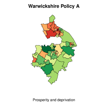
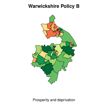
Presently, the decision makers are presented with current and past data concerning relevant issues displayed in graphs and maps within written reports. But these contain no annotated predictions of impact on vulnerable communities of future events or the impact of central government changes in regulation. Nor are evaluations given of the likely effectiveness of different implementations of changes, i.e. policy options. We are currently transferring the output of our analyses to the same types of graphs and maps, but now concerning predictions of the impact of future controls. In Figure 4 we illustrate how their familiar demographic regional map can be used to display ‘hot-spots’ for food riot potential that might occur under certain policies. Here the decision centre can immediately see how a decision is predicted to have a dramatic deleterious effect in the more deprived areas of the region, and because of this, increase the risk of rioting. We have shown that, despite the complexities of the food security system, we have been able to establish the CK-class for this problem, to identify how to make a sound and distributed IDSS using expert judgement based on suitable models, data and elicited domain knowledge, to accommodate rigorously the uncertainty in the information and to provide the SB with an appropriate visualisation of the IDSS outputs to make them usable.
6 Discussion
In this paper we have been able to demonstrate that a formal and feasible IDSS can be designed to enhance a decision centre’s decision-making capabilities. We noted that systems with an underlying clear causal directionality are especially amenable to this type of support. What we usually need is that the functionality of the support to be precisely defined so that a suitable overarching framework can be agreed by all parties - several illustrations of these are given above - and that the IDSS has available sufficient numbers of expert judgements to inform it.
Then it will be possible to continually update the system with the best of the evidence and do this in a distributed way that ensures it remains coherent, sound and feasible. Furthermore, the calculations of scores of policy options will often depend on the expectations of a few functions donated by autonomous panels, communicated to the other panels in simple ways so that uncertainties are appropriately incorporated into the analysis.
Of course, as for any class of statistical model, the validity of the assumptions underpinning its evaluation needs to be checked against both domain knowledge and empirical evidence as this becomes available. As we stated earlier, under the conditions we derive above diagnostic checks of the various component models can be devolved to the responsible panel. But what if the structural assumptions within the CK class appear from data to be violated even though the individual components themselves perform well?
This is a challenging issue and obviously depends critically on both the domain on which the IDSS applies and the nature of the information sets. In crisis management systems like RODOS, as an incident unfolds such structural reappraisal would be very difficult to enact in real time. However, within integrating systems for policy decision support, like the food security system discussed above, such data-driven appraisal and revision may be possible. The obvious way to proceed would be to set the predicted consequences of policy choices made using the system against their predictions. A natural framework for applying these techniques would be the prequential approach (Dawid, 1984) where model predictions of immediate consequences of enacted policies are compared with what was actually observed to happen - for example in terms of comparisons of observed and predicted marginal utility scores - a methodology we plan to fully develop in the future.
Our focus here has been on networking probabilistic models. However this focus was determined mainly because probabilistic decision support tools are the most widely used of those that accommodate uncertainty in some way. We accept there are other modelling tools - for example those based on linear Bayes or belief function inferential schemes - which also have their own formal structures and using similar technologies can also ensure coherent and speedy integrating decision support.
We have noted above that many of the computational forecasting formulae can be expressed algebraically where the systems of equations can be deduced from the elicited overarching system. So, in particular, computer algebra can be used to code up these equations which can then be examined for their algebraic properties. As well as guiding the design of the network architecture of an IDSS, issues like the robustness of the systems to variation in inputs can be formally and systematically analysed using these tools. We have already made some tentative steps in this development (see Leonelli et al., 2015b).
Of course, in some situations the likelihood separation we need to ensure the enduring formal distributivity of a formal IDSS will break down. Then we will need to fall back on approximate inferential methods that preserve distributivity. However preliminary results suggest that sensible approximate methods - whose form is similar to variational Bayes methods - can still work effectively provided that statistical diagnostics are employed to check that the family of models described by the overarching posited structure remains plausible in the light of the information available. These results will be reported in due course.
We believe that, with the increasing demand for complex evidence based models the demand for integrating decision support systems can only increase. If such systems do not encode uncertainty intelligently then as statisticians we know that these will be liable to grossly mislead. But as we demonstrate here it is straightforward to appropriately encode uncertainties into such a framework and in this way to properly appraise the available options.
Acknowledgements
JQS & MJB were funded by EPSRC grant EP/K039628/1, ‘Coherent inference over a network of probabilistic systems for decision support with applications to food security’ and ML was funded by EPSRC grant EP/K007580/1, ‘Management of Nuclear Risk Issues: Environmental, Financial and Safety’, within the NRFES project.
References
- Aguilera et al. (2011) P. A. Aguilera, A. Fernández, R. Fernández, R. Rumí, and A. Salmerón. Bayesian networks in environmental modelling. Envirom. Modell. Softw., 26(12):1376–1388, 2011.
- Anacleto et al. (2013) O. Anacleto, C. M. Queen, and C. J. Albers. Multivariate forecasting of road traffic flows in the presence of heteroscedasticity and measurement errors. J. R. Statist. Soc. C, 62(2):251–270, 2013.
- Barons et al. (2015) M. J. Barons, X. Zhong, and J. Q. Smith. Dynamic Bayesian networks for decision support and sugar food security. Technical Report 14-18, CRISM, The University of Warwick, 2015.
- Best et al. (2005) N. Best, S. Richardson, and A. Thomson. A comparison of Bayesian spatial models for disease mapping. Stat. Methods Med. Res., 14(1):35–59, 2005.
- Bissiri et al. (2013) P. G. Bissiri, C. C. Holmes, and S. G. Walker. A general framework for updating belief distributions. Technical report, arXiv:1306.6430 (to appear in J. R. Statist. Soc. B), 2013.
- Brockwell and Davis (2002) P. J. Brockwell and R. A. Davis. Introduction to time series and forecasting. Springer, New York, 2002.
- Carvalho and West (2007) C. M. Carvalho and M. West. Dynamic matrix-variate graphical models. Bayesian Anal., 2(1):69–97, 2007.
- Conti et al. (2009) S. Conti, J. P. Gosling, J. E. Oakley, and A. O’Hagan. Gaussian process emulation of dynamic computer codes. Biometrika, 96(3):663–676, 2009.
- Cooper and Yoo (1999) G. F. Cooper and C. Yoo. Causal discovery from a mixture of experimental and observational data. In Proceedings of the 15th Conference on Uncertainty in Artificial Intelligence, pages 116–125, 1999.
- Costa et al. (2015) L. Costa, J. Q. Smith, T. Nichols, J. Cussens, E. P. Duff, and T. R. Makin. Searching multiregression dynamic models of resting-state fMRI networks using integer programming. Bayesian Anal., 10(2):441 – 478, 2015.
- Cowell and Smith (2014) R. G. Cowell and J. Q. Smith. Causal discovery through MAP selection of stratified chain event graphs. Electron. J. Stat., 8(1):965–997, 2014.
- Cowell et al. (1999) R. G. Cowell, P. Dawid, S. L. Lauritzen, and D. J. Spiegelhalter. Probabilistic networks and expert systems. Springer, New York, 1999.
- Cowell et al. (2011) R. G. Cowell, S. L. Lauritzen, and J. Mortera. Probabilistic expert systems for handling artifacts in complex DNA mixtures. Forensic Sci. Int., 5(3):202–209, 2011.
- Daneshkhah and Smith (2004) A. Daneshkhah and J. Q. Smith. Hypercausality, randomisation, and local and global independence. In Advances in Bayesian Networks, pages 1–18. 2004.
- Darmon et al. (2004) N. Darmon, A. Briend, and A. Drewnowski. Energy-dense diets are associated with lower diet costs: a community study of french adults. Public Health Nutr., 7(1):21–27, 2004.
- Darmon et al. (2014) N. Darmon, A. Lacroix, L. Muller, and B. Ruffieux. Food price policies improve diet quality while increasing socioeconomic inequalities in nutrition. Int. J. Behav. Nutr. Phy., 11:66, 2014.
- Dawid (1984) A. P. Dawid. Present position and potential developments: some personal views. Statistical theory: the prequential approach. J. R. Stat. Soc. A, 147(2):278–292, 1984.
- Dawid (2001) A. P. Dawid. Separoids: a mathematical framework for conditional independence and irrelevance. Ann. Math. Artif. Intel., 32(1-4):335–372, 2001.
- Dawid (2002) A. P. Dawid. Influence diagrams for causal modelling and inference. Int. Stat. Rev., 70(2):161–189, 2002.
- Dawid and Didelez (2010) A. P. Dawid and V. Didelez. Identifying the consequences of dynamic treatment strategies: a decision-theoretic overview. Stat. Surv., 4:184–231, 2010.
- Dawid and Lauritzen (1993) A. P. Dawid and S. L. Lauritzen. Hyper Markov laws in the statistical analysis of decomposable graphical models. Ann. Stat., 21(3):1272–1317, 1993.
- Dawid et al. (2007) A. P. Dawid, J. Mortera, and P. Vicard. Object-oriented Bayesian networks for complex forensic DNA profiling problems. Forensic. Sci. Int., 169(2):195–205, 2007.
- De and Faria (2011) S. De and Á. E. Faria. Dynamic spatial Bayesian models for radioactivity deposition. J. Time Ser. Anal., 32(6):607–617, 2011.
- Decuyper et al. (2014) A. Decuyper, A. Rutherford, A. Wadhwa, J. M. Bauer, G. Krings, T. Gutierrez, V. D. Blondel, and M. A. Luengo-Oroz. Estimating food consumption and poverty indices with mobile phone data. Technical report, arXiv:1412.2595v1, 2014.
- DEFRA (2009) DEFRA. UK food security assessment: detailed analysis. Technical report, Department for Environment, Food and Rural Affairs, 2009.
- Dodd and Smith (2012) L. Dodd and J. Q. Smith. Devolving command decisions in complex operations. J. Oper. Res. Soc., 64(1):17–33, 2012.
- Donkin et al. (1999) A. J. M. Donkin, E. A. Dowler, S. J. Stevenson, and S. A. Turner. Mapping access to food at a local level. Brit. Food J., 101(7):554–564, 1999.
- Dowler (2010) E. A. Dowler. Income needed to achieve a minimum standard of living. BMJ, 341:c4070, 2010.
- Dowler (2014) E. A. Dowler. Comments from Professor Elizabeth Dowler on Feeding Britain: a Strategy for zero hunger in England, Wales, Scotland and Northern Ireland, 2014.
- Dowler et al. (2001) E. A. Dowler, S. A. Turner, and B. Dobson. Poverty bites: food, health and poor families. Poverty publication. Child Poverty Action Group, Great Britian, 2001.
- Drewnowski and Specter (2004) A. Drewnowski and S. E. Specter. Poverty and obesity: the role of energy density and energy costs. Am. J. Clin. Nutr., 79(1):6–16, 2004.
- Economist (2015) Economist. Global food security index. Web, 2015. URL http://foodsecurityindex.eiu.com/.
- Efendigil et al. (2009) T. Efendigil, S. Önüt, and C. Kahraman. A decision support system for demand forecasting with artificial neural networks and neuro-fuzzy models: a comparative analysis. Expert Syst. Appl., 36(3):6697 – 6707, 2009.
- Ehrhardt (1997) J. Ehrhardt. The RODOS system: decision support for off-site emergency management in Europe. Radiat. Prot. Dosim., 73(1):35–40, 1997.
- Ehrhardt et al. (1993) J. Ehrhardt, J. Pasler-Sauer, O. Schule, G. Benz, M. Rafat, and J. Richter. Development of RODOS, a comprehensive decision support system for nuclear emergencies in Europe - an overview. Radiat. Prot. Dosim., 50(2-4):195–203, 1993.
- Eichler and Didelez (2007) M. Eichler and V. Didelez. Causal reasoning in graphical time series models. In Proceedings of the 23rd Conference on Uncertainty in Artifical Intelligence, pages 109–116, 2007.
- Elia et al. (2010) M. Elia, C. A. Russell, and R. J. Stratton. Malnutrition in the UK: policies to address the problem. P. Nutr. Soc., 69:470–476, 2010.
- Elliott (2014) C. Elliott. Elliott review into the integrity and assurance of food supply networks - final report. A national food crime prevention framework. Technical report, H. M. Government, 2014.
- Faria and Smith (1997) Á. E. Faria and J. Q. Smith. Conditionally externally Bayesian pooling operators in chain graphs. Ann. Stat., 25(4):1740–1761, 1997.
- Field et al. (2014) F. Field, T. Thornton, J. Glen, B. Jenkin, E. Lewell-Buck, and S. Newton. Feeding Britain: a strategy for zero hunger in England, Wales, Scotland and Northern Ireland. Technical report, All-Party Parliamentary Inquiry into Hunger in the United Kingdom, 2014.
- Freeman and Smith (2011) G. Freeman and J. Q. Smith. Dynamic staged trees for discrete multivariate time series: forecasting, model selection and causal analysis. Bayesian Anal., 6(2):279–305, 2011.
- French (1995) S. French. Uncertainty and imprecision: modelling and analysis. J. Oper. Res. Soc., 46(1):70–79, 1995.
- French (2011) S. French. Aggregating expert judgement. Rev. Real Acad. Cienc., 105(1):181–206, 2011.
- French et al. (1991) S. French, R. M. Cooke, and F. Vogt. The use of expert judgement in the context of a physical model. In Bayesian Statistics IV, pages 617–624, 1991.
- French et al. (2009) S. French, J. Maule, and K. N. Papamichail. Decision behaviour, analysis and support. Cambridge University Press, Cambridge, 2009.
- Friel and Conlon (2004) S. Friel and C. Conlon. Food Poverty and Policy. Combat Poverty Agency, 2004.
- Frydenberg (1990) M. Frydenberg. The chain graph Markov property. Scand. J. Stat., 17:333–353, 1990.
- Goldstein and O’Hagan (1996) M. Goldstein and A. O’Hagan. Bayes linear sufficiency and systems of expert posterior assessments. J. R. Statist. Soc. B, 58(2):301–316, 1996.
- Gómez (2004) M. Gómez. Real-world applications of influence diagrams. In Advances in Bayesian networks, pages 161–180. Springer, 2004.
- Hernandez and Bennison (2000) T. Hernandez and D. Bennison. The art and science of retail location decisions. Int. J. Retail. Distrib. Manag., 28(8):357–367, 2000.
- Higgins and Green (2008) J. P. T. Higgins and S. Green. Cochrane handbook for systematic reviews of interventions. Wiley Online Library, 2008.
- Holmes (2008) B. Holmes. The influence of food security and other social and environmental factors on diet in the national low income diet and nutrition survey. P. Nutr. Soc., 67(OCE):E88, 5 2008.
- Jewell et al. (2009) C. P. Jewell, T. Kypraios, P. Neal, and G. O. Roberts. Bayesian analysis for emerging infectious diseases. Bayesian Anal., 4(3):465–496, 2009.
- Jirousek and Vejnarova (2003) R. Jirousek and J. Vejnarova. Construction of multidimensional models by operators of composition: current state of art. Soft Comput., 7(5):328–335, 2003.
- Johnson and Mengersen (2012) S. Johnson and K. Mengersen. Integrated Bayesian network framework for modeling complex ecological issues. Integrat. Environ. Assess. Manag., 8(3):480–490, 2012.
- Johnson et al. (2014) S. Johnson, E. Abal, K. Ahern, and G. Hamilton. From science to management: using Bayesian networks to learn about Lyngbya. Stat. Sci., 29(1):36–41, 2014.
- Joyce et al. (2014) R. Joyce, K. C. Arikatla, L. O’Connor, and A. Walvis. Totally addicted to space: overcapacity in UK grocery still needs to be addressed. Technical report, Goldman Sachs, 2014.
- Keeney and Raiffa (1993) R. L. Keeney and H. Raiffa. Decision with multiple objectives: preferences and value trade-offs. Cambridge University Press, Cambridge, 1993.
- Kennedy and O’Hagan (2001) M. C. Kennedy and A. O’Hagan. Bayesian calibration of computer models. J. R. Statist. Soc. B, 63(3):425–464, 2001.
- Koller and Lerner (2001) D. Koller and U. Lerner. Sampling in factored dynamic systems. In Sequential Monte Carlo Methods in Practice, pages 445–464. Springer-Verlag, 2001.
- Koller and Pfeffer (1997) D. Koller and A. Pfeffer. Object-oriented Bayesian networks. In Proceedings of the 13th Conference on Uncertainty in Artificial Intelligence, pages 302–313, 1997.
- Kuo et al. (2002) R. J. Kuo, S. C. Chi, and S. S. Kao. A decision support system for selecting convenience store location through integration of fuzzy AHP and artificial neural network. Comput. Ind., 47(2):199–214, 2002.
- Lagi et al. (2012) M. Lagi, Y. Bar-Yam, and Y. Bar-Yam. The food crises: the US drought. Technical report, arXiv:1209.6376, 2012.
- Lagi et al. (2012a) M. Lagi, Y. Bar-Yam, K. Z. Bertrand, and Y. Bar-Yam. The food crises: a quantitative model of food prices including speculators and ethanol conversion. Technical report, arXiv:1203.1313, 2012a.
- Lambie-Mumford and Dowler (2015) H. Lambie-Mumford and E. Dowler. Hunger, food charity and social policy - challenges faced by the emerging evidence base. Soc. Pol. Soc., 14(3):1–10, 2015.
- Lambie-Mumford and Dowler (2014) H. Lambie-Mumford and E. A. Dowler. Rising use of “food aid” in the United Kingdom. Brit. Food J., 116(9):1418–1425, 2014.
- Lauritzen (1992) S. L. Lauritzen. Propagation of probabilities, means and variances in mixed graphical association models. J. Am. Stat. Assoc., 87(420):1098–1108, 1992.
- Lauritzen (1996) S. L. Lauritzen. Graphical models. Oxford University Press, Oxford, 1996.
- Lauritzen and Richardson (2002) S. L. Lauritzen and T. S. Richardson. Chain graph models and their causal interpretations. J. R. Statist. Soc. B, 64(3):321–348, 2002.
- Leonelli (2015) M. Leonelli. Bayesian decision support in complex modular systems: an algebraic and graphical approach. PhD thesis, University of Warwick, 2015.
- Leonelli and Smith (2013) M. Leonelli and J. Q. Smith. Using graphical models and multi-attribute utility theory for probabilistic uncertainty handling in large systems, with application to the nuclear emergency management. In 29th International Conference on Data Engineering Workshops (ICDEW), pages 181–192, 2013.
- Leonelli and Smith (2015) M. Leonelli and J. Q. Smith. Bayesian decision support for complex systems with many distributed experts. Ann. Oper. Res., 235(1):517–542, 2015.
- Leonelli et al. (2015a) M. Leonelli, E. Riccomagno, and J. Q. Smith. The algebra of integrated partial belief systems. Technical Report 15-08, CRISM, The University of Warwick, 2015a.
- Leonelli et al. (2015b) M. Leonelli, E. Riccomagno, and J. Q. Smith. Using computer algebra to symbolically evaluate discrete influence diagrams. Technical Report 15-07, CRISM, The University of Warwick, 2015b.
- Loopstra and Tarasuk (2012) R. Loopstra and V. Tarasuk. The relationship between food banks and household food insecurity among low-income Toronto families. Can. Public Pol., 38:497–514, 2012.
- Loopstra et al. (2015) R. Loopstra, A. Reeves, D. Taylor-Robinson, B. Barr, M. McKee, and D. Stuckler. Austerity, sanctions, and the rise of food banks in the UK. BMJ, 350, 2015.
- Mahoney and Laskey (1996) S. M. Mahoney and K. B. Laskey. Network engineering for complex belief networks. In Proceedings of the 12th Conference on Uncertainty in Artificial Intelligence, pages 389–396, 1996.
- Massa and Lauritzen (2010) M. S. Massa and S. L. Lauritzen. Combining statistical models. Contemp. Math., 516:239–259, 2010.
- McBride and Purcell (2014) K. McBride and S. Purcell. Food, fuel, finance tackling the poverty premium. Technical report, Church Action on Poverty, 2014.
- McKinley et al. (2014) T. J. McKinley, J. V. Ross, R. Deardon, and A. R. Cook. Simulation-based Bayesian inference for epidemic models. Comput. Stat. Data An., 71:434–447, 2014.
- Molina et al. (2010) J. L. Molina, J. Bromley, J. L. García-Aróstegui, C. Sullivan, and J. Benavente. Integrated water resources management of overexploited hydrogeological systems using object-oriented Bayesian networks. Envirom. Modell. Softw., 25(4):383–397, 2010.
- Morris et al. (2000) J. N. Morris, A. J. M. Donkin, D. Wonderling, P. Wilkinson, and E. A. Dowler. A minimum income for healthy living. J. Epidemiol. Commun. H., 54(12):885–889, 2000.
- Murphy (2002) K. P. Murphy. Dynamic Bayesian networks: representation, inference and learning. PhD thesis, University of California, Berkeley, 2002.
- Nicholson and Flores (2011) A. E. Nicholson and M. J. Flores. Combining state and transition models with dynamic Bayesian networks. Ecol. Model., 222(3):555–566, 2011.
- Nilsson (2001) D. Nilsson. The computation of moments of decomposable functions in probabilistic expert systems. In Proceedings of the 3rd International Symposium on Adaptive Systems, pages 116–121, 2001.
- O’Hagan et al. (2006) A. O’Hagan, C. E. Buck, A. Daneshkhah, J. R. Eiser, P. H. Garthwaite, D. J. Jenkinson, J. E. Oakley, and T. Rakow. Uncertain judgements: eliciting experts’ probabilities. John Wiley & Sons, Chichester, 2006.
- ONS (2013) ONS. Consumer price indices: a brief guide. Technical report, Office for National Statistics, 2013.
- Papamichail and French (2003) K. N. Papamichail and S. French. Explaining and justifying the advice of a decision support system: a natural language generation approach. Expert Syst. Appl., 24(1):35–48, 2003.
- Papamichail and French (2005) K. N. Papamichail and S. French. Design and evaluation of an intelligent decision support system for nuclear emergencies. Decis. Support Syst., 41(1):84–111, 2005.
- Papamichail and French (2013) K. N. Papamichail and S. French. 25 Years of MCDA in nuclear emergency management. IMA J. Manag. Math., 24(4):481–503, 2013.
- Pearl (1988) J. Pearl. Probabilistic reasoning in intelligent systems: networks of plausible inference. Morgan Kaufmann, San Francisco, 1988.
- Pearl (2000) J. Pearl. Causality: models, reasoning and inference. Cambridge University Press, Cambridge, 2000.
- Peterson (2009) M. Peterson. An introduction to decision theory. Cambridge University Press, Cambridge, 2009.
- Pilgrim et al. (2012) A. Pilgrim, M. Barker, A. Jackson, G. Ntani, S. Crozier, H. Inskip, K. Godfrey, C. Cooper, and S. Robinson. Does living in a food insecure household impact on the diets and body composition of young children? Findings from the Southampton Women’s Survey. J. Epidemiol. Commun. H., 66(6):e6, 2012.
- Queen (1994) C. M. Queen. Using the multiregression dynamic model to forecast brand sales in a competitive product market. The Statistician, 43(1):87–98, 1994.
- Queen and Albers (2009) C. M. Queen and C. J. Albers. Intervention and causality: forecasting traffic flows using a dynamic Bayesian network. J. Am. Stat. Assoc., 104(486):669–681, 2009.
- Queen and Smith (1993) C. M. Queen and J. Q. Smith. Multiregression dynamic models. J. R. Statist. Soc. B, 55(4):849–870, 1993.
- Queen et al. (2008) C. M. Queen, B. J. Wright, and C. J. Albers. Forecast covariances in the linear multiregression dynamic model. J. Forecasting, 27(2):175–191, 2008.
- Riccomagno and Smith (2004) E. Riccomagno and J. Q. Smith. Identifying a cause in models which are not simple Bayesian networks. In Proceedings of the 10th Conference on Information Processing and Management of Uncertainty in Knowledge-Based Systems, pages 1315–1322, 2004.
- Richter et al. (2002) K. Richter, F. Gering, and H. Müller. Data assimilation for assessing radioactive contamination of feed and foodstuffs. In Development and Application of Computer techniques to Environmental Studies, pages 393–402. WIT Press, 2002.
- Sansó et al. (2008) B. Sansó, C. E. Forest, and D. Zantedeschi. Inferring climate system properties using a computer model. Bayesian Anal., 3(1):1–37, 2008.
- Shafer (1976) G. R. Shafer. A mathematical theory of evidence. Princeton University Press, Princeton, 1976.
- Shafer (1996) G. R. Shafer. The Art of Causal Conjecture. MIT Press, Cambridge, 1996.
- Shpitser and Pearl (2008) I. Shpitser and J. Pearl. Complete identification methods for the causal hierarchy. J. Mach. Learn. Res., 9:1941–1979, 2008.
- Smets (2005) P. Smets. Decision making in the TBM: the necessity of the pignistic transformation. Int. J. Approx. Reason., 38(2):133–147, 2005.
- Smith (1989) J. Q. Smith. Influence diagrams for Bayesian decision analysis. Eur. J. Oper. Res., 40(3):363–376, 1989.
- Smith (1996) J. Q. Smith. Plausible Bayesian games. In Bayesian Statistics 5, pages 387–406. 1996.
- Smith (2010) J. Q. Smith. Bayesian decision analysis: principles and practice. Cambridge University Press, Cambridge, 2010.
- Smith and Anderson (2008) J. Q. Smith and P. E. Anderson. Conditional independence and chain event graphs. Artif. Intell., 172(1):42–68, 2008.
- Smith and Dodd (2012) J. Q. Smith and L. Dodd. Regulating autonomous agents facing conflicting objectives: a command and control example. Decis. Anal., 9(2):165–171, 2012.
- Smith and Figueroa (2007) J. Q. Smith and L. J. Figueroa. A causal algebra for dynamic flow networks. In Advances in Probabilistic Graphical Models, pages 39–54, 2007.
- Smith and Papamichail (1999) J. Q. Smith and K. N. Papamichail. Fast Bayes and the dynamic junction forest. Artif. Intell., 107(1):99–124, 1999.
- Smith et al. (1997) J. Q. Smith, Á. E. Faria, S. French, D. Ranyard, D. Vlesshhouwer, J. Bohunova, T. Duranova, M. Stubna, L. Dutton, C. Rojas, and A. Sohier. Probabilistic data assimilation within RODOS. Radiat. Prot. Dosim., 73(1):57–59, 1997.
- Spiegelhalter and Lauritzen (1990) D. J. Spiegelhalter and S. L. Lauritzen. Sequential updating of conditional probabilities on directed graphical structures. Networks, 20(5):579–605, 1990.
- Spirtes et al. (1993) P. Spirtes, C. Glymour, and R. Scheines. Causation, prediction, and search. MIT Press, Cambridge, 1993.
- Studeny (2006) M. Studeny. Probabilistic conditional independence structures. Springer, London, 2006.
- Thwaites et al. (2010) P. A. Thwaites, J. Q. Smith, and E. Riccomagno. Causal analysis with chain event graphs. Artif. Intell., 174(12-13):889–909, 2010.
- USDA (2012) Economic Research Service USDA. U.S. household food security survey module. Technical report, Economic Research Service, USDA, 2012.
- Walle and Turoff (2008) B. Walle and M. Turoff. Decision support for emergency situations. Inf. Syst. E-Bus. Manage., 6(3):295–316, 2008.
- Wermuth and Lauritzen (1990) N. Wermuth and S. L. Lauritzen. On substantive research hypotheses, conditional independence graphs and graphical chain models. J. R. Statist. Soc. B, 52(1):21–50, 1990.
- West and Harrison (1997) M. West and P. J. Harrison. Bayesian forecasting and dynamic models. Springer, New York, 1997.
- Williamson and Goldstein (2011) D. Williamson and M. Goldstein. Bayesian policy support for adaptive strategies using computer models for complex physical systems. J. Oper. Res. Soc., 63(8):1021–1033, 2011.
- Williamson et al. (2012) D. Williamson, M. Goldstein, and A. Blaker. Fast linked analyses for scenario-based hierarchies. J. R. Statist. Soc. C, 61(5):665–691, 2012.
- Xiang (2002) Y. Xiang. Probabilistic reasoning in multiagent systems. Cambridge University Press, Cambridge, 2002.
- Zheng et al. (2009) D. Q. Zheng, J. K. C. Leung, and B. Y. Lee. Online update of model state and parameters of a Monte Carlo atmospheric dispersion model by using ensemble Kalman filter. Atmos. Environ., 43(12):2005–2011, 2009.
7 Appendix
7.1 Proof of Theorem 3.1
Fix a and for simplicity suppress this dependence and the time index . We need show that under the conditions of the theorem at any time and under any policy the SB will continue to hold panel independent beliefs, i.e. that, for ,
| (7.1) |
and that when assessing , she will only use the information would use if acting autonomously in assessing the information she needs to deliver, i.e. that
| (7.2) |
This is then sufficient for soundness and distributivity. Because even if all panellists could share each other’s information then, given all panel beliefs, they would come to the same assessment about the joint distribution of the relevant parameters: that all panel subvectors are mutually independent of each other and that these margins will simply be the margins of the associated panel were they making decisions autonomously.
The proof simply uses the semi-graphoid axioms of conditional independence as stated in Smith (1989):
Symmetry: For any three vectors of measurements,
Perfect composition: For any four disjoint vectors of measurements,
We start by proving the panel independence condition in (7.1). Note that from common separability in equation (3.4) it follows that
| which combined with the separately informed condition in equation (3.2) through perfect decomposition and using the symmetric property of semi-graphoids axioms gives | ||||
| Using again perfect decomposition and symmetry, it follows that | ||||
| (7.3) | ||||
| Now the cutting condition in equation (3.3) together with equation (7.3) implies by perfect decomposition that | ||||
| (7.4) | ||||
| Then again by perfect decomposition we have that | ||||
| Since is a function of the above expression is equivalent to | ||||
| (7.5) | ||||
| The delegatable condition in equation (3.1) can be written as | ||||
| so, using perfect decomposition, it follows that | ||||
| (7.6) | ||||
| Combining via perfect decomposition equations (7.5) and (7.6) and using the symmetry property we have that | ||||
| So using again perfect decomposition it follows that | ||||
which, since and are functions of , can be written as equation (7.1). This shows that panel independence directly follows from the four conditions of Definition 3.2.
To show that equation (7.2) holds, note that another implication of delegatability in equation (3.1) by perfect decomposition is that
| (7.7) | ||||
| where again we used the fact that is a function of . Now noting that by perfect decomposition equation (7.4) implies that | ||||
| (7.8) | ||||
| it follows from equations (7.7) and (7.8) by perfect decomposition that | ||||
which, since is a function of is equivalent to equation (7.2).
7.2 Proof of Theorem 3.2
Fix a policy and suppress for ease of notation this dependence. Under the initial hypotheses, by Theorem 3.1
implying that the prior joint density can be written in a product form
| It follows that under this admissibility protocol | ||||
| where from the form of the likelihood above | ||||
By hypothesis will be delivered by and adopted by the SB. So the IDSS is sound. In particular we can deduce, through the definition of panel separability and the results of Theorem 3.1, that
So we have separability a posteriori. Note that in the notation above
and, for ,
Since by definition is known to , , the system is also delegatable. Finally note that if
on a set of non zero prior measure, then the conditional density on will have the property that for all
where denotes the density delivered by panel for the parameters it oversees in . This means that panel parameters are a posteriori dependent and so in particular the density determined by the margins is not sound.