Multiple Extended Target Tracking with Labelled Random Finite Sets

Abstract

Targets that generate multiple measurements at a given instant in time are commonly known as extended targets. These present a challenge for many tracking algorithms, as they violate one of the key assumptions of the standard measurement model. In this paper, a new algorithm is proposed for tracking multiple extended targets in clutter, that is capable of estimating the number of targets, as well the trajectories of their states, comprising the kinematics, measurement rates and extents. The proposed technique is based on modelling the multi-target state as a generalised labelled multi-Bernoulli (GLMB) random finite set (RFS), within which the extended targets are modelled using gamma Gaussian inverse Wishart (GGIW) distributions. A cheaper variant of the algorithm is also proposed, based on the labelled multi-Bernoulli (LMB) filter. The proposed GLMB/LMB-based algorithms are compared with an extended target version of the cardinalised probability hypothesis density (CPHD) filter, and simulation results show that the (G)LMB has improved estimation and tracking performance.

I Introduction

Multi-target tracking is the process of estimating the number of targets and their states, based upon imperfect sensor measurements that are typically corrupted by noise, missed detections, and false alarms. The main challenge is to filter out these three effects in order to gain accurate estimates of the true target states. A Bayesian approach to this type of problem requires models to describe how the measurements are related to the underlying target states. Most traditional trackers use the so-called standard measurement model. This is also known as a point target model, since it is based on the assumption that each target produces at most one measurement at a given time, and that each measurement originates from at most one target. This model simplifies the development of multi-target trackers, but in practice it is often an unrealistic representation of the true measurement process.

More realistic measurement processes can be handled using more sophisticated non-standard measurement models, which may relax the aforementioned assumptions, usually at the expense of increased computation. One example of this is when a group of targets produces a single measurement, known as an unresolved target (or merged measurement) model [1]. This model is useful when dealing with low-resolution sensors that cannot generate seperate detections for closely spaced targets. On the other hand, higher resolution sensors may produce multiple measurements per target on any given scan. Such cases require the use of an extended target model [2], which is the subject of this paper.

Extended target measurement models typically require two components; a model for the number of measurements generated by each target, and a model for their spatial distribution. These depend strongly on both the sensor characteristics and the type of targets being tracked. For example, in radar tracking, some targets may generate many separate detections, by virtue of the fact that they possess many scatter points. However, other targets may reflect most of the energy away from the receiver, leading to very few detections, or none at all. In general, when a target is far enough away from the sensor, its detections can often be characterised as a cluster of points exhibiting no discernable geometric structure. In such cases, the number of measurements is usually modelled using a Poisson distribution, see for example [2] and [3].

Even in the absence of a specific target structure, it is still possible to estimate the size and shape of a target, known as the target extent. This can be achieved by assuming some general parameteric shape for the extent, for which the parameters are estimated based on the spatial arrangement of the observations. An approach that assumes an elliptical extent was proposed in [4], which used a multivariate Gaussian, parameterised by a random covariance matrix with an inverse Wishart distribution. This was termed a Gaussian inverse Wishart (GIW), and this method enables the target extent to be estimated on-line, instead of requiring prior specification. Further applications and improvements have appeared in [5, 6, 7]. Alternative methods for estimating target extent have also been proposed, see for example [8, 9, 10].

The GIW method has been applied using multi-target filters based on the random finite set (RFS) framework. A probability hypothesis density (PHD) filter, which was originally developed by Mahler in [11] for the point target model, was proposed for extended multi-target filtering in [12]. An implementation of this filter based on the GIW model (GIW-PHD filter) was developed in [13]. The cardinalised PHD (CPHD) filter [27] is a generalisation of the PHD filter, which models the multi-target state as an i.i.d cluster RFS instead of a Poisson RFS. This was applied to extended targets in [14], which also incorporated a modification to the GIW approach [15], enabling the estimation of target measurement rates. This method treats the rate parameter of the Poisson pdf (which characterises the number of measurements generated by a target) as a random variable, whose distribution is modelled as a gamma pdf. This algorithm was called the gamma Gaussian inverse Wishart CPHD (GGIW-CPHD) filter. Extended target PHD and CPHD filters have also been presented in [32, 33].

The advantage of the (C)PHD filters is that they reduce the computational cost of the Bayes multi-target filter, but to do so, some significant approximations are made. While these approximations avoid explicit data association, it means that the filters do not produce target tracks, and the PHD filter can produce highly uncertain estimates of the target number due to the Poisson cardinality assumption [11, 18]. Another limitation affecting the CPHD filter is the so-called ‘spooky’ effect [19], which means a target misdetection may cause a false estimate to spontaneously appear in a different part of the state space. A Bernoulli filter for extended targets was proposed in [20], which does not suffer from these issues, however, it is limited to at most a single target in clutter.

A recently proposed algorithm that addresses these limitations is called the generalised labelled multi-Bernoulli (GLMB) filter [21, 22]. This algorithm has been shown to outperform both the PHD and CPHD filters, with the added advantage of producing labelled track estimates, albeit with a higher computational cost. An approximate but computationally cheaper version of this filter was proposed in [23], called the labelled multi-Bernoulli filter (LMB). Also, the first GLMB filter for a non-standard measurement model was developed in [1], which used a model that includes merged measurements, a problem which can be viewed as the dual of the extended target tracking problem.

In this paper, we develop a GLMB filter for extended multi-target tracking based on the GGIW model. The resulting algorithm (GGIW-GLMB) is capable of estimating the kinematics and extents of multiple extended targets in clutter, with the advantage of producing full target tracks. Preliminary results on this work have been presented in [24], which we build upon in the following ways. Firstly, we provide a complete derivation of the extended target likelihood function used by the filter. Second, we have implemented and tested a computationally cheaper version of the algorithm, called the GGIW labelled multi-Bernoulli (GGIW-LMB) filter. Third, we have improved the utility of the filter by incorporating an adaptive target birth model, allowing new targets to appear from anywhere in the state space. Finally, we have applied the algorithms to a real-world data set obtained from a lidar sensor used in autonomous vehicle applications.

The paper is organised as follows. Section II contains a brief background on the GLMB, and in Section III we adapt it to extended multi-target tracking, by proposing an extended target likelihood and deriving the associated GGIW-GLMB and GGIW-LMB filters. Section IV presents details relating to the implementation of these algorithms. Section V contains simulation results comparing the performance of the GGIW-(G)LMB with the GGIW-CPHD filter, and in Section VI we demonstrate an application to real-world measurement data. Finally, we make some concluding remarks in Section VII.

II Background: Tracking with Labelled Random Finite Sets

The essence of the RFS approach to multi-target tracking is the modelling of the multi-target states and measurements as finite set-valued random variables, or RFSs. Until recently, estimation algorithms derived using this framework have been based on the use of unlabelled random finite sets, as demonstrated by the PHD [11], CPHD [27] and multi-target multi-Bernoulli (MeMBer) [28] filters. A key reason for the popularity of these approaches is that they do not require explicit data association. However, their main disadvantage is that they only provide sets of unlabelled point estimates at each time step, so in applications that require target trajectories, tracks must be formed via additional post-processing. To address this problem, the concept of labelled random finite sets was proposed [21], which involves assigning a distinct label to each target, such that each target’s trajectory can be identified without the need for post-processing.

In [21], a class of labelled RFS called generalised labelled multi-Bernoulli (GLMB) was proposed, and based on this formulation, an algorithm for solving the multi-target tracking problem under the standard point-target likelihood model was developed. In the remainder of this section we briefly review some of the key points of this technique, and in Section III we adapt this method to tracking multiple extended targets.

We begin by introducing some notation and definitions relating to labelled random finite sets. The multi-object exponential of a real valued function $h$ raised to a set $X$ is defined as $\left[h\left(\cdot\right)\right]^{X}=\prod_{x\in X}h\left(x\right)$, where $h^{\emptyset}=1$, and the elements of $X$ may be of any type such as scalars, vectors, or sets, provided that the function $h(\cdot)$ takes an argument of that type. The generalised Kronecker delta function, and the set inclusion function are respectively defined as

$$\delta_{Y}\left(X\right)=\begin{cases}1,&\mbox{ if }X=Y\\ 0,&\mbox{ otherwise}\end{cases},\quad 1_{Y}\left(X\right)=\begin{cases}1,&\text{if }X\subseteq Y\\ 0,&\text{otherwise}\end{cases},$$

where again, $X$ and $Y$ may be of any type, such as scalars, vectors, or sets. In general, we adopt the notational convention that labelled sets are expressed in bold upper case ($\boldsymbol{X}$), unlabelled sets in regular upper case ($X$), labelled vectors in bold lower case ($\boldsymbol{x}$), and unlabelled vectors or scalars in regular lower case ($x$).

Definition 1.

A labelled RFS $\boldsymbol{X}$ with state space $\mathbb{X}$ and discrete label space $\mathbb{L}$, is an RFS on $\mathbb{X}\times\mathbb{L}$, such that the labels within each realisation are always distinct. That is, if $\mathcal{L\left(\boldsymbol{X}\right)}$ is the set of unique labels in $\boldsymbol{X}$, and we define the distinct label indicator function as

$$\Delta\left(\boldsymbol{X}\right)=\begin{cases}1,&\mbox{if }\left|\mathcal{L}\left(\boldsymbol{X}\right)\right|=\left|\boldsymbol{X}\right|\\ 0,&\mbox{if }\left|\mathcal{L}\left(\boldsymbol{X}\right)\right|\neq\left|\boldsymbol{X}\right|\end{cases}$$ (1)

then a labelled RFS $\boldsymbol{X}$ always satisfies $\Delta\left(\boldsymbol{X}\right)=1$.

Definition 2.

A labelled multi-Bernoulli (LMB) RFS is a labelled RFS with state space $\mathbb{X}$ and discrete label space $\mathbb{L}$, which is distributed according to

$$\boldsymbol{\pi}\left(\boldsymbol{X}\right)=\Delta\left(\boldsymbol{X}\right)w\left(\mathcal{L}\left(\boldsymbol{X}\right)\right)\left[p\left(\cdot\right)\right]^{\boldsymbol{X}},$$ (2)

where

$$w\left(L\right) =\prod_{i\in\mathbb{L}}\left(1-r^{\left(i\right)}\right)\prod_{l\in L}\frac{1_{L}\left(l\right)r^{\left(l\right)}}{1-r^{\left(l\right)}},$$ (3)

$$p\left(x,l\right) =p^{\left(l\right)}\left(x\right),$$ (4)

in which $r^{\left(l\right)}$ and $p^{\left(l\right)}\left(\cdot\right)$ are the existence probability and probability density corresponding to label $l\in\mathbb{L}$. An LMB distribution is abbreviated using the notation $\boldsymbol{\pi}\left(\boldsymbol{X}\right)=\left\{\left(r^{\left(l\right)},p^{\left(l\right)}\right)\right\}_{l\in\mathbb{L}}$.

Definition 3.

A generalised labelled multi-Bernoulli (GLMB) RFS is a labelled RFS with state space $\mathbb{X}$ and discrete label space $\mathbb{L}$, which is distributed according to

$$\boldsymbol{\pi}\left(\boldsymbol{X}\right)=\Delta\left(\boldsymbol{X}\right)\sum\limits_{c\in\mathbb{C}}w^{\left(c\right)}\left(\mathcal{L}\left(\boldsymbol{X}\right)\right)\left[p^{\left(c\right)}\left(\cdot\right)\right]^{\boldsymbol{X}},$$ (5)

where $\mathbb{C}$ is a discrete index set, and $w^{\left(c\right)}\left(L\right)$ and $p^{\left(c\right)}\left(x,l\right)$ satisfy

$$\sum_{L\subseteq\mathbb{L}}\sum\limits_{c\in\mathbb{C}}w^{\left(c\right)}\left(L\right)=1,\quad\int_{x\in\mathbb{X}}p^{\left(c\right)}\left(x,l\right)dx=1.$$ (6)

In Bayesian multi-target tracking, the goal at time $k$ is to estimate a finite set of labelled states $\boldsymbol{X}_{k}\subset\mathbb{X}\times\mathbb{L}$, called the multi-target state, based on finite sets of incoming multi-target observations $Z_{k}\subset\mathbb{Z}$. We model $\boldsymbol{X}_{k}$ as a labelled random finite set, and $Z_{k}$ as an unlabelled random finite set. A principled mathematical framework for working with RFSs is called finite set statistics (FISST) [25], the cornerstone of which is a notion of multi-target density/integration that is consistent with point process theory [26].

The multi-target state at each time $k$ is distributed according to a multi-target density $\boldsymbol{\pi}_{k}\left(\cdot|Z_{1:k}\right)$, where $Z_{1:k}$ is an array of finite sets of measurements received up to time $k$. The multi-target density is recursively propagated in time via a multi-target prediction and update as follows.

The multi-target prediction to time $k$ is given by the Chapman-Kolmogorov equation

$$\boldsymbol{\pi}_{k|k-1}\left(\boldsymbol{X}_{k}|Z_{1:k-1}\right)$$ (7)

$$\qquad=\int f_{k|k-1}\left(\boldsymbol{X}_{k}|\boldsymbol{X}\right)\boldsymbol{\pi}_{k-1}\left(\boldsymbol{X}|Z_{1:k-1}\right)\delta\boldsymbol{X},$$

where $f_{k|k-1}\left(\boldsymbol{X}_{k}|\boldsymbol{X}\right)$ is the multi-target transition kernel from time $k-1$ to time $k$, and the integral is the set integral, defined by 8 for any function $f$ that takes $\mathcal{F\left(\mathbb{X}\times\mathbb{L}\right)}$, the collection of all finite subsets of $\mathbb{X}\times\mathbb{L}$, to the real line.

$$\int f\left(\boldsymbol{X}\right)\delta\boldsymbol{X}=\sum_{i=0}^{\infty}\frac{1}{i!}\int f\left(\left\{\boldsymbol{x}_{1},\ldots,\boldsymbol{x}_{i}\right\}\right)d\left(\boldsymbol{x}_{1},\dots,\boldsymbol{x}_{i}\right)$$ (8)

At time $k$, a set of observations $Z_{k}$ is received, which is modelled by a multi-target likelihood function $g_{k}\left(Z_{k}|\boldsymbol{X}_{k}\right)$. The multi-target posterior at time $k$ is given by Bayes rule

$$\boldsymbol{\pi}_{k}\left(\boldsymbol{X}_{k}|Z_{1:k}\right) =\frac{g_{k}\left(Z_{k}|\boldsymbol{X}_{k}\right)\boldsymbol{\pi}_{k|k-1}\left(\boldsymbol{X}_{k}|Z_{1:k-1}\right)}{\int g_{k}\left(Z_{k}|\boldsymbol{X}\right)\boldsymbol{\pi}_{k|k-1}\left(\boldsymbol{X}|Z_{1:k-1}\right)\delta\boldsymbol{X}}.$$ (9)

Collectively, (7) and (9) are referred to as the multi-target Bayes filter. It was shown in [21] that a GLMB density of the form (5) is closed under the Chapman-Kolmogorov equation (7) with the standard multi-target transition kernel, and closed under Bayes rule (9) with the standard multi-target measurement likelihood function. The GLMB is thus a conjugate prior for the standard multi-target tracking problem, facilitating the development of a closed form GLMB recursion.

The drawback of the standard GLMB filter of [21, 22] is that it does not accommodate non-standard measurement models, such as merged measurements, or extended targets. In [1], a GLMB filter for multi-target tracking in the presence of merged measurements was presented. Herein, we turn our attention to adapting the GLMB approach to tracking multiple extended targets. In the following section, we develop an RFS-based likelihood model for this problem, and then proceed to develop a GLMB filter for extended targets using this model.

III Labelled RFS-based Extended Target Tracking

In this section we propose two algorithms for tracking multiple extended targets, based on labelled random finite sets. The following subsections describe the prerequisites for the development of the algorithms, i.e. an observation model for multiple extended targets, and a state space model for a single extended target. Based on these models, we then propose a GLMB filter for tracking multiple extended targets in clutter, as well as a cheaper approximation based on the LMB filter.

III-A Observation Model for Multiple Extended Targets

Let us denote the labelled RFS of extended targets that exist at the observation time as $\boldsymbol{X}=\left\{\left(\xi_{1},l_{1}\right),\dots,\left(\xi_{\left|\boldsymbol{X}\right|},l_{\left|\boldsymbol{X}\right|}\right)\right\}$. We formulate a measurement model based on the following three assumptions:

A1. A particular extended target with state $\left(\xi,l\right)$ may be detected with probability $p_{D}\left(\xi,l\right)$, or misdetected with probability $q_{D}\left(\xi,l\right)=1-p_{D}\left(\xi,l\right)$.

A2. If detected, an extended target with state $\left(\xi,l\right)$ generates a set of detections $W$ with likelihood $\tilde{g}\left(W|\xi,l\right)$, which is independent of all other targets.

A3. The sensor generates a Poisson RFS $K$ of false observations with intensity function $\kappa\left(\cdot\right)$, which is independent of the target generated observations (i.e. $K$ is distributed according to $g_{C}\left(K\right)=e^{-\left\langle\kappa,1\right\rangle}\kappa^{K}$).

Denote by $\mathcal{P}_{i}\left(Z\right)$ the set of all partitions that divide a finite measurement set $Z$ into exactly $i$ groups, and by $\mathcal{U}\left(Z\right)\in\mathcal{P}_{i}\left(Z\right)$ a particular partition of $Z$. For a given multi-target state $\boldsymbol{X}$, denote by $\Theta\left(\mathcal{U}\left(Z\right)\right)$ the space of association mappings $\theta:\mathcal{L}\left(\boldsymbol{X}\right)\rightarrow\left\{0,1,\dots,\left|\mathcal{U}\left(Z\right)\right|\right\}$ such that $\theta(l)=\theta(l^{\prime})>0$ implies $l=l^{\prime}$. Finally, denote by $\mathcal{U}_{\theta\left(l\right)}\left(Z\right)$ the element of the partition $\mathcal{U}\left(Z\right)$ corresponding to label $l$ under the mapping $\theta$.

Proposition 4.

Under assumptions A1, A2 and A3, the measurement likelihood function is given by

$$g\left(Z|\boldsymbol{X}\right) =g_{C}\left(Z\right)\sum_{i=1}^{\left|\boldsymbol{X}\right|+1}\sum_{\begin{subarray}{c}\mathcal{U}\left(Z\right)\in\mathcal{P}_{i}\left(Z\right)\\ \theta\in\Theta\left(\mathcal{U}\left(Z\right)\right)\end{subarray}}\left[\psi_{\mathcal{U}\left(Z\right)}\left(\cdot;\theta\right)\right]^{\boldsymbol{X}}$$ (10)

where

$$\psi_{\mathcal{U}\left(Z\right)}\left(\xi,l;\theta\right)=\begin{cases}\frac{p_{D}\left(\xi,l\right)\tilde{g}\left(\mathcal{U}_{\theta\left(l\right)}\left(Z\right)|\xi,l\right)}{\left[\kappa\right]^{\mathcal{U}_{\theta\left(l\right)}\left(Z\right)}},&\theta\left(l\right)>0\\ q_{D}(\xi,l),&\theta\left(l\right)=0\end{cases}.$$ (11)

Proof:

Let us first consider the case of no false detections (i.e. all measurements are target generated). By assumptions A1 and A2, the likelihood of observing a set of detections $Y$, given a set $\boldsymbol{X}$ of extended targets is given by [27]

$$g_{D}\left(Y|\boldsymbol{X}\right)=\!\!\!\sum_{\begin{subarray}{c}\left(W_{1},\dots,W_{\left|\boldsymbol{X}\right|}\right):\\ \biguplus_{i=1}^{\left|\boldsymbol{X}\right|}W_{i}=Y\end{subarray}}\!\!g^{\prime}\left(W_{1}|\xi_{1},l_{l}\right)\dots g^{\prime}\left(W_{\left|\boldsymbol{X}\right|}|\xi_{\left|\boldsymbol{X}\right|},l_{\left|\boldsymbol{X}\right|}\right),$$ (12)

where

$$g^{\prime}\left(W|\xi,l\right)\propto\begin{cases}q_{D}\left(\xi,l\right),&W=\emptyset\\ p_{D}\left(\xi,l\right)\tilde{g}\left(W|\xi,l\right),&W\neq\emptyset\end{cases}.$$ (13)

A partition of an arbitrary set $S$ is defined to be a disjoint collection of non-empty subsets of $S$, such that their union is equal to $S$. Note that in (12), the sets $W_{1},\dots,W_{\left|\boldsymbol{X}\right|}$ may be either empty or non-empty, thus, they do not satisfy the definition of a partition of $Y$. However, the non-empty sets in $W_{1},\dots,W_{\left|\boldsymbol{X}\right|}$ do constitute a partition of $Y$, hence by separating (12) into products over the empty and non-empty $W_{i}$’s, we can then write

$$g_{D}\left(Y|\boldsymbol{X}\right) =\left[q_{D}\right]^{\boldsymbol{X}}\sum_{i=1}^{\left|\boldsymbol{X}\right|}\sum_{\mathcal{U}\left(Y\right)\in\mathcal{P}_{i}\left(Y\right)}\sum_{1\leq j_{1}\neq\dots\neq j_{i}\leq\left|\boldsymbol{X}\right|}$$ (14)

$$\qquad\prod_{k=1}^{i}\frac{p_{D}\left(\xi_{j_{k}},l_{j_{k}}\right)\tilde{g}\left(\mathcal{U}_{k}\left(Y\right)|\xi_{j_{k}},l_{j_{k}}\right)}{q_{D}\left(\xi_{j_{k}},l_{j_{k}}\right)}$$

where $\mathcal{U}_{k}\left(Y\right)$ denotes the $k$-th group in partition $\mathcal{U}\left(Y\right)$. Following a similar reasoning to [25, pp. 420], this can be expressed as

$$g_{D}\left(Y|\boldsymbol{X}\right) =\left[q_{D}\right]^{\boldsymbol{X}}\sum_{i=1}^{\left|\boldsymbol{X}\right|}\sum_{\mathcal{U}\left(Y\right)\in\mathcal{P}_{i}\left(Y\right)}\sum_{\theta\in\Theta\left(\mathcal{U}\left(Y\right)\right)}$$ (15)

$$\qquad\prod_{j:\theta\left(j\right)>0}\frac{p_{D}\left(\xi_{j},l_{j}\right)\tilde{g}\left(\mathcal{U}_{\theta\left(j\right)}\left(D\right)|\xi_{j},l_{j}\right)}{q_{D}\left(\xi_{j},l_{j}\right)}.$$

Let us now consider the case where false observations may also be present. By assumption A3, the set $K$ of false observations has distribution $g_{C}\left(K\right)$, and the sets $Y$ and $K$ are independent. The overall measurement set is $Z=Y\cup K$, thus $Z$ is distributed according to the convolution

$$g\left(Z|\boldsymbol{X}\right) =\sum_{W\subseteq Z}g_{C}\left(Z-W\right)g_{D}\left(W|\boldsymbol{X}\right)$$

$$=\sum_{W\subseteq Z}e^{-\left\langle\kappa,1\right\rangle}\kappa^{Z-W}\left[q_{D}\right]^{\boldsymbol{X}}\sum_{i=1}^{\left|\boldsymbol{X}\right|}\sum_{\begin{subarray}{c}\mathcal{U}\left(W\right)\in\mathcal{P}_{i}\left(W\right)\\ \theta\in\Theta\left(\mathcal{U}\left(W\right)\right)\end{subarray}}$$

$$\qquad\quad\prod_{j:\theta\left(j\right)>0}\frac{p_{D}\left(\xi_{j},l_{j}\right)\tilde{g}\left(\mathcal{U}_{\theta\left(j\right)}\left(W\right)|\xi_{j},l_{j}\right)}{q_{D}\left(\xi_{j},l_{j}\right)}$$

$$=e^{-\left\langle\kappa,1\right\rangle}\kappa^{Z}\left[q_{D}\right]^{\boldsymbol{X}}\sum_{W\subseteq Z}\sum_{i=1}^{\left|\boldsymbol{X}\right|}\sum_{\begin{subarray}{c}\mathcal{U}\left(W\right)\in\mathcal{P}_{i}\left(W\right)\\ \theta\in\Theta\left(\mathcal{U}\left(W\right)\right)\end{subarray}}$$

$$\qquad\prod_{j:\theta\left(j\right)>0}\frac{p_{D}\left(\xi_{j},l_{j}\right)\tilde{g}\left(\mathcal{U}_{\theta\left(j\right)}\left(W\right)|\xi_{j},l_{j}\right)}{q_{D}\left(\xi_{j},l_{j}\right)\left[\kappa\right]^{\mathcal{U}_{\theta\left(j\right)}\left(W\right)}}$$ (16)

where the last line follows from the fact that $\kappa^{W}=\prod_{j:\theta\left(j\right)>0}\left[\kappa\right]^{\mathcal{U}_{\theta\left(j\right)}\left(W\right)}$, since $\mathcal{U}\left(W\right)$ is a partition of $W$. Finally, this can be simplified by treating the set $Z-W$ as an additional element that we append to each $\mathcal{U}\left(W\right)$, thereby transforming it into a partition of $Z$. In doing so, the double summation over $W\subseteq Z$ and partitions $\mathcal{U}\left(W\right)\in\mathcal{P}_{i}\left(W\right)$ up to size $\left|\boldsymbol{X}\right|$, can be expressed as a summation over partitions of $Z$ up to size $\left|\boldsymbol{X}\right|+1$ as follows

$$g\left(Z|\boldsymbol{X}\right) =g_{C}\left(Z\right)\left[q_{D}\right]^{\boldsymbol{X}}\sum_{i=1}^{\left|\boldsymbol{X}\right|+1}\sum_{\begin{subarray}{c}\mathcal{U}\left(Z\right)\in\mathcal{P}_{i}\left(Z\right)\\ \theta\in\Theta\left(\mathcal{U}\left(Z\right)\right)\end{subarray}}$$

$$\qquad\prod_{j:\theta\left(j\right)>0}\frac{p_{D}\left(\xi_{j},l_{j}\right)\tilde{g}\left(\mathcal{U}_{\theta\left(j\right)}\left(Z\right)|\xi_{j},l_{j}\right)}{q_{D}\left(\xi_{j},l_{j}\right)\left[\kappa\right]^{\mathcal{U}_{\theta\left(j\right)}\left(Z\right)}}.$$ (17)

Observe that the $q_{D}\left(\xi_{j},l_{j}\right)$ in the denominator cancels out the corresponding term in the product $\left[q_{D}\right]^{\boldsymbol{X}}$ when $\theta\left(j\right)>0$, leaving one $q_{D}\left(\xi_{j},l_{j}\right)$ term for each $j:\theta\left(j\right)=0$. Hence, (17) can be equivalently expressed in the form (10)-(11). ∎

In general, an exact calculation of the likelihood (10) will be numerically intractable, because the sets of measurement partitions and group-to-target mappings can become extremely large. However, it has been shown that in many practical situations, it is only necessary to consider a small subset of these partitions to achieve good performance [13, 16]. Additionally, the set of group-to-target mappings can be substantially reduced using a ranked assignment algorithm, thereby cutting down the number of insignificant terms in the likelihood even further.

III-B Extended Target State-space Model

In this section we describe the extended target state space, and the class of probability distributions used to model a single extended target. We begin by introducing some notation:

• $\mathbb{R}^{+}$ is the space of positive real numbers

• $\mathbb{R}^{n}$ is the space of real $n$-dimensional vectors

• $\mathbb{S}_{++}^{n}$ is the space of $n\times n$ positive definite matrices

• $\mathbb{S}_{+}^{n}$ is the space of $n\times n$ positive semi-definite matrices

• $\mathcal{GAM}\left(\gamma;\alpha,\beta\right)$ is the gamma probability density function (pdf) defined on $\gamma>0$, with shape $\alpha>0$, and inverse scale $\beta>0$:

  $$\mathcal{GAM}\left(\gamma;\alpha,\beta\right)=\frac{\beta^{\alpha}}{\Gamma\left(\alpha\right)}\gamma^{\alpha-1}e^{-\beta\gamma}$$

• $\mathcal{N}\left(x;m,P\right)$ is the multivariate Gaussian pdf defined on $x\in\mathbb{R}^{n}$, with mean $m\in\mathbb{R}^{n}$ and covariance $P\in\mathbb{S}_{+}^{n}$

  $$\mathcal{N}\left(x;m,P\right)=\frac{1}{\sqrt{\left(2\pi\right)^{n}\left|P\right|}}e^{-\frac{1}{2}\left(x-m\right)^{T}P^{-1}\left(x-m\right)}$$

• $\mathcal{IW}_{d}$$\left(\chi;v,V\right)$ is the inverse Wishart distribution defined on $\chi\in\mathbb{S}_{++}^{d}$, with degrees of freedom $v>2d$, and scale matrix $V\in\mathbb{S}_{++}^{d}$[34]

  $$\mathcal{IW}_{d}\left(\chi;v,V\right)=\frac{2^{-\frac{v-d-1}{2}}\left|V\right|^{\frac{v-d-1}{2}}}{\Gamma_{d}\left(\frac{v-d-1}{2}\right)\left|\chi\right|^{\frac{v}{2}}}e^{-\frac{1}{2}\text{tr}\left(V\chi^{-1}\right)}$$

  where $\Gamma_{d}\left(\cdot\right)$ is the multivariate gamma function, and $\text{tr}\left(\cdot\right)$ takes the trace of a matrix.

• $I_{d}$ is the idenity matrix of dimension $d$.

• $A\otimes B$ is the Kronecker product of matrices $A$ and $B$

The goal is to estimate three pieces of information about each target; the average number of measurements it generates, the kinematic state, and the extent. We thus model the extended target state as the triple

$$\xi=\left(\gamma,x,\chi\right)\in\mathbb{R}^{+}\times\mathbb{R}^{n_{x}}\times\mathbb{S}_{++}^{d},$$ (18)

where $\gamma\in\mathbb{R}^{+}$ is the rate parameter of a Poisson distribution that models the number of measurements generated by the target, $x\in\mathbb{R}^{n_{x}}$ is a vector that describes the state of the target centroid, and $\chi\in\mathbb{S}_{++}^{d}$ is a covariance matrix that describes the target extent around the centroid. The density of the rate parameter is modelled as a Gamma distribution, the kinematics as a Gaussian distribution, and the covariance of the extent as an inverse-Wishart distribution. The density of the extended target state is thus the product of these three distributions, denoted as a gamma Gaussian inverse Wishart (GGIW) distribution on the space $\mathbb{R}^{+}\times\mathbb{R}^{n_{x}}\times\mathbb{S}_{++}^{d}$, given by

$$p\left(\xi\right) =p\left(\gamma\right)p\left(x|\chi\right)p\left(\chi\right)$$

$$=\mathcal{GAM}\left(\gamma;\alpha,\beta\right)\times\mathcal{N}\left(x;m,P\otimes\chi\right)\times\mathcal{IW}_{d}\left(\chi;v,V\right)$$

$$\triangleq\mathcal{GGIW}\left(\xi;\zeta\right)$$ (19)

where $\zeta=\left(\alpha,\beta,m,P,v,V\right)$ is an array that encapsulates the GGIW density parameters. We now describe the prediction and Bayes update procedures for a GGIW distribution representing a single extended target.

III-B1 Prediction

The predicted density $p_{+}\left(\cdot\right)$ of an extended target is given by the following Champan-Kolmogorov equation

$$p_{+}\left(\xi\right)=\int f\left(\xi|\xi^{\prime}\right)p\left(\xi^{\prime}\right)d\xi^{\prime},$$ (20)

where $p\left(\cdot\right)=\mathcal{GGIW}\left(\cdot;\zeta^{\prime}\right)$ is the posterior density at the current time with parameters $\zeta^{\prime}=\left(\alpha^{\prime},\beta^{\prime},m^{\prime},P^{\prime},v^{\prime},V^{\prime}\right)$, and $f\left(\cdot|\cdot\right)$ is the transition density from the current time to the next time. This has no closed form solution, hence we resort to making a GGIW approximation for $p_{+}\left(\xi\right)$. We start by assuming that the transition density can be written as the product [14]

$$f\left(\xi|\xi^{\prime}\right)=f_{\gamma}\left(\gamma|\gamma^{\prime}\right)f_{x}\left(x|\chi,x^{\prime}\right)f_{\chi}\left(\chi|\chi^{\prime}\right),$$ (21)

which yields the following predicted density

$$p_{+}\left(\xi\right) =\int\mathcal{GAM}\left(\gamma^{\prime};\alpha^{\prime},\beta^{\prime}\right)f_{\gamma}\left(\gamma|\gamma^{\prime}\right)d\gamma^{\prime}$$

$$\quad\times\int\mathcal{N}\left(x^{\prime};m^{\prime},P^{\prime}\otimes\chi\right)f_{x}\left(x|\chi,x^{\prime}\right)dx^{\prime}$$

$$\quad\times\int\mathcal{IW}_{d}\left(\chi^{\prime};v^{\prime},V^{\prime}\right)f_{X}\left(\chi|\chi^{\prime}\right)d\chi^{\prime}.$$ (22)

If the dynamic model is linear Gaussian with the form $f_{x}\left(x|\chi,x^{\prime}\right)=\mathcal{N}\left(x;\left(F\otimes I_{d}\right)x^{\prime},Q\otimes\chi\right)$, the kinematic component (i.e. the second line in (22)) can be solved in closed form as follows

$$\int\mathcal{N}(x^{\prime};m^{\prime},P^{\prime}\otimes\chi)f_{x}\left(x|\chi,x^{\prime}\right)dx^{\prime}=\mathcal{N}\left(x;m,P\otimes\chi\right),$$

$$m=\left(F\otimes I_{d}\right)m^{\prime},\qquad P=FP^{\prime}F^{T}+Q.$$ (23)

However, closed forms still cannot be obtained for the measurement rate and target extension components, which can be addressed by the use of some additional approximations. For the measurement rate component we use the following approximation proposed in [15],

$$\int\mathcal{GAM}\left(\gamma^{\prime};\alpha^{\prime},\beta^{\prime}\right)f_{\gamma}\left(\gamma|\gamma^{\prime}\right)d\gamma_{k-1}\approx\mathcal{GAM}\left(\gamma;\alpha,\beta\right),$$

$$\alpha=\frac{\alpha^{\prime}}{\mu},\qquad\beta=\frac{\beta^{\prime}}{\mu}.$$ (24)

In the above, $\mu=\frac{1}{1-1/w}$ is an exponential forgetting factor with window length $w>1$. This approximation is based on the heuristic assumption that $E\left[\gamma\right]=E\left[\gamma^{\prime}\right]$, and $\text{Var}\left(\gamma\right)=\text{Var}\left(\gamma^{\prime}\right)\times\mu$, i.e. the prediction operation retains the expected value of the density, and increases its variance by a factor of $\mu$.

For the extension component we use the following approximation, as proposed in [4],

$$\int\mathcal{IW}_{d}\left(\chi^{\prime};v^{\prime},V^{\prime}\right)f_{\chi}\left(\chi|\chi^{\prime}\right)d\chi^{\prime}\approx\mathcal{IW}_{d}\left(\chi;v,V\right),$$

$$v=e^{-T/\tau}v^{\prime},\qquad V=\frac{v-d-1}{v^{\prime}-d-1}V^{\prime}.$$ (25)

Similary to the measurement rate, this approximation assumes that the prediction retains the expected value and reduces the precision of the density. For an inverse-Wishart distribution, the degrees of freedom parameter is related to the precision, with lower values yielding less precise densities. A temporal decay constant $\tau$ is thus used in (25) to govern the reduction in the degrees of freedom. Based on the calculated value for $v$, the expression for $V$ retains the expected value of the inverse-Wishart distribution through the prediction.

The above yields an approximate representation of the predicted GGIW density $p_{+}\left(\xi\right)\approx\mathcal{GGIW}\left(\xi;\zeta\right)$, where $\zeta=\left(\alpha,\beta,m,P,v,V\right)$ is the array of predicted parameters defined by equations (23), (24), and (25).

III-B2 Update

In the proposed GGIW-(G)LMB filter, each extended target will need to undergo measurement updates using various subsets of the measurement received on each scan. In what follows, we describe the update procedure for a single target with predicted density $p\left(\cdot\right)=\mathcal{GGIW}\left(\cdot;\zeta\right)$, for a given extended target generated measurement set $W$. The first step is to calculate the mean and scale matrix of $W$, the innovation, innovation factor, innovation matrix and gain vector:

$$\bar{w} =\frac{1}{\left|W\right|}\sum_{w\in W}w,$$ (26)

$$\Psi =\sum_{w\in W}\left(w-\bar{w}\right)\left(w-\bar{w}\right)^{T},$$ (27)

$$\epsilon =\bar{w}-\left(H\otimes I_{d}\right)m,$$ (28)

$$S =HPH^{T}+\frac{1}{\left|W\right|},$$ (29)

$$N =S^{-1}\epsilon\epsilon^{T},$$ (30)

$$K =PH^{T}S^{-1}.$$ (31)

The posterior GGIW parameters are then given by $\zeta_{W}=\left(\alpha_{W},\beta_{W},m_{W},P_{W},v_{W},V_{W}\right)$, where

$$\alpha_{W} =\alpha+\left|W\right|,$$ (32)

$$\beta_{W} =\beta+1,$$ (33)

$$m_{W} =m+\left(K\otimes I_{d}\right)\epsilon,$$ (34)

$$P_{W} =P-KSK^{T},$$ (35)

$$v_{W} =v+\left|W\right|,$$ (36)

$$V_{W} =V+N+\Psi.$$ (37)

The GGIW-(G)LMB filter also requires calculation of the Bayes evidence for each single-target update, as they are needed when computing the weights of the posterior GLMB components. This is given by the product of the following two terms,

$$\eta_{\gamma}\left(W;\zeta,\zeta_{W}\right) =\frac{1}{\left|W\right|!}\frac{\Gamma\left(\alpha_{W}\right)\beta^{\alpha}}{\Gamma\left(\alpha\right)\beta_{W}^{\alpha_{W}}},$$ (38)

$$\eta_{x,\chi}\left(W;\zeta,\zeta_{W}\right) =\frac{\left(\pi^{\left|W\right|}\left|W\right|\right)^{-\frac{d}{2}}\left|V\right|^{\frac{v}{2}}\Gamma_{d}\left(\frac{v_{W}}{2}\right)}{S^{\frac{d}{2}}\left|V_{W}\right|^{\frac{v_{W}}{2}}\Gamma_{d}\left(\frac{v}{2}\right)}.$$ (39)

Note that the measurement rate component (38) corresponds to a negative-binomial pdf, and the kinematics-extension component (39) is proportional to a matrix variate generalized beta type II pdf [13].

III-C GLMB Filter for Extended Targets

We now present a GLMB filter for extended targets, based on the measurement likelihood and state space models described in the previous sections. The GLMB filter consists of two steps, prediction and update. Since we are using the standard birth/death model for the multi-target dynamics, the prediction step is identical to that of the standard GLMB filter derived in [21]. For completeness, we shall revisit the final prediction equations, and the reader is referred to [21] for more details. Denote by $p_{S}\left(\xi,l\right)$ the probability that a target with state $\left(\xi,l\right)$ survives to the next time step, and by $q_{S}\left(\xi,l\right)=1-p_{S}\left(\xi,l\right)$ the probability that a target does not survive. The birth density is an LMB with label space $\mathbb{B}$, weight $w_{B}\left(\cdot\right)$ and single target densities $p_{B}\left(\cdot,l\right)$. If the multi-target posterior is a GLMB of the form (5) with label space $\mathbb{L}$, then the predicted multi-target density at the next time step is the GLMB with label space $\mathbb{L}_{+}=\mathbb{L}\cup\mathbb{B}$ given by

$$\boldsymbol{\pi}_{+}\left(\boldsymbol{X}\right)=\Delta\left(\boldsymbol{X}\right)\sum_{c\in\mathbb{C}}w_{+}^{\left(c\right)}\left(\mathcal{L}\left(\boldsymbol{X}\right)\right)\left[p_{+}^{\left(c\right)}\left(\cdot\right)\right]^{\boldsymbol{X}}$$ (40)

where

$$w_{+}^{\left(c\right)}\left(L\right)=w_{B}\left(L-\mathbb{L}\right)w_{S}^{\left(c\right)}\left(L\cap\mathbb{L}\right),$$ (41)

$$p_{+}^{\left(c\right)}\left(\xi,l\right)=1_{\mathbb{L}}\left(l\right)p_{S}^{\left(c\right)}\left(\xi,l\right)+\left(1-1_{\mathbb{L}}\left(l\right)\right)p_{B}\left(\xi,l\right),$$ (42)

$$p_{S}^{\left(c\right)}\left(\xi,l\right)=\frac{\int p_{S}\left(\xi,l\right)f\left(\xi|\xi^{\prime},l\right)p^{\left(c\right)}\left(\xi^{\prime},l\right)d\xi^{\prime}}{\eta_{S}^{\left(c\right)}\left(l\right)},$$ (43)

$$\eta_{S}^{\left(c\right)}\left(l\right)=\int\int p_{S}\left(\xi,l\right)f\left(\xi|\xi^{\prime},l\right)p^{\left(c\right)}\left(\xi^{\prime},l\right)d\xi^{\prime}d\xi,$$ (44)

$$w_{S}^{\left(c\right)}\left(J\right)=\left[\eta_{S}^{\left(c\right)}\right]^{J}\sum_{I\subseteq\mathbb{L}}1_{I}\left(J\right)\left[q_{S}\right]^{I-J}w^{\left(c\right)}\left(I\right),$$ (45)

$$q_{S}^{\left(c\right)}\left(l\right)=\int q_{S}\left(\xi,l\right)p^{\left(c\right)}\left(\xi,l\right)d\xi.$$ (46)

The function $f\left(\cdot|\cdot,l\right)$ is the single-target transition kernel, which in this case is the GGIW transition defined in Section III-B1.

Clearly, the difference between the standard GLMB and extended target GLMB filters will lie in the measurement update procedure, since the measurement likelihood function has a different form. The update for the extended target GLMB is given by the following proposition.

Proposition 5.

If the prior is a GLMB of the form (5), then under the extended multi-target likelihood function (10), the posterior is a GLMB with label space $\mathbb{L}_{+}=\mathbb{L}\cup\mathbb{B}$, given by

$$\boldsymbol{\pi}\left(\boldsymbol{X}|Z\right) =\Delta\left(\boldsymbol{X}\right)\sum_{c\in\mathbb{C}}\sum_{i=1}^{\left|\boldsymbol{X}\right|+1}\sum_{\begin{subarray}{c}\mathcal{U}\left(Z\right)\in\mathcal{P}_{i}\left(Z\right)\\ \theta\in\Theta\left(\mathcal{U}\left(Z\right)\right)\end{subarray}}w_{\mathcal{U}\left(Z\right)}^{\left(c,\theta\right)}\left(\mathcal{L}\left(\boldsymbol{X}\right)\right)$$

$$\quad\times\left[p^{\left(c,\theta\right)}\left(\cdot|\mathcal{U}\left(Z\right)\right)\right]^{\boldsymbol{X}}$$ (47)

where

$$w_{\mathcal{U}\left(Z\right)}^{\left(c,\theta\right)}\left(L\right)=\frac{w^{\left(c\right)}\left(L\right)\left[\eta_{\mathcal{U}\left(Z\right)}^{\left(c,\theta\right)}\right]^{L}}{\sum\limits_{c\in\mathbb{C}}\sum\limits_{J\subseteq\mathbb{L}}\sum\limits_{i=1}^{\left|J\right|+1}\sum\limits_{\begin{subarray}{c}\mathcal{U}\left(Z\right)\in\mathcal{P}_{i}\left(Z\right)\\ \theta\in\Theta\left(\mathcal{U}\left(Z\right)\right)\end{subarray}}w^{\left(c\right)}\left(J\right)\left[\eta_{\mathcal{U}\left(Z\right)}^{\left(c,\theta\right)}\right]^{J}},$$ (48)

$$p^{\left(c,\theta\right)}\left(\xi,l|\mathcal{U}\left(Z\right)\right)=\frac{p^{\left(c\right)}\left(\xi,l\right)\psi_{\mathcal{U}\left(Z\right)}\left(\xi,l;\theta\right)}{\eta_{\mathcal{U}\left(Z\right)}^{\left(c,\theta\right)}\left(l\right)},$$ (49)

$$\eta_{\mathcal{U}\left(Z\right)}^{\left(c,\theta\right)}\left(l\right)=\int p^{\left(c\right)}\left(\xi,l\right)\psi_{\mathcal{U}\left(Z\right)}\left(\xi,l;\theta\right)d\xi$$ (50)

in which $\psi_{\mathcal{U}\left(Z\right)}\left(\xi,l;\theta\right)$ is given by (11).

Proof:

The product of the prior distribution and the likelihood is

$$\boldsymbol{\pi}\left(\boldsymbol{X}\right) g\left(Z|\boldsymbol{X}\right)$$

$$=\Delta\left(\boldsymbol{X}\right)g_{C}\left(Z\right)\sum\limits_{c\in\mathbb{C}}\sum_{i=1}^{\left|\boldsymbol{X}\right|+1}\sum_{\begin{subarray}{c}\mathcal{U}\left(Z\right)\in\mathcal{P}_{i}\left(Z\right)\\ \theta\in\Theta\left(\mathcal{U}\left(Z\right)\right)\end{subarray}}w^{\left(c\right)}\left(\mathcal{L}\left(\boldsymbol{X}\right)\right)$$

$$\qquad\times\left[p^{\left(c\right)}\left(\cdot\right)\psi_{\mathcal{U}\left(Z\right)}\left(\cdot;\theta\right)\right]^{\boldsymbol{X}}$$

$$=\Delta\left(\boldsymbol{X}\right)g_{C}\left(Z\right)\sum\limits_{c\in\mathbb{C}}\sum_{i=1}^{\left|\boldsymbol{X}\right|+1}\sum_{\begin{subarray}{c}\mathcal{U}\left(Z\right)\in\mathcal{P}_{i}\left(Z\right)\\ \theta\in\Theta\left(\mathcal{U}\left(Z\right)\right)\end{subarray}}w^{\left(c\right)}\left(\mathcal{L}\left(\boldsymbol{X}\right)\right)$$

$$\qquad\times\left[p^{\left(c,\theta\right)}\left(\cdot|\mathcal{U}\left(Z\right)\right)\eta_{\mathcal{U}\left(Z\right)}^{\left(c,\theta\right)}\left(\cdot\right)\right]^{\boldsymbol{X}}$$

$$=\Delta\left(\boldsymbol{X}\right)g_{C}\left(Z\right)\sum\limits_{c\in\mathbb{C}}\sum_{i=1}^{\left|\mathcal{L}\left(\boldsymbol{X}\right)\right|+1}\sum_{\begin{subarray}{c}\mathcal{U}\left(Z\right)\in\mathcal{P}_{i}\left(Z\right)\\ \theta\in\Theta\left(\mathcal{U}\left(Z\right)\right)\end{subarray}}w^{\left(c\right)}\left(\mathcal{L}\left(\boldsymbol{X}\right)\right)$$

$$\qquad\times\left[\eta_{\mathcal{U}\left(Z\right)}^{\left(c,\theta\right)}\left(\cdot\right)\right]^{\mathcal{L}\left(\boldsymbol{X}\right)}\left[p^{\left(c,\theta\right)}\left(\cdot|\mathcal{U}\left(Z\right)\right)\right]^{\boldsymbol{X}}.$$ (51)

In what follows, we use the simplifying notation $\left(x,l\right)_{1:j}\equiv\left(\left(x_{1},l_{1}\right),\dots,\left(x_{j},l_{j}\right)\right)$, $l_{1:j}\equiv\left(l_{1},\dots,l_{j}\right)$ and $x_{1:j}\equiv\left(x_{1},\dots,x_{j}\right)$ to denote vectors, with $\left\{\left(x,l\right)_{1:j}\right\}$ and $\left\{l_{1:j}\right\}$ denoting the corresponding sets. The set integral of (51) with respect to $\boldsymbol{X}$ is given by

$$\int\boldsymbol{\pi}\left(\boldsymbol{X}\right)g\left(Z|\boldsymbol{X}\right)\delta\boldsymbol{X}$$

$$=g_{C}\left(Z\right)\sum\limits_{c\in\mathbb{C}}\int\sum_{i=1}^{\left|\mathcal{L}\left(\boldsymbol{X}\right)\right|+1}\sum_{\begin{subarray}{c}\mathcal{U}\left(Z\right)\in\mathcal{P}_{i}\left(Z\right)\\ \theta\in\Theta\left(\mathcal{U}\left(Z\right)\right)\end{subarray}}\Delta\left(\boldsymbol{X}\right)w^{\left(c\right)}\left(\mathcal{L}\left(\boldsymbol{X}\right)\right)$$

$$\qquad\times\left[\eta_{\mathcal{U}\left(Z\right)}^{\left(c,\theta\right)}\right]^{\mathcal{L}\left(\boldsymbol{X}\right)}\left[p^{\left(c,\theta\right)}\left(\cdot|\mathcal{U}\left(Z\right)\right)\right]^{\boldsymbol{X}}\delta\boldsymbol{X}$$

$$=g_{C}\left(Z\right)\sum\limits_{c\in\mathbb{C}}\sum_{j=0}^{\infty}\frac{1}{j!}\sum_{l_{1:j}\in\mathbb{L}^{j}}\sum_{i=1}^{j+1}\sum_{\begin{subarray}{c}\mathcal{U}\left(Z\right)\in\mathcal{P}_{i}\left(Z\right)\\ \theta\in\Theta\left(\mathcal{U}\left(Z\right)\right)\end{subarray}}\Delta\left(\left\{\left(x,l\right)_{1:j}\right\}\right)$$

$$\times w^{\left(c\right)}\left(\left\{l_{1:j}\right\}\right)\left[\eta_{\mathcal{U}\left(Z\right)}^{\left(c,\theta\right)}\right]^{\left\{l_{1:j}\right\}}\!\!\!\int\!\left[p^{\left(c,\theta\right)}\left(\cdot|\mathcal{U}\left(Z\right)\right)\right]^{\left\{\left(x,l\right)_{1:j}\right\}}\!\!d\left(x_{1:j}\right)$$

$$=g_{C}\left(Z\right)\sum\limits_{c\in\mathbb{C}}\sum_{L\subseteq\mathbb{L}}\sum_{i=1}^{\left|L\right|+1}\sum_{\begin{subarray}{c}\mathcal{U}\left(Z\right)\in\mathcal{P}_{i}\left(Z\right)\\ \theta\in\Theta\left(\mathcal{U}\left(Z\right)\right)\end{subarray}}w^{\left(c\right)}\left(L\right)\left[\eta_{\mathcal{U}\left(Z\right)}^{\left(c,\theta\right)}\right]^{L}.$$ (52)

In the above, the second line is obtained by applying proposition 2 from [21], and taking the parts that are only label-dependent outside the resulting integral. The last line is obtained by observing the fact that the distinct label indicator function limits the summation over $j:0\rightarrow\infty$ and $l_{1:j}\in\mathbb{L}^{j}$ to a summation over the subsets of $\mathbb{L}$. Substituting (51) and (52) into (9), yields the posterior density (47). ∎

Note that this result establishes that the GLMB is a conjugate prior with respect to the extended multi-target measurement likelihood function.

III-D LMB Filter for Extended Targets

The key principle of the labelled multi-Bernoulli (LMB) filter is to simplify the representation of the multi-target density after each update cycle, in order to reduce the algorithm’s computational complexity. Instead of maintaining the full GLMB representation from one iteration to the next, we approximate it as an LMB representation after each measurement update step. In the subsequent iteration, we carry out the prediction step using this LMB representation, before converting the predicted LMB back to a GLMB in preparation for the next measurement update. Thus there are three modifications needed to turn the GLMB filter into an LMB filter; 1) replace the GLMB prediction with an LMB prediction, 2) convert the LMB into a GLMB representation in preparation of the update, and 3) approximate the updated GLMB density in LMB form.

III-D1 LMB Prediction

If the multi-target density at the current time is an LMB of the form (2) with parameters $\left\{\left(r^{\left(l\right)},p^{\left(l\right)}\right)\right\}_{l\in\mathbb{L}}$, and the multi-target birth model is an LMB with parameters $\left\{\left(r_{B}^{\left(l\right)},p_{B}^{\left(l\right)}\right)\right\}_{l\in\mathbb{B}}$, then the predicted multi-target density at the next time step is an LMB with parameters $\left\{\left(r_{+}^{\left(l\right)},p_{+}^{\left(l\right)}\right)\right\}_{l\in\mathbb{L}_{+}}$, with $\mathbb{L}_{+}=\mathbb{L}\cup\mathbb{B}$ comprising both surviving and birth components

$$\boldsymbol{\pi}_{+} =\left\{\left(r_{+,S}^{\left(l\right)},p_{+,S}^{\left(l\right)}\right)\right\}_{l\in\mathbb{L}}\cup\left\{\left(r_{B}^{\left(l\right)},p_{B}^{\left(l\right)}\right)\right\}_{l\in\mathbb{B}}$$ (53)

where

$$r_{+,S}^{\left(l\right)}=\eta_{S}\left(l\right)r^{\left(l\right)},$$ (54)

$$p_{+,S}^{\left(l\right)}=\frac{\int p_{S}\left(\xi^{\prime},l\right)f\left(\xi|\xi^{\prime},l\right)p^{\left(l\right)}\left(\xi^{\prime}\right)d\xi^{\prime}}{\eta_{S}\left(l\right)},$$ (55)

$$\eta_{S}\left(l\right)=\int\int p_{S}\left(\xi^{\prime},l\right)f\left(\xi|\xi^{\prime},l\right)p^{\left(l\right)}\left(\xi^{\prime},l\right)d\xi^{\prime}d\xi.$$ (56)

That is, to obtain the predicted LMB, we simply take the union of the predicted surviving tracks and the birth tracks. This is much cheaper to compute than the GLMB prediction, since it does not involve the sum over subsets of $\mathbb{L}$ which appears in (45). The reader is referred to [23] for more details.

III-D2 LMB to GLMB Conversion

The update step requires converting the LMB representation of the predicted multi-target density to a GLMB representation. The predicted LMB $\boldsymbol{\pi}_{+}=\left\{\left(r_{+}^{\left(l\right)},p_{+}^{\left(l\right)}\right)\right\}_{l\in\mathbb{L}_{+}}$can be converted to a single component GLMB, given by (2). In principle, this involves calculating the GLMB weight for all subsets of $\mathbb{L}_{+}$, however, in practice, approximations can be used to reduce the number of components and improve the efficiency of the conversion. These include methods such as target grouping, truncation with k-shortest paths, or sampling procedures. For more details see [23], which expresses the converted density in $\delta$-GLMB form, essentially enumerating all possible subsets of the tracks appearing in the predicted LMB.

III-D3 Approximating GLMB as LMB

After the measurement update step, the posterior GLMB (which is given by Proposition 5) can approximated by an LMB with matching probability hypothesis density, with parameters

$$r^{\left(l\right)} =\sum_{\begin{subarray}{c}c\in\mathbb{C}\\ L\subseteq\mathbb{L}_{+}\end{subarray}}\sum_{i=1}^{\left|L\right|+1}\sum_{\begin{subarray}{c}\mathcal{U}\left(Z\right)\in\mathcal{P}_{i}\left(Z\right)\\ \theta\in\Theta\left(\mathcal{U}\left(Z\right)\right)\end{subarray}}w_{\mathcal{U}\left(Z\right)}^{\left(c,\theta\right)}\left(L\right)1_{I}\left(l\right),$$ (57)

$$p^{\left(l\right)}\left(\xi\right) =\frac{1}{r^{\left(l\right)}}\!\sum_{\begin{subarray}{c}c\in\mathbb{C}\\ L\subseteq\mathbb{L}_{+}\end{subarray}}\!\sum_{i=1}^{\left|L\right|+1}\!\sum_{\begin{subarray}{c}\mathcal{U}\left(Z\right)\in\mathcal{P}_{i}\left(Z\right)\\ \theta\in\Theta\left(\mathcal{U}\left(Z\right)\right)\end{subarray}}\!\!w_{\mathcal{U}\left(Z\right)}^{\left(c,\theta\right)}\left(L\right)1_{I}\left(l\right)p^{\left(\theta\right)}\left(\xi,l\right).$$ (58)

The existence probability corresponding to each label is the sum of the weights of the GLMB components that include that label, and its pdf becomes the weighted sum of the corresponding pdfs from the GLMB. Thus, the pdf of each track in the LMB becomes a mixture of GGIW densities, where each mixture component corresponds to a different measurement association history. To avoid the number of components growing too large, it is necessary to reduce this mixture by a process of pruning and merging. This can be carried out using the techniques proposed in [15, 17], which have been previously applied in the context of mixture reduction for the GGIW-CPHD filter [14].

IV Implementation

This section provides more details (including pseudo-code) on the implementation of both the GLMB and LMB extended target filters. We begin in Section IV-A by describing the prediction and update steps of the GGIW-GLMB filter, then in Section IV-B we describe the modifications necessary to implement the GGIW-LMB filter. To simplify the presentation of the pseudo-code, the following functions are used to encapsulate some of the lower-level procedures:

• $\mathtt{Poisson}\left(y,\lambda\right)$: Poisson pdf with mean $\lambda$ computed at each element of the array $y$.

• $\mathtt{Allocate}\left(n,w\right)$: Randomised proportional allocation of a scalar number of objects $n$, into a fixed number of bins with weights given by the array $w$.

• $\mathtt{Normalise}\left(w\right)$: From a set of unnormalised posterior component weights $w$, compute the posterior cardinality distribution and normalised components weights.

• $\mathtt{PredictGGIW}\left(X\right)$: Predict the GGIW $X$ up to the current time, using the method in Section III-B1.

• $\mathtt{UpdateGGIW}\left(Y,W\right)$: Update the prior GGIW $Y$ with measurement set $W$, using (26)-(37).

Note that throughout the pseudo-code, $\Phi$ and $\Omega$ are used to denote GLMB densities, and $\tilde{\Phi}$ and $\tilde{\Omega}$ denote LMB densities. A GLMB is represented as a data structure containing four arrays; $\Phi.X$ contains the single target pdfs, $\Phi.L$ contains the target labels, $\Phi.w$ contains the component weights, and $\Phi.\rho$ is the cardinality distribution. Up to three indices are used to identify elements within these arrays; the first indicates cardinality, second is the component index, and third is the target index. For example, $\Phi.X^{\left(n,m,i\right)}$ and $\Phi.L^{\left(n,m,i\right)}$ are the pdf and label of the $i$-th target in the $m$-th component of cardinality $n$, $\Phi.w^{\left(n,m\right)}$ is the weight of the $m$-th component of cardinality $n$, and $\Phi.\rho^{\left(n\right)}$ is the value of the cardinality distribution corresponding to $n$ targets.

An LMB is represented as a structure containing the arrays $\tilde{\Phi}.X$ (single target pdfs), $\tilde{\Phi}.L$ (target labels), and $\tilde{\Phi}.r$ (target existence probabilities). Since the LMB does not have multiple components, a single index is sufficient to identify the pdf, label and existence probability of any particular target.

IV-A GGIW-GLMB Filter

IV-A1 Prediction

To compute the predicted GLMB density, we predict the individual target pdfs forward using (22)-(25). For each component $c$ in the previous density, the values from (44) and (46) are used to construct the following cost matrix

$$C^{\left(c\right)}=-\log\left(\begin{array}[]{cc}\eta_{S}^{\left(c\right)}\left(l_{1}\right)&q_{S}^{\left(c\right)}\left(l_{1}\right)\\ \vdots&\vdots\\ \eta_{S}^{\left(c\right)}\left(l_{n}\right)&q_{S}^{\left(c\right)}\left(l_{n}\right)\end{array}\right)$$ (59)

which is denoted in the pseudo-code by $\mathtt{CostMatrixSurvive}\left(X,p_{S}\right)$. The cost matrix is used to calculate components for the predicted GLMB of surviving targets. This is done by constructing a directed graph, where every element of the cost matrix becomes a node. Each node has two outgoing edges, one ending at each node in the following row. We then generate the $K$ shortest paths from the top row to the bottom row, denoted by the function $\mathtt{ShortestPaths}\left(C,K\right)$. Each path corresponds to a predicted component, that comprises the targets associated with the rows in which the first column was visited.

After generating the surviving target density, it is multipled by the GLMB of spontaneous births, yielding the overall prediction. Pseudo-code for the GLMB prediction is given in Figure 1.

Figure 1: Pseudo-code for GGIW-GLMB prediction. Inputs: $\Phi$ is the posterior GLMB at the previous time step, $\Phi_{B}$ is the GLMB density of spontaneous birth targets, $N$ is the number of prediction components to generate, and $p_{S}$ is the target survival probability. Output: $\Omega$ is the predicted GLMB density at the current time.

IV-A2 Update

Similarly to the extended target (C)PHD filter, the main barrier to implementing the extended target GLMB filter is the fact that the posterior density in (47) involves a sum over all partitions of the measurement set. Even for small measurement sets, exhaustively enumerating the partitions is usually intractable, because the number of possibilities (given by the Bell number) grows combinatorially with the number of elements. Therefore, to make the filter computationally tractable, the first step in the update procedure is to reduce the number of partitions to a more managable level, by removing those that are infeasible.

Ideally, the retained partitions should be those that give rise to GLMB components with the highest posterior weights, such that the effect of truncation error is minimised. Although it is difficult to establish a method that can guarantee this, the use of clustering techniques to generate the most likely partitions has been shown to produce favourable results [13, 16]. In our implementation of the GGIW-GLMB filter, we use a combination of distance-based clustering and the expecation-maximisation algorithm to generate a set of feasible partitions of the measurements, in a similar manner to [13] and [16]. For the pseudo-code in Figure 2, this is encapsulated by the function $\mathtt{FeasiblePartitions}\left(Z\right)$.

After generating the feasible partitions, each unique grouping of measurements is used to update the single-target GGIW pdfs in the GLMB density, using (26)-(37). The implementation is simplified by assuming that the detection probability is dependent on the target label only (i.e. $p_{D}\left(\xi,l\right)=p_{D}\left(l\right)$), yielding the following closed form expression for (50),

$$\eta_{\mathcal{U}\left(Z\right)}^{\left(c,\theta\right)}\left(l\right)=\frac{p_{D}\left(l\right)\eta_{\gamma}\!\left(\mathcal{U}_{\theta\left(l\right)}\left(Z\right);p^{\left(c\right)}\right)\!\eta_{x,\chi}\!\left(\mathcal{U}_{\theta\left(l\right)}\left(Z\right);p^{\left(c\right)}\right)}{\left[\kappa\right]^{\mathcal{U}_{\theta\left(l\right)}\left(Z\right)}}$$ (60)

where $\eta_{\gamma}\left(\cdot\right)$ and $\eta_{x,\chi}\left(\cdot\right)$ are given by (38) and (39).

For each predicted component $c$, a cost matrix is calculated for the assignment of measurement groups to targets. This matrix is of the form $C^{\left(c\right)}=\left[D^{\left(c\right)};M^{\left(c\right)}\right]$, where $D^{\left(c\right)}$ is a $\left|\boldsymbol{X}\right|\times\left|\mathcal{U}\left(Z\right)\right|$ matrix and $M^{\left(c\right)}$ is a $\left|\boldsymbol{X}\right|\times\left|\boldsymbol{X}\right|$ matrix, the elements of which are

$$D_{i,j}^{\left(c\right)} =-\log\left(\eta_{\mathcal{U}_{j}\left(Z\right)}^{\left(c\right)}\left(l_{i}\right)\right)$$ (61)

$$M_{i,j}^{\left(c\right)} =\begin{cases}-\log\left(q_{D}\left(l_{i}\right)\right),&i=j\\ \infty,&i\neq j\end{cases}$$ (62)

where $\eta_{\mathcal{U}_{j}\left(Z\right)}^{\left(c\right)}\left(l_{i}\right)$ denotes the Bayes evidence (60), from the update of the target labelled $l_{i}$ within component $c$, using the measurement group $\mathcal{U}_{j}\left(Z\right)$. Note that each row in $C^{\left(c\right)}$ corresponds to a target, and each column corresponds to either a group of measurements in $Z$ or a misdetection. In the pseudo-code, the calculation (61)-(62) is denoted by the function $\mathtt{CostMatrixAssign}\left(\mathcal{U}\left(Z\right),X,p_{D}\right)$.

Murty’s algorithm is then used to generate highly weighted assignments of measurement groups to targets, denoted by the function $\mathtt{Murty}\left(C,n\right)$, which generates the $n$-best ranked assignments based on the cost matrix $C$. Each assignment returned by Murty’s algorithm forms a component in the posterior GLMB density. Pseudo-code for the update procedure is given in Figure 2.

Figure 2: Pseudo-code for GGIW-GLMB update. Inputs: $\Phi$ is the predicted GLMB density at the observation time, $Z$ is the current measurement set, and $N$ is the maximum number of posterior components to generate, $p_{D}$ is the detection probability. Output: $\Omega$ is the posterior GLMB density.

IV-A3 Track Extraction and Pruning

After the update, labelled target estimates are extracted from the posterior GLMB, which are used to update a table of reported tracks. This is done by finding the maximum a-posteriori estimate of the cardinality, then selecting the highest weighted GLMB component with that cardinality. For those labels in the selected GLMB component that are already present in the reported track table, the current estimates are appended to the corresponding reported tracks. For labels that are not present, new tracks with those labels are inserted into the reported track table. The posterior GLMB is then pruned by retaining the top $M$ components with highest weights. More details and pseudo-code for these procedures can be found in [1].

IV-B GGIW-LMB Filter

IV-B1 Adaptive Birth

In previous work [24] we used a static model for target birth, which meant that new targets could only be initiated around pre-determined locations. To alleviate this restriction, we now use an adaptive target birth model that allows for new targets to appear anywhere in the state space. The adaptive birth density for the GGIW-LMB filter closely resembles the adaptive birth density of the standard LMB filter [23], i.e. measurement clusters that are far away from any existing tracks are likely to correspond to new born targets, while clusters in the proximity of existing tracks are likely to have originated from these tracks. Hence, the adaptive birth density is dominated by the clusters corresponding to possible new born targets. The reader is referred to [23] for additional details about the adaptive LMB birth density.

IV-B2 Prediction

The LMB prediction involves computing the predicted GGIW for each target in the density, and multiplying the existence probability of each target by its probability of survival. This is significantly cheaper than the GLMB prediction, since it does not require generation of components using k-shortest paths. The predicted LMB density is then given by the union between the surviving and birth densities, where the birth density may be static or adaptive depending on the scenario requirements. The pseudo-code for the LMB prediction is given in Figure 3.

Figure 3: Pseudo-code of GGIW-LMB prediction. Inputs: $\tilde{\Phi}$ is the posterior LMB at the previous time step, $\tilde{\Phi}_{B}$ is the LMB of spontaneous births, and $p_{S}$ is the target survival probability. Output: $\tilde{\Omega}$ is the predicted LMB at the current time.

IV-B3 Update

The LMB update consists of splitting up the predicted LMB into groups of well separated targets. This is done based on the current measurement set, and the observation that a pair of tracks can be considered as members of different independent clusters if no single measurement falls inside the gating region of both tracks simultaneously. The clustering procedure is denoted in the pseudo-code as $\mathtt{ClusterTracks}\left(\Phi,Z\right)$, and more details on how this is performed can be found in [23].

Following clustering, the predicted LMB for each group is converted to a GLMB using (2)-(4). For an LMB density $\tilde{\Phi}$ and a given group of labels $L$, this conversion is denoted by the function $\mathtt{LMBtoGLMB}\left(\tilde{\Phi},L\right)$. Each of these is updated using the $\mathtt{UpdateGLMB}$ procedure in Figure 2. The posterior GLMB for each group of targets is then approximated in the form of an LMB using (57)-(58) followed by a mixture reduction step for each track (denoted by the function $\mathtt{ApproximateLMB}\left(\Phi\right)$). Finally, the union of the posterior LMBs is taken across all target groups to obtain the overall posterior LMB density. The pseudo-code for the LMB update is given in Figure 4.

Figure 4: Pseudo-code for GGIW-LMB update. Inputs: $\tilde{\Phi}$ is the predicted LMB density at the current time, $Z$ is the current measurement set, and $N$ is the maximum number of posterior components to generate in the GLMB update, $p_{D}$ is the detection probability. Output: $\tilde{\Omega}$ is the posterior LMB density.

Note that the computational saving of the LMB filter depends on the assumption that the number of targets (and hence the number of GLMB components) in each group will be relatively small. In this case, the total number of GLMB components that need to be processed across all target groups will be significantly lower compared to the full GLMB filter.

V Simulation Results

In this section, the performance of the GGIW-GLMB, GGIW-LMB, and GGIW-LMB with adaptive birth process (GGIW-LMB-ab) is compared to an extended target CPHD filter [14] using the cardinality estimation error and the optimal sub-pattern assignment (OSPA) distance [30]. Since the standard OSPA only penalizes cardinality and state errors, a modified version of the OSPA metric [14, Section VI] incorporating measurement rates and target extent is used in the evaluation.

The targets follow the dynamic model

$$x_{k+1} =\left(F_{k+1|k}\otimes I_{d}\right)x_{k}+v_{k+1}$$ (63)

where $v_{k+1}\sim\mathcal{N}\left(0,Q_{k+1|k}\right)$ is a $d\times 1$ independent and identically distributed (i.i.d.) process noise vector, $I_{d}$ is the identity matrix of dimension $d$, and $F_{k+1|k}$ and $Q_{k+1|k}$ are

$$F_{k+1|k} =\left[\begin{array}[]{ccc}1&T&\frac{1}{2}T^{2}\\ 0&0&T\\ 0&0&e^{-T/\theta}\end{array}\right],$$

$$Q_{k+1|k} =\left[\Sigma^{2}\left(1-e^{-2T/\theta}\right)\text{diag}\left(\left[\begin{array}[]{ccc}0&0&1\end{array}\right]\right)\right]\otimes\chi_{k+1}.$$

In the above, $T$ is the sampling period, $\Sigma$ is the scalar acceleration standard deviation, and $\theta$ is the manoeuvre correlation time. In these simulations, we use parameter values of $T=1\,s$, $\theta=1\,s$ and $\Sigma=0.1\,m/s^{2}$.

The forgetting factor used by the filters in (24) for the prediction of target measurement rates is set to $\mu=1.25$, and the temporal decay constant in (25) for the prediction of the target extension is $\tau=5\,s$. The probability of target survival is set to $p_{S}=0.99$. For the GLMB and LMB with static birth, the parameters of the gamma components are $\alpha_{0}=10$ and $\beta_{0}=1$, the inverse-Wishart component parameters are $\nu_{0}=10$ and $V_{0}=100\times I_{2}$, and the kinematic components have means $m_{0}$ which are located close to the true target starting positions with zero initial velocity and covariance $P_{0}=\text{diag}\left(\left[\begin{array}[]{cc}10&2.5\end{array}\right]\right)^{2}$. The same values for $\alpha_{0}$, $\beta_{0}$, $\nu_{0}$ and $P_{0}$ are used in the LMB filter with adaptive birth, however, the values of $m_{0}$ and $V_{0}$ are computed on-line.

The measurement model for a single detection is

$$z_{k} =\left(H\otimes I_{d}\right)x_{k}+w_{k}$$ (64)

where $H=\left[\begin{array}[]{ccc}1&0&0\end{array}\right]$, and $w_{k}\sim\mathcal{N}\left(0,\chi_{k}\right)$ is i.i.d. Gaussian measurement noise with covariance given by the target extent matrix $\chi_{k}$. If detected, a target generates a number of measurements from the model (64), where the number follows a Poisson distribution, the mean of which may be set differently for each target. In addition, clutter measurements are simulated as being uniformly distributed across the surveillance region, where the number of clutter points is Poisson distributed with a fixed mean.

Three scenarios were simulated, the first two of which were used in [14] to compare the performance of the GGIW-PHD filter and the GGIW-CPHD filter (note that all scenarios are 2-dimensional, i.e. $d=2$). Scenario 1 runs for 200 time steps, and consists of four targets that appear/disappear at different times. The targets generate measurements with a detection probability of $p_{D}=0.8$ and the clutter measurements follow a Poisson distribution with a mean number of 30 per time step. Due to lower detection probability, higher clutter rate, and target birth/death, the estimation of the cardinality is challenging in this scenario. Scenario 2 runs for 100 time steps and consists of two targets that are present for the entire scenario. The two targets are spatially well separated at the beginning, then move in parallel at close distance, before separating again towards the end. In this scenario, the detection probability is $p_{D}=0.98$ and a mean value of 10 Poisson distributed clutter measurements occur at each time step. This scenario is used to illustrate the filter performance for the difficult problem of tracking closely spaced targets [13, 16]. Since the target-generated measurements are close together, they often appear as a single cluster in the sensor data, rather than multiple separate clusters. Figure 5 depicts the true trajectories of the targets for both scenarios.

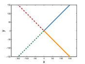
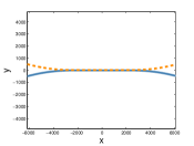
Figure 5: Simulated true target tracks. In scenario 1 (left) all tracks start in the origin. In scenario 2 (right) the tracks start on the left.

Scenario 3 is used to test the so-called ‘spooky’ effect [19]. The scenario has two targets that are spatially separated by at least 1km for all 50 time steps. The probability of detection was set to $p_{D}=0.9$ and clutter Poisson rate was 10. The measurements were generated such that one target is always detected, and the other target is detected on all time steps, except for steps 20, 40 and 41.

For the first two scenarios, 1000 Monte Carlo runs were carried out in order to compare the performance of the four different GGIW filters: GLMB, LMB, LMB with adaptive birth process (LMB-ab), and CPHD. The GGIW-PHD filter is omitted from the comparison because previous work has shown that both the CPHD and GLMB filter outperform the PHD filter [14]. Figure 6 shows the mean OSPA distances, and the mean cardinality errors for scenario 1. The GLMB and LMB filters have approximately equal performance. The LMB-ab filter has slower convergence due to the unknown birth density, however the filter eventually reaches the same error as the GLMB and LMB with known birth density. This is expected since the other three filters have the advantage of knowing the region where new targets will appear. The CPHD filter can match the GLMB and LMB in terms of the cardinality error, however the mean OSPA is larger.

The execution times for our Matlab implementation of the algorithms (mean ± one standard deviation) for Scenario 1 are 3.95 ± 3.41s for the GLMB filter, 0.19 ± 0.29s for the LMB filter, and 2.20 ± 0.47s for the CPHD filter. Since the LMB-ab filter only uses clusters with more than four measurements as birth candidates, it is even faster than the LMB filter. Since the LMB filter partitions the tracks and measurements into approximately statistically independent groups [23, 31], its computation times are less than those of the CPHD filter.

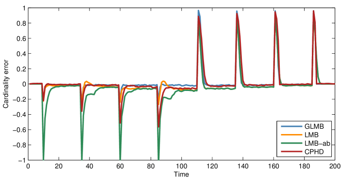
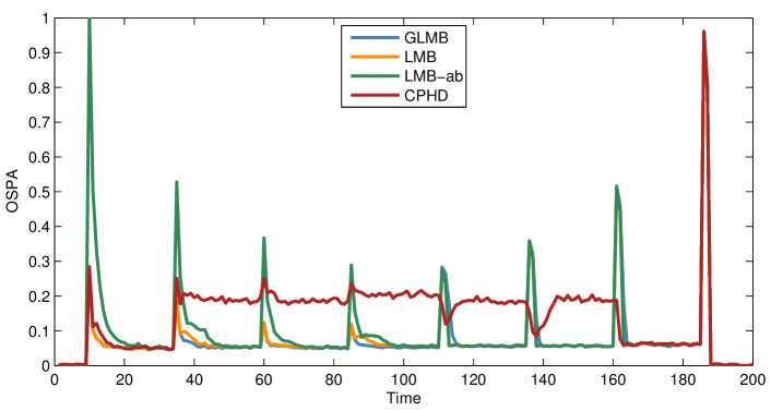
Figure 6: Cardinality error and OSPA metric for scenario 1 (mean values of the 1000 Monte Carlo runs)

Figure 7 shows the mean OSPA distances and mean cardinality errors for scenario 2. Similar to scenario 1, the GLMB filter slightly outperforms the LMB and CPHD filter. Again, the cardinality estimate of the LMB-ab filter takes longer to converge to the correct value, however, the LMB-ab filter has lower OSPA distance and smaller cardinality error than the LMB filter after time 78. This is due to the fact that, in some of the runs, the LMB filter lost one of the tracks because the measurement clusters were very close together. Even after the targets move apart, the filter with static birth density is unable to start a new track on the lost target. However, the filter with adaptive birth density has the capability to start a new track at the lost target’s current location, leading to improved performance.

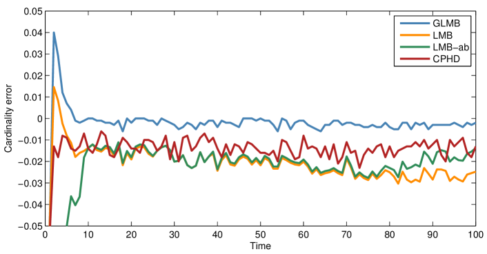
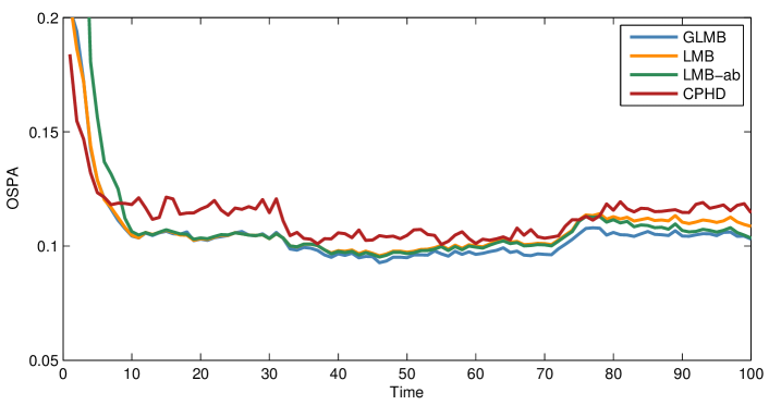
Figure 7: Cardinality error and OSPA metric for scenario 2 (mean values of the 1000 Monte Carlo runs)

In scenario 3 we compare the PHD, CPHD and LMB filters. The estimated weights (for the PHD and CPHD) and existence probabilities (for the LMB) for a single run are shown in Figure 8. The PHD filter suffers from a positive bias (weight around 1.1), and the weight drops quickly when there are missed detections. The CPHD clearly suffers from the ‘spooky’ effect [19], as the weight of the detected target increases when the other target is misdetected. In comparison, the LMB filter performs better, as the probability of existence of the detected target is unaffected when the other target is not detected. Also, the decrease in the existence probability following the missed detections is more conservative compared to the decrease in the weights for the PHD and CPHD filters.

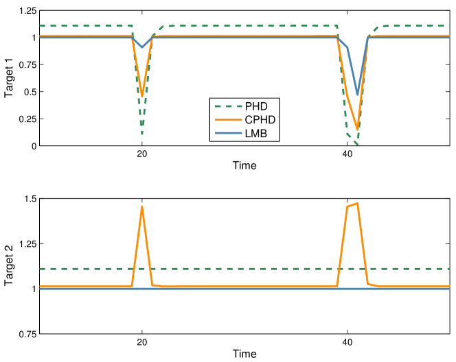
Figure 8: Result from spooky effect scenario. The lines show the estimated weights for two spatially separated targets. The distance between the two targets is 1km, at time steps 20, 40 and 41 there are missed detections for target 1.

VI Experimental Results

Figure 9: Ground truth (dashed) and estimated (solid) pedestrian trajectories. Estimated two-sigma ellipses and corresponding laser measurements (black) are plotted for selected time steps.

To demonstrate the proposed method on a real world scenario, we applied the GGIW-LMB filter to pedestrian tracking with laser rangefinders. In contrast to targets with distinct shapes, such as vehicles or buildings, pedestrians do not exhibit specific structure in laser scans, appearing instead as a random cluster of points. Hence, the GGIW measurement model is well suited to this application, since it assumes that the measurements are distributed normally around the target centroid. For this experiment, two pedestrians were recorded while walking on a parking lot using three Ibeo Lux laser sensors, which are mounted in the front bumper of the vehicle. Before being passed to the tracking filter, the laser returns from each sensor were thinned by removing measurements that lie outside the region of interest, thus excluding measurements from parked vehicles. The sensor was stationary during the experiment, and both pedestrians were wandering around the surveillance region, and are in close proximity to each other mid-way through the scenario. Figure 10 shows camera footage from this instant.

Figure 10: Pedestrian tracking scenario: The two pedestrians are getting close at around t = 6.5 seconds.

A constant velocity dynamic model is used to track the pedestrians, i.e., the parameters of (63) are $d=2$ and

$$F_{k+1|k}=\left[\begin{array}[]{cc}1&T\\ 0&1\end{array}\right],\quad Q_{k+1|k}=\sigma^{2}\left[\begin{array}[]{cc}\frac{T^{4}}{4}&\frac{T^{3}}{2}\\ \frac{T^{3}}{2}&T^{2}\end{array}\right]\otimes\chi_{k+1},$$

where the sampling period is $T=0.08\,s$ and the standard deviation of the process noise is $\sigma=4\,m/s^{2}$. Due to the decreased dimension of the motion model, the measurement matrix in (64) is $H_{k}=\left[\begin{array}[]{cc}1&0\end{array}\right]$, and since the birth locations are unknown, the LMB filter with adaptive birth model is used in this scenario. Other filter parameters are similar to those used in Section (V).

The results from the GGIW-LMB-ab filter are depicted in Figure 9. The dashed lines show approximate ground truth trajectories, which were obtained by manually labelling the pedestrians in the raw laser scans, and the solid lines show the estimated trajectories. In addition, two-sigma ellipses representing the target extents as well as the corresponding measurements are also shown for selected time instants.

The filter is able to track both pedestrians continuously, even when they are very close. Especially in this situation, the multi-target representation as (G)LMB facilitates finding consistent association hypotheses and maintaining tracks over time. Note that the strongly fluctuating measurements on different moving parts of the human body, such as legs, arms and torso, make precise estimation of the target centroid positions difficult, in both the manual labelling process, and for the tracker itself. This explains most of the deviation between labelled ground truth and estimated trajectories. The estimates of the pedestrian extent vary over time, as demonstrated by the changing ellipses in Figure 9. This is again due to fluctuating measurements, which can be attributed mostly to leg movement. When the targets are close to the sensors, and the laser rangefinders provide detailed scans of the legs, a periodic adaption of the target extent following the motion of the legs with each stride could be observed.

VII Conclusion

In this paper we have proposed two algorithms for tracking multiple extended targets in clutter, namely the GGIW-GLMB and GGIW-LMB filter. Both are based on modelling the problem using labelled random finite sets, and gamma Gaussian inverse Wishart mixtures. The proposed algorithms estimate the number of targets, and their kinematics, extensions and measurement rates. The major advantage of these methods over the previously developed GGIW-(C)PHD filters is the inclusion of target labels, allowing for continuous target tracks, which is not directly supported by the (C)PHD filters.

Of the two proposed algorithms, the GGIW-GLMB filter is more accurate as it involves fewer approximations, but it is also more computationally demanding than the GGIW-LMB filter. Simulation results demonstrate that the algorithms outperform the GGIW-(C)PHD filters, especially in cases where the performance of the CPHD filter is degraded due to the spooky effect. Finally, we have also demonstrated that the filter performs well in a real-world application, in which laser rangefinders are used to track pedestrians.

References

- [1] M. Beard, B.-T. Vo, B.-N. Vo, “Bayesian multi-target tracking with merged measurements using labelled random finite sets,” IEEE Trans. Signal Process., vol. 63, no. 6, pp. 1433-1447, March 2015.
- [2] K. Gilholm and D. Salmond, “Spatial distribution model for tracking extended objects,” IEE Proc. Radar, Sonar and Navigation, vol. 152, no. 5, pp. 364–371, Oct. 2005.
- [3] K. Gilholm, S. Godsill, S. Maskell, and D. Salmond, “Poisson models for extended target and group tracking,” Proc. Signal and Data Processing of Small Targets, vol. 5913, pp. 230–241, San Diego, CA, Aug. 2005.
- [4] J. W. Koch, “Bayesian approach to extended object and cluster tracking using random matrices,” IEEE Trans. Aerosp. Electron. Syst., vol. 44, no. 3, pp. 1042–1059, July 2008.
- [5] W. Wieneke, J. W. Koch, “Probabilistic tracking of multiple extended targets using random matrices,” SPIE Signal and Data Processing of Small Targets, Orlando, FL, USA, Apr. 2010.
- [6] M. Feldmann, D. Fr nken, and J. W. Koch, “Tracking of extended objects and group targets using random matrices,” IEEE Trans. Signal Process., vol. 59, no. 4, pp. 1409–1420, Apr. 2011.
- [7] J. W. Koch, M. Feldmann, “Cluster tracking under kinematical constraints using random matrices,” Robotics and Autonom. Syst., vol. 57, no. 3, pp. 296–309, Mar. 2009.
- [8] M. Baum, B. Noack, and U. D. Hanebeck, “Extended object and group tracking with elliptic random hypersurface models,” 13th Int. Conf. Inform. Fusion, Edinburgh, UK, July 2010.
- [9] M. Baum and U. D. Hanebeck, “Shape tracking of extended objects and group targets with star-convex RHMs,” Proc. 14th Int. Conf. on Inform. Fusion, Chicago, IL, USA, July 2011.
- [10] C. Lundquist, K. Granstr m, U. Orguner, “Estimating the shape of targets with a PHD filter,” 14th Int. Conf. Inform. Fusion, Chicago, IL, USA, July 2011.
- [11] R. Mahler, “Multitarget Bayes filtering via first-order multitarget moments”, IEEE Trans. Aerosp. Elecron. Syst. vol. 39, no. 4, pp. 1152-1178, Oct. 2003.
- [12] R. Mahler, “PHD filters for nonstandard targets, I: Extended targets,” 12th Int. Conf. Inform. Fusion, Seattle, WA, USA, July 2009.
- [13] K. Granstr m, U. Orguner, “A PHD filter for tracking multiple extended targets using random matrices,” IEEE Trans. Signal Process., vol. 60, no. 11, pp. 5657–5671, Nov. 2012.
- [14] C. Lundquist, K. Granstr m, U. Orguner, “An extended target CPHD filter and a gamma Gaussian inverse Wishart implementation,” IEEE J. Sel. Topics Signal Process., vol. 7, no. 3, pp. 472-483, Feb. 2013.
- [15] K. Granstr m, U. Orguner, “Estimation and maintenance of measurement rates for multiple extended target tracking,” 15th Int. Conf. Inform. Fusion, Singapore, July 2012.
- [16] K. Granstr m, C. Lundquist, U. Orguner, “Extended Target Tracking using a Gaussian-Mixture PHD Filter ”, IEEE Trans. Aerosp. Elecron. Syst., vol. 48, no. 4, pp. 3268 - 3286, Oct. 2012.
- [17] K. Granstr m and U. Orguner, “On the reduction of Gaussian inverse Wishart mixtures,” 15th Int. Conf. Inform. Fusion, Singapore, July 2012.
- [18] B.-T. Vo, B.-N. Vo, A. Cantoni, “Analytic implementations of the cardinalized probability hypothesis density filter,” IEEE Trans. Signal Process., vol. 55, no. 7, pp. 3553-3567, July 2007.
- [19] B.-T. Vo, B.-N. Vo, “The para-normal Bayes multi-target filter and the spooky effect,” 15th Int. Conf. Inform. Fusion, Singapore, July 2012.
- [20] B. Ristic, J. Sherrah, “Bernoulli filter for joint detection and tracking of an extended object in clutter,” IET Radar, Sonar and Navigation, vol. 7, no. 1, pp. 26-35, Jan. 2013.
- [21] B.-T. Vo and B.-N. Vo, “Labeled random finite sets and multi-object conjugate priors,” IEEE Trans. Signal Process., vol. 61, no. 13, pp. 3460-3475, July 2013.
- [22] B.-N. Vo; B.-T. Vo, D. Phung, “Labeled random finite sets and the Bayes multi-target tracking filter,” IEEE Trans. Signal Process., vol. 62, no. 24, pp. 6554-6567, Dec. 2014.
- [23] S. Reuter, B.-T. Vo, B.-N. Vo, K. Dietmayer, “The labeled multi-Bernoulli filter,” IEEE Trans. Signal Process., vol.62, no.12, pp. 3246,3260, June 2014.
- [24] M. Beard, S. Reuter, K. Granstr m, B.-T. Vo, B.-N. Vo, A. Scheel, “A generalised labelled multi-Bernoulli filter for extended multi-target tracking”, to appear 18th Int. Conf. Inform. Fusion, Washington DC, USA, July 2015.
- [25] R. P. S. Mahler, Statistical Multisource-Multitarget Information Fusion, Artech House, 2007.
- [26] B.-N. Vo, S. Singh, and A. Doucet, “Sequential Monte Carlo methods for Bayesian multi-target filtering with random finite sets”, IEEE Trans. Aerosp. Electron. Syst., vol. 41, no. 4, pp. 1224-1245, Oct. 2005.
- [27] R. Mahler, “PHD filters of higher order in target number”, IEEE Trans. Aerosp. Electron. Syst., vol. 43, no. 4, pp.1523-1543, Oct. 2007.
- [28] B.-T. Vo, B.-N. Vo, A. Cantoni. “The cardinality balanced multi-target multi-Bernoulli filter and its implementations”, IEEE Trans. Signal Process., vol. 57, no. 2, pp. 409-423, Feb. 2009.
- [29] K. G. Murty, “An algorithm for ranking all the assignments in increasing order of cost,” Operations Research, vol. 16, no. 3, pp. 682-678, 1968.
- [30] D. Schuhmacher, B.-T. Vo, B.-N. Vo, “A consistent metric for performance evaluation of multi-object filters,” IEEE Trans. Signal Process., vol. 56, no. 8, pp. 3447-3457, Aug. 2008.
- [31] A. Scheel, K. Granstr m, D. Meissner, S. Reuter, K. Dietmayer, “Tracking and data segmentation using a GGIW filter with mixture clustering,” 17th Int. Conf. Inform. Fusion, Salamanca, Spain, July 2014.
- [32] A. Swain and D. Clark, “Extended object filtering using spatial independent cluster processes,“ Proc. 13th Int. Conf. Inform. Fusion, Edinburgh, UK, July 2010.
- [33] A. Swain and D. Clark, “The PHD filter for extended target tracking with estimable shape parameters of varying size,” 15th Int. Conf. Inform. Fusion, Singapore, July 2012.
- [34] A. Gupta and D. Nagar, Matrix Variate Distributions, Chapman & Hall, 2000.