Detecting concentration changes with cooperative receptors

Abstract

Cells constantly need to monitor the state of the environment to detect changes and timely respond. The detection of concentration changes of a ligand by a set of receptors can be cast as a problem of hypothesis testing, and the cell viewed as a Neyman-Pearson detector. Within this framework, we investigate the role of receptor cooperativity in improving the cell’s ability to detect changes. We find that cooperativity decreases the probability of missing an occurred change. This becomes especially beneficial when difficult detections have to be made. Concerning the influence of cooperativity on how fast a desired detection power is achieved, we find in general that there is an optimal value at finite levels of cooperation, even though easy discrimination tasks can be performed more rapidly by noncooperative receptors.

1 Introduction

The ability to acquire, process and stock information is crucial for living beings. Already at the level of a single cell the external environment is chemically sensed and the acquired information is processed to prepare a suitable response. All the steps involved in these processes are permeated with noise: the arrival of the external stimulus through diffusion is a stochastic process and so is the interaction with the receptors. The successive biochemical steps for the signal transduction usually involve a limited amount of proteins so that fluctuations play a prominent role. In other words, cells need to extract useful information from noisy inputs through noisy mechanisms, a seemingly daunting task. Despite these hurdles, cells are able to sense the environment and make decisions with remarkable precision. For a proper investigation of sensing it is fundamental to precisely characterize it and to assess its performance. The first step towards a quantitative understanding of this issue was taken by Berg and Purcell in their seminal paper in 1977 berg_purcell addressing the question of how precise can a cell be in determining the concentration of an external ligand. Several studies have followed their line of reasoning and considered signal to noise ratios as a measure of the quality of sensing (see e.g. aquino11 ; aquino14 ; bialek05 ; bialek08 ; endres09 ; govern12 ; hu10 ; kaizu14 ; mora10 ; mugler13 ; rappel08 ; sevier14 ; skoge11 ; skoge13 ; sun14 ; tanase06 ). A complementary approach within the framework of information theory has been taken, investigating the ability of signaling networks to acquire information about the environment and transmit it downstream (see Ref. bialek for a general discussion, bowsher14 ; levchenko14 for recent reviews and bowsher12 ; cheong11 ; dubuis13 ; mancini13 ; martins11 ; mugler13 ; rieckh14 ; selimkhanov14 ; tkacik08 ; tkacik11 ; tkacik12 ; tostevin09 ; uda13 ; voliotis14 ; walczak10 ; ziv07 for a representative though necessarily incomplete list of recent contributions). Furthermore, the influence of receptor cooperativity has been studied (see e.g.  aquino11 ; bialek08 ; sevier14 ; skoge11 ; skoge13 ; sun14 ). Quantifying the ability to sense, transmit signals and respond to the external environment enables a quantitative comparison with its costs barato13pre ; barato14 ; barato15 ; govern14pnas ; govern14prl ; hartich15 ; lan12 ; lang14 ; mancini15 ; mehta ; murugan12 ; ouldridge15 ; qian05 ; qian06 ; sartori_pigolotti ; sartori14 ; skoge13 ; tu08 . This contributes to the understanding of the trade-offs which, under evolutionary pressure, may have shaped the signaling and transcriptional strategies which are presently observed.

Here we focus on a different task: rather than precisely inferring the value of an external concentration, cells have to efficiently detect changes from a reference level. Such systems include for instance the ones involved in enforcing homeostasis which must monitor deviations from the physiological conditions, the early stages of the immune response with the detection of an antigen and more generally signaling pathways downstream of receptors that undergo adaptation to the external stimuli. The problem of detecting a change can be cast in terms of hypothesis testing. Namely, one tests the hypothesis that a change has occurred vs the null one. This problem has been thoroughly studied in Ref. siggia13 , where it has been shown how the occupation history of a single receptor can be used to perform a sequential probability ratio test. In such dynamic formulation they derived how quickly a decision between two hypotheses can be made given an error threshold. To carry out a statistical test exploiting the history of a receptor, cells need to devise molecular strategies to record it and analyze it. Refs. kobayashi10 ; siggia13 suggested some possible mechanisms to encode statistical analysis in the level of some readout molecules which can be used to make decisions. At variance with this approach, which focuses on sequential testing and considers a single receptor, here we study the case of parallel testing through the instantaneous occupation state of a large pool of independent receptors. This static approach no longer requires the presence of additional molecular layers as the receptors state at a given time can be used directly as a readout. As a shortcoming, restricting to the instantaneous receptors occupation provides a less powerful test than the one exploiting the full receptor history.

We then view the cell as a Neyman-Pearson detector which compares the likelihood of the observed receptor occupancy distribution under the two hypotheses: the environment has not changed vs a change occurred. Within this framework we quantify the detection performance in terms of the probability of missing the detection of a change.

The specific question that we address is whether cooperativity between the binding sites of a given receptor can be beneficial for effectively detecting changes. We find that cooperativity indeed increases the detection sensitivity making it the preferable mechanism when difficult detections have to be performed. When considering the time needed to achieve a certain statistical power we unveil a trade-off which results in an optimal finite level of cooperativity which depends on the required sensitivity and on the number of binding sites present in each receptor. In summary, we find that easy detections are often achieved more rapidly by receptors with low levels of cooperativity (or even noncooperative binding sites) whereas for difficult discrimination tasks a high cooperativity is mandatory.

2 Neyman-Pearson hypothesis testing for concentration discrimination

To illustrate the main ideas of our approach let us start with a simple example. Consider the case in which a cell has to determine whether the concentration of a given ligand has changed or not by means of the occupation state of its receptors. Such problem can be addressed in terms of testing the null hypothesis that no change occurred vs the alternative one that the concentration has changed. For the sake of simplicity let us restrict to the specific case in which the concentration has been constant for a long time and the change is an instantaneous switch from a value $c$ to $c^{\prime}$ taking place at time $t=0$.

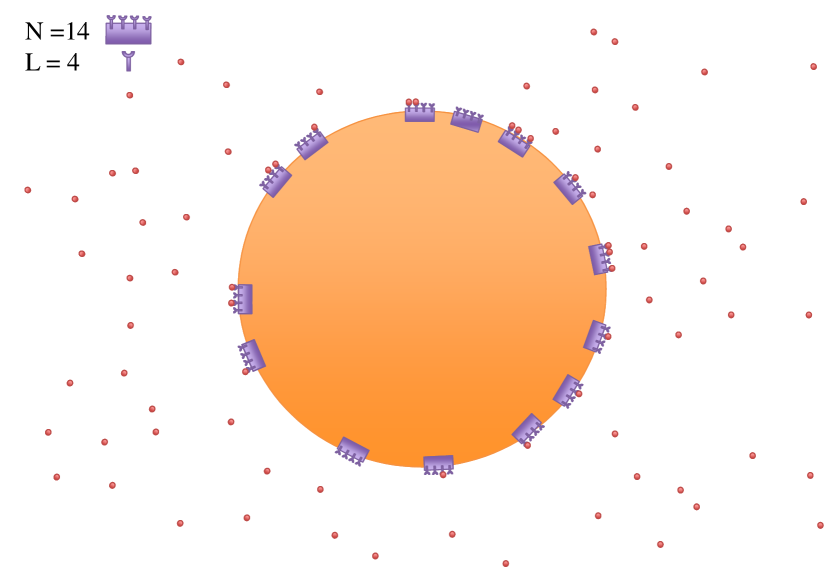
Figure 1: Schematic view of a cell and its sensing components. The cartoon depicts a case with $N=14$ independent receptors each equipped with $L=4$ binding sites.

If a cell is equipped with $N\gg 1$ independent receptors each with $L$ different binding sites (see figure 1), the state of the system at a given time is specified by ${\cal L}=l_{1},l_{2},\ldots l_{N}$ where each $l_{n}=0,1,\ldots L$ denotes the number of occupied binding sites in receptor $n$. Since the receptors are independent we have that $\cal{L}$ is a collection of $N$ independent identically distributed variables drawn from the probability of the occupation number of a single receptor $p_{t}(l)$. Inferring if the concentration of the external ligand has changed corresponds to choosing between two hypothesis

$$H_{0}:\,p_{t}(l)=p_{0}=p_{eq}^{c}(l)$$ (1)

$$H_{1}:\,p_{t}(l)=p_{1}=p_{t}^{c^{\prime}}(l)$$

where $p_{eq}^{c}(l)$ is the equilibrium probability of a receptor having $l$ occupied binding sites when the concentration is $c$ and $p_{t}^{c^{\prime}}(l)$ is the time dependent one for a system that started in equilibrium with $c$ but for which the concentration switched to $c^{\prime}$ at $t=0$. Neyman-Pearson lemma ensures that for a given significance $\alpha$ (probability of mistakenly rejecting the null hypothesis when it is true, type I error) the most powerful test (i. e. minimizing the probability $\beta$ of discarding the alternative hypothesis when it is the correct one, type II error) is the likelihood ratio cover . Such test implies that for a single receptor the null hypothesis is rejected when $l$ is such that

$$\Lambda(l)=\frac{p_{eq}^{c}(l)}{p_{t}^{c^{\prime}}(l)}\leq\eta$$ (2)

where $\eta$ determines the significance

$$\alpha=Prob(\Lambda\leq\eta|H_{0})=\sum_{l}p_{eq}^{c}(l)\Theta\left(\eta p_{t}^{c^{\prime}}(l)-p_{eq}^{c}(l)\right)$$ (3)

where $\Theta$ is the Heaviside step function (i.e. $\Theta(x)=1$ if $x\geq 0$ and $\Theta(x)=0$ if $x<0$). According to Stein’s lemma, when the number of independent receptors is large ($N\gg 1$) the probability of not detecting the change when it has occurred decreases exponentially as $\beta\sim e^{-ND_{KL}(p_{0}||p_{1})}$ where the Kullback-Leibler divergence is defined as

$$D_{KL}(p_{0}||p_{1})=\sum_{l}p_{0}(l)\log\frac{p_{0}(l)}{p_{1}(l)}$$ (4)

which for this specific example reads:

$$D_{KL}(p_{eq}^{c}||p_{t}^{c^{\prime}})=\sum_{l}p_{eq}^{c}(l)\log\frac{p_{eq}^{c}(l)}{p_{t}^{c^{\prime}}(l)}\;.$$ (5)

The divergence, and consequently the test sensitivity, changes with time (see fig. 2). At the very beginning the two distributions are equal and discrimination is therefore impossible. For short times the likelihoods of the two hypotheses are still very similar and the Kullback-Leibler divergence grows quadratically in time (due to probability conservation there is no linear contribution). For long times the probability of the alternate hypothesis approaches the equilibrium value $\lim_{t\to\infty}p_{t}^{c^{\prime}}=p_{eq}^{c^{\prime}}$ and the divergence saturates at the value $D_{KL}(p_{eq}^{c}||p_{eq}^{c^{\prime}})$. The existence of a stationary distribution $p_{eq}^{c^{\prime}}$ ensures that the Kullback-Leibler divergence grows monotonically in time. This means that the asymptotic value $D_{KL}(p_{eq}^{c}||p_{eq}^{c^{\prime}})$ sets the maximum detection precision attainable for the given concentration change. For intermediate times, the divergence changes concavity (at least once) from positive to negative.

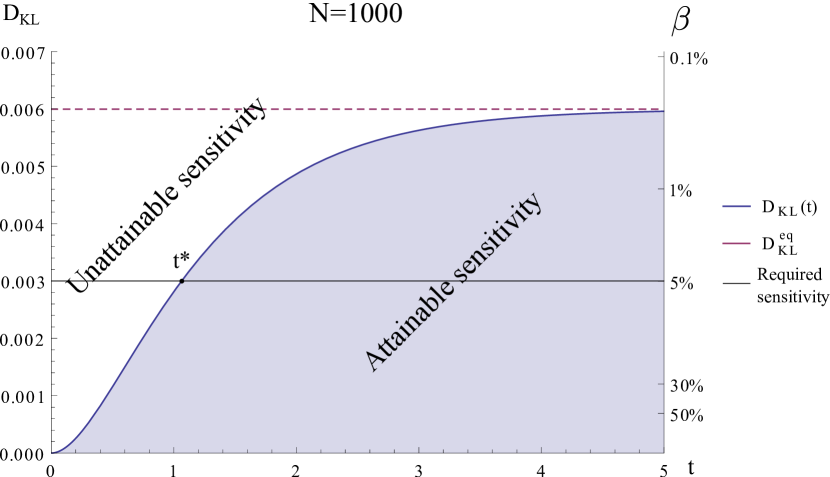
Figure 2: Time evolution of the Kullback Leibler divergence $D_{KL}(p_{eq}^{c_{1/2}}||p_{t}^{c^{\prime}})$ and of the associated miss probability $\beta$ for $N=1000$ receptors. The level of the divergence sets the detection sensitivity. The shaded blue area refers to levels of sensitivity which can be reached by the system. As discussed in the text, the concentration change cannot be immediately detected as the initial divergence is zero. As time goes by, the discrimination power increases until an equilibrium value is reached. If one is interested in a specific sensitivity (thin black line in the plot set at a miss probability of $5\%$ corresponding to $D_{KL}=0.003$) there is an associated time needed to cross the threshold $t^{*}$. The plot is a numerical solution for the Pauling model described in section 3 for a receptor with $L=3$ binding sites cooperating with a coupling of $J=1$. The concentration change to detect is $c^{\prime}=0.9*c_{1/2}$. Time is expressed in units of $\left(k_{u}\sqrt{c^{\prime}/c_{1/2}}\right)^{-1}$ i.e. about the time needed for a (un-)binding event in the noncooperative case.

3 Pauling model of cooperative receptors

Let us now take a closer look at the probability distribution of the occupation level of an individual receptor and study its dependence on the external concentration. We consider each receptor to consist of $L$ binding sites and its read-out to be given by its number of occupied binding sites $l=0,\,1\,\ldots L$. To investigate the role of cooperativity we choose the Pauling model in which each binding site of the receptor interacts with all the other ones phillips_book . A given binding site $i=1,\ldots L$, can be occupied ($\sigma_{i}=0,\;1$) with a probability that depends on the external concentration of the ligand, on its binding energy and, through cooperativity, on the number of other sites of the receptor which are bound. The system can be described in terms of an Ising model with Hamiltonian:

$$H=-h\sum_{i=1}^{L}\sigma_{i}-\frac{J}{2}\sum_{i\neq j}\sigma_{i}\sigma_{j}$$ (6)

where, for the sake of simplicity, we have encoded in $h$ both the contribution of the binding energy and the one of the chemical potential which is affected by the ligand concentration:

$$h=\log\frac{c}{K_{d}}$$ (7)

where $K_{d}$ is the dissociation constant for the noncooperative receptor and we have set $k_{B}T$ to unity for the rest of the paper. We refer to phillips_book for a detailed connection between the statistical mechanical and the chemical description of the systems. Notice that, in this system, cooperativity is encoded in the fact that the probability of binding increases with the number of bound sites. Such cooperativity grows with the number of interacting binding sites and with the coupling parameter $J$. Setting $J=0$ corresponds to considering the noncooperative case of independent binding sites. The energy of a configuration depends only on the occupation number $l=\sum_{i=1}^{L}\sigma_{i}$ giving

$$H(l)=-hl-\frac{J}{2}l(l-1)$$ (8)

and the number of configurations with the same occupation number is simply given by the binomial coefficient ${L\choose l}$. The equilibrium occupation probability then reads

$$p_{eq}(l)=\frac{{L\choose l}\exp\left[hl+\frac{J}{2}l(l-1)\right]}{\sum_{l=0}^{L}{L\choose l}\exp\left[hl+\frac{J}{2}l(l-1)\right]}$$ (9)

and the average number of bound sites can be directly computed as

$$\langle l\rangle=\sum_{l=0}^{L}lp_{eq}(l)\;.$$ (10)

The cooperativity of the system allows to have sharp changes in the occupation probability as the external concentration is varied. The system is then said to be ultrasensitive around the value of the external field for which half of the binding sites are bound on average $h_{1/2}$, which we refer to as the transition point. Such value depends on the number of total binding sites $L$ and the coupling $J$

$$h_{1/2}=-\frac{J}{2}(L-1)$$ (11)

and ensures that $p_{eq}(l)=p_{eq}(L-l)$. We note that for highly cooperative systems the equilibrium distribution at $h=h_{1/2}$ is concentrated at the extremes $l=0$ and $l=L$. The transition point occurs at different values of concentration as the number of binding sites or the coupling are changed

$$c_{1/2}(J,L)=K_{d}e^{-\frac{J}{2}(L-1)}\;.$$ (12)

To proceed to a meaningful comparison between different cooperativities we need to consider systems that have to detect changes of the same relative amplitude $c/c_{1/2}$. In general, cooperative receptors with different numbers of binding sites or cooperative strengths can set their transition point at the same concentration by tuning their dissociation constant. This is a simple mechanism that implements sensorial adaptation. Indeed, by letting $K_{d}(L,J)=K_{d}^{(0)}e^{\frac{J}{2}(L-1)}$ the transition point is reached for the same concentration $c_{1/2}=K_{d}^{(0)}$. This means that in order to maintain ultra-sensitivity around a given concentration the receptor has to compensate for a higher cooperativity by evolving towards a higher dissociation constant (lower affinity with ligand).

3.1 Cooperativity and discrimination

As discussed above, around the transition point, the distribution of the occupation number of the receptor exhibits a stronger dependence on concentration as cooperativity is increased. Such sharper dependence makes it easier to tell if the concentration has changed from the reference value (set at the transition point). Intuitively, then, cooperativity improves the discrimination ability of the receptor. To check this intuition let us consider the behavior of the Kullback-Leibler distance between the equilibrium probability at the transition point and the one of a different concentration and its dependence on the degree of cooperativity (see figure 3). We start by considering the asymptotic value of the divergence which corresponds to the largest possible discrimination. Due to Stein’s lemma, the Kullback-Leibler divergence describes how the probability of missing a change in concentration decreases with the number of independent measurements $N$ in the limit $N\to\infty$. For instance to achieve a miss probability $\beta\simeq 5\%$ we need a divergence between the two distributions of

$$D_{KL}(p^{c_{1/2}}_{eq}||p^{c^{\prime}}_{eq})=-\frac{\log\beta}{N}\simeq\frac{3}{N}\;.$$ (13)

For a given number of independent receptors $N$ the Kullback-Leibler divergence then sets the miss probability.

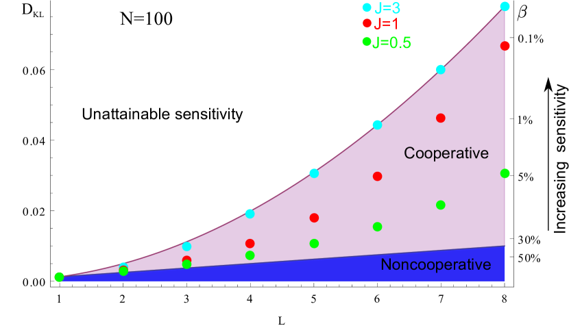
Figure 3: Long-time asymptotic Kullback Leibler divergence and miss probability for $N=100$ receptors as a function of binding sites numbers for $c^{\prime}=0.9*c_{1/2}$. The full purple line is the divergence in the limit of infinite coupling ($J\to\infty$) discussed in eq. (3.1) and the full blue one is the noncooperative case ($J=0$) discussed in eq. (15). The shaded blue area depicts the values of precision reachable with noncooperative binding sites, the purple shaded one the values achievable by cooperative receptors. The white area above the purple line refers to precisions which cannot be reached for the given number of binding sites. The cyan points are numerically evaluated results for $J=3$ already approaching the infinite coupling limit. The red points refer to the case with $J=1$ and the green ones to $J=0.5$.

Let us start by considering the noncooperative case ($J=0$). The system then simplifies greatly and is just a collection of $L$ independent two states processes with binomial distribution

$$p_{eq}^{\mathit{nc}}(l)={L\choose l}\frac{\left(\frac{c}{c_{1/2}}\right)^{l}}{\left(\frac{c}{c_{1/2}}+1\right)^{L}}\;.$$ (14)

The Kullback-Leibler divergence is then analytically accessible and considering the two equilibrium distributions reads:

$$D_{KL}^{\mathit{nc}}(p^{c_{1/2}}_{eq}||p^{c^{\prime}}_{eq})=L\log\left(\frac{\sqrt{\frac{c_{1/2}}{c^{\prime}}}+\sqrt{\frac{c^{\prime}}{c_{1/2}}}}{2}\right)=L\log\left[\cosh\left(\frac{h^{\prime}-h_{1/2}}{2}\right)\right]$$ (15)

where we shall recall that $h_{1/2}=0$. The most relevant feature is that the divergence grows linearly with the number of binding sites present in the receptor.

We expect cooperativity to increase the Kullback-Leibler divergence and consequently decrease the probability of not detecting a concentration change. In the limit of large coupling $J\to\infty$ we can roughly estimate the occupation probability by inspecting equation (9) around $h_{1/2}=-J(L-1)/2$ and observing that only states with $l=0$ and $l=L$ will have a finite probability:

$$\lim_{J\to\infty}p(l=0)\simeq\frac{1}{1+e^{L(h^{\prime}-h_{1/2})}}=\frac{1}{1+\left(\frac{c^{\prime}}{c_{1/2}}\right)^{L}}$$ (16)

$$\lim_{J\to\infty}p(l=L)\simeq\frac{e^{L(h^{\prime}-h_{1/2})}}{1+e^{L(h^{\prime}-h_{1/2})}}=\frac{\left(\frac{c^{\prime}}{c_{1/2}}\right)^{L}}{1+\left(\frac{c^{\prime}}{c_{1/2}}\right)^{L}}$$

giving

$$\lim_{J\to\infty}D_{KL}(p^{c_{1/2}}_{eq}||p^{c^{\prime}}_{eq}) = \log\left(\frac{\left(\frac{c_{1/2}}{c^{\prime}}\right)^{L/2}+\left(\frac{c^{\prime}}{c_{1/2}}\right)^{L/2}}{2}\right)$$

$$= \log\left[\cosh\left(\frac{L(h^{\prime}-h_{1/2})}{2}\right)\right]$$

which for $L>1$ is larger than its noncooperative equivalent. Hence, for a fixed $L$, having a cooperative receptor allows to reach values of the Kullback-Leibler that cannot be approached by means of noncooperative binding sites resulting in higher detection sensitivities. However, the limit in eq. (3.1) cannot be exceeded and this sets an upper bound on the performance of a cooperative receptor following Pauling model.

3.1.1 Small concentration change limit

The hypotheses we are testing have probability distributions that differ because of the parameter $c$ and $c^{\prime}$. Obviously, when the two concentrations are equal the Kullback-Leibler divergence is zero and is at a minimum since it is non-negative by definition. Then, for small concentration differences $\delta c/c\ll 1$, the divergence is quadratic in the concentration difference. It is known that curvature of the divergence in $c=c^{\prime}$ is equal to the Fisher information of the probability distribution with respect to the parameter $c$ which is defined as

$${\cal I}(c)=\sum_{l=0}^{L}\left(\frac{\partial\log{p^{c}_{eq}(l)}}{\partial c}\right)^{2}p^{c}_{eq}(l)\,.$$ (18)

Then, by Taylor expansion, the Kullback-Leibler for small concentration changes around $c$ reads

$$\lim_{\delta c/c\to 0}D_{KL}(p^{c}_{eq}||p^{c+\delta c}_{eq})\simeq\frac{1}{2}\left(\delta c\right)^{2}{\cal I}(c)\;.$$ (19)

Plugging relation (7) into the equilibrium probability (9) we can compute the derivative of the probability with respect to concentration and obtain:

$$\frac{\partial p^{c}_{eq}(l)}{\partial c}=\frac{l-\langle l\rangle}{c}p^{c}_{eq}(l)$$ (20)

which means that the Fisher information is ${\cal I}(c)=\frac{1}{c^{2}}var(l)$ and the Kullback-Leibler for small concentration changes around the transition point $c_{1/2}$

$$\lim_{\delta c/c\to 0}D_{KL}(p^{c_{1/2}}_{eq}||p^{c_{1/2}+\delta c}_{eq})\simeq\frac{1}{2}\left(\frac{\delta c}{c_{1/2}}\right)^{2}var(l)\;.$$ (21)

It is interesting to compare the two extremes of large cooperativity and vanishing cooperativity. Taking the large coupling limit $J\to\infty$ of the variance we see that

$$\lim_{J\to\infty}\lim_{\delta c/c\to 0}D_{KL}(p^{c_{1/2}}_{eq}||p^{c_{1/2}+\delta c}_{eq})\simeq\lim_{J\to\infty}\frac{1}{2}\left(\frac{\delta c}{c_{1/2}}\right)^{2}var(l)\simeq\frac{1}{8}\left(\frac{\delta c}{c_{1/2}}\right)^{2}L^{2}$$ (22)

where two limits can be shown to commute by considering eq. (3.1). For the noncooperative case one finds

$$\lim_{\delta c/c\to 0}D^{\mathit{n}c}_{KL}(p^{c_{1/2}}_{eq}||p^{c_{1/2}+\delta c}_{eq})\simeq\frac{1}{8}\left(\frac{\delta c}{c_{1/2}}\right)^{2}L\;.$$ (23)

The strongly cooperative case displays a quadratic dependence on the number of binding sites, as opposed to the linear one of the noncooperative model. The miss probability of the test then decreases exponentially with $L^{2}N$ for the cooperative case and simply as $LN$ for the noncooperative one. For finite couplings, the variance has to be computed directly from the distribution and reads:

$$var(l)={\sum_{l=0}^{L}\left(l-\langle l\rangle\right)^{2}p_{eq}(l})$$ (24)

$$=\frac{\sum_{l=0}^{L}l^{2}{L\choose l}\exp\left[hl+\frac{J}{2}l(l-1)\right]}{\sum_{l=0}^{L}{L\choose l}\exp\left[hl+\frac{J}{2}l(l-1)\right]}-\left(\frac{\sum_{l=0}^{L}l{L\choose l}\exp\left[hl+\frac{J}{2}l(l-1)\right]}{\sum_{l=0}^{L}{L\choose l}\exp\left[hl+\frac{J}{2}l(l-1)\right]}\right)^{2}$$

Such expression, due to the terms $\exp\left[\frac{J}{2}l(l-1)\right]$ does not display a simple scaling in terms of $L$ for finite couplings.

3.1.2 Connection between Hill coefficient and Kullback-Leibler divergence

The Hill coefficient is a measure of the cooperativity of binding and can be defined (see e.g. Ref. hill85 ) as:

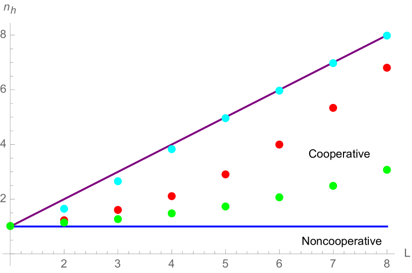
Figure 4: Hill coefficient as a function of binding sites per receptor $L$ for different values of the coupling $J$. For the noncooperative case the Hill coefficient is $1$ whereas it is $L$ in the limit of strong cooperativity. The parameters and color code are the same as for figure 3.

$$n_{H}=\frac{4}{L}\frac{\partial\langle l\rangle}{\partial\log c}\biggr{|}_{c=c_{1/2}}=\frac{4}{L}\frac{\partial\langle l\rangle}{\partial h}\biggr{|}_{c=c_{1/2}}\;.$$ (25)

Performing the derivative of the mean value with the explicit expressions given in eqs. (9) and (10) we see that

$$\frac{\partial\langle l\rangle}{\partial h}=var(l)\;.$$ (26)

We can then write

$$n_{H}=\frac{4}{L}var(l)\;.$$ (27)

As we have seen in eq. (19), for small concentration changes, the Kullback-Leibler divergence is proportional to the Fisher information which, for the system we are considering, is itself proportional to the variance of the distribution ${\cal I}=var(l)/c^{2}$. Hence, for small concentration changes around the transition point, we have that

$$\lim_{\delta c/c\to 0}D_{KL}(p^{c_{1/2}}_{eq}||p^{c_{1/2}+\delta c}_{eq})\simeq\frac{1}{2}\left(\frac{\delta c}{c}\right)^{2}var(l)=\frac{L}{8}\left(\frac{\delta c}{c}\right)^{2}n_{H}$$ (28)

linking the Kullback-Leibler divergence and the Hill coefficient. The Hill coefficient ranges from $1$ for noncooperative binding to a maximum of $L$ approached in the limit of infinite cooperativity (see fig. 4). This offers some insight on the scaling behavior of the Kullback-Leibler divergence for finite couplings. Indeed, for small concentration changes, the Kullback-Leibler divergence scales as $Ln_{H}$ where $n_{H}$ is the Hill coefficient of the receptor.

3.2 How long does it take to detect a change?

From figure 2 we know that at the moment in which the concentration changes it is not possible yet to detect the change as the distributions of the two hypotheses are still equal. Detection becomes possible as the likelihood of the alternative hypothesis evolves in time. We are interested in studying how long it takes before the distributions of the two hypotheses are different enough to allow a detection with a given sensitivity. In order to do so, let us now consider the kinetic behavior of a receptor whose binding sites follow the Pauling model. In general the occupation probability evolves according to a master equation

$$\frac{dp(l)}{dt}=\sum_{l}k(l^{\prime}\to l)p(l^{\prime})-k(l\to l^{\prime})p(l)$$ (29)

where, for the system to reach the correct equilibrium, detailed balance must be satisfied by the rates:

$$\frac{k(l\to l^{\prime})}{k(l^{\prime}\to l)}=\frac{p_{eq}(l^{\prime})}{p_{eq}(l)}=e^{-\left(H(l^{\prime})-H(l)\right)}{L\choose l^{\prime}}/{L\choose l}$$ (30)

which for the two allowed transitions implies

$$\frac{k(l\to l+1)}{k(l+1\to l)}=\frac{L-l}{l+1}e^{h+Jl}=\frac{(L-l)c}{(l+1)c_{1/2}(J,L)}e^{J\left(l-\frac{L-1}{2}\right)}\;.$$ (31)

There is freedom in how to choose the individual rates still satisfying detailed balance. We consider the case in which the rates are exponential in the energy difference associated with the transition and to make contact with the non-cooperative binding we set them to

$$k(l\to l+1) = (L-l)k_{u}\frac{c}{c_{1/2}(J,L)}e^{\frac{J}{2}\left(l-\frac{L-1}{2}\right)}$$ (32)

$$k(l\to l-1) = l\,k_{u}e^{-\frac{J}{2}\left(l-\frac{L+1}{2}\right)}$$ (33)

where $k_{u}$ is the unbinding rate for noncooperative binding sites. We can then proceed to the numerical solution of the master equation and obtain the time evolution of the system. We shall focus on the case in which the system starts in equilibrium with the concentration at the transition point $c_{1/2}$ and the concentration is switched to a different value $c^{\prime}$. The most remarkable feature is that, for fixed $c^{\prime}/c_{1/2}$, as cooperativity is increased (both by having more binding sites or by a higher coupling $J$) the system slows down. The slowing down is more severe for small concentration changes. This phenomenon is related to the critical slowing down (discussed also in Ref. skoge11 ) and is due to the fact that a system with strong interactions is “locked” into a configuration due to cooperativity and reacts more slowly to a change in the external field.

Let us now investigate how this impacts on the time required by the pool of receptors to reach a certain detection sensitivity. We need to consider the dynamic behavior of the Kullback-Leibler divergence during equilibration to the new concentration $c^{\prime}$ and how rapidly it manages to reach the threshold associated with the desired sensitivity as sketched in figure 2. As we have discussed in the previous section and shown in figure 3, the divergence between the equilibrium distribution in $c_{1/2}$ and in $c^{\prime}$ is higher for cooperative receptors consequently allowing to reach levels of sensitivity which are unfeasible for noncooperative binding sites. However, a larger cooperativity slows down the dynamics. When considering how fast a certain level is reached we are then facing a trade-off as shown in figure 5.

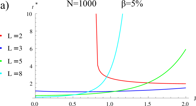
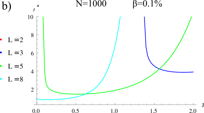
Figure 5: Time needed to achieve a desired sensitivity in detecting a concentration change to $c^{\prime}=0.9*c_{1/2}$ for different numbers of binding sites and cooperativity. This corresponds to time needed by the Kullback Leibler divergence $D_{KL}(p_{eq}^{c_{1/2}}||p_{t}^{c^{\prime}})$ to cross a given threshold. a): miss probability of $5\%$ which for $N=1000$ receptors corresponds to $D_{KL}=0.003$. For $J<0.81$ the receptor with $L=2$ binding sites cannot reach a divergence of $0.003$. For $L=3$ the shortest time is obtained at finite coupling whereas for $L=5\,,8$ for the noncooperative case. Notice the exponential slowing down observed for $L=8$. b): miss probability of $0.1\%$ corresponding for $N=1000$ receptors to $D_{KL}\simeq 0.0069$. Now the required sensitivity is unattainable with $L=2$ binding sites. It requires a coupling $J>1.37$ for $L=3$ and a weak $J>0.1$ for $L=5$. For the shown number of binding sites the desired precision is fastest reached for finite level of cooperativity. Time is expressed in units of $\left(k_{u}\sqrt{c^{\prime}/c_{1/2}}\right)^{-1}$ i.e. about the time needed for a (un-)binding event in the noncooperative case.

To obtain some insight let us study a specific example. Consider for instance the case in which we have $N=1000$ receptors, the concentration decreases of about $10\%$ from its transition value: $c^{\prime}=0.9*c_{1/2}$ and we want to achieve a miss probability of $\beta\simeq 5\%$. This sets the Kullback Leibler distance between the equilibrium receptor distribution at the transition point and the evolving one at $D_{KL}(p_{eq}^{c_{1/2}}||p_{t}^{c^{\prime}})=0.003$. From eq. (15) we know that such sensitivity cannot be achieved by a receptor with $2$ binding sites unless they operate in a cooperative fashion. Then, for small couplings, a receptor with $2$ binding sites will never reach the threshold. As the coupling is increased the threshold becomes attainable and it progressively takes shorter times to approach it until an optimal value is reached. When several binding sites can be employed the situation is quite the opposite as the threshold is largely exceeded also in the noncooperative case so that the main effect of cooperativity is the exponential slowing down of the dynamics. In such case the required sensitivity is reached earlier by noncooperative binding sites. For intermediate scenarios, as for example with $3$ binding sites, the noncooperative case is sufficient to cross the threshold but its asymptotic value is not much larger. Then, a weak cooperativity is slightly faster as a result of the trade-off between a higher equilibrium limit and slower overall dynamics. The representative cases of $L=2,\,3,\,5\,,8$ are plotted in figure 5. Let us study how requiring a higher sensitivity with a miss probability as low as $\beta\simeq 0.1\%$ impacts the trade-off. We first notice that such low miss probability is not achievable if each receptor has only 2 binding sites since $N=1000$ noncooperative such receptors can at most reach a miss probability of $\beta\simeq 0.7\%$. For $L=3,\,5$ the required sensitivity can be attained only by cooperative receptors and it is most rapidly reached for intermediate coupling values. Finally, employing $8$ binding sites cooperativity is no longer necessary to reach the threshold. However, a small coupling ($J\simeq 0.14$) allows to cross the desired value at slightly shorter times.

In general, considering how cooperativity affects the time need for a sensitive detection we can identify three main classes which are determined by the level of desired sensitivity and the number of available binding sites. Namely, what matters is how large the long-time asymptotic discrimination power of the noncooperative receptors (eq. 15) is compared to the one we want to obtain. If the required sensitivity is easily achievable by noncooperative receptors (threshold much lower than the equilibrium value for the noncooperative receptors), cooperativity is detrimental for a rapid decision (see e.g. the case of $L=8$ binding sites and $\beta=5\%$ depicted in cyan in figure 5.a). For more sensitive detections, which are barely attainable by noncooperative binding sites, a small degree of cooperativity can slightly speed up the system as shown for instance for $L=3$ and $\beta=5\%$ in blue in figure 5.a. For hard detections (desired sensitivity higher than the one provided by noncooperative receptors) the system must be cooperative. There is a large but finite coupling minimizing the time needed to achieved the threshold as reported for $L=3$ and $L=5$ for a miss probability of $\beta=0.1\%$ in figure 5.b (respectively blue and green line).

So far, we have considered the time needed to reach a certain level of precision as a function of the coupling intensity $J$ for the case in which the reference concentration is set at the transition point $c=c_{1/2}$.

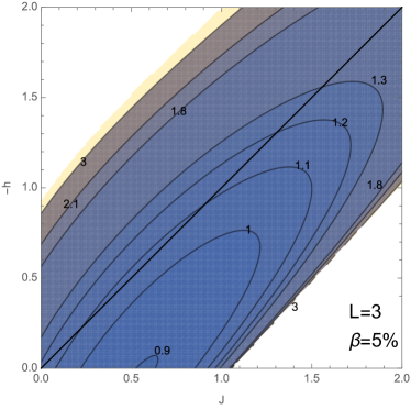
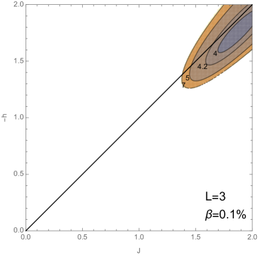
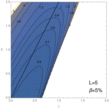
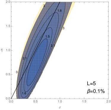
Figure 6: Time needed to reach a certain sensitivity as a function of the coupling coefficient $J$ and minus the external field $-h=\log\frac{K_{d}}{c}$. The solid line indicates $-h=J(L-1)/2$ which corresponds to the values of the concentration set at the transition point that were used to draw figure 5. The top figures refer to the case with $L=3$ and the bottom ones to $L=5$. For each value the concentration change to be detected is such that $c^{\prime}/c=0.9$ corresponding to $\delta h=-0.1$. Time is expressed in units of $k_{u}^{-1}$.

This is the value for which the system is most sensitive to concentration changes. In order to extend our reasonings to cases in which the system is not optimally tuned, let us consider how the detection time depends on the reference concentration (or, equivalently, on the dissociation constant). The results are reported in fig. 6. For each level of concentration it is possible to determine the range of cooperativity that allows for a given sensitivity and the coupling intensity $J$ that reaches it in the shortest time. The fastest detections are achieved for combinations of concentration and coupling such that the system is close to the transition point but higher concentrations are favored. This reflects the fact that the concentration change has to be within the dynamic range of the receptor and that higher concentrations imply a faster ligand binding consequently accelerating the dynamics.

3.3 Non-homogeneous coupling strength and ligand affinity across the receptors.

In the previous sections we have considered the case in which each receptor has the same coupling strength and ligand affinity. In general, it is possible that different receptors have different $J$ and $K_{d}$. Let us consider the case in which the $J$ and $K_{d}$ of each receptor are drawn from a distribution $\rho(J,K_{d})$. If the number of receptors $N$ is large enough so that each value of the pair $J,K_{d}$ is sampled several times we can still exploit Stein’s lemma for each receptors subpopulation. The overall miss probability is then an average over the different receptors subpopulations reading

$$\log\beta\sim-N\int\rho(J,K_{d})\,D_{KL}\left(p_{eq}^{c}(J,K_{d})||p_{t}^{c^{\prime}}(J,K_{d})\right)dJ\,dK_{d}\,.$$ (34)

As a specific example, consider the case where the receptors are a mixture of two different subpopulations characterized by two different couplings $J_{w}$ and $J_{s}$ with the respective $K_{d}$ tuned as $K_{d}(J)=K_{d}^{(0)}e^{\frac{J}{2}(L-1)}$ so that the transition point is for both populations at $c_{1/2}=K_{d}^{(0)}$.

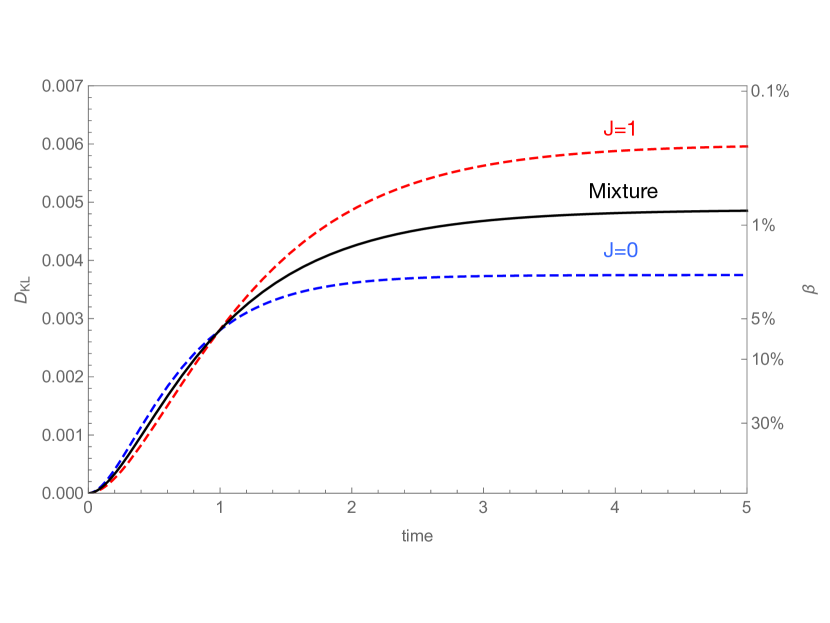
Figure 7: In the case of non-homogeneous coupling strength across the receptors the miss probability is given by a linear combination of the various couplings. The plot refers to the case in which a receptor is cooperative with $J=1$ with probability $q=1/2$ and is noncooperative with probability $1-q=1/2$ with $L=3$ and $c^{\prime}=c\,e^{-0.1}$. Time is expressed in units of $\left(k_{u}\sqrt{c^{\prime}/c_{1/2}}\right)^{-1}$.

Let us denote the probability of drawing the strongly cooperative ($J_{s}$) receptor as $q$ so that we have, on average $Nq$ strongly cooperative receptors. The miss probability then obeys

$$\log\beta\sim-N\left[qD_{KL}\left(p_{eq}^{c}(J_{s})||p_{t}^{c^{\prime}}(J_{s})\right)+(1-q)D_{KL}\left(p_{eq}^{c}(J_{w})||p_{t}^{c^{\prime}}(J_{w})\right)\right]$$ (35)

resulting in a linear combination of the two Kullback-Leibler divergences. By varying the parameter $q$ from $0$ to $1$ the curve smoothly varies between the weakly and the strongly cooperative cases. In general, such mixture of receptors displays a faster initial response compared to the strongly cooperative case and a higher asymptotic precision with respect to the weakly cooperative case (see fig 7). This allows for intermediate behaviors which can be tuned to satisfy different requirements by changing the sizes of the subpopulations.

4 Conclusions and discussion

We have studied the problem of detecting a change in concentration of a ligand by means of a pool of receptors. To investigate the detection performance we have addressed the problem in terms of hypothesis testing making use of the instantaneous occupancy. We have focused on the probability of missing the detection of a change that actually occurred and employed it as a measure of the quality of the sensing system. With this formalism we have considered the influence of cooperativity on the sensing performance. We have identified a twofold effect of cooperativity: a markedly improved sensitivity in the long time limit and a significant slowing down of the receptors dynamics. This is consistent with the findings of Ref. skoge11 in which the sensing performance of locally cooperative receptors was considered in terms of the precision with which they are able to determine a concentration change by time averaging their history. We stress here that both the higher asymptotic sensitivity and the slowing down are separately relevant. Most notably, cooperativity enables to detect changes with sensitivities that are not attainable by noncooperative receptors. When considering the time from the concentration change needed before the instantaneous receptor occupancy state can provide a given detection sensitivity, the two effects of cooperativity trade off. In the framework adopted by the authors of skoge11 , the effect of the slowdown due to cooperativity on the time averaging procedure dominates the additional sensitivity and the authors concluded that noncooperative receptors perform better than cooperative ones. On the contrary, we have seen that, casting the detection problem in terms of hypothesis testing by means of the instantaneous occupancy of a pool of receptors, cooperativity can be beneficial. We have found that there is an optimal degree of cooperativity which depends on the required sensitivity level and on the number of binding sites present in each receptor. At given number of binding sites we can identify three general scenarios depending on the required detection power. For hard detections the system must be cooperative and the desired sensitivity is reached earlier at finite but large levels of cooperativity. For intermediate cases the system can achieve the needed statistical power by noncooperative binding sites but moderately cooperative receptors are faster at approaching it. Easy detections are performed more rapidly by noncooperative receptors.

It is interesting to consider how the cell’s detection ability scales with the numbers of receptors and binding sites. For noncooperative binding sites the probability of missing the detection decreases exponentially with the total number of binding sites present in all the receptors $NL$. We have shown that for cooperative receptors in the long-time limit the exponential decrease is more marked and in the infinite coupling limit for small concentration changes depends quadratically on the number of binding sites present in each receptor: $NL^{2}$. Since it is costly to produce proteins (see Refs.dekel05 ; govern14pnas ) sensing mechanisms that improve the performances without increasing the number of required components may represent an advantage. The different scaling in $N$ and $L$ can then impact on how to invest the limited resources favoring either solutions involving few receptors with many binding sites or the opposite. The characterisation of the ensuing trade-offs is an issue that surely deserves further study in the near future.

References

- (1) Aquino, G., Clausznitzer, D., Tollis, S., and Endres, R. G.: Optimal receptor-cluster size determined by intrinsic and extrinsic noise. Physical Review E, 83(2), 021914. (2011).
- (2) Aquino, G., Tweedy, L., Heinrich, D., Endres, R. G.: Memory improves precision of cell sensing in fluctuating environments. Scientific reports, 4. (2014).
- (3) Barato, A. C., Hartich, D., Seifert, U.: Information-theoretic vs. thermodynamic entropy production in autonomous sensory networks. Phys. Rev. E 87, 042104 (2013).
- (4) Barato, A. C., Hartich, D., Seifert, U.: Efficiency of cellular information processing. New J. Phys. 16 103024 (2014).
- (5) Barato, A. C., Seifert, U.: Thermodynamic uncertainty relation for biomolecular processes. Phys. Rev. Lett., 114(15), 158101. (2015).
- (6) Berg, H., Purcell, E.: Physics of chemoreception. Biophys. J. 20, 193 (1977).
- (7) Bialek, W., Biophysics: searching for principles. Princeton University Press, (2012).
- (8) Bialek, W., Setayeshgar, S.: Physical limits to biochemical signaling. Proc. Natl. Acad. Sci. USA 102, 10040 (2005).
- (9) Bialek, W., Setayeshgar, S.: Cooperativity, sensitivity, and noise in biochemical signaling. Phys. Rev. Lett., 100(25), 258101. (2008).
- (10) Bowsher, C. G., Swain, P. S.: Identifying sources of variation and the flow of information in biochemical networks. Proc. Natl. Acad. Sci. USA, 109(20), E1320-E1328. (2012).
- (11) Bowsher, C. G., Swain, P. S.: Environmental sensing, information transfer, and cellular decision-making. Curr. Opin. Biotech, 28, 149-155. (2014)
- (12) Cover, T. M., Thomas, J. A., Elements of information theory. John Wiley & Sons. (2012).
- (13) Cheong, R., Rhee, A., Wang, C. J., Nemenman, I., Levchenko, A.: Information transduction capacity of noisy biochemical signaling networks. Science, 334(6054), 354-358 (2011).
- (14) Diana, G., Esposito, M.,:Mutual entropy production in bipartite systems J. Stat. Mech.(4), P04010 (2014).
- (15) Dekel, E., Alon, U.: Optimality and evolutionary tuning of the expression level of a protein. Nature, 436(7050), 588-592. (2005).
- (16) Dubuis, J. O., Tkac̆ik, G., Wieschaus, E. F., Gregor, T., Bialek, W.: Positional information, in bits. Proc. Natl. Acad. Sci. USA, 110(41), 16301-16308. (2013).
- (17) Endres, R.G., Wingreen, N. S.: Maximum likelihood and the single receptor. Phys. Rev. Lett. , 103(15), 158101, (2009).
- (18) Govern, C.C., ten Wolde, P.R.: Fundamental limits on sensing chemical concentrations with linear biochemical networks. Phys. Rev. Lett. 109:218103 (2012).
- (19) Govern, C.C., ten Wolde, P.R.: Optimal resource allocation in cellular sensing systems Proc. Natl.Acad. Sci. USA 111 17486–91 (2014).
- (20) Govern, C.C., ten Wolde, P.R.: Energy dissipation and noise correlations in biochemical sensing. Phys. Rev. Lett., 113(25), 258102. (2014).
- (21) Hartich, D., Barato, A. C., Seifert, U.: Nonequilibrium sensing and its analogy to kinetic proofreading. New J. Phys., 17(5), 055026. (2015).
- (22) Hill, T. L.: Cooperativity Theory in Biochemistry: Steady-State and Equilibrium Systems. p. 66. Springer- Verlag: New York, NY. (1985).
- (23) Hu, B., Chen, W., Rappel, W. J., Levine, H.: Physical limits on cellular sensing of spatial gradients. Phys. Rev. Lett. , 105(4), 048104 (2010).
- (24) Kaizu, K., de Ronde, W., Paijmans, J., Takahashi, K., Tostevin, F., ten Wolde, P. R.: The berg-purcell limit revisited. Biophys. J., 106(4), 976-985. (2014).
- (25) Kobayashi, T. J.: Implementation of dynamic Bayesian decision making by intracellular kinetics. Phys. Rev. Lett., 104(22), 228104 (2010).
- (26) Lan, G., Sartori, P., Neumann, S., Sourjik V., and Tu, Y., The energy-speed-accuracy trade-off in sensory adaptation. Nat. Phys., 8(5), 422-428, (2012).
- (27) Lang, A. H., Fisher, C. K., Mora T., Mehta, P.: Thermodynamics of statistical inference by cells Phys. Rev. Lett. 113, 148103 (2014).
- (28) Levchenko, A., Nemenman, I.: Cellular noise and information transmission. Curr. Opin. Biotech., 28, 156-164 (2014).
- (29) Mancini, F., Wiggins, C. H., Marsili, M., Walczak, A. M. Time-dependent information transmission in a model regulatory circuit. Phys. Rev. E, 88(2), 022708. (2013).
- (30) Mancini, F., Marsili, M., Walczak, A. M.: Trade-offs in delayed information transmission in biochemical networks. arXiv preprint arXiv:1504.03637. (2015).
- (31) Martins, B. M., Swain, P. S.: Trade-offs and constraints in allosteric sensing. PLoS Comput. Biol. 7, e1002261. (2011).
- (32) Marzen, S., Garcia, H. G., Phillips, R. Statistical mechanics of Monod–Wyman–Changeux (MWC) models. J. Mol. Biol., 425(9), 1433-1460. (2013).
- (33) Mehta, P., Schwab, D.: Energetic costs of cellular computation. Proc. Natl. Acad. Sci. USA 109, 17978 (2012).
- (34) Mora, T., Wingreen, N. S.: Limits of sensing temporal concentration changes by single cells. Phys. Rev. Lett., 104(24), 248101. (2010).
- (35) Mugler, A., Tostevin, F., ten Wolde, P. R.: Spatial partitioning improves the reliability of biochemical signaling. Proc. Natl. Acad. Sci. USA, 110(15), 5927-5932. (2013).
- (36) Murugan, A., Huse, D. A., Leibler, S., Speed, dissipation, and error in kinetic proofreading. Proc. Natl. Acad. Sci. USA 109(30):12034-9. doi: 10.1073/Proc. Natl. Acad. Sci. USA.1119911109. (2012).
- (37) Ouldridge, T., Govern, C. , ten Wolde, P. R.: On the connection between computational and biochemical measurement. arXiv preprint arXiv:1503.00909. (2015).
- (38) Phillips, R., Kondev, J., Theriot, J., Garcia, H. Physical biology of the cell. Garland Science. (2012).
- (39) Rieckh, G., Tkac̆ik, G.: Noise and information transmission in promoters with multiple internal states. Biophys. J., 106(5), 1194-1204. (2014).
- (40) Qian, H., Reluga, T. C.: Nonequilibrium Thermodynamics and Nonlinear Kinetics in a Cellular Signaling Switch. Phys. Rev. Lett. 94 028101 (2005).
- (41) Qian, H.: Reducing intrinsic biochemical noise in cells and its thermodynamic limit. J. Mol. Biol., 362(3), 387-392. (2006).
- (42) Rappel, W. J., Levine, H. Receptor noise and directional sensing in eukaryotic chemotaxis. Phys. Rev. Lett., 100(22), 228101. (2008).
- (43) Sartori, P., Pigolotti, S.: Kinetic versus Energetic Discrimination in Biological Copying Phys. Rev. Lett. 110, 188101 (2013).
- (44) Sartori, P., Granger, L., Lee, C. F., Horowitz, J. M.: Thermodynamic costs of information processing in sensory adaptation. PLos Comput. Biol., 10(12), e1003974. (2014).
- (45) Selimkhanov, J., Taylor, B., Yao, J., Pilko, A., Albeck, J., Hoffmann, A., Tsimring, L., Wollman, R.: Accurate information transmission through dynamic biochemical signaling networks. Science, 346(6215), 1370-1373 (2014).
- (46) Sevier, S. A., Levine, H.: Properties of Cooperatively Induced Phases in Sensing Models. Phys. Rev. E, 91(5), 052707 (2015).
- (47) Siggia, E. D., Vergassola, M.: Decisions on the fly in cellular sensory systems. Proc. Natl. Acad. Sci. USA , 110(39), E3704-E3712. (2013).
- (48) Skoge, M., Meir, Y., Wingreen, N. S.: Dynamics of cooperativity in chemical sensing among cell-surface receptors. Phys. Rev. Lett., 107(17), 178101 (2011).
- (49) Skoge, M., Naqvi, S., Meir Y., Wingreen N. S.: Chemical Sensing by Nonequilibrium Cooperative Receptors Phys. Rev. Lett. 110 248102 (2013).
- (50) Sun, J., Grabe, M.: Cooperativity Can Enhance Cellular Signal Detection. arXiv preprint arXiv:1401.3262. (2014).
- (51) Tănase-Nicola, S., Warren, P. B., ten Wolde, P. R.: Signal detection, modularity, and the correlation between extrinsic and intrinsic noise in biochemical networks. Phys. Rev. Lett., 97(6), 068102. (2006).
- (52) Tkac̆ik, G., Callan, J. C. G. Bialek, W.: Information flow and optimization in transcriptional regulation. Proc. Natl. Acad. Sci. 105, 12265–12270. (2008).
- (53) Tkac̆ik, G., Walczak, A. M., Bialek, W: Optimizing information flow in small genetic networks. Phys. Rev. Lett. 80, 031920, (2009).
- (54) Tkac̆ik, G., Walczak, A. M.: Information transmission in genetic regulatory networks: a review. J. Phys.-Condens. Matt., 23(15), 153102. (2011)
- (55) Tkac̆ik, G., Walczak, A. M., Bialek, W.: Optimizing information flow in small genetic networks. III. A self-interacting gene. Phys. Rev. E, 85(4), 041903. (2012).
- (56) Tostevin, F., Ten Wolde, P. R.: Mutual information between input and output trajectories of biochemical networks. Phys. Rev. Lett., 102(21), 218101. (2009).
- (57) Tu, Y.: The nonequilibrium mechanism for ultrasensitivity in a biological switch: Sensing by Maxwell’s demons. Proc. Natl. Acad. Sci. USA 105, 11737–11741 (2008).
- (58) Uda, S., Saito, T. H., Kudo, T., Kokaji, T., Tsuchiya, T., Kubota, H., Komori, Y., Ozaki, Y., Kuroda, S.: Robustness and compensation of information transmission of signaling pathways. Science, 341(6145), 558-561. (2013).
- (59) Voliotis, M., Perrett, R. M., McWilliams, C., McArdle, C. A., Bowsher, C. G.: Information transfer by leaky, heterogeneous, protein kinase signaling systems. Proc. Natl. Acad. Sci. USA, 111(3), E326-E333. (2014).
- (60) Walczak, A. M., Tkac̆ik, G., Bialek, W.: Optimizing information flow in small genetic networks. II. Feed-forward interactions. Phys. Rev. E, 81(4), 041905. (2010).
- (61) Ziv, E., Nemenman, I., Wiggins, C. H: Optimal signal processing in small stochastic biochemical networks. PLoS One, 2(10), e1077. (2007).