Influence of Rough and Smooth Walls on Macroscale Flows in Tumblers

Abstract

Walls in discrete element method (DEM) simulations of granular flows are sometimes modeled as a closely packed monolayer of fixed particles, resulting in a rough wall rather than a geometrically smooth wall. An implicit assumption is that the resulting rough wall differs from a smooth wall only locally at the particle scale. Here we test this assumption by considering the impact of the wall roughness at the periphery of the flowing layer on the flow of monodisperse particles in a rotating spherical tumbler. We find that varying the wall roughness significantly alters average particle trajectories even far from the wall. Rough walls induce greater poleward axial drift of particles near the flowing layer surface, but decrease the curvature of the trajectories. Increasing the volume fill level in the tumbler has little effect on the axial drift for rough walls, but increases the drift while reducing curvature of the particle trajectories for smooth walls. The mechanism for these effects is related to the degree of local slip at the bounding wall, which alters the flowing layer thickness near the walls, affecting the particle trajectories even far from the walls near the equator of the tumbler. Thus, the proper choice of wall conditions is important in the accurate simulation of granular flows, even far from the bounding wall.

I Introduction

Discrete element method (DEM) simulations have been used extensively to study the motion of granular materials in many situations as a predictive tool as well as to obtain data that is otherwise inaccessible experimentally. In the method each particle’s motion is governed by Newton’s laws: the goal is to compute the evolution of linear and angular momentum of every individual particle by using appropriate contact force models SchaferDippel96 ; Ristow00 ; CundallStrack79 . While early DEM simulations could manage systems with only a few hundred to tens of thousands of particles Shoichi98 ; HirshfeldRapaport01 ; Ristow94 ; McCarthyOttino98 ; MoakherShinbrot00 ; YangZou03 ; YamaneNakagawa98 , simulating millions of particles is now practical with advances in computer technology.

As with many simulation approaches, one of the key aspects is the implementation of boundary conditions. Two types of wall boundary conditions can be implemented in DEM simulations for the calculation of the collision force between mobile granular particles and the walls: 1) geometrically smooth surfaces, which are assumed to have infinite mass and a specified radius of curvature (infinite for planar walls) (for example, see ChenLueptow11 ; MoakherShinbrot00 ; TaberletLosert04 ; Rapaport02 ; TaberletNewey06 ); and 2) a geometrically rough surface made up of a closely packed monolayer of fixed particles conforming to the geometry of the wall surface (for example, see DaCruzEmam05 ; McCarthyOttino98 ; PoschelBuchholtz95 ; JuarezChen11 ; BertrandLeclaire05 ). The latter approach, often called a “rough wall,” is easy to implement because interactions between mobile particles and immobile wall particles are modeled in almost exactly the same way as between pairs of mobile particles. The only difference is that the wall particles remain fixed in their wall position. An implicit assumption is typically that a rough wall differs from a smooth wall only locally at the particle scale or perhaps through the thickness of the flowing layer, which is typically $O(10)$ particles thick PignatelLueptow12 , but is unlikely to have a global effect on the flow, particularly far from the wall. Likewise, it is often implicitly assumed that a rough wall is similar to a smooth wall, but one with a very high coefficient of friction.

In this paper, we examine the impact of the wall boundary condition on the flow using the system of monodisperse particles in a partially-filled spherical tumbler rotating with angular velocity $\omega$ about a horizontal axis (Fig. 1).

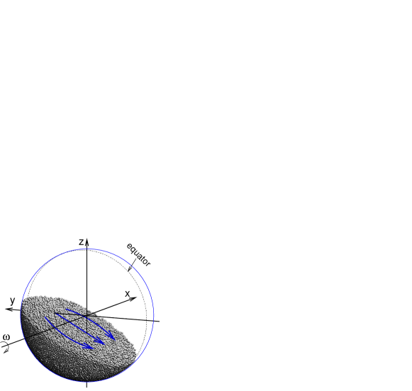
Figure 1: (Color online) 14 cm diameter spherical tumbler filled at 30% with 2 mm particles. The blue arrows at the free surface show the direction of the flow. $x$ is the polar axis, $y$ and $z$ are in the equatorial plane.

We consider the situation where the free surface is essentially flat and continuously flowing. In this regime, the surface of the flowing layer maintains a dynamic angle of repose $\beta$ with respect to horizontal, which depends on the frictional properties and diameter $d$ of the particles and the rotational speed of the tumbler TaberletRichard03 ; duPontGondret03 ; PignatelLueptow12 ; MeierLueptow07 .

In spherical tumblers, it has been shown that monodisperse particles slowly drift axially toward the pole near the surface of the flowing layer, while they drift axially toward the equator deep in the flowing layer with an axis of symmetry at the equator ZamanDOrtona13 .

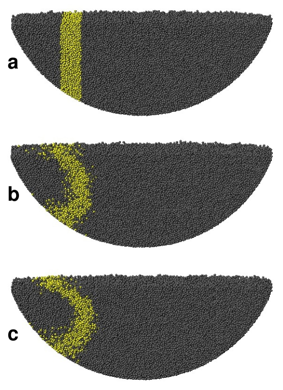
Figure 2: (Color online) Axial deformation of a vertical band of 1 mm colored particles in a 14 cm diameter spherical tumbler filled at 30% and rotating at 15 rpm. (a) The band is initially placed between -4 cm and -3 cm from the equator. After rotation of the tumbler about a horizontal axis in the plane of the page so that particles have made two circulations through the flowing layer the band is deformed. The wall is (b) perfectly smooth or (c) rough, made of 1 mm particles. The front half of the bed of particles has been removed in order to view a cross-section through the bed of particles.

For example, consider the deformation of an initially vertical band of colored particles in a 30% full spherical tumbler shown in Fig. 2(a). In this figure, the axis of rotation is horizontal, and the front half of the bed of 1 mm diameter particles has been removed to view a cross-section of the particles. In Fig. 2, after 2 circulations of particles through the flowing layer, the initially vertical band of colored particles is more slightly deformed in the case of a rough wall (1 mm diameter particles forming the wall) in Fig. 2(c) than in the case of a smooth wall in Fig. 2(b). To generate these images, it was necessary to choose a time corresponding to an integer number of circulations of particles through the flowing layer so that particles that were in the static bed return to the static bed and particles in flowing layer return to the flowing layer. To do this, we measured the average recirculation time of all particles: 2.14 s for the smooth case and 2.04 s for the rough case. This recirculation time difference does not come from slip between the smooth wall and the granular media in solid body rotation. This difference is instead due to a global modification of the flow due to the wall roughness.

The deformation of the colored band comes about from asymmetries in the curvature of particle trajectories in the flowing layer that result in poleward drift near the free surface ZamanDOrtona13 . Mass conservation requires equator-directed drift deeper in the flowing layer. Although our previous study ZamanDOrtona13 indicated that the axial drift occurs for both smooth and rough walls, the degree of axial drift was not studied in detail. It is the unexpectedly strong influence of wall roughness on deformation of a labeled band in Fig. 2, that we examine primarily through simulations in order to better understand the impact of wall boundary conditions in DEM simulations and experiments.

By way of background, the wall roughness has been shown to affect the flow of granular media in cases like chute flows and shear cell flows. For instance, the roughness of the bottom wall in chute flow has an impact on velocity GoujonThomas03 ; Augenstein78 ; ThorntonWeinhart12 ; WeinhartThornton12 and velocity profile Ancey01 . In planar shear flows Campbell93a ; Campbell93b , a smooth wall results in a slip velocity at the wall and large velocity gradients near the wall, whereas a rough wall results in no slip velocity and a nearly uniform velocity gradients. In both chute flow and planar shear flow, the impact of wall roughness on the flowing layer in the immediate vicinity is quite direct. The frictional effects at the wall alter the local shear rate at the wall, which propagates through the thickness of the entire flowing layer to affect the velocity profile. For granular flows in pipes, wall roughness can prevent clogging and jamming regimes by deflecting particles toward the center of the pipe VerbuchelnParteli15 . The case studied here, the wall only contacts the flowing layer at its circular periphery, not at the bottom of the flowing layer, which is in contact with the underlying bed of particles that is rotating in solid body motion with the tumbler. Thus, the impact of the wall roughness is quite different and much less direct.

II DEM Simulations

For the DEM simulations, a standard linear-spring and viscous damper force model ChenLueptow08 ; SchaferDippel96 ; Ristow00 ; CundallStrack79 was used to calculate the normal force between two contacting particles:
$F_{n}^{ij}=[k_{n}\delta-2\gamma_{n}m_{\rm eff}(V_{ij}\cdot\hat{r}_{ij})]\hat{r}_{ij}$, where $\delta$ and $V_{ij}$ are the particle overlap and the relative velocity $(V_{i}-V_{j})$ of contacting particles $i$ and $j$ respectively; $\hat{r}_{ij}$ is the unit vector in the direction between particles $i$ and $j$; $m_{\rm eff}=m_{i}m_{j}/(m_{i}+m_{j})$ is the reduced mass of the two particles; $k_{n}=m_{\rm eff}[(\pi/\Delta t)^{2}+\gamma^{2}_{n}]$ is the normal stiffness and $\gamma_{n}=\ln e/\Delta t$ is the normal damping, where $\Delta t$ is the collision time and $e$ is the restitution coefficient ChenLueptow08 ; Ristow00 . A standard tangential force model SchaferDippel96 ; CundallStrack79 with elasticity was implemented: $F^{t}_{ij}=-\min(|\mu F^{n}_{ij}|,|k_{s}\zeta|){\rm sgn}(V^{s}_{ij})$, where $V^{s}_{ij}$ is the relative tangential velocity of two particles Rapaport02 , $k_{s}$ is the tangential stiffness, $\mu$ the Coulomb friction coefficient and $\zeta(t)=\int^{t}_{t_{0}}V^{s}_{ij}(t^{\prime})dt^{\prime}$ is the net tangential displacement after contact is first established at time $t=t_{0}$. The velocity-Verlet algorithm Ristow00 ; AllenTildesley02 was used to update the position, orientation, and linear and angular velocities of each particle. Tumbler walls were modeled as both smooth surfaces (smooth walls) and as a monolayer of fixed particles that are just touching with no overlap between particles (rough walls). The number of particles that comprise the wall ranged from 2300 in the case of a wall of 6 mm particles to 1.13 million for a wall of 0.25 mm particles. All wall conditions have infinite mass for calculation of the collision force between the tumbling particles and the wall.

The spherical tumbler of radius $R=D/2=7$ cm was filled to volume fraction $f$ with monodisperse $d=1$ mm to 4 mm particles, though most simulations used $d=2$ mm particles; gravitational acceleration was $g$ = 9.81 m s^-2; particle properties correspond to cellulose acetate: density $\rho=$ 1308 kg m^-3, restitution coefficient $e$ = 0.87 DrakeShreve86 ; FoersterLouge94 ; SchaferDippel96 . The particles were initially randomly distributed in the tumbler with a total of about $5\times 10^{4}$ particles in a typical simulation. To avoid a close-packed structure, the particles had a uniform size distribution ranging from 0.95$d$ to 1.05$d$. Unless otherwise indicated, the friction coefficients between particles and between particles and walls was set to $\mu=0.7$. The collision time was $\Delta t=10^{-4}$ s, consistent with previous simulations TaberletNewey06 ; ChenLueptow11 ; ZamanDOrtona13 and sufficient for modeling hard spheres Ristow00 ; Campbell02 ; SilbertGrest07 . These parameters correspond to a stiffness coefficient $k_{n}=7.32\times 10^{4}$ (N m^-1) and a damping coefficient $\gamma_{n}=0.206$ kg s^-1 SchaferDippel96 . The integration time step was $\Delta t/50=2\times 10^{-6}$ s to meet the requirement of numerical stability Ristow00 . The rotational speed of the tumbler is $\omega=15$ rpm in most cases, consistent with previous studies of spherical tumbler flow ChenLueptow09 and chosen such that, for this system size, the flow is continuous, dense, and with a flat free surface rather than discrete avalanches at very low rotation speeds or a curved free surface at higher rotation speeds. A few cases at other rotational speeds were studied ($\omega=2.5$ to 30 rpm), all in the continuous flow regime. The free surface remains flat up to 20 rpm and becomes slightly S-shaped at 30 rpm.

III Results

III.1 Deformation of a vertical band

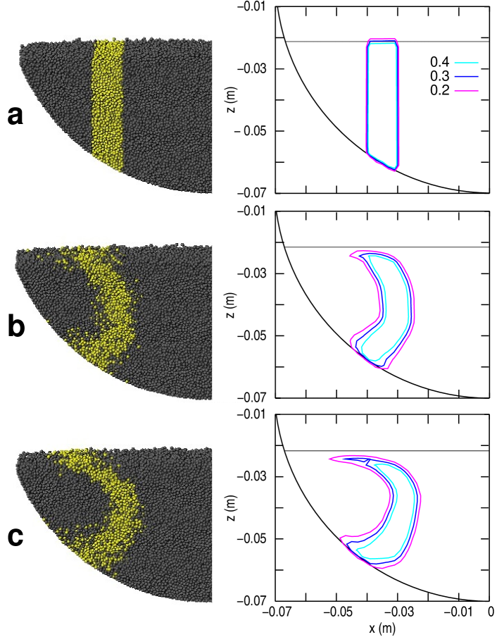
Figure 3: (Color online) Deformation of a vertical band of 1 mm colored particles in a 14 cm diameter tumbler filled at 30% and rotating at 15 rpm. The axis of rotation is horizontal at $z=0$ and in the plane of the page, the equator is at $x=0$, and gravity is down. The image shows the back half of the particle bed after the front half and right half are removed. Left: The initial band (a) and the deformed bands as shown in Fig 2. Right: the corresponding compacity contour levels of colored particles to show more accurately the band deformation difference for smooth (b) and 1 mm rough (c) cases. The horizontal line represents the fill level.

Figure 3 shows the band deformation, like Fig. 2, with the corresponding concentration map of the colored particles. The contours correspond to iso-volume concentration, or iso-compacity. The maximum compacity is about 0.6, but the boundaries of the colored particles correspond most closely to contours ranging from 0.2 to 0.4. Using this compacity map, the deformation of the band is quite clear. After just two passes of particles through the flowing layer, the deformation of the initially vertical band, with the 1 mm rough wall results in more deformation than the band in a tumbler with a smooth wall.

Figure 4: (Color online) Deformation of a vertical band of 2 mm colored particles in a 14 cm diameter tumbler filled at 30% and rotating at 15 rpm around a horizontal axis at $z=0$. The band is initially placed between $x=-4$ cm and $x=-3$ cm from the equator (dashed vertical lines). The roughnesses of the walls range from smooth to 6 mm particles. The iso-compacity contours are measured after two circulations of the particles through the flowing layer. The horizontal line represents the fill level.

Similar results also occur for larger flowing particles. Figure 4 shows the deformation of a band of colored 2 mm particles in a 14 cm spherical tumbler filled to 30% by volume with varying wall roughness so that the innermost surfaces of the wall particles are at a radius $R=7$ cm. From perfectly smooth to a 2 mm rough wall, the band becomes increasingly more deformed, though the roughness does not modify the band deformation much from 2 mm to 6 mm wall roughness.

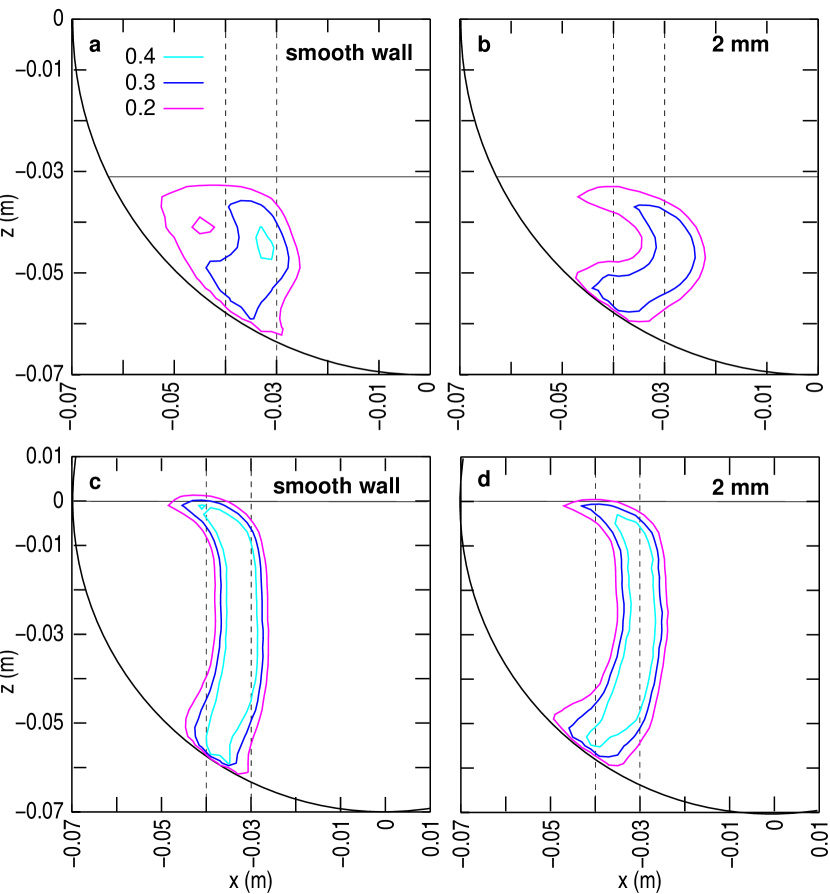
Figure 5: (Color online) Deformation of a vertical band of 2 mm colored particles in a 14 cm diameter tumbler filled at 20% (a and b) or 50% (c and d) and rotating at 15 rpm based on iso-compacity contours. The band is initially placed between $x=-4$ cm and $x=-3$ cm from the equator (vertical dashed lines). Two roughnesses are shown: smooth wall and 2 mm particles. The horizontal line indicates the fill level.

Similar results occur for 20% and 50% full tumblers as shown in Fig. 5. For each case, only iso-compacity contours for smooth and 2 mm rough walls have been plotted, but we have also simulated wall roughnesses of 0.5, 1, 1.5, and 3 mm with consistent results. In a tumbler filled to 20%, there is a significant difference in the deformation of the colored band between the smooth and rough cases. For the 50% full tumbler, the band of colored particles is less deformed. In addition, the difference in the band deformation between the smooth and rough walls is smaller for the 50% fill volume indicating that the influence of the wall roughness increases for smaller fill fractions.

III.2 Mean trajectories

To investigate the mechanism behind the results described above, we consider 2 mm particles in a 30% full 14 cm tumbler with smooth and rough walls.

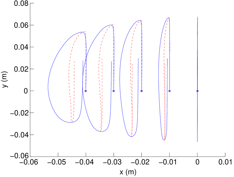
Figure 6: (Color online) Comparison (top view) of the mean trajectories (initially 2 mm above the sphere wall) for 2 mm particles starting from the same points in the smooth wall (blue continuous lines) and in the rough (2 mm particles) wall (red dashed lines) in a sphere filled at 30%. The horizontal axis of rotation is at $y=0$.

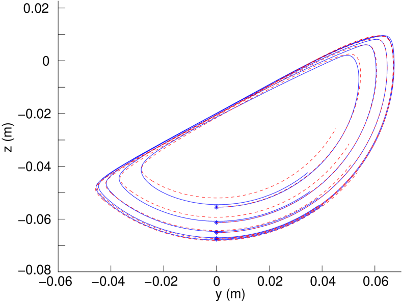
Figure 7: (Color online) Comparison (side view) of the mean trajectories (initially 2 mm above the sphere wall) for 2 mm particles starting from the same points in the smooth wall (blue continuous lines) and in the rough (2 mm particles) wall (red dashed lines) in a sphere filled at 30%. The axis of rotation is perpendicular to the page at $(y,z)=(0,0)$.

Figures 6 and 7 show average trajectories of particles constructed by integrating the mean velocity field using a second order Runge-Kutta scheme ZamanDOrtona13 . The two trajectories in each pair correspond to smooth and 2 mm rough walls. The trajectories are shown for several different initial axial positions in the tumbler, where $x=0$ corresponds to the equator. Both trajectories in a pair start at the same point (indicated by a star) in the fixed bed, initially 2 mm away from the sphere wall and below the axis of rotation (Fig. 7). In Fig. 6, the initial vertical portion of the trajectory corresponds to motion in the fixed bed as the tumbler rotates. Particles enter the flowing layer at the topmost part of the trajectory and follow a curved path in the flowing layer until they re-enter the fixed bed at the bottommost part of the trajectory, again following a vertical path in the figure when in solid body rotation. The paths are viewed looking downward along the gravity vector, so the flowing layer surface is not perpendicular to the line along which the trajectories are viewed.

Two results are clearly evident in Fig. 6. First, the trajectories in the flowing layer for both cases are curved, with the curvature for smooth walls much greater than that for rough walls. This curvature is negligible at the equator (at $x=0$, which is a plane of symmetry) and increases moving toward the poles, consistent with previous results in smooth-walled tumblers ChenLueptow10 ; ZamanDOrtona13 . Second, the trajectories for the smooth-walled tumbler are nearly closed, displaying only a very small amount of poleward drift with each pass through the flowing layer. On the other hand, the poleward drift for the rough-walled tumbler is much larger. For that reason, the band undergoes more deformation in the rough case (Figs. 3-5). In both cases, the drift increases toward the poles, consistent with previous results for smooth tumblers ZamanDOrtona13 . Thus, two quantities can be used to characterize the trajectories: the “displacement”, which is the maximum axial displacement of the trajectory from its starting point that occurs at any point during one trajectory circulation through the flowing layer, and the poleward “drift”, which is the net axial displacement of the trajectory after one trajectory circulation. Although the displacement and drift differ substantially for smooth and 2 mm rough walls, Fig. 7 shows there is little difference in the trajectories viewed along the axis of rotation.

While previous simulations and experiments match reasonably well when considering axial drift of particles in spherical tumblers ZamanDOrtona13 , we have attempted to directly validate the simulation results in Fig. 6 experimentally using tracer particles in a tumbler under similar conditions. However, it is quite difficult to obtain quantitative experimental results. Several problems occur. First, visualizing the flow and tracking tracer particles in a rough-walled tumbler is difficult, because the rough wall makes the particles in the tumbler challenging to access via optical means. Second, the inherent collisional diffusion makes it difficult to obtain displacement or drift data because of the statistical variation in the tracer particle location, both axially and depthwise. Thus, obtaining highly-resolved experimental mean trajectories of tracer particles is challenging. To overcome these problems, we have used an X-ray system to track the location of a single X-ray opaque tracer particle in a 14 cm spherical tumbler that is 30% filled by volume with 2 mm spherical glass particles rotating at 6.5 rpm, the maximum speed for which a tracer particle can be accurately tracked. The tracer particle is 3 mm, so it remains near the surface of the flowing layer, but it still follows the general trajectory of the 2 mm particles based on direct visual observation in the smooth tumbler, an approach we have used successfully in the past ZamanDOrtona13 . The tracer consists of a small ball of lead solder enclosed in a plastic shell such that the overall density of the tracer matches that of the glass particles.

Figure 8: (Color online) Individual trajectory segments (top view) from experiment of a 3 mm tracer particle in a bed of 2 mm particles in a (a) smooth wall and in a (b) rough (2 mm particles) wall spherical tumbler filled at 30%. Each trajectory segment consists of one circulation through the fixed bed and the flowing layer with a starting positions of $-3.5$ cm $\leq x\leq-2.5$ cm. The starting position (star) of each trajectory was shifted to $x=−3$  cm to make it easier to distinguish the drift. The endpoint of each trajectory is marked with a square box. Note that the solid body portion of the trajectory appears curved due to the inherent depthwise geometric magnification in the X-ray image.

The experimental results are shown in Fig. 8 for 7 randomly selected particle trajectories for each case, all starting with an axial position in the range $-3.5$ cm $\leq x\leq-2.5$ cm and directly below the axis of rotation in the fixed bed, but shifted axially in the figure to the same starting location. The poleward drift in a smooth wall tumbler is close to zero in all cases (Fig. 8(a), noting the trajectory endpoints marked with a square box), while it is up to 0.7 cm in the rough wall tumbler (Fig. 8(b)). While these results are limited in scope, they are consistent with the simulation results in Fig. 6 and our previous results for the amount of axial drift in a tumbler with smooth walls ZamanDOrtona13 . The curvature is less in both cases than occurs in the simulations, perhaps due to different particles characteristics. Nevertheless, these experiments clearly validate the simulation results in spite of substantial variation in the trajectories due to collisional diffusion. That is, curvature of the trajectories, and hence displacement, is larger for smooth tumbler walls, while axial drift is greater for rough tumbler walls. Due to the difficulty in performing these experiments, we focus on simulation results in the remainder of the paper. Note however that we performed DEM simulations to match the conditions in the experiments (3 mm tracer). These simulation results are consistent with the experiments and with DEM results tracking a single 2 mm (instead of 3 mm) tracer particle, thus demonstrating that using a 3 mm tracer with otherwise 2 mm particles is a valid experimental approach.

Similar DEM simulation results occur for 2 mm particles in 20% and 50% full tumblers, as shown in Fig. 9, but the details are quite different from the 30% fill level results. In the smooth cases (blue curves), the curvature (displacement) of the trajectories is larger for the 20% volume fill and smaller for the 50% volume fill than the 30% case, but the drift is largest for the 50% case and near zero for a 20% fill level. In the rough cases (red dashed curves) the displacement decreases slightly with increasing fill level, and the drift increases slightly with fill level. As a result, the difference in the displacement and the drift between smooth and rough walls is greatest for the low fill volumes and much smaller for the 50% fill volume.

We can now compare trajectories (Figs. 6 and 9) with band deformations (Figs. 4 and 5) for 20%, 30% and 50% fill volumes. In the 20% smooth case, there is almost no drift, and consequently, the band has little deformation, though it spreads due to diffusion. For other cases, the band deformation is directly linked with the drift of the trajectories: for any particular fill level, more drift results in greater band deformation for the rough case. The larger axial drift for rough walls is a consequence of the particle trajectories curving toward the pole in the upper part of the flowing layer, but not curving back toward the equator in the lower part. In contrast, for smooth walls, the trajectories curve back toward the equator in the lower part of the flowing layer nearly as much as they curved toward the pole in the upper part, particularly for lower fill levels.

The curvature of the trajectories for wall roughnesses ranging from smooth to 2 mm decreases monotonically, as shown in Fig. 10(a). Thus, smooth walls result in more curved trajectories with little drift, and rougher walls result in less curved trajectories with more drift. Larger roughnesses (Fig. 10(b)) induce a modification in the flow trajectories from simple curves to ones in which the curvature reverses, which is linked with the reduced slip of the flowing particles at the wall, as will be shown below. Furthermore, both the displacement and drift decrease when the wall particle size exceeds the flowing particle size of 2 mm.

Drift becomes progressively comparable to displacement as the roughness increases, as shown in Fig. 11 where drift and displacement are plotted versus wall roughness. The displacement decreases until a roughness around 4 mm, above which it slightly increases and then remains constant. This evolution is very similar to the case of a rough incline in that the maximum friction occurs for a roughness of the wall corresponding to wall particles approximately twice the size of the flowing particles, while for larger roughnesses, the friction slightly decreases and then reaches a constant value GoujonThomas03 .

The dependence of the drift on the wall particle size is complex, since it results from both the displacement toward the pole and the return curvature back toward the equator. The drift increases with increasing roughness up to 2 mm roughness and then decreases slightly so that it is nearly the same as the displacement. As noted earlier, the trajectories curve toward the pole in the upper portion of the flowing layer for both smooth and rough walls, but the trajectories do not curve back toward the equator in the lower portion of the flowing layer for walls of 2 mm roughness and greater, as shown in Fig. 10(b). Similar results occur for 20% and 50% fill levels.

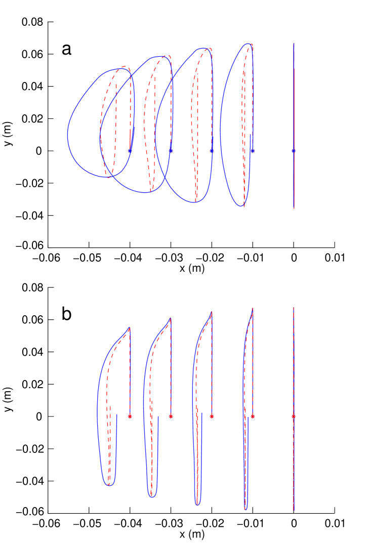
Figure 9: (Color online) Comparison (top view) of the mean trajectories (initially 2 mm above the sphere wall) for 2 mm monodisperse particles starting from the same points for the smooth wall (blue continuous line) and the 2 mm (red dashed lines) rough wall a) in a tumbler filled at 20%; b) in a tumbler filled at 50%.

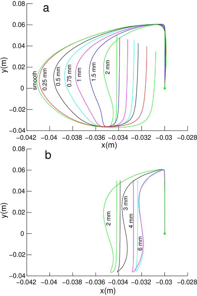
Figure 10: (Color online) Comparison (top view) of the mean trajectories for particles starting from $x=-0.03$ m and 2 mm above the sphere wall for roughnesses ranging a) from a smooth wall to 2 mm rough wall, b) from 2 mm to 6 mm rough walls. The horizontal axis is stretched compared to the vertical axis. The tumbler fill volume is 30%.

Figure 11: Curvature (maximum displacement in one trajectory circulation) of the trajectories and axial drift for tumbler wall roughnesses ranging from smooth (0 mm) to 6 mm rough walls for trajectories starting at $x=-0.03$ m in a 30% full tumbler.

III.3 Dependence on the depth in the flowing layer

To fully understand the nature of the band deformations shown in Figs. 2-5, it is helpful to examine the trajectories at different depths in the flowing layer.

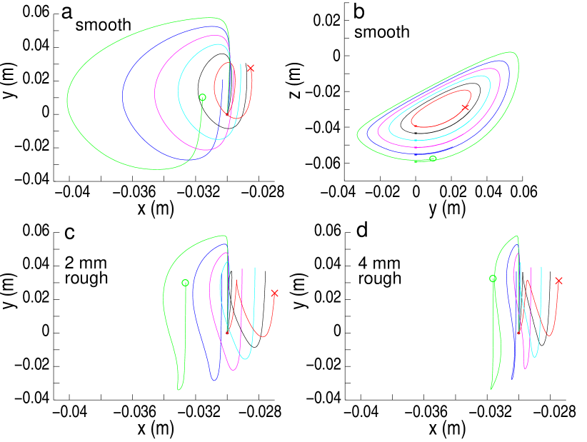
Figure 12: (Color online) Mean trajectories in a spherical tumbler filled at 30% with 2 mm particles flowing at different depth (starting positions 2, 6, 10, 14 and 18 mm above the sphere wall). (a) smooth wall sphere, top view; (b) smooth wall sphere side view; (c) 2 mm rough wall, top view; (d) 4 mm rough wall, top view. The curve ending with a circle is nearest the surface; the curve ending with an X is deepest in the flowing layer.

Figure 12 shows the mean trajectories of particles starting from different vertical positions in the static bed for smooth and two different rough walls. In all cases, trajectories nearer the surface (e.g. green curve ending with a circle) drift toward the pole, while the deepest trajectories (red curve ending with an X) drift toward the equator. For context, the trajectories viewed along the axis of rotation are shown in Fig. 12(b) for smooth walls. The drift toward the poles near the surface and toward the equator deep in the flowing layer in Fig. 2 is consistent with previous studies ZamanDOrtona13 and explains the band deformation evident in Figs. 2-5. The maximum of drift difference (between the surface and the deepest trajectories) occurs for the 2 mm rough wall (Fig. 12(c)) and is slightly less for the 4 mm rough wall (Fig. 12(d)). Indeed the largest deformation of the band is obtained for wall roughnesses of 2 mm and greater (Fig. 4).

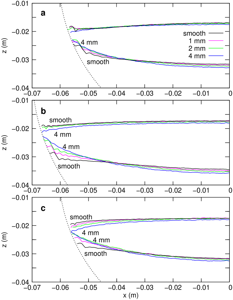
Figure 13: (Color online) Topographies of the surface (top curves) and $v_{y}=0$ lower boundary (bottom curves) of the flowing layer measured for three planes (a) $y=0.035$ m (top of the flow), (b) $y=0$ (middle of the flow), and (c) $y=-0.035$ m (bottom of the flow). The tumbler is filled at 30% with 2 mm particles for smooth, 1 mm, 2 mm, and 4 mm rough walls. The dotted curves show the position of the sphere wall.

Insight into the mechanism for the curved trajectories comes from close examination of the flowing layer. Figure 13 shows the upper free surface and the lower boundary with the fixed bed of particles for the flowing layer at three vertical planes in the flow: upstream ($y=0.035$ m), middle corresponding to the axis of rotation ($y=0$), and downstream ($y=-0.035$ m). The upper surface is based on the upper 0.3 iso-compacity contour, while the lower surface is the position where the out-of-plane velocity is zero: $v_{y}=0$. The jagged appearance for some curves is a consequence of layers of particles adjacent to the walls. For the middle and downstream planes both the free surface and the boundary with the fixed bed become more curved near the wall (dotted curve) as the roughness of the wall increases. Consequently, for larger roughnesses, the flowing layer thickness is reduced near the wall, while for the smooth cases it is thicker indicating that particles may be interacting with the wall differently. In the upper part of the flow, $y=0.035$ m, the flowing layer at the wall has nearly the same thickness regardless of the wall roughness. This behaviour is consistent with the trajectories of the particles in the flow. In the upstream portion of the flowing layer, particles fall away from the wall, so the wall roughness has little impact. In the downstream half of the flowing layer, particles move toward the curved wall and are thus sensitive to its roughness. In the middle portion, particles flow parallel to the wall, and the behavior is intermediate between the upstream and downstream situations.

The dependence of the flowing layer thickness on the wall roughness provides insight into the trajectories of particles. Particles can easily move along a smooth wall, allowing a larger displacement of the trajectories toward the pole. However, the flow is forced away from a rough wall toward the central zone of the tumbler, inducing trajectories with a smaller displacement toward the pole. For even larger roughness, the flow at the wall is so small that the free surface in Fig. 13 curves downward, further reducing displacement toward the poles. The impact of roughness is greatest in the downstream portion of the flowing layer as particles directly impact the wall, inducing a modification to trajectories in which the curvature reverses (Fig. 10(b)). In this way, the flow structure across the entire width of the flowing layer is modified by the roughness of the wall at its periphery.

Similar results occur for fill levels of 50% and 20% at the downstream plane of the flow, but with slight differences. For the 20% case (Fig. 14(a)) the free surface and boundary with the fixed bed are even more important than in the 30% case. Like in the 30% case, the flowing layer thickness at the wall is greatly reduced, especially for larger wall roughness. For the 50% case (Fig. 14(b)), the flowing layer thickness very near the wall is nearly independent of wall roughness. Thus, wall roughness has a much smaller effect on particle trajectories for a 50% fill level (see Fig. 9(b)) than for lower fill levels.

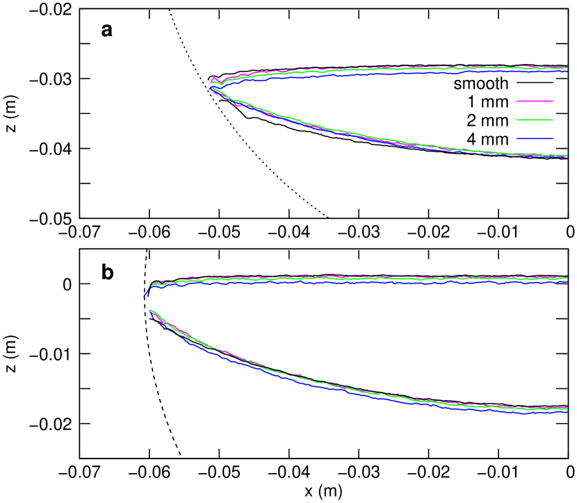
Figure 14: (Color online) Topographies of the surface (top curves) and $v_{y}=0$ boundary (bottom curves) of the granular flow measured in the plane $y=-0.035~{}m$ (bottom of the flow). The tumbler is filled at (a) 20% or (b) 50% with 2 mm particles for smooth, 1 mm, 2 mm, and 4 mm rough walls. The dotted curve shows the position of the sphere wall.

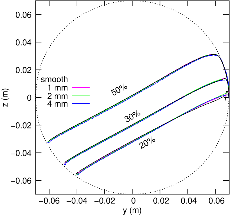
Figure 15: (Color online) Profile of the free surface at the equator for monodisperse 2 mm particles rotated at 15 rpm at $x=0$ for smooth, 1, 2, and 4 mm rough walls. Fill levels are 50% (top curves), 30%, and 20% (bottom curves). For each fill level, the four curves nearly overlay one another.

For completeness, we note that the roughness has no effect on the angle of repose. Figure 15 shows the surface profile at the equator ($x=0$) for various fill levels and wall roughnesses. For each fill level, the free surface profiles for different values of wall roughness nearly overlay each other. A small difference is evident in the upper portion of the 20% fill case. In fact, at that location, the wall is approximately vertical, allowing a monolayer of particles to form in contact with the wall. This monolayer, which has been noted previously at low fill levels in spherical tumblers ChenLueptow09 , reduces the height of the bed of particles just below it. It only occurs for the smooth wall and the 1 mm rough wall.

III.4 Surface velocity, slip at the wall

Based on the dependence of the flowing layer thickness at the wall on wall roughness, it seems that the slip at the wall plays a major role in modifying particle trajectories, changing the velocity profiles, and locally altering the thickness of the flowing layer. To better quantify the slip, we have determined the velocity near the wall along a radial coordinate $x_{w}$ extending normal from the wall at 3 different radial lines a, b, and c (Fig. 16). The velocities $v_{f}$ are measured in the plane parallel to the free surface, but 2 mm below it.

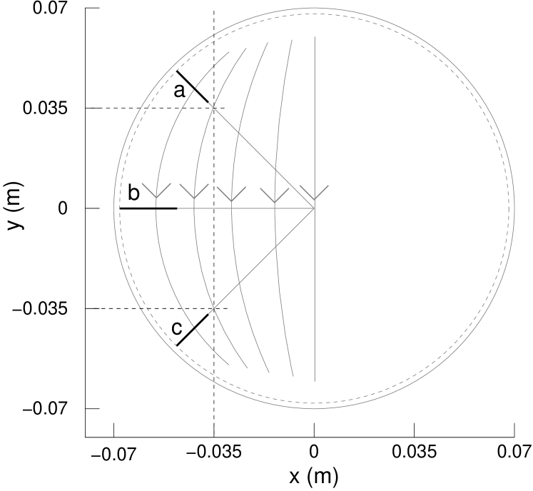
Figure 16: Diagram showing radial lines along which the velocity profiles are measured.

Only the projection of the velocity perpendicular to the radial coordinate and in the plane is considered. The velocities plotted in Fig. 17 are obtained using an interpolation (cubic spline) from the velocity field measured from the simulation. As this velocity field is measured on a cubic grid, only cubes that are completely inside the sphere are used. Hence the velocity profiles do not extend all the way to the wall.

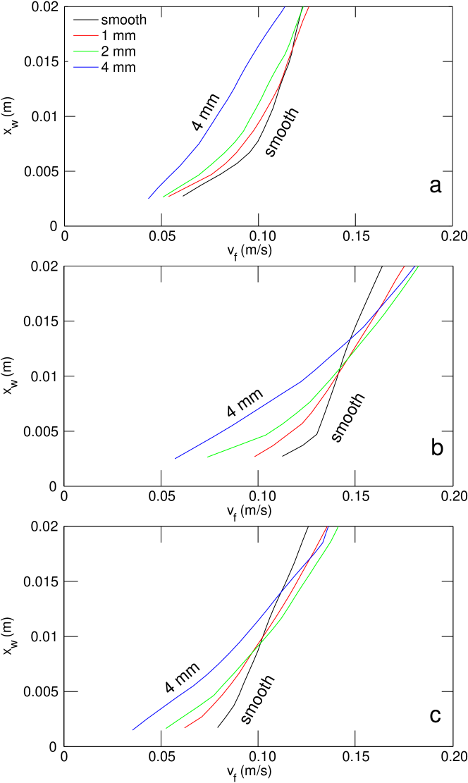
Figure 17: (Color online) Velocity profiles for different wall roughnesses for a 30% filled spherical tumbler at lines a, b, and c in the flowing layer.

In the upper part of the flowing layer at line a (Fig. 17(a)), the velocity very near the wall is similar for all roughnesses, though it appears that slip at the wall is most likely for the smooth wall. This is probably because the particles are moving away from the wall and thus less sensitive to wall roughness. Figure 17(b) shows the velocity profile at line b (mid-length of the flowing layer) where the flow is essentially parallel to the wall. Here the velocity near the wall depends more strongly on the wall roughness with less roughness corresponding to greater likelihood of slip at the wall. Figure 17(c) shows the velocity profile measured close to the wall at line c. Again, wall roughness has significant impact on the velocity near the wall with any tendency for slip decreasing with roughness. Similar results occur for other fill levels, though the 20% fill level is slightly more sensitive to roughness and the 50% fill level is slightly less sensitive to roughness in the downstream portion of the flowing layer.

Figure 18: Slip velocity based on extrapolating the velocity profiles and by measuring the velocity of particles near the wall at line c as a function of wall roughness for 30% fill.

To quantify more precisely the influence of wall roughness on slip, we have estimated the slip velocity at the wall $v_{s}$ in the downstream portion of the flowing layer at c using two different methods. First, the velocity profiles in Fig. 17 were extrapolated with a line to the wall. Second, the velocities of particles within a distance of 1.5 particle radii from the wall and close to the free surface were directly measured. Regardless of the method used to estimate the slip velocity, Fig. 18 shows that the slip at the wall decreases with roughness reaching a limit value at around 3 mm wall roughness, above which increasing roughness does not further affect the wall slip. Note that this value is similar to the roughness in Fig. 11 where the displacement and drift become similar. This result is likely analogous to the situation of an incline in which the maximum friction inducing a minimum flow velocity occurs when the roughness of the incline is approximatively twice the size of the flowing beads GoujonThomas03 .

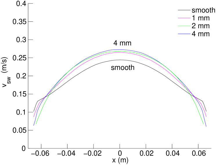
Figure 19: (Color online) Streamwise velocity profiles measured 2 mm below the free surface at the $y=0$ plane for 4 different roughnesses in a 30% filled spherical tumbler.

The impact of the wall boundary condition on the overall flow is also evident in the streamwise velocity (normal to the axis of rotation and in the flowing layer surface) profile at the mid-length of the flowing layer measured 2 mm below the surface (Fig. 19). In the smooth wall case, the velocity near the wall is higher due to slip. As a result, the velocity is lower at the equator. Similar results occur deeper in the flowing layer, as well. It is this difference in the streamwise velocity profiles, combined with the higher flux of particles at the equator as the flowing layer thins for rough walls near its boundary (Figs. 13 and 14) that causes the longer recirculation times in the smooth case than in the rough case, noted with respect to Fig. 2.

III.5 Tumbler rotational speed and size ratio

Finally, we vary both the rotational speed of the tumbler $\omega$ and the ratio of tumbler diameter to particle size ($D/d$) and find that drift and displacement of the trajectories occur even when these key parameters are varied. Consider first results for variations of the rotational speed, shown in Fig. 20,

Figure 20: Displacement and drift for trajectories starting at $x=-0.03$ m, $y=0$ and 2 mm above the bottom wall, for a spherical tumbler filled at 30% with 2 mm particles at various rotation speeds. The walls are perfectly smooth or 2 mm rough.

for 2 mm particles with smooth and 2 mm rough tumbler walls. The displacements for both smooth and rough tumbler walls increase with rotational speed, though the displacements for smooth walls are about twice that for rough tumbler walls. The drift varies little with rotational speed for rough tumbler walls, but decreases slightly with increasing rotational speed for smooth tumbler walls so that it becomes slightly negative by 30 rpm. The difference between smooth walls and rough walls increases with rotation speed for both the drift and the displacement.

Perhaps more interesting is the effect of the tumbler diameter to particle size radio ($D/d$), given that wall roughness affects the flow surprisingly far from the wall for 2 mm particles in a 14 cm tumbler ($D/d=70$). To examine this, we plot particle trajectories for particles that are double and half the particle size used elsewhere in this paper ($d=4$ mm and $d=1$ mm) in Fig 21.

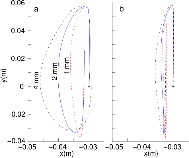
Figure 21: (Color online) Mean trajectories (initially 4 mm above the sphere wall) in a spherical tumbler filled at 30% with particles 1 mm (red dashed), 2 mm (blue solid) and 4 mm (black dashed). The walls are (a) perfectly smooth or (b) rough made of particles of the same size as the flowing particles.

For both smooth and rough walls, large particles have larger displacement than small particles, but the drift only weakly depends on particle size, except for the largest particles. Clearly, the wall roughness significantly affects the flow in all cases, though the impact decreases as the particle size relative to the tumbler size decreases.

Figure 22: Differences (smooth case minus rough case) for drift and displacement versus the size of the particles for trajectories starting at $x=-0.03$ m, $y=0$, and 4 mm above the sphere wall for a tumbler filled at 30%.

Figure 22 shows the difference between smooth and rough wall cases for the displacement and the drift for particle sizes ranging from 1 mm to 4 mm in a 14 cm tumbler. Both displacement and drift differences tend to zero with decreasing particle size, but the decrease is nearly linear. This suggests a remarkable persistence while approaching zero, suggesting that the impact of wall roughness on flow far from the wall persists even to fairly large values of $D/d$. Unfortunately, it is quite difficult to confirm this, since simulations for particles smaller than 1 mm require a very large number of particles and very long computation times.

IV Conclusions

The impact of wall roughness on details of the flow, even far from the bounding wall, can be significant. In a spherical tumbler, wall roughness combined with a curvature of the wall determine the degree of slip at the wall, which in turn affects the flowing layer thickness near the wall. With rough walls and wall orientation such that particles impinge on the wall (the downstream portion of the flowing layer in the spherical tumbler), the resulting decrease in the flowing layer thickness near the wall forces the downstream flux of particles away from the wall. This alters the particle trajectories and the flow even at the equator of the tumbler. On the other hand, smooth walls and wall orientation where particles fall away from the wall result in a higher slip velocity at the wall and consequently, less impact on the flowing layer thickness near the wall. This allows a higher flux of particles near the wall.

The implications for DEM simulations are significant. Even in situations where the walls contact only the periphery of the flow, such as the case of a spherical tumbler, the choice of wall roughness is critical. Preliminary results suggest a similar situation for cylindrical tumblers. Of course, the wall roughness also affects other granular flows, such as straight chute flows, but in these cases the lower wall directly contacts the bottom of the flowing layer, so its impact is not surprising. The global impact of the peripheral flow boundaries may also play a role in situations in which segregation occurs. For instance, bidisperse segregation in spherical tumblers ChenLueptow09 ; NajiStannarius09 and even band formation in bidisperse flows in cylindrical tumblers, where the initial band formation seems to be driven by friction at the cylinder endwalls ChenLueptow11 ; ChenLueptow10 , may be strongly affected by the wall roughness far from the bounding walls. We are investigating these issues further.

References

- (1) J. Schäfer, S. Dippel, and D. E. Wolf, J. Phys. I (France) 6, 5 (1996).
- (2) G. H. Ristow, Pattern Formation in Granular Materials (Springer-Verlag, Berlin, 2000).
- (3) P. A. Cundall and O. D. L. Strack, Géotechnique 29, 47 (1979).
- (4) S. Shoichi, Mod. Phys. Lett. B 12, 115 (1998).
- (5) D. Hirshfeld and D. C. Rapaport, Eur. Phys. J. E 4, 193 (2001).
- (6) G. H. Ristow, Europhys. Lett. 28, 97 (1994).
- (7) J. J. McCarthy and J. M. Ottino, Powder Technol. 97, 91 (1998).
- (8) M. Moakher, T. Shinbrot, and F. J. Muzzio, Powder Technol. 109, 58 (2000).
- (9) R. Y. Yang, R. P. Zou, and A. B. Yu, Powder Tech. 130, 138 (2003).
- (10) K. Yamane, M. Nakagawa, S. A. Altobelli, T. Tanaka, and Y. Tsuji, Phys. Fluids 10, 1419 (1998).
- (11) P. Chen, J. M. Ottino, and R. M. Lueptow, New J. Phys. 13, 055021 (2011).
- (12) N. Taberlet, W. Losert, and P. Richard, Europhys. Lett. 68, 522 (2004).
- (13) D. C. Rapaport, Phys. Rev. E 65, 061306 (2002).
- (14) N. Taberlet, M. Newey, P. Richard, and W. Losert, J. Stat. Mech. P07013 (2006).
- (15) F. da Cruz, S. Emam, M. Prochnow, J.-N. Roux, and F. Chevoir, Phys. Rev. E 72, 021309 (2005).
- (16) T. Pöschel and V. Buchholtz, Chaos, Solitons and Fract., 5, 1901 (1995).
- (17) G. Juarez, P. Chen, and R. M. Lueptow New J. Phys. 13, 053055 (2011).
- (18) F. Bertrand, L. A. Leclaire, and G. Levecque, Chem. Eng. Sci. 60, 2517 (2005).
- (19) F. Pignatel, C. Asselin, L. Krieger, I. C. Christov, J. M. Ottino, and R. M. Lueptow, Phys. Rev. E 86, 011304 (2012).
- (20) N. Taberlet, P. Richard, A. Valance, W. Losert, J. M. Pasini, J. T. Jenkins, and R. Delannay, Phys. Rev. Lett. 91, 264301 (2003).
- (21) S. W. Meier, R. M. Lueptow, and J. M. Ottino, Adv. Phys. 56, 757 (2007).
- (22) S. Courrech du Pont, P. Gondret, B. Perrin, and M. Rabaud, Europhys. Lett. 61, 492 (2003).
- (23) Z. Zaman, U. D’Ortona, P. B. Umbanhowar, J. M. Ottino, and R. M. Lueptow, Phys. Rev. E 88, 012208 (2013).
- (24) C. Goujon, N. Thomas, and B. Dalloz-Dubrujeaud, Eur. Phys. J. E 11, 147 (2003).
- (25) D. A. Augenstein, Powder Tech. 19, 205 (1978).
- (26) A. R. Thornton, T. Weinhart, S. Luding, and O. Bokhove, Eur. Phys. J. E 35, 127 (2012).
- (27) T. Weinhart, A. R. Thornton, S. Luding, and O. Bokhove, Gran. Matter 14, 531 (2012).
- (28) C. Ancey, Phys. Rev. E 65, 011304 (2001).
- (29) C. S. Campbell, J. Fluid Mech. 247, 111 (1993).
- (30) C. S. Campbell, J. Fluid Mech. 247, 137 (1993).
- (31) F. Verbücheln, E. J. R. Parteli, and T. Pöschel, Soft Matter 11, 4295 (2015).
- (32) P. Chen, J. M. Ottino, and R. M. Lueptow, Phys. Rev. E 78, 021303 (2008).
- (33) M. P. Allen and D. J. Tildesley, Computer Simulation of Liquids (Oxford University Press, New York, 2002).
- (34) T. G. Drake and R. L. Shreve, J. Rheol. 30, 981 (1986).
- (35) S. F. Foerster, M. Y. Louge, H. Chang, and K. Allia, Phys. Fluids 6, 1108 (1994).
- (36) C. S. Campbell, J. Fluid Mech. 465, 261 (2002).
- (37) L. E. Silbert, G. S. Grest, R. Brewster, and A. J. Levine, Phys. Rev. Lett. 99, 068002 (2007).
- (38) P. Chen, J. M. Ottino, and R. M. Lueptow, Phys. Rev. Lett. 104, 188002 (2010).
- (39) P. Chen, B. J. Lochman, J. M. Ottino, and R. M. Lueptow, Phys. Rev. Lett. 102, 148001 (2009).
- (40) L. Naji and R. Stannarius, Phys. Rev. E 79, 031307 (2009).