Evolution, nucleosynthesis and yields of AGB stars at different metallicities (III): intermediate mass models, revised low mass models and the ph-FRUITY interface.

Abstract

We present a new set of models for intermediate mass AGB stars (4.0, 5.0 and, 6.0 M_⊙) at different metallicities (-2.15$\leq$[Fe/H]$\leq$+0.15). This integrates the existing set of models for low mass AGB stars (1.3$\leq$M/M_⊙$\leq$3.0) already included in the FRUITY database. We describe the physical and chemical evolution of the computed models from the Main Sequence up to the end of the AGB phase. Due to less efficient third dredge up episodes, models with large core masses show modest surface enhancements. The latter is due to the fact that the interpulse phases are short and, then, Thermal Pulses are weak. Moreover, the high temperature at the base of the convective envelope prevents it to deeply penetrate the radiative underlying layers. Depending on the initial stellar mass, the heavy elements nucleosynthesis is dominated by different neutron sources. In particular, the s-process distributions of the more massive models are dominated by the ²²Ne($\alpha$,n)²⁵Mg  reaction, which is efficiently activated during Thermal Pulses. At low metallicities, our models undergo hot bottom burning and hot third dredge up. We compare our theoretical final core masses to available white dwarf observations. Moreover, we quantify the weight that intermediate mass models have on the carbon stars luminosity function. Finally, we present the upgrade of the FRUITY web interface, now also including the physical quantities of the TP-AGB phase of all the models included in the database (ph-FRUITY).

1 Introduction

Asymptotic Giant Branch (AGB) stars are ideal laboratories to test our understanding of stellar interiors. The evolution of those objects is characterized by a sequence of burning and mixing episodes, which carry the nuclear products synthesized in the internal layers to the stellar surface. During the AGB, the structure consists of a partially degenerate CO core, a He-shell and a H-shell separated by a thin helium rich layer (the so-called He-intershell) and, an expanded and cool convective envelope. The surface luminosity is mainly sustained by the H-burning shell. This situation is recurrently interrupted by the growing up of thermonuclear runaways (Thermal Pulse, TP) in the He-intershell, triggered by the activation of 3$\alpha$ reactions. The rate of nuclear energy is too large to be carried away by radiation and, thus, a convective shell develops, which makes the He-intershell chemically homogenous. Then, the layers above expand and cool until the convective shell quenches. If the expansion has been large enough, the H-shell switches off and the convective envelope can penetrate the H-exhausted and chemically enriched He-intershell (this phenomenon is known as the Third Dredge Up, TDU). Meanwhile, the products of internal nucleosynthesis appear on the stellar surface. During the AGB, a strong stellar wind erodes the convective envelope, thus polluting the interstellar medium. AGB stars efficiently synthesize light (C, N, F and Na) as well as heavy elements (those created via the slow neutron capture process, the s-process). The interested reader can find a vast literature on AGB stars (Iben & Renzini, 1983; Herwig, 2005; Straniero et al., 2006; Karakas & Lattanzio, 2014).
In order to properly describe the chemical evolution of the hosting systems, sets of AGB yields as much uniform and complete as possible are needed. In the past years, we made our AGB yields available on the FRUITY database (Cristallo et al., 2009, 2011). Through a web interface, we provide tables of isotopic and elemental compositions as well as stellar yields of AGB stars. Up to date, FRUITY includes low mass stars only (i.e. stars with initial masses M$\leq$ 3 M_⊙). In this paper, we present a new set of AGB models with larger initial masses (4$\leq$ M/M_⊙$\leq$6). The evolution of those objects resembles that of their low mass counterparts, even if noticeable differences exist. In particular, their larger initial masses produce more compact cores and, thus, larger temperatures can be attained in their interiors. As a consequence, the physical conditions to trigger the He-burning in the He-intershell are attained earlier during the AGB phase with respect to models with lower initial masses. Thus, the interpulse phases are shorter, the TPs are weaker and the efficiency of TDU is strongly reduced (Straniero et al., 2003a). Moreover, the larger the initial stellar mass, the larger the mass extension of the convective envelope (this fact implying a larger dilution of the dredged up material). As a consequence, we obtain modest surface chemical enrichments in the more massive AGBs. Furthermore, in those objects processes like the Hot Bottom Burning (HBB; Sugimoto 1971; Iben 1973) and the Hot-TDU (H-TDU; Goriely & Siess 2004; Straniero et al. 2014) can be active. During the HBB, temperature becomes high enough to partially activate the CN cycle at the base of the convective envelope. As a consequence, considerable amounts of ¹³C and ¹⁴N can be produced. The main effect of H-TDU, instead, is to limit the penetration of the convective envelope itself, because the temperature for the reactivation of the H-shell is attained soon. Thus, H-TDU further weakens the TDU efficiency.
In AGB stars, two major neutron sources are at work: the ¹³C($\alpha$,n)¹⁶O and the ²²Ne($\alpha$,n)²⁵Mg reactions. In low mass stars, the dominant contribution to s-process nucleosynthesis comes from the ¹³C($\alpha$,n)¹⁶O reaction. The ¹³C reservoir, the so-called ¹³C pocket, forms during TDU episodes in the top layers of the H-exhausted He-intershell (for details see Cristallo et al. 2011). In more massive AGBs, due to the limitations of the H-TDU, the contribution from the ¹³C reaction is definitely lower, while an important contribution comes from the ²²Ne($\alpha$,n)²⁵Mg . In fact, in those objects this reaction is efficiently activated at the base of the convective shells generated by TPs. This neutron source significantly contributes to the production of rubidium and light s-process elements. Thus, s-process surface distributions with different shapes and enhancements can be found by varying the metallicity and the initial stellar mass. In fact, the three s-process peaks receive different contributions depending on the physical environmental conditions (radiative or convective burning) and on the neutron-to-seed ratio (which is related to the metallicity).
In this paper we also illustrate a new web interface (ph-FRUITY), to access tables containing the evolution of the most relevant physical quantities of our models.
This paper is structured as follows. In §2 we describe the main features of our stellar evolutionary code, focusing on the most recent upgrades. In §3 we highlight the evolutionary phases prior to the AGB, which is analyzed in §4. In §5 we show the potentiality of our new web ph-FRUITY interface. The nucleosynthesis of all FRUITY models is discussed in detail in §6. Finally, in §7 we report the discussion and our conclusions.

2 The models

As already outlined, models presented in this paper (4.0-5.0-6.0 M_⊙) integrate the already existing set available on the FRUITY database (Cristallo et al., 2011), currently hosting Low Mass Stars AGB models (hereafter LMS-AGB; 1.3-1.5-2.0-2.5-3.0) with different initial metallicities (-2.15$\leq$[Fe/H]$\leq$+0.15). We add a further metallicity ($Z=0.002$, corresponding to [Fe/H]=-0.85) in order to better sample the peak in the lead production (see below). In Table 1 we report all the models included in the FRUITY database (in bold the models added with this work), by specifying the initial He content, the [Fe/H] and the eventual $\alpha$ enrichment. In the Table header we report both the [Fe/H] and the corresponding total metallicity (which takes into account for the eventual $\alpha$ enhancement). The isotopic initial distribution of each model is assumed to be solar-scaled (apart from eventual $\alpha$-enhanced isotopes, i.e. ¹⁶O, ²⁰Ne, ²⁴Mg, ²⁸Si, ³²S, ³⁶Ar and, ⁴⁰Ca). We adopt the solar distribution presented by Lodders (2003). The models have been computed with the FUNS evolutionary code (Straniero et al., 2006; Cristallo et al., 2009). The physical evolution of the star is coupled to a nuclear network including all isotopes (from hydrogen to lead, at the termination of the s-process path). Thus, we do not need to perform any post-process calculation to determine the nucleosynthetic yields. The list of reactions and the adopted rates are the same as in Cristallo et al. (2011). Among the various physical processes, convection and mass-loss mainly affect the AGB evolution (and, thus, the correlated stellar yields and surface distributions). We determine convective velocities following the prescriptions of the Mixing Length Theory (MLT; Böhm-Vitense 1958), according to the derivation of Cox (1968). In the framework of the MLT, in correspondence to a convective border the velocity is zero, if the adiabatic temperature gradient presents a smooth profile. However, during a TDU episode there is a sharp discontinuity in the opacity profile (and, thus, in the radiative gradient). This makes the convective/radiative interface unstable. In order to handle such a situation, we apply an exponentially decreasing profile of convective velocities below the formal Schwarzschild border (Straniero et al., 2006). This implies a more efficient TDU and, as a by-product, the formation of a tiny ¹³C pocket. In fact, such a non-convective mixing allows some protons to penetrate the formal border of the convective envelope. Those protons are captured by the abundant ¹²C (the product of 3$\alpha$ processes) leading to the formation of a region enriched in ¹³C (commonly known as the ¹³C-pocket). In Cristallo et al. (2009) we demonstrated that the extension in mass of the ¹³C pocket decreases along the AGB (thus with increasing core masses), following the shrinking and the compression of the He-intershell region. Therefore, we expect that the contribution to the s-process nucleosynthesis from the ¹³C pocket is strongly reduced in massive AGBs with respect to their low-mass counterparts (see §4). In the following, we define Intermediate Mass Stars (IMS) those approaching the TP-AGB phase with a mass of the H-exhausted core greater than 0.8 M_⊙ (see §3).
Another very uncertain physical input for AGB models is the mass-loss rate, which largely determine, for instance, the duration of the AGB and the amount of H-depleted dredged-up material after each TDU. During the AGB, large amplitude pulsations induce the formation of shocks in the most external stellar layers. As a result, the local temperature and density increase and a rich and complex chemistry develops, leading to the creation of molecules and dust grains. Those small particles interact with the radiation flux and drive strong stellar winds. Available observational data indicate that in galactic AGB stars the mass loss ranges between $10^{-8}$ and $10^{-4}$ $M_{\odot}$/yr, with a clear correlation with the pulsational period (Vassiliadis & Wood, 1993), at least for long periods (see Uttenthaler 2013). Since the latter depends on the variations of radius, luminosity and mass, a relation between the mass loss rate and the basic stellar parameters can be derived. By adopting a procedure similar to Vassiliadis & Wood (1993), we revised the mass loss-period relation, taking in to account more recent infrared observations of AGB stars (see Straniero et al. 2006 and references therein) and basing on the observed correlation between periods and luminosities in the K band (see e.g. Whitelock et al. 2003). The few pulsational masses derived to date for AGB stars (Wood, 2007) do not allow the identification of trends in the mass loss-period relation as a function of the stellar mass. Thus, we apply the same theoretical recipe for the whole mass range in our models, even if other mass-loss prescriptions are available for luminous oxygen rich AGB giants. For instance, we could use the mass-loss rate proposed by van Loon et al. (2005). However, when applying that formula to our low metallicity models, the mass loss practically vanishes and, therefore, we exclude it.
When dealing with C-rich objects, particular attention must be paid to the opacity treatment of the most external (and cool) regions. As already discussed, molecules efficiently form in those layers. Depending on the C/O ratio, O-bearing or C-bearing molecules form, leading to dichotomic behaviors in the opacity regime. C-bearing molecules, in fact, are more opaque and, thus, increase the opacity of the layer where they form. As a consequence, the radiation struggles to escape from the stellar structure and, as a consequence, the most external layers expand and cool. This naturally implies an enhancement in the mass-loss rate, which strongly depends on the stellar surface temperature. We demonstrated that the use of low temperature C-bearing opacities has dramatic consequences of the physical evolution of AGB stars (Cristallo et al. 2007; see also Marigo 2002 and Ventura & Marigo 2010). For solar-scaled metallicities, we adopt opacities from Lederer & Aringer (2009), while for $\alpha$ enhanced mixtures we use the AESOPUS tool (Marigo & Aringer, 2009), which allows to freely vary the chemical composition. In calculating the IMS-AGB models, we found an erroneous treatment of opacities in the most external layers of the stars, enclosing about 2% of the total mass. Then, we verified one by one all the low mass models already included in the FRUITY database and for some of them we found significative variations in the final surface composition. We discuss this problem in §6.

3 From the pre-main sequence to the thermal pulse AGB phase

We follow the evolution of the models listed in Table 1 from the pre-Main Sequence up to the AGB tip. The computations terminate when the H-rich envelope is reduced below the threshold for the TDU occurrence. The Hertzsprung-Russell tracks of the solar metallicity set are shown in Figure 1.
In this Section we briefly revise the evolution until the beginning of the TP-AGB phase. For a more detailed description of these phases see Dominguez et al. (1999). All the evolutionary sequences start from a homogeneous and relatively cool model relaxed on the Hayashi track, i.e., the first fully convective models in hydrostatic and thermal equilibrium. As usual, stars enter the Main Sequence (MS) when all the secondary isotopes involved in the p-p chain and the CNO cycle attain the equilibrium in the central region. Table 2 report MS lifetimes for the whole data set. In Equation 1, we provide a simple interpolation formula linking the MS lifetime to the initial mass and metallicity of the model:

$$\tau_{\rm MS}=9.775+9.898*Z-1.460*ln(M)+0.152*(ln(M))^{2}$$ (1)

The variations of these lifetimes reflect the well-known non-linearity of the mass-luminosity relation for MS stars. The less massive models (1.3 M_⊙) mark the transition between the lower MS (consisting of stars whose luminosity is mainly controlled by the p-p nuclear chain and characterized by a radiative core and a convective envelope) and the upper MS (whose stars burn H through the CNO cycle and develop a convective core, while their envelope remains fully radiative). The convective core attains a maximum extension just after the beginning of the MS. Then, its extension decreases, as H is converted into He and, consequently, the radiative opacity decreases. The maximum extension of the convective core is reported in Table 3. No convective core overshoot has been assumed in these models. Central convection eventually disappears when the central H mass fraction drops below $\sim 0.1$. Then, an overall contraction occurs. The tip of the MS, i.e., the relative maximum in the luminosity, is attained when the central H goes to $\sim 0$. Then, before He ignition, all the models, except the more massive with $Z\leq 10^{-3}$, experience a deep mixing episode, the so-called first dredge up (FDU).

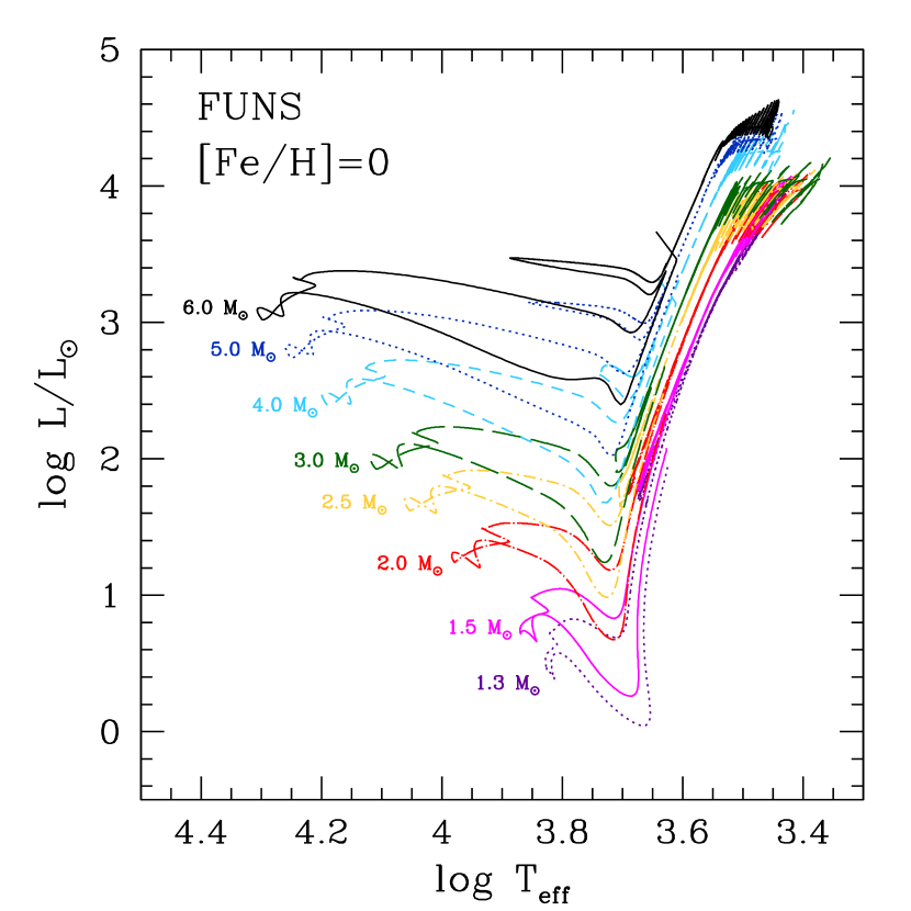
Figure 1: Hertzsprung-Russell diagram for models with initial solar metallicity.

The following development of the He burning depends on the equation of state of the He-rich core. The values of the He-core masses at the ignition well represent this occurrence, as reported in Table 4. For the more massive models (M$\geq 3$ M_⊙), they are essentially determined by the extension of the convective core during the main sequence. After the core-H burning, these stars rapidly proceed toward a quiescent He ignition that occurs at relatively low density. On the contrary, for less massive stars the core mass slowly grows during the RGB, because of the shell H-burning. For this reason, in stars with M$<2$ M_⊙, the central density grows up to $10^{5}$-$10^{6}$ g/cm³ so that the pressure is mainly controlled by degenerate electrons. Under these conditions, the He ignition proceeds through a thermonuclear runaway (He flash), when the core mass exceeds a critical value of about 0.5 M_⊙. In slightly more massive objects ($2<M/M_{\odot}<$3), the electron degeneracy is weaker and the critical core mass for the He ignition is reduced down to $\sim 0.3$ M_⊙ (see Prada Moroni & Straniero 2009). This behavior is also illustrated in Figure 2; the minimum core mass at the He ignition is found for stellar masses $2.0<$M/M${}_{\odot}<2.5$ (see also Sweigart et al. 1990; Dominguez et al. 1999).

Figure 2: He-exhausted core masses at the beginning of central He burning (pentagons), at the end of central He burning (triangles), at the beginning of the AGB (squares) and, at the end of AGB (circles).

Table 5 reports the core He burning lifetimes. The variation of this quantity reflects the variations of the core mass at the He ignition. In fact, the lower the core mass, the fainter the He burning phase and, in turn, the longer the lifetime. As a result, the longest core He burning lifetimes are attained for stellar masses between 2 and 2.5 M_⊙. Our core He burning models include specific treatments of the instability occurring at the external border of the convective core and semi-convection, as described in Straniero et al. (2003b). During this phase, the core mass further increases, due to the work done by the shell H burning (see Figure 2). For high metallicities, at the end of the core He burning phase, the core mass is nearly constant for M$<3$ M_⊙ and rapidly increases for larger stellar masses. This limit is smaller at lower Z. The masses of the H-exhausted core at the end of the central He burning phase are reported in Table 6.
During the early-AGB phase, an He burning shell forms and advances in mass at a rate much higher than that of the pre-existing H burning shell. In the more massive models, the H burning dies down and another mixing episode occurs (the Second Dredge Up, SDU), owing to the expansion powered by the He burning and the consequent cooling of the envelope. The lowest stellar mass undergoing a SDU is the 3 M_⊙ at $Z$=0.0001 and the 4 M_⊙ at $Z$=0.02. Table 7 lists the core mass at the onset of the first thermal pulse. It practically coincides with the value attained at the end of the core-He burning, except for stars undergoing the SDU, as clearly shown in Figure 2.
Due to the mass lost in the previous evolutionary phases, stars attain the AGB with masses lower than the initial ones. In our models, we adopt a Reimers’ parametrization of the mass-loss rate (with $\eta=0.4$) up to the first TP. In general, only stars with M$\leq 2$ M_⊙ (those developing a degenerate He-rich core during the RGB) lose a non negligible fraction of their initial mass (see Table 8).
The modifications of the chemical compositions induced by the FDU and (eventually) the SDU are reported in Tables 9 and 10 for two different metallicities ($Z=1\times 10^{-2}$ and $Z=2.4\times 10^{-4}$, respectively). As expected, after a dredge up episode (FDU or SDU) the models show an increase in the surface helium abundance as well as modified CNO isotopic ratios. It should be noted that the abundances observed at the surface of low mass (M$<$ 2.0 M_⊙) giant stars at the tip of the RGB often differ from those at FDU due to the presence of a non-convective mixing episode, which links the surface to the hot layers above the H-burning shell. This occurs when stars populate the so-called bump of the luminosity function (see Palmerini et al. 2011 for a discussion on the various proposed physical mechanisms triggering such a mixing; see also Nucci & Busso 2014). Those chemical anomalies have been observed, for instance, in low metallicity stars (Gratton et al., 2000) and measured in oxide grains (Al₂O₃) of group 1 (Nittler et al., 1997). Considering that, up-to-date, no definitive theoretical recipe exists for this non-convective mixing, our models do not include any RGB extra-mixing. Among the isotopes reported in Table 9 and Table 10, the most sensitive isotopes to an extra-mixing process should be ¹³C and ¹⁸O. This has to be kept in mind when adopting our isotopic abundances.

4 The TP-AGB phase (I): physics

FUNS models with mass 1.3$\leq$M/M_⊙$\leq$3.0 has been extensively analyzed in Cristallo et al. (2009) and Cristallo et al. (2011). However, in order to provide a general picture of stellar evolution during the AGB phase, some of their physical properties will be addressed here again.
In order to evaluate the behavior of the TDU mechanism as a function of the mass and the metallicity, we plot the ratio between the mass of H-depleted dredged-up material at each TDU ($\delta M_{TDU}$) and the envelope mass as a function of the mass of the H-exhausted core in Figure 3. Such a quantity provides an estimation of the TDU efficiency in polluting the convective envelope. This Figure shows that at Z=$10^{-2}$ (upper panel) a star with initial mass M=1.3 M_⊙ is close to the lower mass limit to experience TDU. The maximum TDU efficiency is reached for the 3 M_⊙ model. Then, there is an abrupt drop in the TDU efficiency in correspondence to the 4 M_⊙ model. In fact, the physical structure of this model is deeply different with respect to those of lower masses. In particular, the mass of the H-exhausted core (M_H) is definitely larger.

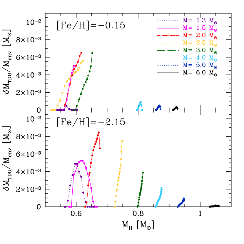
Figure 3: Ratio between the mass of H-depleted dredged-up material ($\delta$M_TDU) and the envelope mass (M_env) for different masses at Z=$10^{-2}$ (upper panel) and Z=$2.4\times 10^{-4}$ (lower panel).

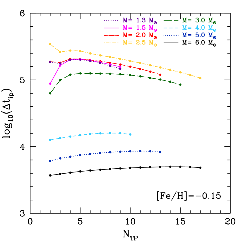
Figure 4: Interpulse duration for models with Z=10^-2.

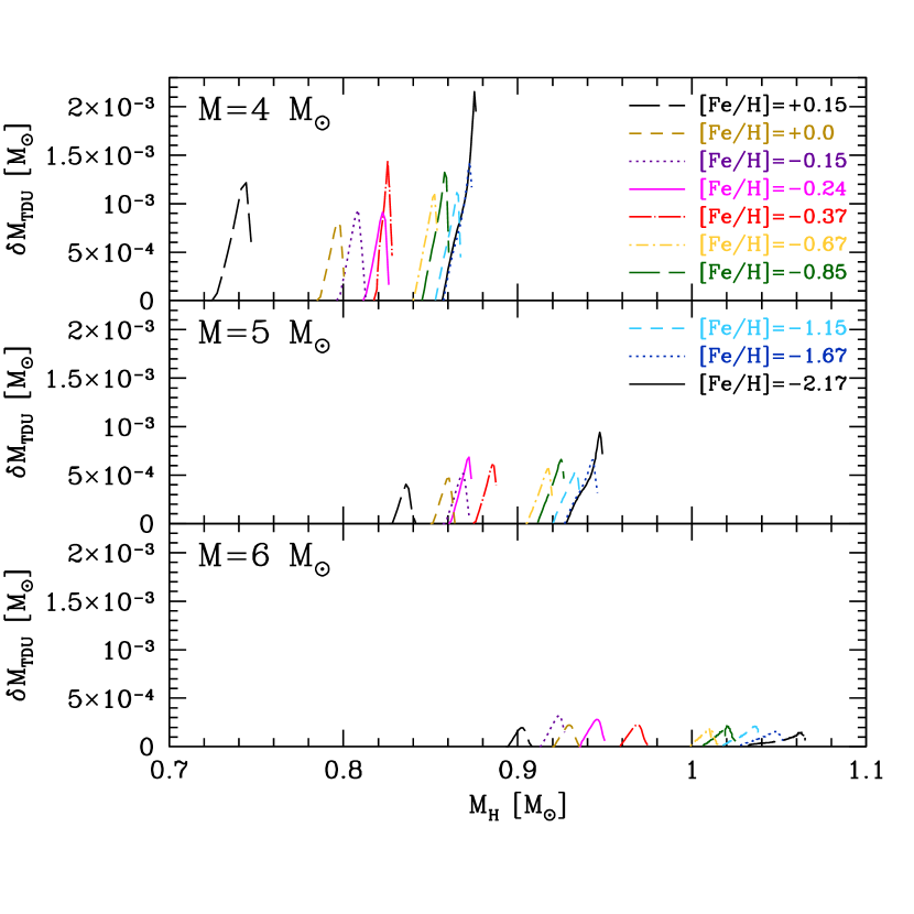
Figure 5: Mass of H-depleted dredged-up material at each TDU for models with initial mass M=4 M_⊙ (upper panel), M=5 M_⊙ (middle panel) and M=6 M_⊙ (lower panel).

This implies a larger compression of the H-exhausted layers and, thus, the He-intershell is thinner and hotter. As a consequence, the time needed to reach the ignition conditions for the 3$\alpha$ process during H-shell burning is shorter. Hence, the interpulse period decreases and, finally, the TDU efficiency is lower (Straniero et al., 2003a). In Figure 4 we report the interpulse phase duration ($\Delta t_{\rm ip}$) for models with Z=$10^{-2}$. While for models with M$\leq$ 3 M_⊙ the $\Delta t_{\rm ip}\geq 10^{5}$, for larger masses it decreases to $10^{4}$ yr and 5000 yr for the 4 M_⊙ and 6 M_⊙, respectively. As shown in the lower panel of Figure 3, at low metallicities even the lowest masses (1.3-1.5 M_⊙) experience a deep TDU, due to the low CNO elemental abundances in the envelope (which implies a reduced H-shell efficiency). Moreover, the transition between LMS-AGBs and IMS-AGBs is smoother, as the 2.5 and 3.0 M_⊙ models start the TP-AGB phase with definitely larger core masses with respect to their high-metallicity counterparts. More massive models (4-5-6 M_⊙) are characterized by a very low TDU efficiency (as their metal-rich counterparts), but show a definitely larger number of TPs (see Table 11). This is due to the fact that the stellar structure is more compact and, thus, the external layers are hotter. As a consequence, the mass-loss erodes the convective envelope at a lower rate and the star experiences a larger number of TPs. In Figure 5 we report the $\delta M_{\rm TDU}$ for all the computed IMS-AGB models. As already highlighted, in the 6 M_⊙ model there is no trend with the initial metallicity, the TDU efficiency being always very low. In the 5 M_⊙ models there is a slight increase of TDU efficiency at low metallicities. For $Z\leq Z_{\odot}$, the 4 M_⊙ models show a clear increase of the TDU efficiency by decreasing the initial iron content. The $Z=2\times 10^{-2}$ model represents an exception, because it shows a net increase of the TDU efficiency. In fact, the core at the beginning of the TP-AGB is less massive than that of models with lower $Z$ and, thus, an increase of the TDU efficiency is expected. In Table 12 we report the cumulative dredged up mass (in M_⊙) for different initial masses and metallicities ($\Delta M_{\rm TDU}$). As expected, models with the largest $\Delta M_{\rm TDU}$ are in the range 2-2.5 M_⊙ and, thus, the major pollution of the interstellar medium is expected from these objects (see §6). Another way to evaluate the TDU efficiency is to analyze the behavior of the $\lambda$ values, defined as the ratios between the mass of H-depleted dredged-up material and the mass growth of the H-exhausted core during the previous interpulse phase (see Figures 6 and 7). At solar-like metallicities, the maximum values of $\lambda$ we obtain is $\sim 0.5$, for stars with M$\geq 2.0$ M_⊙. At low Z, instead, the $\lambda$ grows up to 0.8, implying a larger TDU efficiency.

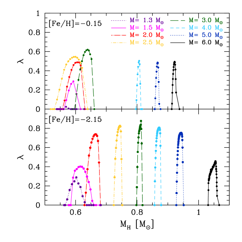
Figure 6: As in Figure 3, but for the $\lambda$ values, defined as the ratios between mass of H-depleted dredged-up material and the growth of the H-exhausted core during the previous interpulse phase.

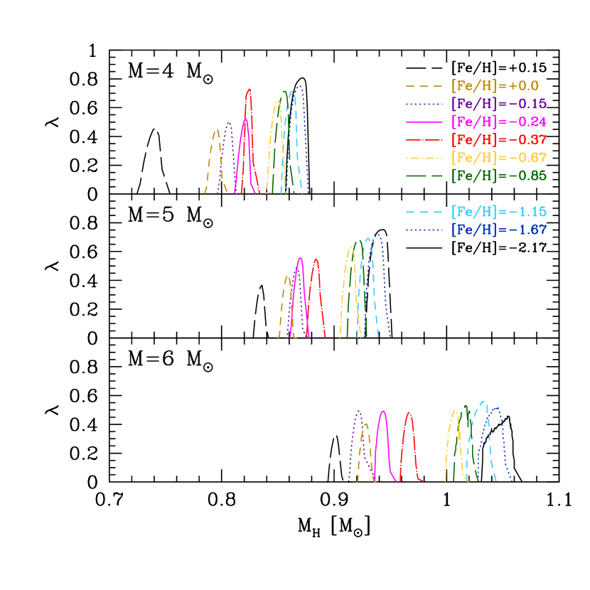
Figure 7: As in Figure 5, but for the $\lambda$ values.

Depending on the final C/O ratio, stars are classified as C-rich objects (C/O$>$1) or O-rich objects (C/O$<$1). The final surface C/O ratio depends on many factors, whose effects are not easy to be disentangled. Among them, the TDU efficiency and the mass-loss rate play a major role. The uncertainties affecting these phenomena have been extensively reviewed in Ventura & D’Antona (2005a, b). They show that very different results can be obtained by modifying, within uncertainties, the recipe adopted to treat them. In §7 we will compare our models to similar computations described in the recent literature.
While the TDU efficiency is strictly connected to the mixing algorithms adopted to compute the models (mixing scheme; treatment of convective borders; etc), the number of TDU mainly depends on the mass-loss mechanism. The latter, in fact, erodes the mass of the convective envelope and determines the dilution factor between the cumulatively dredge up material and the envelope mass itself. Thus, if the envelope mass is not too large and the number of experienced TDUs is high enough, the model shows C/O$>$1 at the surface. Once again, the duration of the C-rich phase depends on the efficiency of mass-loss in eroding the convective envelope. As already stressed, the presence of carbon bearing molecules locally increases the opacity. Thus, we expect an increase of the mass loss rate when the C/O becomes greater than 1.
In Table 13, we report the total TP-AGB lifetimes ($\tau_{\rm TP-AGB}$) for all FRUITY models. Models which are still O-rich at the end of their evolution are labelled as O, while models ending their evolution with a surface C/O$>$1 are labelled as C. Numbers in brackets refer to the percentage of the TP-AGB phase spent in the C-rich regime. As it can be seen, all the models become C-rich at low metallicities and spend the majority of their TP-AGB lifetime in the C-rich regime. This can also be appreciated in Figure 8, where we report $\tau_{\rm TP-AGB}$ (histograms) and the corresponding time spent during the C-rich regime (shaded histograms) for three different metallicities ($Z=2\times 10^{-2}$: upper panel; $Z=6\times 10^{-3}$: middle panel; $Z=1\times 10^{-3}$: lower panel). In general, the larger the metallicity, the longer the TP-AGB lifetimes and the lower the time fraction spent in the C-rich regime. The lifetimes of IMS-AGBs are definitely shorter (about a factor 10) with respect to LMS-AGBs. From Figure 8, it turns out that stars with the longest TP-AGB lifetimes have M=2.5 M_⊙ for large and intermediate metallicities. At low Z, instead, we find a monotonic trend, with the lowest masses showing the longest $\tau_{\rm TP-AGB}$.

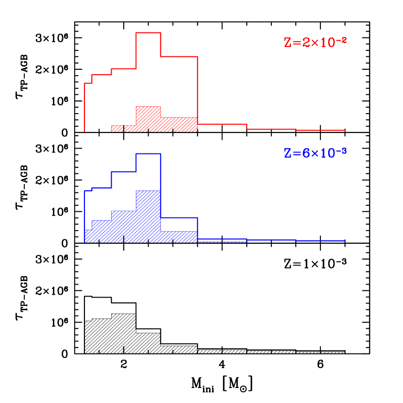
Figure 8: TP-AGB lifetimes for three selected metallicities. Shaded histograms refer to the C-rich phase of the models.

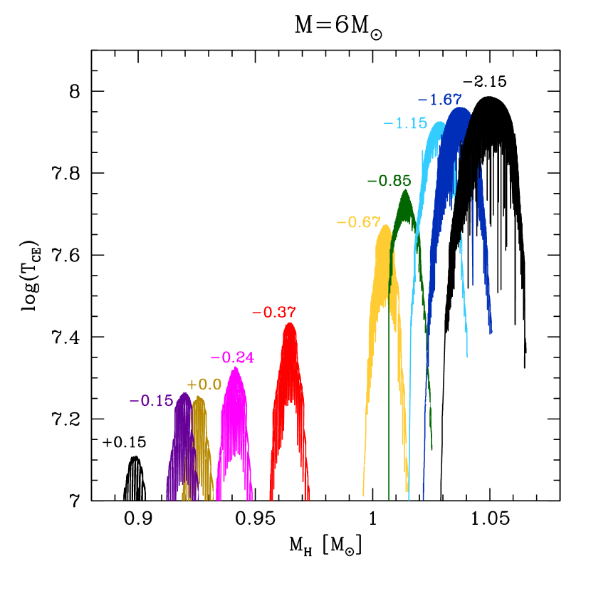
Figure 9: Evolution of the temperature attained at the base of the convective envelope during the TP-AGB phase of 6 M_⊙ models at different [Fe/H].

Note that the HBB and the H-TDU could be at work during the TP-AGB phase. Both phenomena are able to modify the surface C/O ratio. In Figure 9, we report the maximum temperature attained at the base of the convective envelope during the TP-AGB phase of 6 M_⊙ models at different metallicities. In order to efficiently activate the HBB, the base of the convective envelope should attain 80 MK. In our models, this condition is fulfilled at the lowest metallicities for the largest masses (5-6 M_⊙) only. Another interesting phenomenon, possibly working during the TP-AGB phase, is the H-TDU. In this case, the temperature at the base of the convective envelope is high enough to restart the H-burning during a TDU episode. As a result, protons are mixed and burnt on-flight. In our models, H-TDU is activated at low metallicities only, with particular high efficiencies in the more massive models. The effects of HBB and H-TDU on the nucleosynthesis of our models are discussed in §6. Considering that the envelopes of AGB stars are very expanded ($R\sim 200-1000$ R_⊙) and that the average convective velocity is low ($v\sim 10^{5}$ cm s^-1), for some isotopes the convective turnover timescale is longer than the proton capture timescales at the base of the convective envelope. In order to properly treat those processes, the computation of the chemical evolution should be performed by coupling mixing and burning. We intend to address it in a future study. Models presented in this paper have been calculated with a 3 step process. First, we burn chemicals over a model time step. Then, we mix them in convective regions following a time-dependent mixing scheme derived from an algorithm proposed by Sparks & Endal (1980). Finally, we burn again chemicals in convective regions only for a fraction (10^-2) of the model time step. This is done in order to allow isotopes to reach their equilibrium abundance in the case of their burning timescale being lower than the convective turnover timescale.

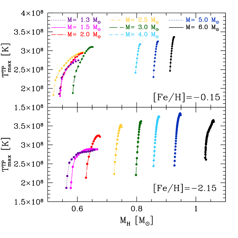
Figure 10: As in Figure 3, but for the maximum temperature attained at the bottom of the convective zone generated by a TP.

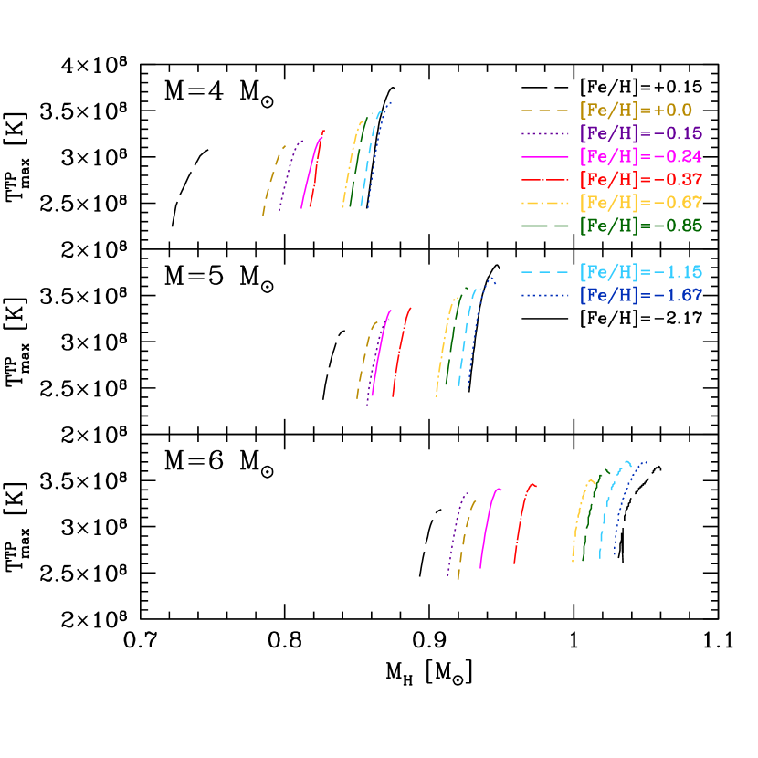
Figure 11: As in Figure 5, but for the maximum temperature attained at the bottom of the convective zone generated by a TP.

Another interesting feature of IMS-AGB models is the large temperature reached at the bottom of the convective shells generated by TPs (T${}^{\rm TP}_{\rm max}$). Depending on T${}^{\rm TP}_{\rm max}$, the ²²Ne($\alpha$,n)²⁵Mg reaction can be efficiently activated. This can lead to a second neutron burst (additional to that from the ¹³C($\alpha$,n)¹⁶O reaction), with important consequences on the s-process nucleosynthesis (see §6). From an inspection of Figures 10 and 11, it can be noticed that, during the AGB, T${}^{\rm TP}_{\rm max}$ progressively increases, reaches a maximum, and then slightly decreases. This quantity depends on the core mass, the envelope mass and the metallicity (see Straniero et al. 2003a). As T${}^{\rm TP}_{\rm max}$ scales with the core mass, we expect the largest temperatures to be attained in the models with the largest initial masses. This is clearly shown in Figure 10, where it can be assessed that low mass stars barely reach T${}^{\rm TP}_{\rm max}\sim 3\times 10^{8}$ K, while IMS-AGB easily go beyond this limit. The dependence on the initial metallicity is also evident, the models with low Z showing definitely larger T${}^{\rm TP}_{\rm max}$ (up to $3.8\times 10^{8}$K) with respect to their solar-like metallicity counterpart. At [Fe/H]=-2.15 the absolute maximum temperature is reached in the 5 M_⊙ model and not in the 6 M_⊙ one. In this case, a larger mass of the H-exhausted core (which implies higher T${}^{\rm TP}_{\rm max}$) can not compensate the decrease of the duration of the interpulse phases.

5 ph-FRUITY: a new web physical interface

The FRUITY database (Cristallo et al., 2011) is organized under a relational model through the MySQL Database Management System. Its Web interface allows users to submit the query strings resulting from filling out appropriately the fields to the managing system, specifying the initial mass, metallicity and rotational velocity. Up to date, FRUITY was including our predictions for the surface composition of AGB stars and the stellar yields they produce. For each model, different types of Tables can be downloaded (elemental and isotopic surface compositions; net and total yields; s-process indexes). In this work, we add a new module (ph-FRUITY), containing the physical quantities of interest characterizing AGB models. The downloadable quantities (given for each Thermal Pulse, with and without TDU) are: the absolute age, the duration of the previous interpulse phase ($\Delta t_{\rm ip}$), the total mass (M_tot), the mass of the H-exhausted core (M_H), the dredged up mass ($\delta$M_TDU), the $\lambda$ quantity, the maximum temperature attained at the bottom of the convective zone generated by the TP (T${}^{\rm TP}_{\rm max}$), the mean bolometric magnitude of the previous interpulse period ($M_{\rm bol}=4.75-2.5*\log$ L/L_⊙), the logarithm of the mean surface temperature of the previous interpulse period (log T_eff) and, the logarithm of the mean surface gravity of the previous interpulse period (log $g$). Note that we stop the calculations once the TDU has ceased to operate. However, the core mass continues to grow up to the nearly complete erosion of the convective envelope by the strong stellar winds. Such an occurrence is accounted for by providing a set of key extrapolated physical quantities (labelled as EXTRA). First, we calculate the mass lost in the wind and the growth of the H-exhausted core during the previous interpulse phase. Then we extrapolate them by means of a 5^th order polynomial. Then, we derive other tabulated quantities ($\Delta t_{\rm ip}$, $M_{\rm bol}$, log T_eff and, log $g$). Following the original FRUITY philosophy, those quantities can be downloaded in a “Multiple case format” (the query returns multiple tables, depending on the number of selected models) or in a “Single case format” (the query returns a single table containing all the selected models).

6 The TP-AGB phase (II): nucleosynthesis

The nucleosynthesis occurring during the TP-AGB phase is extremely rich. In fact, many types of nuclear processes are at work, including strong force reactions (proton captures, neutron captures, $\alpha$ captures) and weak force reactions ($\beta$ decays, electron captures). Nearly all the isotopes in the periodic table are affected, apart from Trans-uranic species.

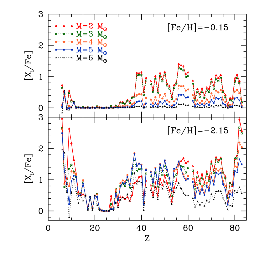
Figure 12: Final element surface distribution for selected masses at solar-like metallicity (upper panel) and at low metallicity (lower panel).

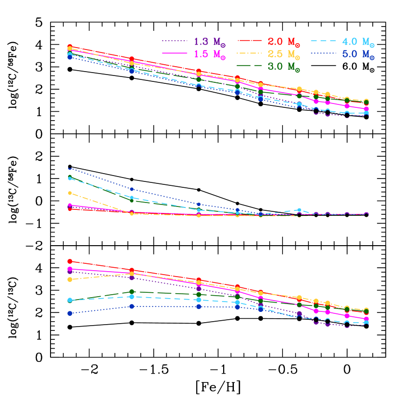
Figure 13: Final surface distributions of ¹²C (upper panel) and ¹³C (intermediate panel) with respect to ⁵⁶Fe as a function of the initial metallicity for the whole FRUITY set. Final surface ¹²C/¹³C ratios are also reported (lower panel).

The nucleosynthetic details related to the evolution of low mass TP-AGB stars have been already presented in Cristallo et al. (2009) and Cristallo et al. (2011). As we already stressed, the final surface abundances and, consequently, the net yields are slightly smaller with respect to data presented in those two papers, due to a previous underestimation of the opacities in the most external layers of the star. The proper opacities imply lower surface temperatures and, thus, higher mass-loss rates. As a consequence, models experience a reduced number of TDU episodes. However, s-process indexes are not affected by this problem (see §6) and, thus, most of the conclusions derived in Cristallo et al. (2011) are still valid.
In Figure 12, we report the final surface chemical distributions for the whole mass range and two selected metallicities (Z=$10^{-2}$: upper panel; Z=$2.4\times 10^{-4}$: lower panel). At large $Z$, we notice a net production of carbon in LMS-AGBs only. The 4 and 5 M_⊙ models present a slight final surface increase, while the 6 M_⊙ model destroys it (due to the occurrence of the FDU, the SDU and to a low TDU efficiency). At low metallicity all models show a consistent production of ¹²C. In Figure 13, we report the final surface number ratios N(¹²C)/N(⁵⁶Fe) and N(¹³C)/N(⁵⁶Fe) as a function of the initial metallicity for the whole FRUITY set (upper panel and intermediate panel, respectively). There is a clear increase in the ¹²C production as the initial iron content decrease. The same is not true for ¹³C, which is efficiently synthesized by the more massive AGBs and for [Fe/H]$<$-0.5 only. The (¹³C/⁵⁶Fe) ratio is in fact nearly flat for models with M$<$2.5 M_⊙. For larger masses (5-6 M_⊙), instead, there is a net ¹³C production, due to the simultaneous occurrence of HBB and H-TDU. The corresponding increase of ¹⁴N can be visualized in Figure 14 (upper panel), as well as the decrease of the ¹²C/¹³C ratio (lower panel of Figure 13). We remind that the ¹³C production is affected by the presence of non-canonical mixing during the RGB phase, as already stressed in §3.
The solar oxygen abundance mainly consists of ¹⁶O. Its production is null at large metallicities, while there is a net production for the whole mass range at low $Z$, thanks to TDU episodes, which mix to the surface the ¹⁶O. The latter is synthesized by the ¹²C($\alpha$,$\gamma$)¹⁶O reactions during TPs and, lo a lesser extent, by the ¹³C($\alpha$,n)¹⁶O reaction during the radiative ¹³C burning. The other oxygen isotopes (¹⁷O and ¹⁸O) exhibit completely different behaviors. The ¹⁷O abundance results from the equilibrium between the production channel (¹⁶O(p,$\gamma$)¹⁷F($\beta^{+}$)¹⁷O nuclear chain) and the destruction one (¹⁷O(p,$\alpha$)¹⁴N reaction). Its surface abundance depends on the depth of convection in regions with an ¹⁷O profile, i.e. those experiencing an incomplete CNO burning. For a fixed [Fe/H], we find the highest ¹⁶O/¹⁷O for the lowest masses (middle panel in Figure 14), thus confirming the values already reported in the literature (see e.g. Lebzelter et al. 2015). The complex interplay between mixing and burning does not allow to identify a common behavior with the metallicity. However, the models show slightly larger ¹⁶O/¹⁷O ratios at large metallicities. The more neutron rich oxygen isotope (¹⁸O) behaves very differently (see lower panel of 14). This isotope is mainly produced by the ¹⁴N($\alpha$,$\gamma$)¹⁸F($\beta^{+}$)¹⁸O nuclear chain, while it is destroyed by the ¹⁸O(p,$\alpha$)¹⁵N and ¹⁸O($\alpha$,$\gamma$)²²Ne reactions. The ¹⁶O/¹⁸O ratio is nearly constant for all masses and [Fe/H]$\geq$-1.15. At low metallicities, its increase is due to the dredge up of primary ¹⁶O, as explained before. Thus, in our models ¹⁸O is basically untouched. This would not be the case, if we would take into consideration the effects induced by non convective mixing during the RGB and the AGB phases. In fact, it has been demonstrated that the inclusion of this kind of mixing strongly affects the surface ¹⁸O abundance of low mass stars and that this is needed to fit laboratory measurements of oxygen isotopic ratios in pre-solar SiC grains (see Palmerini et al. 2011). Those small dust particles are trapped in primitive meteorites and currently provide the most severe constraints to AGB nucleosynthesis (see e.g. Liu et al. 2014, 2015).
The fluorine nucleosynthesis is extremely complex, since it involves both neutron and proton captures (see Abia et al., 2009, 2010, 2011). ¹⁹F is very sensitive to a variation of the initial stellar mass (see lower panel of Figure 12). Its production basically depends on the amount of ¹⁵N in the He-intershell, which in turn is correlated to the amount of ¹³C in the ashes of the H-burning shell, as well as in the ¹³C pocket (see the discussion in Cristallo et al., 2014). In IMS-AGBs, fluorine production is strongly suppressed due to the reduced contribution from the radiative ¹³C burning and from the increased efficiency of ¹⁹F destruction channels (the ¹⁹F(p,$\alpha$)¹⁶O reaction and, above all, the ¹⁹F($\alpha$,p)²²Ne reaction).
Neon is enhanced in all the models experiencing TDU, due to the dredge up of the freshly synthesized ²²Ne during TPs via a double $\alpha$ capture on the abundant ¹⁴N. Its abundance directly affects the ²³Na nucleosynthesis. In LMS-AGBs, sodium can be synthesized through proton captures during the formation of the ¹³C pocket, as well as through neutron captures during both the radiative burning of the ¹³C pocket and the convective ²²Ne-burning in the convective shells generated by TPs (see Cristallo et al. 2009). This leads to a notable ²³Na surface enhancement, in particular at low metallicities. In more massive stars, the sodium nucleosynthesis is affected by HBB (see, e.g. Ventura & D’Antona, 2006; Karakas & Lattanzio, 2014). In our models, we find a slight increase of the ²³Na surface abundance directly correlated to HBB, which is mildly activated in the more massive low Z models.

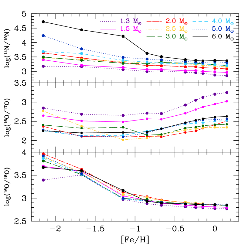
Figure 14: Final surface distributions of the ¹⁴N/¹⁵N ratio (upper panel), the ¹⁶O/¹⁷O ratio (intermediate panel) and, the ¹⁶O/¹⁸O ratio (lower panel).

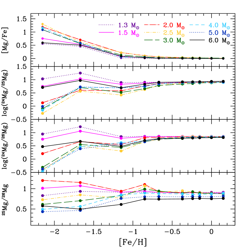
Figure 15: Final surface [Mg/Fe] (upper panel), ²⁴Mg/²⁵Mg and ²⁴Mg/²⁶Mg ratios (intermediate panels) and, ²⁵Mg/²⁶Mg ratio (lower panel).

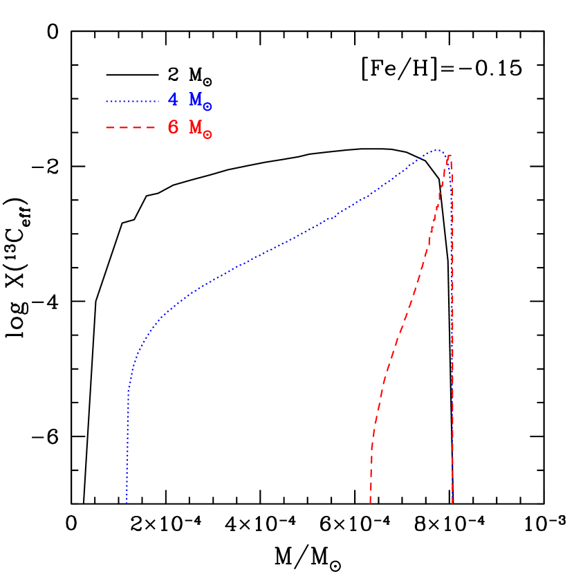
Figure 16: Mass extension of the effective ¹³C in the pockets after the second TDU of the 2.0, 4.0 and, 6.0 M_⊙ models with $Z=10^{-2}$. See text for details.

In our models, magnesium is enhanced at low metallicities, due to an increased production of ²⁵Mg and ²⁶Mg, via the ²²Ne($\alpha$,n)²⁵Mg and the ²²Ne($\alpha$,$\gamma$)²⁵Mg reactions (see upper panel of Figure 15). We find a considerable Mg overabundance at [Fe/H]=-2.15 only (we remind that for [Fe/H]$\leq$-1.67 we adopt an $\alpha$-enhanced initial mixture). At low metallicities both the ²⁴Mg/²⁵Mg and the ²⁴Mg/²⁶Mg are lower than solar (intermediate panels of Figure 15). Both quantities show a minimum for models with initial mass M$\sim$3 M_⊙. Exceptions are represented by the less massive models (1.3 M_⊙ and 1.5 M_⊙), in which the marginal activation of both the ²²Ne($\alpha$,n)²⁵Mg and the ²²Ne($\alpha$,$\gamma$)²⁵Mg reactions does not compensate the initial ²⁴Mg enhancement. At intermediate-to-high metallicities the final surface ²⁶Mg/²⁵Mg ratio of our models is nearly constant (and close to the solar value). At low [Fe/H], instead, it depends on the initial mass, the 2 M_⊙ showing the maximum value and the 5 M_⊙ the minimum one (see lower panel of Figure 15). During TPs, in the massive models the neutron density is large and ²⁵Mg behaves as a neutron poison, thus feeding ²⁶Mg.

The contribution to the overall nucleosynthesis from the ¹³C($\alpha$,n)¹⁶O reaction is strongly correlated to the initial mass of the model. In Cristallo et al. (2009), we showed that the mass extension of the ¹³C pocket decreases with the TDU number (see also Figure 1 in Cristallo et al. 2011), implying a progressive reduction of the s-process efficiency as the star evolves along the AGB. The larger the core mass, the lower the ¹³C size. Thus, ¹³C pockets in IMS-AGB models are definitely thinner with respect to those found in LMS-AGBs, due to their definitely larger core masses. In Figure 16, we compare the profiles of the effective ¹³C (defined as X(¹³C_eff) = X(¹³C) - 13/14 * X(¹⁴N)) in the pocket after the $2^{nd}$ TDU for three different models (2.0, 4.0 and, 6.0 M_⊙) with $Z=10^{-2}$. This quantity takes into account the poisoning effect of ¹⁴N (via the ¹⁴N(n,p)¹⁴C reaction) and, thus, provides a better estimate of the neutrons effectively contributing to the synthesis of heavy elements (see Cristallo et al. 2009).

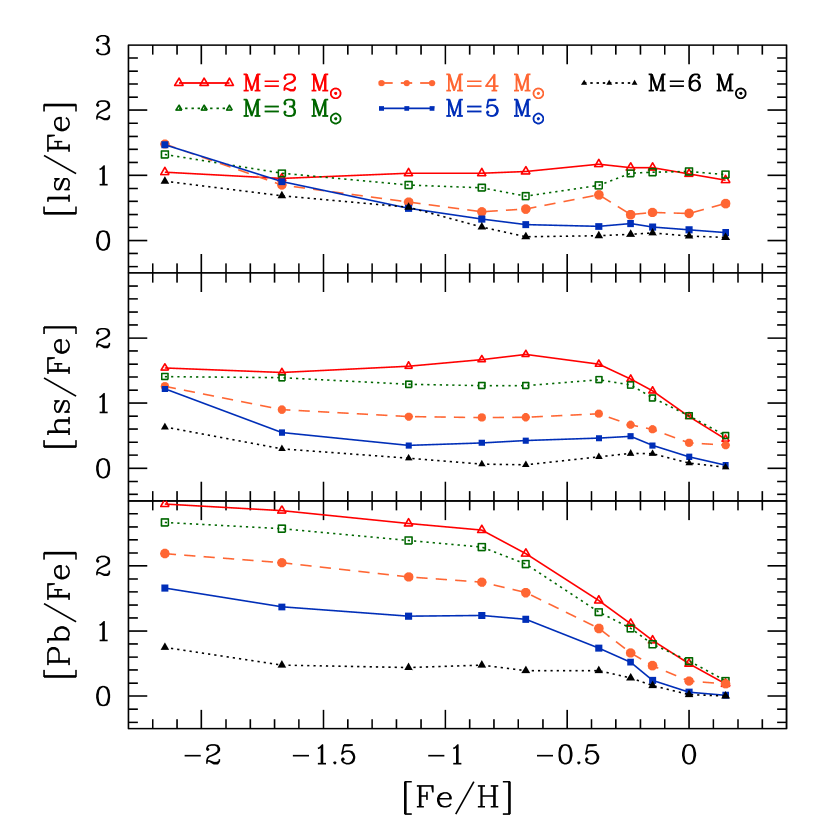
Figure 17: Final surface s-process enhancements: ls component (upper panel), hs component (middle panel) and, lead (lower panel).

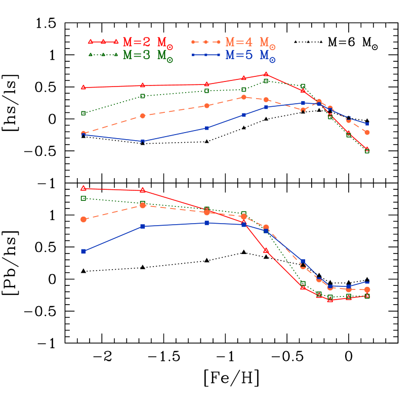
Figure 18: Final surface s-process indexes: [hs/ls] (upper panel) and [Pb/hs] (lower panel).

In Figure 16, the pockets have been manually shifted in mass, while the zero point of the abscissa is arbitrary. The pocket found in the 6 M_⊙ model is four times smaller than that found in the 2 M_⊙ model, due to the shrinking of the He-intershell with increasing initial stellar mass. Moreover, the integrated amount of effective ¹³C in the pocket decreases by more than a factor of 3, passing from the 2 M _⊙ model ($\sum^{13}$C${}_{\rm eff}=7.8\times 10^{-6}$ M_⊙) to the 4 M_⊙ model ($\sum^{13}$C${}_{\rm eff}=2.2\times 10^{-6}$ M_⊙) and is reduced by another factor of 7 in the 6 M_⊙ model ($\sum^{13}$C${}_{\rm eff}=3.1\times 10^{-7}$ M_⊙). This fact has obvious consequences on the production of s-process elements. The main neutron source in LMS-AGBs is the ¹³C($\alpha$,n)¹⁶O reaction (Gallino et al., 1998; Straniero et al., 2006). In those stars, a marginal contribution comes from the partial activation of the ²²Ne($\alpha$,n)²⁵Mg reaction. In Cristallo et al. (2011), we extensively described the final s-process surface distributions for AGB stars in this mass range. Their heavy element distributions show a progressive drift to heavier nuclei as the metallicity decreases. This is due to the fact that the neutron source (the ¹³C($\alpha$,n)¹⁶O reaction) is of primary origin, while the seeds (⁵⁶Fe) scale with metallicity. As a consequence, the lower the initial iron content, the larger the neutron-to-seed ratio. In IMS-AGBs stars, this scheme still holds, but with important differences. As already stressed in Straniero et al. (2014), these objects develop larger temperatures at the base of convective shells during TPs, thus efficiently activating the ²²Ne($\alpha$,n)²⁵Mg reaction. Moreover, the contribution from the ¹³C($\alpha$,n)¹⁶O reaction is lower, due to thinner ¹³C pockets, as shown before. A clear sign of the ²²Ne($\alpha$,n)²⁵Mg activation is reflected in the rubidium surface enhancement (see lower panel of Figure 12). It comes from the large production of ⁸⁷Rb, which is by-passed during the radiative ¹³C burning, due to the branchings at ⁸⁵Kr and, to a lesser extent, at ⁸⁶Rb (Straniero et al., 2014). Since the neutron exposure during the ²²Ne($\alpha$,n)²⁵Mg episode is lower with respect to that of the ¹³C($\alpha$,n)¹⁶O reaction, we also expect an overall reduction of s-process overabundances, in particular for the second and third peak of the s-process. This is confirmed by Figure 17, in which we report the behavior of the three s-process peaks as a function of the metallicity. The corresponding data are tabulated in Tables 14, 15 and, 16. IMS-AGBs show definitely lower surface enhancements for the hs component (intermediate panel) and lead (lower panel). Note that this is also due to the reduced TDU efficiency characterizing those models (see §4). However, at low metallicities the ls component (upper panel) of these models is comparable to that of less massive objects, thus demonstrating that the ²²Ne($\alpha$,n)²⁵Mg reaction is efficiently at work. In a convective environment, neutrons cannot be released and piled up to synthesize the heaviest elements. This is particularly evident for lead, whose production is hampered in IMS-AGBs. The corresponding s-process indexes [hs/ls] and [Pb/hs] are reported in Figure 18. The corresponding data are tabulated in Tables 17 and 18. As already anticipated in previous Sections, we find a general reduction of the surface enhancements with respect to yields from Cristallo et al. (2011). However, the [hs/ls] and [Pb/hs] indexes remain almost unaltered because in LMS-AGBs models those quantities are nearly independent on the evolutionary stage along the AGB, provided that the s-process enhancement is sufficiently large. As already stressed, this derives from the fact that the first ¹³C pockets (the largest ones) are those governing the whole nucleosynthesis. Cristallo et al. (2015) recently computed the galactic chemical evolution of s-only isotopes and found that FRUITY models predict too large abundances for those nuclei. Thus, the reduction of LMS-AGBs yields we discussed in this paper may lead to a better agreement with the observed solar s-only distribution. This problem will be addressed in a forthcoming paper.
The behavior of the [hs/ls] index strongly depends on the initial stellar mass. In fact, the efficient activation of the ²²Ne($\alpha$,n)²⁵Mg reaction and the reduced contribution from the ¹³C($\alpha$,n)¹⁶O reaction lead, in IMS-AGBs, to low [hs/ls] and [Pb/hs] indexes (see Figure 18). Another striking difference with respect to LMS-AGBs is that our massive AGBs do not reach an asymptotic value in the surface ratio between s-process peaks. This can be appreciated in Figure 19, where we plot the [hs/ls] (upper panel) and [Pb/hs] (lower panel) as a function of the TDU number for selected masses with $Z=2.3\times 10^{-4}$. In LMS-AGBs, those quantities rapidly grow up to an asymptotic value and then remain basically frozen (see the 2 M_⊙ curve). For larger masses, instead, both indexes reach a maximum and then start decreasing. This behavior is determined by the additional contribution from the ²²Ne($\alpha$,n)²⁵Mg reaction, which is able to synthesize ls elements, but not to produce the hs ones. Unlike the ¹³C pockets, the imprint of this neutron source progressively emerges with the TDU number. This is due to the fact that the largest temperatures are attained at the base of the convective shells generated by TPs toward the end of the AGB phase (see Figures 10 and 11). The larger the initial mass, the larger the TDU number needed to achieve such an asymptotic regime. The [Pb/hs] does not depend on the activation of the ²²Ne($\alpha$,n)²⁵Mg source, but only on the ¹³C($\alpha$,n)¹⁶O one. Thus, the difference between LMS and IMS is less evident. Obviously, the larger the initial mass, the lower the [Pb/hs] value, due to the decreasing contribution from the ¹³C pockets.

Figure 19: [hs/ls] (upper panel) and [Pb/hs] (lower panel) as a function of the TDU numbers for selected models with [Fe/H]=-2.15.

7 Discussion and Conclusions

A detailed comparison between our LMS-AGB models and those from other groups have been already presented in Cristallo et al. (2011) (see Section 5 of that paper). A similar analysis, but for IMS-AGBs, can be found in Ventura et al. (2013), who compared their models with those published by Karakas (2010), as well as in Fishlock et al. (2014), who made a comparison with a subset of models presented by Straniero et al. (2014). Notwithstanding, in Table 19 we report key quantities related to our 5 M_⊙ model with $Z=1\times 10^{-3}$ compared to similar available models in the literature (Fishlock et al., 2014; Ventura & D’Antona, 2008). Note that there are other published papers on IMS-AGBs; however, they concentrate on different mass regimes (e.g. Siess 2007; Doherty et al. 2015) or present sets for a single metallicity (Herwig 2004). In general, this kind of comparison is not straightforward, since evolutionary codes significantly differ in the adopted input physics (the treatment of convection and convective borders; the mass-loss rate; the initial chemical distribution; the opacities; the equation of state; the nuclear network; etc). For instance, a direct comparison between our models and those presented by Ventura & D’Antona (2008) is difficult because not only the treatment of convective borders is different, but also the theoretical recipe to model convection is not the same (we use the MLT formulation by Cox 1968, while Ventura & D’Antona 2008 adopt the Full Spectrum of Turbulence of Canuto & Mazzitelli 1991). Other differences are the adopted mass-loss rate (Ventura & D’Antona (2008) use a calibrated version of the Bloecker (1995) mass-loss formula) as well as the initial chemical distribution (Ventura & D’Antona (2008) adopt the solar mixture by Grevesse & Sauval (1998) with an $\alpha$ element enhancement of 0.4). From an inspection of Table 19 it turns out that our model shows a HBB shallower than the model by Ventura & D’Antona (2008). It has to be remarked that in the models by Ventura & D’Antona (2008) mixing and burning are coupled. As already stressed, we aim to verify the effects of such a coupling in our models in a future work. Actually, due to the adopted input physics (MLT for convection and mass-loss rate calibrated on galactic AGB stars), our model should be more similar to that of Fishlock et al. (2014). However, also in this case the differences are notable. At odds with our model, the 5 M_⊙ model of Fishlock et al. (2014) experience a stronger HBB (as testified by the large temperatures attained at the base of the convective envelope during interpulse periods). In our models, we test the effects of changing the efficiency of mixing (we vary the free parameter of the MLT or the $\beta$ parameter governing the convective velocity profile at the base of the convective envelope), the mixing scheme (by assuming instantaneous mixing in the envelope), the treatment of opacities at the border of the convective envelope, the adopted mass-loss rate (we run a model without mass-loss and let it to evolve to larger core masses) or the equation of state (EOS; we substitute our treatment by adopting the OPAL EOS 2005 at high temperatures (Rogers et al., 1996) and checking different transition temperatures to the low temperature regime). Those test lead to variations of the ¹²C/¹³C ratio, but none of them shows a significant activation of HBB. Thus, we are not able to explain such a discrepancy in the thermal stratification of our models with respect to Fishlock et al. (2014). Perhaps the origin has to be searched in the dated EOS used by Fishlock et al. (2014). As reported in Doherty et al. (2015), the perfect gas equation is adopted for fully ionized regions, the Saha EOS in partially ionized regions (following the method of Bærentzen 1965), while EOS from Beaudet & Tassoul (1971) is used for relativistic or electron-degenerate gas. However, a discussion on the proper EOS to be used in AGB stellar models, as well on the effects induced by adopting different EOS, is beyond the goals of this paper.
More meaningful conclusions can be derived by comparing theoretical models to observed quantities. As discussed in §4, the majority of our models present final C/O ratios larger than 1. Their observational counterparts are C-rich stars, whose Luminosity Function, which links a physical quantity (the luminosity) with the chemistry (its surface carbon abundance), represents a good test indicator for theoretical prescriptions. A revision of the observational galactic Luminosity Function of Carbon Stars (LFCS) has been recently presented by Guandalini & Cristallo (2013). Such a LFCS is plotted in Figure 20 (dotted histogram), together with the theoretical LFCS obtained with models by Cristallo et al. (2011) (dashed histogram) and with models presented in this paper (continuous histogram). With respect to our previous estimate, we note a marginal shift to low luminosities, as a consequence of the reduced TP-AGB lifetimes caused by the erroneous treatment in the opacities of the most external layers of the star. In the upper right corner of Figure 20 we report the LFCS derived by considering the contribution of IMS-AGBs only. Those objects populate the high luminosity tail of the LFCS. However, their contribution to the whole distribution is practically negligible. Thus, at variance with LMS-AGBs, the LFCS cannot be fruitfully used to constrain the physical evolution of IMS-AGBs.

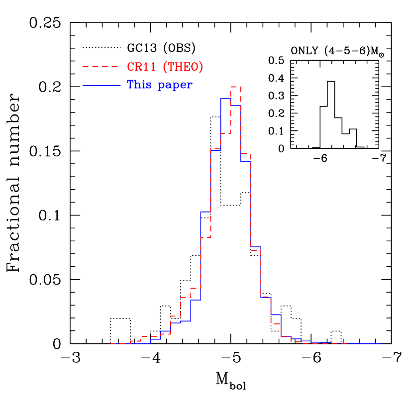
Figure 20: Our new theoretical Luminosity Function of Carbon Stars (solid curve) compared to our previous estimate (dashed curve; CR11: Cristallo et al. 2011) and to observations (dashed curve; GC13: Guandalini & Cristallo 2013).

Another interesting quantity, which can be used to constrain theoretical models, is the initial-to-final mass relation. This relation depends on the core mass of the H-exhausted core attained at the end of the TP-AGB phase. As already recalled in §4, for the more massive models presented here the presence of the SDU induces important variations in the mass of the H-exhausted core. In Figure 21 we compare a selection of our models to the semi-empirical initial-to-final mass relation of Weidemann (2000) as well as to observational data of Open Clusters (Ferrario et al., 2005; Catalán et al., 2008; Dobbie et al., 2009; Williams et al., 2009; Zhao et al., 2012; Kalirai et al., 2014). In Table 20 we report the final core masses of the whole FRUITY set.

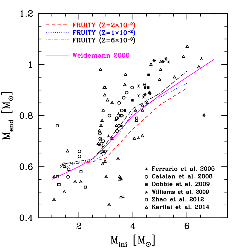
Figure 21: FRUITY models Initial-to-final mass relations for selected metallicities, compared to the semi-empirical relation from Weidemann (2000) and to Open Clusters observations.

Our theoretical models agree well with the semi-empirical initial-to-final mass relation of Weidemann (2000), showing however larger core masses for low mass objects. When looking to observations, the situation becomes more complex. For a fixed initial mass, observations present a rather wide spread up to $\sim 0.5$ M_⊙. Thus, firm conclusions cannot be drawn. Moreover, it has to be taken into account that many observations are indirectly affected by the uncertainty characterizing stellar models. In fact, while the WD mass can be determined basing on spectroscopic data, the initial mass is generally derived by estimating the cluster age. This evaluation is done by means of theoretical relations among mass, age and turn off luminosity. Thus, the result depends on the physical recipe adopted to compute the cluster isocrone. In Figure 21 we report core masses at the last computed model (i.e. when TDU ceases to operate). The computing of the following evolutionary phases is made difficult by the treatment of the most external layers. The final surface chemistry remains frozen up to the WD phase, unless a very Late Thermal Pulse occurs (Iben et al., 1983; Herwig et al., 2011). Note that only under the hypothesis of a strong final super-wind episode, able to instantaneously remove the whole remaining envelope, core masses at the last TDU would coincide with WD masses. Alternatively, the star experiences additional TPs without TDU up to the almost complete erosion of the convective envelope. Then, we also performed an extrapolation of the core mass. For models with an initial mass larger than 3 M_⊙, the differences in the core mass between the last computed model and the extrapolated number are neglibile (lower than 0.01 M_⊙), while in the LMS regime they become appreciable (up to 0.035 M_⊙). The extrapolated final masses are reported in the ph-FRUITY database.
Spectroscopic observations, able to constrain the evolution of IMS-AGBs, are rare. The lack of C-stars in Magellanic Clouds (MCs) with luminosities larger than M_bol=-6 led Wood et al. (1983) to the conclusion that CNO cycling is at work in upper AGB stars, preventing them to become C-rich. Actually, it cannot be excluded that C-rich stars with high luminosities exist, since they could be embedded in an opaque dust rich cloud masking them to observations. For instance, van Loon et al. (1999) found giant C-rich stars up to M_bol=-6.7, thus demonstrating that in those objects TDU is at work and that HBB is not efficient enough to make those stars O-rich. More recently, a restricted sample of galactic O-rich giant stars has been presented by García-Hernández et al. (2006). Unfortunately, in the spectral regions under analysis, the adopted synthetic spectra do not have the necessary resolution to precisely fix the carbon, nitrogen, and oxygen abundances (as well as the ¹²C/¹³C ratio, see García-Hernández et al. 2007). Moreover, for galactic stars the determination of the absolute magnitude is highly uncertain due to the difficulties in determining the distance of those objects. Thus, apart from the derived C/O ratio (less than 0.75) and the lithium abundance, they cannot be used to constrain HBB. However, our models can be tested by checking their s-process elements abundances. Stars observed by García-Hernández et al. (2006) have been found extremely rubidium-rich and zirconium poor. This is at odds with theoretical s-process expectations. However, more recently the same authors (Zamora et al., 2014) re-analyzed 4 stars demonstrating that the inclusion of a circum-stellar component leads to definitely lower Rb surface abundances, without appreciably modifying Zr data. Looking to their Table 1, we notice that for the galactic sample all stars are compatible, within errors, with null s-process enrichments (for both Rb and Zr) but IRAS 18429-1721, showing an appreciable Rb enrichment ([Rb/M]=1.0$\pm$0.4). A more trustful comparison could be made with a similar sample, but for stars belonging to MCs (García-Hernández et al., 2009). In that case, distances are better known and bolometric magnitudes can be derived. On average, stars are Zr-poor (some of them showing some enhancement) and, thus, agree with our models. Those objects are Rb-rich. However, as for the galactic sample, a decrease in the Rb abundance is expected when considering a circum-stellar component, as demonstrated by the LMC star (IRAS 04498-6842; Zamora et al. 2014). The rubidium surface enrichment of this star ([Rb/M]=1.5$\pm$0.7) is not in agreement with our models, even when taking into account the large observational errors. Its bolometric magnitude ($M_{\rm bol}$=-7.72) may indicate a larger stellar mass with respect to those presented in this paper. At the same time, however, it could be the proof of the activation of HBB, which implies larger surface luminosities with respect to those expected from the core-luminosity relation (see e.g. Bloecker & Schoenberner 1991). In conclusion, apart from one single object, our models do not disagree with the discussed observational data. Another interesting sample is that by McSaveney et al. (2007), who presented C, N, and O abundances in two O-rich luminous Giant belonging to the Large magellanic Cloud (NGC 1866#4 and HV2576). In particular, those authors found a strong carbon depletion ($\sim$ 1 dex) coupled to a clear nitrogen enhancement ($\sim$ 1 dex). They concluded that this is the proof for the occurrence of ongoing HBB in the analyzed stars. However, alternative theories could be explored. First, we remember that, before entering the TP-AGB phase, FDU and SDU increase the surface N abundance by a factor of 3. This is not enough to reproduce observations. However, it has to be stressed that additional physical phenomena may produce similar abundance patterns. An illuminating case is represented by rotation. Models presented in this paper do not take into account the effects of rotation. In Piersanti et al. (2013), we demonstrated that mixing induced by rotation may significantly change the final surface theoretical distributions of LMS-AGB models. Rotation may induce non canonical mixing also in larger masses. In particular, during the Main Sequence phase meridional circulations (von Zeipel, 1924a, b) may work in the layers between the inner border of the convective envelope and the upper border of the receding H-burning convective core. In that case, a mixing would develop in a region that previously experienced CN cycling. Later, after the occurrence of FDU, the surface CN abundances could result varied. We test the effects of rotation on a 6 M_⊙ model with $Z=10^{-2}$ and different initial rotation velocities. We find that models rotating on the Zero Age Main Sequence (ZAMS) with v${}^{\rm ini}_{\rm rot}\sim$100 km/s (thus not so high for stars with this mass) already show a large C depletion (-1 dex) and a strong nitrogen enhancement (+0.7 dex). Note that similar conclusions have already been derived by Georgy et al. (2013), even with a different formulation for the transport of angular momentum.
Other useful constraints to theoretical models come from the study of the abundances derived in Planetary Nebulae (PNe), which lie between the tip of the AGB and the WDs cooling sequence (for a review see Balick & Frank 2002). During that evolutionary phase, the strong mass loss practically peels the H-exhausted core. The star evolves toward higher surface temperatures at almost constant luminosity and, when the ionization of the lost gas begins, a PN emerges. It has been shown (see García-Hernández & Górny 2014 for an updated study) that a consistent fraction of PNe are N-rich (the so-called type I PNe). The most ¹⁴N-enriched PNe are not accessible by our models. However, a considerable fraction of the sample can be reproduced by taking into account the variations in CNO abundances caused by the occurrence of FDU and/or SDU. Moreover, the effects induced by rotation (see above) or the presence of a companion (De Marco, 2009) could complicate the physical and chemical behavior of PNe. Finally, let us stress that a precise determination of the PNe masses is not an easy task (as always for galactic objects). It could be that the most N-rich PNe are the remnant of the evolution of massive AGBs (7-8-9 M_⊙; the so-called super-AGBs), whose evolution is not explored in this paper.
Finally, let us stress that up to date no signature of HBB has been found in pre-solar grains. In 2007, it has been claimed that the composition of the peculiar spinel grain OC2 could be attributed to the nucleosynthesis induced by HBB in a massive AGB star (Lugaro et al., 2007). However, in order to reconcile theoretical models and laboratory measurements, a modification of nuclear cross sections was needed. Later, the same authors (Iliadis et al., 2008) rejected such an hypothesis, identifying a low mass star experiencing additional non convective mixing as the best candidate to explain the isotopic signatures of that grain (see also Palmerini et al. 2013). This does not necessarily imply that pre-solar SiC grains carrying the signature of HBB do not exist, but that they have not been discovered yet.

Table 1: Initial helium and $\alpha$ enrichment for different initial masses and metallicities. Bold labels refer to models added with this work.

Mass$\diagup$Z	$2.4\times 10^{-4}$	$7.2\times 10^{-4}$	$1.0\times 10^{-3}$	$2.0\times 10^{-3}$	$3.0\times 10^{-3}$	$6.0\times 10^{-3}$	$8.0\times 10^{-3}$	$1.0\times 10^{-2}$	$1.4\times 10^{-2}$	$2.0\times 10^{-2}$
Mass$\diagup$[Fe/H]	-2.15	-1.67	-1.15	-0.85	-0.67	-0.37	-0.24	-0.15	0.00	0.15
1.3	(0.245;0.5)	(0.245;0.5)	(0.245;0)	(0.252;0)	(0.260;0)	(0.260;0)	(0.265;0)	(0.265;0)	(0.269;0)	(0.269;0)
1.5	(0.245;0.5)	(0.245;0.5)	(0.245;0)	(0.252;0)	(0.260;0)	(0.260;0)	(0.265;0)	(0.265;0)	(0.269;0)	(0.269;0)
2.0	(0.245;0.5)	(0.245;0.5)	(0.245;0)	(0.252;0)	(0.260;0)	(0.260;0)	(0.265;0)	(0.265;0)	(0.269;0)	(0.269;0)
2.5	(0.245;0.5)	(0.245;0.5)	(0.245;0)	(0.252;0)	(0.260;0)	(0.260;0)	(0.265;0)	(0.265;0)	(0.269;0)	(0.269;0)
3.0	(0.245;0.5)	(0.245;0.5)	(0.245;0)	(0.252;0)	(0.260;0)	(0.260;0)	(0.265;0)	(0.265;0)	(0.269;0)	(0.269;0)
4.0	(0.245;0.5)	(0.245;0.5)	(0.245;0)	(0.252;0)	(0.260;0)	(0.260;0)	(0.265;0)	(0.265;0)	(0.269;0)	(0.269;0)
5.0	(0.245;0.5)	(0.245;0.5)	(0.245;0)	(0.252;0)	(0.260;0)	(0.260;0)	(0.265;0)	(0.265;0)	(0.269;0)	(0.269;0)
6.0	(0.245;0.5)	(0.245;0.5)	(0.245;0)	(0.252;0)	(0.260;0)	(0.260;0)	(0.265;0)	(0.265;0)	(0.269;0)	(0.269;0)

Table 2: Main Sequence lifetimes (yr) for different initial masses and metallicities.

Mass$\diagup$[Fe/H]	-2.15	-1.67	-1.15	-0.85	-0.67	-0.37	-0.24	-0.15	0.00	0.15
1.3	2.38E+09	2.38E+09	2.45E+09	2.50E+09	2.53E+09	2.95E+09	3.15E+09	3.49E+09	3.75E+09	4.76E+09
1.5	1.51E+09	1.51E+09	1.56E+09	1.60E+09	1.61E+09	1.85E+09	1.98E+09	2.16E+09	2.31E+09	2.84E+09
2.0	6.25E+08	6.51E+08	6.80E+08	7.12E+08	7.12E+08	8.10E+08	8.44E+08	9.13E+08	9.70E+08	1.16E+09
2.5	3.44E+08	3.60E+08	3.75E+08	3.88E+08	3.82E+08	4.30E+08	4.47E+08	4.79E+08	5.03E+08	5.92E+08
3.0	2.20E+08	2.28E+08	2.35E+08	2.42E+08	2.38E+08	2.64E+08	2.71E+08	2.88E+08	2.99E+08	3.46E+08
4.0	1.14E+08	1.16E+08	1.20E+08	1.20E+08	1.19E+08	1.29E+08	1.32E+08	1.39E+08	1.44E+08	1.66E+08
5.0	7.11E+07	7.17E+07	7.30E+07	7.23E+07	7.11E+07	7.53E+07	7.65E+07	7.97E+07	8.19E+07	9.10E+07
6.0	4.95E+07	4.95E+07	4.98E+07	4.91E+07	4.80E+07	5.03E+07	5.07E+07	5.24E+07	5.34E+07	5.80E+07

Table 3: Maximum size of the convective core developed during the MS (in solar units).

Mass$\diagup$[Fe/H]	-2.15	-1.67	-1.15	-0.85	-0.67	-0.37	-0.24	-0.15	0.00	0.15
1.3	0.147	0.130	0.130	0.111	0.120	0.155	0.164	0.155	0.164	0.155
1.5	0.211	0.200	0.189	0.169	0.169	0.147	0.141	0.136	0.131	0.122
2.0	0.386	0.376	0.365	0.346	0.336	0.327	0.310	0.301	0.293	0.270
2.5	0.569	0.553	0.538	0.524	0.509	0.496	0.483	0.496	0.469	0.444
3.0	0.783	0.761	0.741	0.721	0.702	0.664	0.663	0.646	0.628	0.594
4.0	1.198	1.198	1.133	1.074	1.045	1.015	0.987	0.962	0.962	0.988
5.0	1.606	1.606	1.538	1.457	1.417	1.342	1.342	1.342	1.269	1.342
6.0	2.043	2.043	1.928	1.846	1.797	1.700	1.700	1.700	1.610	1.700

Table 4: The H-exhausted core mass at the beginning of the He burning (in solar units).

Mass$\diagup$[Fe/H]	-2.15	-1.67	-1.15	-0.85	-0.67	-0.37	-0.24	-0.15	0.00	0.15
1.3	0.485	0.487	0.488	0.487	0.485	0.485	0.490	0.490	0.481	0.480
1.5	0.473	0.482	0.484	0.484	0.484	0.484	0.483	0.483	0.481	0.480
2.0	0.404	0.437	0.452	0.451	0.451	0.462	0.463	0.466	0.465	0.471
2.5	0.347	0.344	0.343	0.341	0.324	0.317	0.319	0.317	0.315	0.314
3.0	0.405	0.400	0.397	0.393	0.383	0.383	0.382	0.378	0.375	0.369
4.0	0.533	0.533	0.525	0.518	0.518	0.506	0.504	0.498	0.494	0.484
5.0	0.675	0.666	0.675	0.656	0.656	0.639	0.635	0.630	0.626	0.618
6.0	0.822	0.822	0.822	0.799	0.799	0.782	0.777	0.766	0.766	0.756

Table 5: Central helium burning lifetimes (yr) for different initial masses and metallicities.

Mass$\diagup$[Fe/H]	-2.15	-1.67	-1.15	-0.85	-0.67	-0.37	-0.24	-0.15	0.00	0.15
1.3	8.72E+07	8.95E+07	9.06E+07	9.39E+07	9.64E+07	1.01E+08	9.16E+07	9.23E+07	1.10E+08	1.17E+08
1.5	9.16E+07	9.02E+07	9.08E+07	9.35E+07	9.57E+07	1.00E+06	1.03E+08	1.05E+08	1.09E+08	1.16E+08
2.0	1.13E+08	1.04E+08	1.02E+08	1.11E+08	1.14E+08	1.14E+08	1.16E+08	1.17E+08	1.19E+08	1.22E+08
2.5	9.68E+07	1.11E+08	1.23E+08	1.36E+08	1.51E+08	1.99E+08	2.18E+08	2.42E+08	2.59E+08	3.02E+08
3.0	5.87E+07	6.45E+07	7.05E+07	7.70E+07	7.96E+07	9.75E+07	1.10E+08	1.25E+08	1.38E+08	1.68E+08
4.0	2.67E+07	2.81E+07	3.02E+07	3.28E+07	3.41E+07	3.79E+07	3.92E+07	4.21E+07	4.54E+07	5.68E+07
5.0	1.50E+07	1.56E+07	1.66E+07	1.80E+07	1.87E+07	2.06E+07	2.09E+07	2.19E+07	2.21E+07	2.47E+07
6.0	9.55E+06	9.94E+06	1.04E+07	1.12E+07	1.16E+07	1.28E+07	1.29E+07	1.31E+07	1.34E+07	1.44E+07

Table 6: The H-exhausted core mass at the end of the He burning (in solar units).

Mass$\diagup$[Fe/H]	-2.15	-1.67	-1.15	-0.85	-0.67	-0.37	-0.24	-0.15	0.00	0.15
1.3	0.551	0.548	0.544	0.540	0.538	0.533	0.531	0.528	0.527	0.523
1.5	0.567	0.561	0.553	0.547	0.545	0.537	0.535	0.532	0.531	0.525
2.0	0.616	0.604	0.588	0.556	0.550	0.539	0.534	0.531	0.531	0.527
2.5	0.716	0.684	0.660	0.621	0.595	0.531	0.517	0.506	0.506	0.489
3.0	0.819	0.797	0.775	0.736	0.717	0.642	0.607	0.577	0.562	0.536
4.0	1.055	1.045	1.026	0.991	0.968	0.888	0.862	0.824	0.793	0.715
5.0	1.324	1.319	1.300	1.269	1.247	1.133	1.075	1.066	1.052	0.976
6.0	1.610	1.600	1.578	1.556	1.534	1.423	1.355	1.286	1.325	1.245

Table 7: The total stellar mass at the beginning of the AGB phase (in solar units).

Mass$\diagup$[Fe/H]	-2.15	-1.67	-1.15	-0.85	-0.67	-0.37	-0.24	-0.15	0.00	0.15
1.3	1.203	1.187	1.177	1.165	1.157	1.134	1.124	1.117	1.109	1.091
1.5	1.422	1.405	1.398	1.388	1.379	1.362	1.354	1.350	1.343	1.330
2.0	1.956	1.942	1.938	1.941	1.938	1.928	1.921	1.915	1.917	1.899
2.5	2.458	2.456	2.457	2.461	2.466	2.477	2.478	2.479	2.475	2.473
3.0	2.957	2.949	2.948	2.950	2.949	2.963	2.969	2.976	2.978	2.981
4.0	3.963	3.943	3.920	3.894	3.837	3.785	3.768	3.807	3.822	3.940
5.0	4.952	4.909	4.862	4.800	4.713	4.578	4.599	4.556	4.516	4.517
6.0	5.886	5.797	5.772	5.645	5.467	5.203	5.203	5.266	5.103	4.970

Table 8: The H-exhausted core mass at the beginning of the AGB phase (in solar units).

Mass$\diagup$[Fe/H]	-2.15	-1.67	-1.15	-0.85	-0.67	-0.37	-0.24	-0.15	0.00	0.15
1.3	0.563	0.559	0.554	0.551	0.550	0.543	0.541	0.538	0.539	0.534
1.5	0.578	0.572	0.564	0.557	0.555	0.547	0.545	0.543	0.542	0.536
2.0	0.629	0.615	0.596	0.566	0.557	0.545	0.543	0.541	0.541	0.538
2.5	0.724	0.697	0.670	0.633	0.598	0.540	0.528	0.519	0.523	0.517
3.0	0.798	0.795	0.773	0.742	0.721	0.651	0.616	0.585	0.572	0.545
4.0	0.857	0.857	0.853	0.845	0.840	0.817	0.811	0.796	0.785	0.722
5.0	0.928	0.927	0.920	0.912	0.905	0.874	0.861	0.857	0.850	0.826
6.0	1.031	1.028	1.018	1.006	0.999	0.959	0.935	0.913	0.920	0.893

Table 9: Surface mass fractions of selected isotopes for models with $Z=1.0\times 10^{-2}$ at different evolutionary phases (initial, after the FDU, after the SDU).

Isot.	Phase	1.3	1.5	2.0	2.5	3.0	4.0	5.0	6.0
4He	INI	2.65E-01	2.65E-01	2.65E-01	2.65E-01	2.65E-01	2.65E-01	2.65E-01	2.65E-01
4He	FDU	2.88E-01	2.84E-01	2.77E-01	2.79E-01	2.81E-01	2.76E-01	2.71E-01	2.70E-01
4He	SDU	—	—	—	—	—	2.85E-01	3.11E-01	3.31E-01
12C	INI	1.64E-03	1.64E-03	1.64E-03	1.64E-03	1.64E-03	1.64E-03	1.64E-03	1.64E-03
12C	FDU	1.19E-03	1.12E-03	1.01E-03	9.60E-04	9.55E-04	9.72E-04	9.87E-04	9.92E-04
12C	SDU	—	—	—	—	—	9.34E-04	9.13E-04	8.93E-04
13C	INI	1.99E-05	1.99E-05	1.99E-05	1.99E-05	1.99E-05	1.99E-05	1.99E-05	1.99E-05
13C	FDU	4.96E-05	4.95E-05	4.71E-05	4.65E-05	4.61E-05	4.81E-05	4.92E-05	4.97E-05
13C	SDU	—	—	—	—	—	4.81E-05	4.74E-05	4.56E-05
14N	INI	5.31E-04	5.31E-04	5.31E-04	5.31E-04	5.31E-04	5.31E-04	5.31E-04	5.31E-04
14N	FDU	1.02E-03	1.11E-03	1.24E-03	1.43E-03	1.52E-03	1.49E-03	1.42E-03	1.40E-03
14N	SDU	—	—	—	—	—	1.59E-03	1.72E-03	1.89E-03
15N	INI	2.09E-06	2.09E-06	2.09E-06	2.09E-06	2.09E-06	2.09E-06	2.09E-06	2.09E-06
15N	FDU	1.43E-06	1.28E-06	1.04E-06	9.50E-07	9.34E-07	9.97E-07	9.82E-07	9.68E-07
15N	SDU	—	—	—	—	—	9.48E-07	9.03E-07	8.82E-07
16O	INI	4.40E-03	4.40E-03	4.40E-03	4.40E-03	4.40E-03	4.40E-03	4.40E-03	4.40E-03
16O	FDU	4.40E-03	4.39E-03	4.37E-03	4.23E-03	4.13E-03	4.15E-03	4.20E-03	4.23E-03
16O	SDU	—	—	—	—	—	4.09E-03	3.96E-03	3.81E-03
17O	INI	1.74E-06	1.74E-06	1.74E-06	1.74E-06	1.74E-06	1.74E-06	1.74E-06	1.74E-06
17O	FDU	3.20E-06	6.12E-06	2.34E-05	2.23E-05	1.82E-05	1.43E-05	1.26E-05	1.17E-05
17O	SDU	—	—	—	—	—	1.49E-05	1.24E-05	1.10E-05
18O	INI	9.92E-06	9.92E-06	9.92E-06	9.92E-06	9.92E-06	9.92E-06	9.92E-06	9.92E-06
18O	FDU	8.20E-06	7.78E-06	7.08E-06	6.76E-06	6.69E-06	6.58E-06	6.66E-06	6.69E-06
18O	SDU	—	—	—	—	—	6.35E-06	6.16E-06	5.99E-06
23Na	INI	2.58E-05	2.58E-05	2.58E-05	2.58E-05	2.58E-05	2.58E-05	2.58E-05	2.58E-05
23Na	FDU	2.64E-05	2.78E-05	3.18E-05	3.42E-05	3.50E-05	3.47E-05	3.41E-05	3.41E-05
23Na	SDU	—	—	—	—	—	3.60E-05	3.78E-05	4.09E-05

Table 10: Surface mass fractions of selected isotopes for models with $Z=2.3\times 10^{-4}$ at different evolutionary phases (initial, after the FDU, after the SDU).

Isot.	Phase	1.3	1.5	2.0	2.5	3.0	4.0	5.0	6.0
4He	INI	2.45E-01	2.45E-01	2.45E-01	2.45E-01	2.45E-01	2.45E-01	2.45E-01	2.45E-01
4He	FDU	2.68E-01	2.69E-01	2.66E-01	2.46E-01	—	—	—	—
4He	SDU	—	—	—	2.55E-01	2.63E-01	3.03E-01	3.28E-01	3.42E-01
12C	INI	1.68E-05	1.68E-05	1.68E-05	1.68E-05	1.68E-05	1.68E-05	1.68E-05	1.68E-05
12C	FDU	1.13E-05	1.02E-05	8.62E-06	1.44E-05	—	—	—	—
12C	SDU	—	—	—	8.76E-06	8.03E-06	7.13E-06	6.71E-06	1.06E-05
13C	INI	2.04E-07	2.04E-07	2.04E-07	2.04E-07	2.04E-07	2.04E-07	2.04E-07	2.04E-07
13C	FDU	4.93E-07	4.75E-07	4.52E-07	7.55E-07	—	—	—	—
13C	SDU	—	—	—	4.75E-07	4.58E-07	4.41E-07	4.27E-07	4.17E-07
14N	INI	5.44E-06	5.44E-06	5.44E-06	5.44E-06	5.44E-06	5.44E-06	5.44E-06	5.44E-06
14N	FDU	1.16E-05	1.29E-05	1.85E-05	7.60E-06	—	—	—	—
14N	SDU	—	—	—	1.83E-05	2.18E-05	3.16E-05	3.90E-05	4.33E-05
15N	INI	2.14E-08	2.14E-08	2.14E-08	2.14E-08	2.14E-08	2.14E-08	2.14E-08	2.14E-08
15N	FDU	1.38E-08	1.23E-08	1.06E-08	1.41E-08	—	—	—	—
15N	SDU	—	—	—	9.51E-09	8.59E-09	7.59E-09	6.98E-09	6.63E-09
16O	INI	1.42E-04	1.42E-04	1.42E-04	1.42E-04	1.42E-04	1.42E-04	1.42E-04	1.42E-04
16O	FDU	1.42E-04	1.42E-04	1.33E-04	1.42E-04	—	—	—	—
16O	SDU	—	—	—	1.37E-04	1.34E-04	1.23E-04	1.16E-04	1.11E-04
17O	INI	1.79E-08	1.79E-08	1.79E-08	1.79E-08	1.79E-08	1.79E-08	1.79E-08	1.79E-08
17O	FDU	2.18E-07	9.38E-07	2.39E-06	1.85E-08	—	—	—	—
17O	SDU	—	—	—	7.97E-07	1.44E-06	1.98E-06	1.77E-06	1.52E-06
18O	INI	1.02E-07	1.02E-07	1.02E-07	1.02E-07	1.02E-07	1.02E-07	1.02E-07	1.02E-07
18O	FDU	7.59E-08	6.94E-08	5.38E-08	9.70E-08	—	—	—	—
18O	SDU	—	—	—	6.04E-08	5.55E-08	4.88E-08	4.52E-08	8.00E-08
23Na	INI	2.64E-07	2.64E-07	2.64E-07	2.64E-07	2.64E-07	2.64E-07	2.64E-07	2.64E-07
23Na	FDU	2.94E-07	3.35E-07	3.98E-07	2.64E-07	—	—	—	—
23Na	SDU	—	—	—	4.26E-07	7.28E-07	1.69E-06	2.13E-06	2.12E-06

Table 11: Description of dredge up events: first dredge up (F), second dredge up (S) and third dredge ups (T) characterizing models with different masses and metallicities. If the model experience third dredge ups, we report the numbers of experienced episodes.

[Fe/H]	-2.15			-1.67			-1.15			-0.85			-0.67			-0.37			0.24			-0.15			0.00			0.15
Mass	F	S	T	F	S	T	F	S	T	F	S	T	F	S	T	F	S	T	F	S	T	F	S	T	F	S	T	F	S	T
1.3	YES	NO	9	YES	NO	7	YES	NO	5	YES	NO	5	YES	NO	4	YES	NO	3	YES	NO	2	YES	NO	2	YES	NO	NO	YES	NO	NO
1.5	YES	NO	12	YES	NO	9	YES	NO	8	YES	NO	7	YES	NO	6	YES	NO	7	YES	NO	5	YES	NO	4	YES	NO	5	YES	NO	4
2.0	YES	NO	13	YES	NO	13	YES	NO	11	YES	NO	11	YES	NO	11	YES	NO	10	YES	NO	10	YES	NO	9	YES	NO	9	YES	NO	9
2.5	YES	YES	14	YES	YES	11	YES	YES	10	YES	NO	10	YES	YES	11	YES	NO	13	YES	NO	15	YES	NO	14	YES	NO	13	YES	NO	15
3.0	NO	YES	16	YES	YES	13	YES	YES	11	YES	YES	10	YES	YES	9	YES	YES	9	YES	YES	10	YES	NO	11	YES	NO	13	YES	NO	14
4.0	NO	YES	25	YES	YES	19	YES	YES	15	YES	YES	15	YES	YES	12	YES	YES	9	YES	YES	9	YES	YES	8	YES	YES	8	YES	YES	8
5.0	NO	YES	39	NO	YES	32	YES	YES	24	YES	YES	22	YES	YES	18	YES	YES	12	YES	YES	11	YES	YES	11	YES	YES	8	YES	YES	7
6.0	NO	YES	82	NO	YES	66	NO	YES	57	YES	YES	41	YES	YES	31	YES	YES	22	YES	YES	18	YES	YES	16	YES	YES	15	YES	YES	11

Table 12: Cumulative dredged up mass (in M_⊙) for different initial masses and metallicities.

Mass$\diagup$[Fe/H]	-2.15	-1.67	-1.15	-0.85	-0.67	-0.37	-0.24	-0.15	0.00	0.15
1.3	1.36E-02	1.19E-02	9.89E-03	8.64E-03	4.65E-03	2.82E-03	5.75E-04	2.64E-04	0.00E+00	0.00E+00
1.5	3.28E-02	2.83E-02	2.45E-02	2.14E-02	1.64E-02	1.41E-02	8.15E-03	8.46E-03	6.66E-03	5.58E-03
2.0	7.89E-02	6.44E-02	6.54E-02	6.15E-02	5.26E-02	4.61E-02	3.50E-02	3.88E-02	2.91E-02	2.96E-02
2.5	6.61E-02	4.54E-02	5.88E-02	6.12E-02	6.40E-02	8.20E-02	7.23E-02	7.25E-02	5.91E-02	6.67E-02
3.0	4.83E-02	2.95E-02	3.17E-02	3.20E-02	2.72E-02	4.10E-02	4.74E-02	5.77E-02	6.01E-02	6.43E-02
4.0	5.15E-02	3.15E-02	2.17E-02	2.27E-02	1.59E-02	1.53E-02	8.90E-03	8.59E-03	7.28E-03	1.10E-02
5.0	4.31E-02	3.01E-02	2.16E-02	2.15E-02	1.52E-02	9.38E-03	9.80E-03	7.62E-03	5.71E-03	4.06E-03
6.0	1.64E-02	1.77E-02	1.84E-02	1.26E-02	9.32E-03	8.36E-03	8.61E-03	8.47E-03	5.52E-03	3.65E-03

Table 13: TP-AGB lifetimes (in units of 10⁴ yr) and percentage spent in the C-rich regime for different initial masses and metallicities.

[Fe/H]	-2.15		-1.67		-1.15		-0.85		-0.67		-0.37		0.24		-0.15		0.00		0.15
Mass	$\tau$	C(%)	$\tau$	C(%)	$\tau$	C(%)	$\tau$	C(%)	$\tau$	C(%)	$\tau$	C(%)	$\tau$	C(%)	$\tau$	C(%)	$\tau$	C(%)	$\tau$	C(%)
1.3	176	79	191	62	180	57	181	57	175	47	166	25	170	0	170	0	152	0	156	0
1.5	163	74	171	71	160	62	182	53	173	48	175	41	181	33	150	10	156	0	183	0
2.0	129	84	125	77	134	79	202	68	213	60	226	45	219	35	219	38	206	24	202	11
2.5	64.0	89	69.1	84	70.2	83	108	76	147	67	283	59	313	47	335	44	296	34	316	26
3.0	36.5	86	29.2	80	28.7	80	37.1	69	38.6	64	80.5	47	112	44	161	36	187	28	240	20
4.0	27.1	91	22.6	78	16.0	79	17.0	66	13.9	49	13.5	32	13.1	0	13.9	0	14.0	0	26.3	0
5.0	20.6	90	16.6	79	12.3	75	12.1	65	10.6	43	10.0	0	10.6	0	10.2	0	9.7	0	10.4	0
6.0	9.7	76	10.5	65	9.6	69	7.6	52	6.4	34	7.3	0	7.6	0	7.8	0	7.2	0	6.9	0

Table 14: Final surface [ls/Fe] (representative of the first s-process peak) for different initial masses and metallicities.

Mass$\diagup$[Fe/H]	-2.15	-1.67	-1.15	-0.85	-0.67	-0.37	-0.24	-0.15	0.00	0.15
1.3	9.82E-01	8.22E-01	4.80E-01	5.53E-01	4.26E-01	4.22E-01	1.22E-01	5.20E-02	0.00E+00	0.00E+00
1.5	1.17E+00	1.07E+00	7.06E-01	8.05E-01	7.27E-01	8.27E-01	6.95E-01	7.23E-01	6.27E-01	4.39E-01
2.0	1.05E+00	9.51E-01	1.03E+00	1.03E+00	1.06E+00	1.17E+00	1.12E+00	1.12E+00	1.02E+00	9.28E-01
2.5	1.23E+00	7.39E-01	9.15E-01	9.03E-01	1.02E+00	1.28E+00	1.31E+00	1.29E+00	1.19E+00	1.08E+00
3.0	1.32E+00	1.03E+00	8.53E-01	8.11E-01	6.79E-01	8.45E-01	1.03E+00	1.05E+00	1.06E+00	1.01E+00
4.0	1.48E+00	8.53E-01	5.88E-01	4.41E-01	4.82E-01	7.00E-01	3.96E-01	4.30E-01	4.16E-01	5.66E-01
5.0	1.47E+00	9.02E-01	4.95E-01	3.28E-01	2.43E-01	2.14E-01	2.58E-01	2.07E-01	1.62E-01	1.22E-01
6.0	9.10E-01	6.86E-01	5.09E-01	2.06E-01	5.80E-02	7.30E-02	9.60E-02	1.13E-01	6.90E-02	4.80E-02

Table 15: Final surface [hs/Fe] (representative of the second s-process peak) for different initial masses and metallicities.

Mass$\diagup$[Fe/H]	-2.15	-1.67	-1.15	-0.85	-0.67	-0.37	-0.24	-0.15	0.00	0.15
1.3	1.19E+00	1.11E+00	1.00E+00	1.14E+00	9.62E-01	7.16E-01	1.65E-01	2.50E-02	0.00E+00	0.00E+00
1.5	1.44E+00	1.41E+00	1.29E+00	1.46E+00	1.41E+00	1.31E+00	9.71E-01	7.83E-01	4.54E-01	1.15E-01
2.0	1.54E+00	1.47E+00	1.57E+00	1.67E+00	1.75E+00	1.60E+00	1.37E+00	1.19E+00	7.94E-01	4.50E-01
2.5	1.56E+00	1.20E+00	1.43E+00	1.48E+00	1.66E+00	1.69E+00	1.50E+00	1.27E+00	8.87E-01	5.42E-01
3.0	1.41E+00	1.39E+00	1.29E+00	1.27E+00	1.27E+00	1.36E+00	1.28E+00	1.08E+00	8.07E-01	5.03E-01
4.0	1.26E+00	9.01E-01	7.94E-01	7.81E-01	7.84E-01	8.38E-01	6.68E-01	5.99E-01	3.92E-01	3.55E-01
5.0	1.22E+00	5.49E-01	3.51E-01	3.90E-01	4.26E-01	4.63E-01	4.92E-01	3.51E-01	1.76E-01	4.80E-02
6.0	6.32E-01	3.00E-01	1.53E-01	6.20E-02	5.30E-02	1.78E-01	2.27E-01	2.25E-01	8.20E-02	1.70E-02

Table 16: Final surface [Pb/Fe] (representative of the third s-process peak) for different initial masses and metallicities.

Mass$\diagup$[Fe/H]	-2.15	-1.67	-1.15	-0.85	-0.67	-0.37	-0.24	-0.15	0.00	0.15
1.3	2.70E+00	2.52E+00	2.21E+00	2.08E+00	1.49E+00	5.88E-01	3.90E-02	3.00E-03	0.00E+00	0.00E+00
1.5	2.88E+00	2.80E+00	2.46E+00	2.38E+00	1.93E+00	1.17E+00	6.42E-01	3.99E-01	1.52E-01	2.00E-02
2.0	2.95E+00	2.85E+00	2.65E+00	2.55E+00	2.19E+00	1.47E+00	1.11E+00	8.57E-01	4.96E-01	1.89E-01
2.5	2.91E+00	2.66E+00	2.53E+00	2.45E+00	2.13E+00	1.57E+00	1.26E+00	1.00E+00	6.21E-01	2.56E-01
3.0	2.67E+00	2.57E+00	2.39E+00	2.29E+00	2.03E+00	1.29E+00	1.04E+00	7.96E-01	5.39E-01	2.35E-01
4.0	2.19E+00	2.05E+00	1.83E+00	1.75E+00	1.59E+00	1.04E+00	6.63E-01	4.68E-01	2.31E-01	1.89E-01
5.0	1.66E+00	1.37E+00	1.23E+00	1.24E+00	1.18E+00	7.39E-01	5.22E-01	2.42E-01	6.10E-02	1.20E-02
6.0	7.51E-01	4.78E-01	4.37E-01	4.75E-01	3.92E-01	3.94E-01	2.78E-01	1.63E-01	2.20E-02	3.00E-03

Table 17: s-process index [hs/ls] for different initial masses and metallicities.

Mass$\diagup$[Fe/H]	-2.15	-1.67	-1.15	-0.85	-0.67	-0.37	-0.24	-0.15	0.00	0.15
1.3	2.10E-01	2.92E-01	5.20E-01	5.81E-01	5.37E-01	2.94E-01	4.30E-02	-2.70E-02	0.00E+00	0.00E+00
1.5	2.78E-01	3.40E-01	5.84E-01	6.50E-01	6.83E-01	4.84E-01	2.76E-01	6.00E-02	-1.73E-01	-3.24E-01
2.0	4.87E-01	5.21E-01	5.38E-01	6.34E-01	6.95E-01	4.37E-01	2.53E-01	6.60E-02	-2.25E-01	-4.78E-01
2.5	3.33E-01	4.56E-01	5.12E-01	5.74E-01	6.37E-01	4.10E-01	1.89E-01	-2.00E-02	-3.01E-01	-5.38E-01
3.0	8.80E-02	3.57E-01	4.40E-01	4.59E-01	5.92E-01	5.12E-01	2.50E-01	3.00E-02	-2.55E-01	-5.04E-01
4.0	-2.27E-01	4.80E-02	2.06E-01	3.40E-01	3.01E-01	1.38E-01	2.72E-01	1.70E-01	-2.40E-02	-2.11E-01
5.0	-2.48E-01	-3.52E-01	-1.44E-01	6.20E-02	1.83E-01	2.49E-01	2.34E-01	1.44E-01	1.30E-02	-7.40E-02
6.0	-2.78E-01	-3.86E-01	-3.56E-01	-1.44E-01	-5.00E-03	1.05E-01	1.31E-01	1.12E-01	1.30E-02	-3.00E-02

Table 18: s-process index [Pb/hs] for different initial masses and metallicities.

Mass$\diagup$[Fe/H]	-2.15	-1.67	-1.15	-0.85	-0.67	-0.37	-0.24	-0.15	0.00	0.15
1.3	1.51E+00	1.40E+00	1.21E+00	9.40E-01	5.26E-01	-1.28E-01	-1.26E-01	-2.20E-02	0.00E+00	0.00E+00
1.5	1.44E+00	1.39E+00	1.17E+00	9.27E-01	5.19E-01	-1.45E-01	-3.30E-01	-3.84E-01	-3.02E-01	-9.50E-02
2.0	1.41E+00	1.38E+00	1.08E+00	8.79E-01	4.38E-01	-1.35E-01	-2.62E-01	-3.31E-01	-2.98E-01	-2.61E-01
2.5	1.34E+00	1.47E+00	1.10E+00	9.75E-01	4.72E-01	-1.21E-01	-2.31E-01	-2.68E-01	-2.66E-01	-2.86E-01
3.0	1.26E+00	1.18E+00	1.09E+00	1.02E+00	7.56E-01	-7.10E-02	-2.33E-01	-2.82E-01	-2.68E-01	-2.68E-01
4.0	9.31E-01	1.15E+00	1.04E+00	9.74E-01	8.04E-01	1.98E-01	-5.00E-03	-1.32E-01	-1.60E-01	-1.66E-01
5.0	4.32E-01	8.22E-01	8.76E-01	8.48E-01	7.50E-01	2.76E-01	3.00E-02	-1.09E-01	-1.15E-01	-3.60E-02
6.0	1.19E-01	1.78E-01	2.84E-01	4.13E-01	3.39E-01	2.16E-01	5.10E-02	-6.20E-02	-6.00E-02	-1.50E-02

Table 19: Physical and chemical properties of our 5 M_⊙ model with $Z=10^{-3}$ compared to Fishlock et al. 2014 (FI14) and Ventura & D’Antona 2008 (VD08).

	This paper	FI14	VD08
M${}^{\rm INI}_{\rm H}$ [M⊙]	0.92	0.92	0.91
M${}^{\rm END}_{\rm H}$ [M⊙]	0.94	0.95	0.94
TP	25	94	53
$\lambda_{\rm max}$	0.69	0.95	0.50
$T^{\rm max}_{\rm CE}$ [K]	$3.0\times 10^{7}$	$9.2\times 10^{7}$	$1.0\times 10^{8}$
Y	0.33	0.36	0.32
$[{\rm C}/{\rm Fe}]$	1.16	0.36	0.13
$[{\rm N}/{\rm Fe}]$	0.59	2.45	1.70
$[{\rm O}/{\rm Fe}]$	-0.05	-0.20	-0.06
$[{\rm F}/{\rm Fe}]$	-0.05	0.36	-1.16
$[{\rm Na}/{\rm Fe}]$	0.51	0.87	0.60
$[{\rm Mg}/{\rm Fe}]$	0.07	0.61	0.35
$[{\rm Al}/{\rm Fe}]$	0.04	0.74	1.02
$[{\rm ls}/{\rm Fe}]$	0.50	1.33	—
$[{\rm hs}/{\rm Fe}]$	0.35	0.51	—
$[{\rm Pb}/{\rm Fe}]$	1.23	0.25	—

Table 20: The H-exhausted core mass at the end of the AGB phase (in solar units).

Mass$\diagup$[Fe/H]	-2.15	-1.67	-1.15	-0.85	-0.67	-0.37	-0.24	-0.15	0.00	0.15
1.3	0.658	0.631	0.628	0.625	0.624	0.605	0.610	0.604	0.601	0.596
1.5	0.667	0.645	0.635	0.628	0.623	0.612	0.623	0.600	0.604	0.613
2.0	0.676	0.671	0.656	0.636	0.631	0.621	0.623	0.617	0.617	0.612
2.5	0.749	0.724	0.699	0.674	0.654	0.629	0.628	0.621	0.624	0.619
3.0	0.815	0.810	0.789	0.760	0.743	0.689	0.668	0.652	0.652	0.634
4.0	0.876	0.874	0.867	0.861	0.854	0.828	0.826	0.813	0.800	0.747
5.0	0.949	0.946	0.936	0.926	0.920	0.887	0.873	0.872	0.864	0.842
6.0	1.060	1.050	1.040	1.020	1.010	0.974	0.950	0.927	0.935	0.908

References

- Abia et al. (2010) Abia, C., Cunha, K., Cristallo, S., et al. 2010, Astroph. J. Lett., 715, L94
- Abia et al. (2011) Abia, C., Cunha, K., Cristallo, S., et al. 2011, Astroph. J. Lett., 737, L8
- Abia et al. (2009) Abia, C., Recio-Blanco, A., de Laverny, P., et al. 2009, Astroph. J., 694, 971
- Bærentzen (1965) Bærentzen, J. 1965, ZAp, 62, 221
- Balick & Frank (2002) Balick, B. & Frank, A. 2002, ARA&A, 40, 439
- Beaudet & Tassoul (1971) Beaudet, G. & Tassoul, M. 1971, Astron. Astroph., 13, 209
- Bloecker (1995) Bloecker, T. 1995, Astron. Astroph., 297, 727
- Bloecker & Schoenberner (1991) Bloecker, T. & Schoenberner, D. 1991, Astron. Astroph., 244, L43
- Böhm-Vitense (1958) Böhm-Vitense, E. 1958, ZAp, 46, 108
- Canuto & Mazzitelli (1991) Canuto, V. M. & Mazzitelli, I. 1991, Astroph. J., 370, 295
- Catalán et al. (2008) Catalán, S., Isern, J., García-Berro, E., et al. 2008, Astron. Astroph., 477, 213
- Cox (1968) Cox, J. P. 1968, Principles of stellar structure - Vol.1: Physical principles
- Cristallo et al. (2015) Cristallo, S., Abia, C., Straniero, O., & Piersanti, L. 2015, Astroph. J., 801, 53
- Cristallo et al. (2014) Cristallo, S., Di Leva, A., Imbriani, G., et al. 2014, Astron. Astroph., 570, A46
- Cristallo et al. (2011) Cristallo, S., Piersanti, L., Straniero, O., et al. 2011, Astroph. J. Suppl., 197, 17
- Cristallo et al. (2009) Cristallo, S., Straniero, O., Gallino, R., et al. 2009, Astroph. J., 696, 797
- Cristallo et al. (2007) Cristallo, S., Straniero, O., Lederer, M. T., & Aringer, B. 2007, Astroph. J., 667, 489
- De Marco (2009) De Marco, O. 2009, PASP, 121, 316
- Dobbie et al. (2009) Dobbie, P. D., Napiwotzki, R., Burleigh, M. R., et al. 2009, MNRAS, 395, 2248
- Doherty et al. (2015) Doherty, C. L., Gil-Pons, P., Siess, L., Lattanzio, J. C., & Lau, H. H. B. 2015, MNRAS, 446, 2599
- Dominguez et al. (1999) Dominguez, I., Chieffi, A., Limongi, M., & Straniero, O. 1999, Astroph. J., 524, 226
- Ferrario et al. (2005) Ferrario, L., Wickramasinghe, D., Liebert, J., & Williams, K. A. 2005, MNRAS, 361, 1131
- Fishlock et al. (2014) Fishlock, C. K., Karakas, A. I., Lugaro, M., & Yong, D. 2014, Astroph. J., 797, 44
- Gallino et al. (1998) Gallino, R., Arlandini, C., Busso, M., et al. 1998, Astroph. J., 497, 388
- García-Hernández et al. (2006) García-Hernández, D. A., García-Lario, P., Plez, B., et al. 2006, Science, 314, 1751
- García-Hernández et al. (2007) García-Hernández, D. A., García-Lario, P., Plez, B., et al. 2007, Astron. Astroph., 462, 711
- García-Hernández & Górny (2014) García-Hernández, D. A. & Górny, S. K. 2014, Astron. Astroph., 567, A12
- García-Hernández et al. (2009) García-Hernández, D. A., Manchado, A., Lambert, D. L., et al. 2009, Astroph. J. Lett., 705, L31
- Georgy et al. (2013) Georgy, C., Ekström, S., Granada, A., et al. 2013, Astron. Astroph., 553, A24
- Goriely & Siess (2004) Goriely, S. & Siess, L. 2004, Astron. Astroph., 421, L25
- Gratton et al. (2000) Gratton, R. G., Sneden, C., Carretta, E., & Bragaglia, A. 2000, Astron. Astroph., 354, 169
- Grevesse & Sauval (1998) Grevesse, N. & Sauval, A. J. 1998, Space Sci. Rev., 85, 161
- Guandalini & Cristallo (2013) Guandalini, R. & Cristallo, S. 2013, Astron. Astroph., 555, A120
- Herwig (2004) Herwig, F. 2004, Astroph. J. Suppl., 155, 651
- Herwig (2005) Herwig, F. 2005, ARA&A, 43, 435
- Herwig et al. (2011) Herwig, F., Pignatari, M., Woodward, P. R., et al. 2011, Astroph. J., 727, 89
- Iben (1973) Iben, Jr., I. 1973, Astroph. J., 185, 209
- Iben et al. (1983) Iben, Jr., I., Kaler, J. B., Truran, J. W., & Renzini, A. 1983, Astroph. J., 264, 605
- Iben & Renzini (1983) Iben, Jr., I. & Renzini, A. 1983, ARA&A, 21, 271
- Iliadis et al. (2008) Iliadis, C., Angulo, C., Descouvemont, P., Lugaro, M., & Mohr, P. 2008, Phys. Rev. C, 77, 045802
- Kalirai et al. (2014) Kalirai, J. S., Marigo, P., & Tremblay, P.-E. 2014, Astroph. J., 782, 17
- Karakas (2010) Karakas, A. I. 2010, MNRAS, 403, 1413
- Karakas & Lattanzio (2014) Karakas, A. I. & Lattanzio, J. C. 2014, PASA, 31, 30
- Lebzelter et al. (2015) Lebzelter, T., Straniero, O., Hinkle, K., Nowotny, W., & Aringer, B. 2015, ArXiv e-prints
- Lederer & Aringer (2009) Lederer, M. T. & Aringer, B. 2009, Astron. Astroph., 494, 403
- Liu et al. (2014) Liu, N., Savina, M. R., Davis, A. M., et al. 2014, Astroph. J., 786, 66
- Liu et al. (2015) Liu, N., Savina, M. R., Gallino, R., et al. 2015, Astroph. J., 803, 12
- Lodders (2003) Lodders, K. 2003, Astroph. J., 591, 1220
- Lugaro et al. (2007) Lugaro, M., Karakas, A. I., Nittler, L. R., et al. 2007, Astron. Astroph., 461, 657
- Marigo (2002) Marigo, P. 2002, Astron. Astroph., 387, 507
- Marigo & Aringer (2009) Marigo, P. & Aringer, B. 2009, Astron. Astroph., 508, 1539
- McSaveney et al. (2007) McSaveney, J. A., Wood, P. R., Scholz, M., Lattanzio, J. C., & Hinkle, K. H. 2007, MNRAS, 378, 1089
- Nittler et al. (1997) Nittler, L. R., Alexander, C. M. O., Gao, X., Walker, R. M., & Zinner, E. 1997, Nuclear Physics A, 621, 113
- Nucci & Busso (2014) Nucci, M. C. & Busso, M. 2014, Astroph. J., 787, 141
- Palmerini et al. (2011) Palmerini, S., La Cognata, M., Cristallo, S., & Busso, M. 2011, Astroph. J., 729, 3
- Palmerini et al. (2013) Palmerini, S., Sergi, M. L., La Cognata, M., et al. 2013, Astroph. J., 764, 128
- Piersanti et al. (2013) Piersanti, L., Cristallo, S., & Straniero, O. 2013, Astroph. J., 774, 98
- Prada Moroni & Straniero (2002) Prada Moroni, P. G. & Straniero, O. 2002, Astroph. J., 581, 585
- Prada Moroni & Straniero (2009) Prada Moroni, P. G. & Straniero, O. 2009, Astron. Astroph., 507, 1575
- Rogers et al. (1996) Rogers, F. J., Swenson, F. J., & Iglesias, C. A. 1996, Astroph. J., 456, 902
- Siess (2007) Siess, L. 2007, Astron. Astroph., 476, 893
- Sparks & Endal (1980) Sparks, W. M. & Endal, A. S. 1980, Astroph. J., 237, 130
- Straniero (1988) Straniero, O. 1988, A&AS, 76, 157
- Straniero et al. (2014) Straniero, O., Cristallo, S., & Piersanti, L. 2014, Astroph. J., 785, 77
- Straniero et al. (2003a) Straniero, O., Domínguez, I., Cristallo, S., & Gallino, R. 2003a, PASA, 20, 389
- Straniero et al. (2003b) Straniero, O., Domínguez, I., Imbriani, G., & Piersanti, L. 2003b, Astroph. J., 583, 878
- Straniero et al. (2006) Straniero, O., Gallino, R., & Cristallo, S. 2006, Nuclear Physics A, 777, 311
- Sugimoto (1971) Sugimoto, D. 1971, Progress of Theoretical Physics, 45, 761
- Sweigart et al. (1990) Sweigart, A. V., Greggio, L., & Renzini, A. 1990, Astroph. J., 364, 527
- Uttenthaler (2013) Uttenthaler, S. 2013, Astron. Astroph., 556, A38
- van Loon et al. (2005) van Loon, J. T., Cioni, M.-R. L., Zijlstra, A. A., & Loup, C. 2005, Astron. Astroph., 438, 273
- van Loon et al. (1999) van Loon, J. T., Groenewegen, M. A. T., de Koter, A., et al. 1999, Astron. Astroph., 351, 559
- Vassiliadis & Wood (1993) Vassiliadis, E. & Wood, P. R. 1993, Astroph. J., 413, 641
- Ventura & D’Antona (2005a) Ventura, P. & D’Antona, F. 2005a, Astron. Astroph., 431, 279
- Ventura & D’Antona (2005b) Ventura, P. & D’Antona, F. 2005b, Astron. Astroph., 439, 1075
- Ventura & D’Antona (2006) Ventura, P. & D’Antona, F. 2006, Astron. Astroph., 457, 995
- Ventura & D’Antona (2008) Ventura, P. & D’Antona, F. 2008, Astron. Astroph., 479, 805
- Ventura et al. (2013) Ventura, P., Di Criscienzo, M., Carini, R., & D’Antona, F. 2013, MNRAS, 431, 3642
- Ventura & Marigo (2010) Ventura, P. & Marigo, P. 2010, MNRAS, 408, 2476
- von Zeipel (1924a) von Zeipel, H. 1924a, MNRAS, 84, 665
- von Zeipel (1924b) von Zeipel, H. 1924b, MNRAS, 84, 684
- Weidemann (2000) Weidemann, V. 2000, Astron. Astroph., 363, 647
- Whitelock et al. (2003) Whitelock, P. A., Feast, M. W., van Loon, J. T., & Zijlstra, A. A. 2003, MNRAS, 342, 86
- Williams et al. (2009) Williams, K. A., Bolte, M., & Koester, D. 2009, Astroph. J., 693, 355
- Wood (2007) Wood, P. R. 2007, in Astronomical Society of the Pacific Conference Series, Vol. 374, From Stars to Galaxies: Building the Pieces to Build Up the Universe, ed. A. Vallenari, R. Tantalo, L. Portinari, & A. Moretti, 47
- Wood et al. (1983) Wood, P. R., Bessell, M. S., & Fox, M. W. 1983, Astroph. J., 272, 99
- Zamora et al. (2014) Zamora, O., García-Hernández, D. A., Plez, B., & Manchado, A. 2014, Astron. Astroph., 564, L4
- Zhao et al. (2012) Zhao, J. K., Oswalt, T. D., Willson, L. A., Wang, Q., & Zhao, G. 2012, Astroph. J., 746, 144