Anomalous Hall effect and quantum criticality in geometrically frustrated heavy fermion metals

Abstract

Studies on the heavy-fermion pyrochlore iridate (Pr₂Ir₂O₇) point to the role of time-reversal-symmetry breaking in geometrically frustrated Kondo lattices. Here we address the effect of Kondo coupling and chiral spin liquids in a $J_{1}-J_{2}$ model on a square lattice and in a model on a Kagomé lattice. We calculate the anomalous Hall response for the chiral states of both the Kondo destroyed and Kondo screened phases. Across the quantum critical point, the anomalous Hall coefficient jumps when there is a sudden reconstruction of Fermi surfaces. We discuss the implications of our results for the heavy-fermion pyrochlore iridate and propose an interface structure based on Kondo insulators to further explore such effects.

Heavy-fermion metals are prototypical systems to study quantum criticality Coleman and Schofield (2005); Gegenwart et al. (2008). The simplest model to describe these systems is a Kondo lattice, which comprises a lattice of local moments and a band of conduction electrons. The local moments are coupled to each other by the Ruderman-Kittel-Kasuya-Yosida (RKKY) interactions, and are simultaneously connected to a band of conduction electrons through an antiferromagnetic (AF) Kondo exchange interaction ($J_{K}$). In recent years, it has beens realized that the effect of geometrical frustration is a potentially fruitful but little explored frontier. From a theoretical perspective, geometrical frustration enhances $G$, the degree of quantum fluctuations in the magnetism of the local-moment component, and a $J_{K}-G$ phase diagram at zero temperature has been advanced Si (2010); Coleman and Nevidomskyy (2010). Figure (1a) illustrates the proposed global phase diagram Si (2010). From a materials perspective, there is a growing effort in studying frustrated Kondo-lattice compounds Kim and Aronson (2013); Mun et al. (2013); Fritsch et al. (2014); Tokiwa et al. (2015); Nakatsuji et al. (2006); Si and Paschen (2013).

The pyrochlore heavy-fermion system Pr₂Ir₂O₇ is one such example. Both the measured magnetic susceptibility and specific heat Nakatsuji et al. (2006) suggest the presence of Kondo coupling between the Ir $d$-electrons and the local $f$-moments of Pr. No magnetic order is found down to very low temperatures, suggesting that the $f$-moments of Pr develop a quantum spin liquid (QSL) ground state Nakatsuji et al. (2006). In addition, experiments found a sizeable zero-field anomalous Hall effect (AHE) for magnetic field applied along the [111] direction Machida et al. (2007, 2010), revealing a spontaneous time-reversal-symmetry-breaking (TRSB) state.

This system is of considerable theoretical interest Chen and Hermele (2012); Flint and Senthil (2013); Lee et al. (2013); Moon et al. (2013); Savary et al. (2014); Udagawa and Moessner (2013); Kalitsov et al. (2009). With a few exceptions Rau and Kee (2014), the role of the Kondo effect has not been discussed in this context, and neither has its relationship with the observed quantum criticality. Yet, the recent observation of a large entropy and a divergent Grüneissen ratio Tokiwa et al. (2014) clearly point to the importance of the Kondo coupling and the role of a proximate heavy-fermion quantum critical point (QCP). In the case of AF heavy-fermions systems, the normal Hall effect has been successfully used to probe the evolution of the Fermi surface across the QCP and thereby the nature of quantum criticality Si and Paschen (2013). Given that the AHE is also intrinsically a Fermi surface property (other than contributions from fully occupied bands) Haldane (2004), we are motivated to address whether it can serve as a diagnostic tool about the QCP in the present setting. In addition to elucidating the AHE, studying this issue promises to bring about the much-needed new understanding of quantum phases and their transitions in geometrically-frustrated heavy-fermion metals Si and Paschen (2013). Given the complexity of the three-dimensional pyrochlore lattice, we will gain insights from related but simpler models.

In this Letter, we study both the frustrated $J_{1}-J_{2}$ quantum Heisenberg model on a square lattice as well as the $J_{1}$ only model on the Kagomé lattice with a Kondo coupling to conduction electrons. For the square lattice, we consider the regime of strong frustration where a chiral spin liquid (CSL) phase Wen et al. (1989) becomes energetically competitive in the large-$N$ limit. The Kagomé lattice, representing a layer perpendicular to the [111] direction of the pyrochlore lattice, is a two-dimensional network of corner-sharing triangles [Fig. (1d)]with a strong geometrical frustration. A CSL phase is found in a spin-$\frac{1}{2}$ model on the Kagomé lattice kagomeCSL . Using the large-$N$ limit Lhuillier2015 , we will also study the CSL physics on this lattice. We develop the method to calculate the AHE in both a Kondo-destroyed ($P_{S}$) and a Kondo-screened ($P_{L}$) paramagnetic phase. We show that each phase may have a sizable AHE. Moreover, across a QCP, the AHE jumps when the Fermi surface suddenly reconstructs.

Frustrated Kondo-lattice models  We study the following Hamiltonian:

$$\begin{split}H&=H_{f}+H_{d,0}+H_{K}\quad.\end{split}$$ (1)

Here $H_{f}$ describes a Heisenberg model. For the square lattice case, $H_{f}$ includes both $J_{1}$ and $J_{2}$ couplings between the nearest neighbors ($nn$, $\langle\rangle$) and next-nearest neighbors ($nnn$,$\langle\mbox{$\langle\rangle$}\rangle$). We focus on the maximally frustrated case of $J_{2}/J_{1}=1/2$. For the Kagomé case, the lattice is geometrically frustrated and it suffices for $H_{f}$ to only contain the $nn$ term. For both models with $H_{f}$ alone, CSL states appear in the large-$N$ limit Wen et al. (1989); Affleck and J. Brad Marston (1988).

The local moments are coupled to a band of conduction electrons, described by $H_{d,0}=-\sum_{ij,\alpha}(t_{ij}d^{\dagger}_{i\alpha}d_{j\alpha}+h.c.)$, through an AF Kondo interaction $J_{K}$, specified by $H_{K}=J_{K}\sum_{i}\bm{s}_{i}\cdot\bm{S}_{i}$. Here, $\bm{s}_{i}=\sum_{\alpha,\beta}\frac{1}{2}d^{\dagger}_{i\alpha}\bm{\sigma}_{\alpha\beta}d_{i\beta}$ is the spin of the conduction electrons, with $\bm{\sigma}$ describing the Pauli matrices. We take $t_{\mbox{$\langle ij\rangle$}}=t=1$ as the energy unit.

We use the Schwinger fermion representation for the $f$-moments $\bm{S}_{i}=\sum_{\alpha,\beta}\frac{1}{2}f^{\dagger}_{i\alpha}\bm{\sigma}_{\alpha\beta}f_{i\beta}$, with the constraint $\sum_{\alpha}f^{\dagger}_{i\alpha}f_{i\alpha}=1$, so that $H_{f}=\sum_{\alpha,\beta,ij}\frac{J_{ij}}{2}f^{\dagger}_{i\alpha}f_{i\beta}f^{\dagger}_{j\beta}f_{j\alpha}-\frac{J_{ij}}{4}n_{i\alpha}n_{j\beta}$. In a large-$N$ approach Affleck and J. Brad Marston (1988), the spin index $\alpha=1,2,\dots,N$, and the constraint is enforced by a Lagrangian multiplier $\lambda_{i}$. Both the Heisenberg term and the Kondo term are decoupled by a Hubbard-Stratonovich (HS) transformation. The large-$N$ limit leads to

$$H_{eff}=H_{QSL}+H_{d,0}+H_{K,eff}+E_{c}\quad,$$ (2)

with $H_{QSL}=-\sum_{ij,\alpha}\frac{J_{ij}}{2}(\chi_{ji}f^{\dagger}_{i\alpha}f_{j\alpha}+h.c.)-\sum_{i,\alpha}\lambda_{i}(f^{\dagger}_{i\alpha}f_{i\alpha}-1/2)$, $H_{K,eff}=-\sum_{i,\alpha}\frac{J_{K}}{2}(\pi_{i}d^{\dagger}_{i\alpha}f_{i\alpha}+h.c.)$, and $E_{c}=\sum_{ij}NJ_{ij}\lvert\chi_{ij}\rvert^{2}/2+\sum_{i}NJ_{K}\lvert\pi_{i}\rvert^{2}/4$. The HS fields are defined as $\chi_{ij}=\sum_{\alpha}\mbox{$\langle f_{i\alpha}^{\dagger}f_{j\alpha}\rangle$}$ and $\pi_{i}=\sum_{\alpha}\mbox{$\langle f^{\dagger}_{i\alpha}d_{i\alpha}\rangle$}$. Both can be decomposed into amplitudes and phases: $\chi_{ij}=\rho_{ij}e^{iA_{ij}}$, $\pi_{i}=\rho_{K,i}e^{iA_{K,i}}$. The Kondo parameter $\pi_{i}$ can be taken to be real, with its phase absorbed into the field $\lambda_{i}$, i.e. $\pi_{i}\rightarrow\rho_{K,i}$.

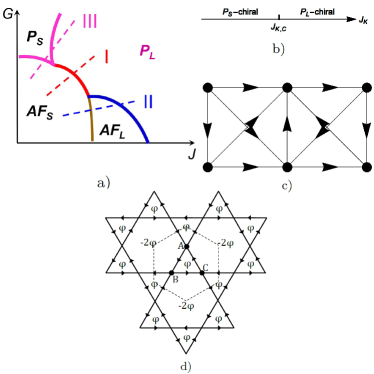
Figure 1: (Color online) (a) The global phase diagram of Kondo lattice systems Si (2010); (b) In highly frustrated regime (large, fixed $G$), $J_{K}$ tunes through a Kondo-destruction QCP (at $J_{K,c}$) from a Kondo-destroyed chiral spin liquid ($P_{S,chiral}$) to a Kondo-screened phase ($P_{L,chiral}$). The $\chi$ fields of the square lattice are shown in the $\pi$-flux state (without the diagonal bonds) and the CSL state (c), and in the CSL state on the Kagomé lattice (d): the arrows denote the sign of gauge field $A_{ij}$, and $\phi$ is the flux through a triangle.

By minimizing the total energy of $H_{eff}$ in Eq. (2), we obtain the phase diagrams containing the chiral states, in which $J_{K}$ tunes the system from the $P_{S}$ to $P_{L}$ phases (see Supplemental Material supp ). Across a second-order Kondo-destroyed $P_{S,chiral}$ to $P_{L,chiral}$ quantum phase transition, Fig. (1b), we consider a power-law form for the Kondo hybridization amplitude:

$$\rho_{K}(J_{K})=\rho_{r}\Big{(}\frac{J_{K}-J_{K,c}}{J_{K}}\Big{)}^{1/2}\quad,$$ (3)

for $J_{K}>J_{K,c}$ and $\rho_{K}=0$, for $J_{K}<J_{K,c}$. We take $J_{K,c}$ as the value where the $P_{L,chiral}$ state becomes energetically competitive and $\rho_{r}$ to be the saturation value of $\rho_{K}$; both values are adopted from the self-consistent calculation for a given set of $(n_{d},J_{1})$  supp .

Mechanism of the AHE - the Kondo destroyed $P_{S}$ phase.  In the Kondo-destroyed $P_{S}$ phase, the static hybridization amplitude vanishes, $\mbox{$\langle\rho_{K,i}\rangle$}=0$. However, we show that there are TRSB terms in the effective interactions among the conduction electrons, which are mediated by the spinons via Kondo couplings. Such terms yield a zero-field AHE.

We will single out the TRSB terms. The TRSB order parameter of the CSL is the spin chirality,

$$\hat{E}_{ijk}=\bm{S}_{i}\cdot(\bm{S}_{j}\times\bm{S}_{k})\quad,$$ (4)

where the indices $\{i,j,k\}$ mark the three sites of an elementary triangle of the lattice. In the CSL state, $E_{ijk}=\mbox{$\langle\hat{E}_{ijk}\rangle$}=2i(P_{ijk}-P_{ikj})$, where $P_{ijk}=\chi_{ij}\chi_{jk}\chi_{ki}$. On symmetry grounds, we expect $E_{ijk}$ to be coupled to the composite chiral operator of the conduction electrons, $\bm{s}_{i}\cdot(\bm{s}_{j}\times\bm{s}_{k})$. With this guidance, we obtain the coupling from integrating out the $f$-fermions and expanding in powers of $J_{K}$; this can be represented by triangular diagrams (Supplemental Material supp ), similar to what is used in deriving a chiral current. We find

$$\begin{split}&H_{\text{chiral}}=\sum\frac{J_{K}^{3}}{3!}\underbrace{(\bm{s}_{i}\cdot\bm{S}_{i})(\bm{s}_{j}\cdot\bm{S}_{j})(\bm{s}_{k}\cdot\bm{S}_{k})}_{\triangle\text{-loop contraction}}\\ &=\frac{J_{K}^{3}}{2\times 3!}E_{ijk}\bm{s}_{i}\cdot(\bm{s}_{j}\times\bm{s}_{k})\quad.\end{split}$$ (5)

In the Kagomé case, the hexagons can also possess non-trivial fluxes. We can, however, restrict to the lowest order in $J_{K}$ in the effective TRSB coupling for the conduction electrons, which corresponds to considering only the fluxes of the triangles.

The chiral interactions appearing in $H_{\text{chiral}}$ have a six-fermion form. We can decouple it by introducing a novel HS transformation that involves triangular diagrams, as described in the Supplemental Materialsupp . We end up with an effective bilinear theory:

$$H_{d}=H_{d,0}+H_{d,1}$$ (6)

with

$$H_{d,1}=\sum_{ij}(g\phi_{j}^{*}\phi_{i}d^{\dagger}_{i}d_{j}+\phi^{*}_{i}G^{-1}_{\phi,ij}\phi_{j}+h.c.)\quad.$$ (7)

Hence, the $\phi$-fields are constrained by the condition that, if they are integrated out, we obtain the same chiral interaction terms at $\mathcal{O}(g^{3})$ by computing the same triangle diagrams. We then replace $\phi_{j}^{*}\phi_{i}$ by its expectation value $G_{\phi,ij}$ and arrive at

$$H_{d,1}\rightarrow\sum_{ij}(gG_{\phi,ij}d^{\dagger}_{i}d_{j}+h.c.)\quad.$$ (8)

It turns out that $G_{\phi,ij}=e^{-iA_{ij}}$, and $g$ can be identified as $g=J_{K}(\lvert E_{ijk}\rvert/2)^{1/3}$. Because the bosonic Gaussian integral has a minus sign relative to its fermionic counterpart, $G_{\phi,ij}$ carries the opposite flux pattern in order to produce the same $H_{\text{chiral}}$ when we integrate out the $\phi$-fields. Physically, the flux (or chirality) pattern has the opposite sign to that of the CSL state, so that the antiferromagnetic Kondo coupling will lower the ground state energy. This effective Hamiltonian is adequate for qualitatively describing the AHE physics of our original Hamiltonian. Other non-chiral effective interactions would only renormalize the Fermi liquid parameters of the $d$-electrons for the $P_{S}$ phase. We can then use the Streda formula Streda (1982); Nagaosa et al. (2010) to compute the AHE coefficient $\sigma_{xy}$: The involved quantities are the current operator of the conduction electrons $v_{a}({\bf k})=\partial_{a}H_{d}({\bf k})$, the Berry curvature $\mathcal{F}^{xy}_{n}({\bf k})$, and the Fermi function $f(\epsilon_{n}({\bf k}))$ (Supplemental Materialsupp ).

Mechanism of the AHE - the Kondo screened $P_{L}$ phase.  In the $P_{L}$ phase, the Kondo order parameter $\rho_{K,i}$ acquires a non-zero expectation value $\rho_{K}=\mbox{$\langle\rho_{K,i}\rangle$}$. There should still be an incoherent piece of the slave boson fields: $\rho_{K,i}=\rho_{K}+\pi^{\prime}_{i}$. Moreover, we focus on the case where the chiral order survives in the $P_{L}$ phase. By considering the same triangular diagrams now mediated by the incoherent part $\pi^{\prime}_{i}$, the fluctuations of the Kondo order parameter still mediate chiral interactions similarly as in the $P_{S}$ phase, but with a reduced weight. However, there is no spectral sum rule for the $\pi^{\prime}_{i}$s to readily obtain this reduced weight. In the Supplemental Material supp , we use a slave rotor approach for the periodic Anderson model to determine this factor. The effective Hamiltonian of the $d$-electrons becomes

$$H_{d}=H_{d,0}+[1-(4J_{K}/U)\rho_{K}^{2}]H_{d,1}\quad,$$ (9)

where $U$ is the onsite Hubbard repulsion. We fix $U=2W$, i.e. twice the $d$-electron’s bandwidth throughout the calculations. Keeping only the $\rho_{K}$ part of $H_{K}$ leads to the following effective Hamiltonian:

$$H_{P_{L}}=\Psi^{\dagger}\begin{pmatrix}H_{\text{CSL}}&-J_{K}\rho_{K}\mathcal{I}\\ -J_{K}\rho_{K}\mathcal{I}&H_{d}\end{pmatrix}\Psi\quad,$$ (10)

where $\mathcal{I}$ is an identity matrix, and $\Psi^{\dagger}=(f^{\dagger},d^{\dagger}).$ We have dropped the spin index, as there are no longer the spin-flip terms. The Hamiltonian $H_{P_{L}}$ is smoothly connected with $H_{d}$ at the QCP. We then compute $\sigma_{xy}$ from the Streda formula Eq. S-22, noting that the current operators remains the same, i.e.  $v_{a}({\bf k})=\partial_{a}H_{d}({\bf k})$.

AHE and its evolution across the Kondo-destruction QCP.  For the square lattice, we focus on the $\pi$-flux and the CSL states. For the $\pi$-flux phase, $H_{QSL}=H_{\pi-flux}$ is given by $A_{\bm{r}_{i},\bm{r}_{i}+\hat{x}}=\pi/2$, $A_{\bm{r}_{i},\bm{r}_{i}+\hat{y}}=-(-1)^{x_{i}}\pi/2$, $\rho_{\bm{r}_{i},\bm{r}_{i}+\hat{x}+\hat{y}}=0$, where $\bm{r}_{i}=(x_{i},y_{i})$, $\hat{x}$ ($\hat{y}$) is the unit vector along the $x(y)$-axis. For the CSL Hamiltonian, $H_{QSL}=H_{CSL}$ is derived from $H_{\pi-flux}$ with $\rho_{\bm{r}_{i},\bm{r}_{i}+\hat{x}+\hat{y}}\neq 0$, $A_{\bm{r}_{i},\bm{r}_{i}+\hat{x}+\hat{y}}=A_{\bm{r}_{i}+\hat{y},\bm{r}_{i}+\hat{x}}=(-1)^{x_{i}}\pi/2$, as illustrated in Fig. (1c).

In the Kagomé lattice, any state with triangle flux $\phi\neq 0,\pi$ breaks TRS. Here, we choose $\phi=-\frac{\pi}{2}$ such that the hexagon flux of $-2\phi=\pi$ preserves TRS. The $(-\frac{\pi}{2},\pi)$ spinon flux state has three well-separated bands; the middle flat band is exactly at the Fermi energy, and the Chern numbers are $C_{lower}=-1$, $C_{middle}=0$, $C_{upper}=+1$ Nagaosa et al. (2010). The phase structure of the corresponding $\chi_{ij}$ fields is plotted in Fig. (1d).

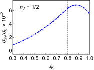
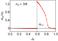
Figure 2: (Color online) Zero field anomalous Hall conductance ($\sigma_{xy}$), normalized by the quantum conductance $\sigma_{0}=e^{2}/h$, for $J_{1}=t=1,\ J_{2}/J_{1}=1/2,\ n_{d}=0.5$ on a square lattice (a) and for $J=t,\ n_{d}=3/8$ on a Kagomé lattice (b).

The zero-field anomalous Hall conductivity $\sigma_{xy}$ of the $J_{1}-J_{2}-J_{K}$ model is shown in Fig. (2) for a representative parameters $n_{d}=0.5,\ J_{1}=t$ and that of the Kagomé lattice model in Fig (2) for $J=t,\ n_{d}=3/8$. Across the QCP, $\sigma_{xy}$ is found continuous in the former, but jumps in the latter.

In order to understand the different behaviors, we show the Fermi surfaces (dashed lines) and the difference of band-summed Berry curvature $\Delta\Omega({\bf k})$ (color map) between the $P_{S}$ phase and the $P_{L}$ phase right across the QCP in Fig. (3) for the square lattice and (3) for the Kagomé lattice (the actual $\Omega({\bf k})$ is shown in Supplemental Material). Here $\Delta\Omega({\bf k})=\Omega_{P_{S}}({\bf k})-\Omega_{P_{L}}({\bf k})$ and $\Omega({\bf k})=\sum_{n}\mathcal{F}^{xy}_{n}({\bf k})f(\epsilon_{n}({\bf k}))$. We find the Fermi surfaces remain continuous for the square lattice model. Both Fermi surfaces of the $P_{S}$ and $P_{L}$ phases are the black dashed line. However, for the Kagomé case, the Fermi surfaces show a jump. The Fermi surface of the $P_{S}$ phase is the black dashed circle in the middle of the BZ which overlaps with the red, singular part of $\Delta\Omega({\bf k})$. Those of the $P_{L}$ phase are the blue dashed-line pockets at the edge of the BZ. These results reflect the number of sites per unit cell as well as the gapped/gapless nature of the spinon spectrum. However, $\Delta\Omega({\bf k})$ is singular and concentrates near Fermi surfaces in both cases. This is because the onset of Kondo hybridization, which acts as a topological mass term in the large-$N$ theory, generally reconstructs the wavefunctions in a singular fashion regardless of whether the Fermi surfaces jump or not.

To reconcile the notions of the singular wavefunction (or Berry curvature) with the continuous AHE, we note that $\sigma_{xy}$ is intrinsically a Fermi surface property Haldane (2004) (apart from the contributions of fully occupied bands). We can analytically show the following by computing the diagonal Berry’s connection in the $\rho_{K}\rightarrow 0$ limit supp . When the Fermi surface is continuous, $\sigma_{xy}$ must be continuous; here, the projected wavefunctions of the $d$-electron are continuous, and so are the Berry connections. By contrast, when the Fermi surface jumps, the projected wavefunctions completely reconstruct due to the existence of two non-commuting topological “masses”: the Kondo screening and a non-zero jump of the spinon Lagrangian multiplier $\lambda$.

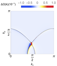
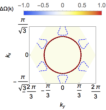
Figure 3: (Color online) Fermi surfaces (dashed curves) and the difference in the band-summed Berry curvature distribution $\Delta\Omega({\bf k})$ between the $P_{S}$ phase and the $P_{L}$ phase (color map) of the square lattice model (3) and the Kagomé lattice model (3).

Discussion. Energetic considerations show that the Kondo coupling favors gapless states (Supplemental Material supp ). For the pyrochlore lattice, the CSL state in the large-$N$ limit is gapless Burnell et al. (2008), and is thus expected to have a similar sequence of quantum phase transitions involving the chiral state. The gapless nature raises the prospect of a sudden reconstruction of the Fermi surface across a Kondo-destruction QCP in the pyrochlore case and, by extension, a jump in the zero-field AHE, especially for a magnetic field along the [111] direction.

We expect the jump of the zero field AHE, $\sigma_{xy}$, to be robust against weak disorder. The AHE effect considered here is intrinsic, i.e. determined by the quasi-particle band structure. Scattering from weak non-magnetic impurities only yields a small (linear in disorder) correction  Sinitsyn2007 . Moreover, the Fermi-surface jump across a Kondo-destruction QCP has been evidenced to be robust against weak disorder Gegenwart et al. (2008); Si and Paschen (2013). Thus, our results can be tested in Pr₂Ir₂O₇, once a control parameter is identified to tune across the implicated zero-field QCP  Tokiwa et al. (2014).

We note that the anomalous Hall conductance from the mechanism advanced here is quite large. Experiments in Pr₂Ir₂O₇ Machida et al. (2010) find a large sheet $\sigma_{xy}$ reaching about 0.7% of $\sigma_{0}\equiv{\rm e}^{2}/h$, a value which readily arise in our mechanism (Fig. 2).

We have emphasized the role of the Kondo effect and its critical destruction. Future work should incorporate ab initio features, not only on the directional dependence in the pyrochlore lattice but also the effect of the ab initio electronic band structure and the non-Kramers nature of the ground-state crystal-field level of the Pr ions Chandra et al. (2013); Rau and Kee (2014). However, we have derived our conclusions in geometrically frustrated Kondo systems and demonstrated the robustness of our results by connecting them with the evolution of the Fermi surfaces. Thus, we expect our results to remain qualitatively valid in the more realistic settings. For Pr₂Ir₂O₇, this is so given the substantial evidence for the role of the Kondo coupling such as the large entropy observed in the pertinent low-temperature regime Tokiwa et al. (2014). It may also be instructive to explore related effects in other $f$-electron systems with geometrical frustration, such as UCu₅ under ambient conditionsUeland et al. (2012) and when suitably tuned through a QCP.

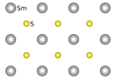
Figure 4: Lattice plane of $g$-SmS.

We close by proposing an engineered Kondo-insulator interface as a model material for the frustrated Kondo lattice Hamiltonian. The motivation for the proposed setting comes from recent advances in the molecular beam epitaxy (MBE) of Kondo systems Shishido et al. (2010); Goh et al. (2012). As a promising candidate material we suggest the golden phase of SmS ($g$-SmS). In bulk samples this phase is stable under pressures between about 0.65 GPa Maple and Wohlleben (1971) and 2 GPa Haga et al. (2004). As MBE thin-film the phase might be stabilized by lattice mismatch with an appropriate substrate. $g$-SmS crystallizes in a face-centered-cubic (fcc) structure of rock-salt (NaCl) type. A lattice plane is shown in Fig. (4). $g$-SmS shows characteristics of a Kondo insulating state in transport Wac94.1 ; Haga et al. (2004), thermodynamics Matsubayashi et al. (2007), and point contact spectroscopy Wac94.1 . From thermal expansion and heat capacity measurements the energy gap was estimated to be 90 K on the low-pressure side of the $g$-SmS phase Matsubayashi et al. (2007). At temperatures low compared to this scale, the proposed lattice plane could then serve as a setting to realize the frustrated $J_{1}-J_{2}$ Kondo lattice and study the anomalous Hall effect.

We would like to acknowledge useful discussions with P. Gegenwart, S. Nakatsuji and P. Goswami. This work was supported in part by the U.S. Army Research Office Grant No. W911NF-14-1-0525 (W.D. and S.E.G.), the U.S. Army Research Office Grant No. W911NF-14-1-0497 (S.P.), the NSF Grant No. DMR-1611392 (for travel support) and the Robert A. Welch Foundation Grant No. C-1411(S.E.G. and Q.S.).

$\dagger$ These two authors contributed equally to this work.

Supplemental Material

.1 Chiral interaction from perturbative expansion

To obtain Eq. (5) of the main text, we integrate out the $f$-spinons from Eqs. (1,2) of the main text in the Kondo destroyed phase using the standard Feynman diagram procedure. Guided by the symmetry analysis, we only need to consider the third-order term $1/3!(\bm{s}_{i}\cdot\bm{S}_{i})(\bm{s}_{j}\cdot\bm{S}_{j})(\bm{s}_{k}\cdot\bm{S}_{k})$. The effective chiral electronic interaction $H_{cc}$ is obtained by contracting the spinons in triangle-loop diagrams as shown Fig. (S1).

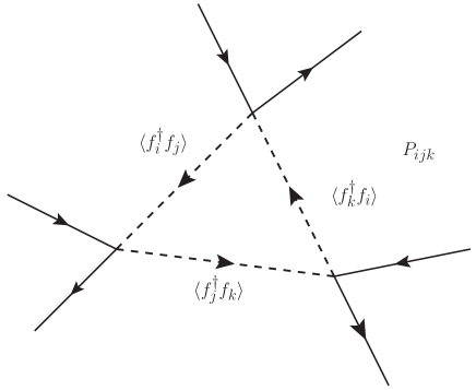
Figure S1: Feynman diagrams of the triangle-loop contractions. The solid lines are the propagators for the conduction electrons.

Since the CSL is gapped, it is sufficient to restrict to the most local three-site loops, i.e. the triangle within a unit cell, at equal time only. Then we can obtain $H_{\text{chiral}}$ as follows:

$$\begin{split}&(\bm{s}_{i}\cdot\bm{S}_{i})(\bm{s}_{j}\cdot\bm{S}_{j})(\bm{s}_{k}\cdot\bm{S}_{k})=\sum_{a,b,c}s_{i}^{a}s_{j}^{b}s_{k}^{c}\\ &\times\frac{1}{8}(f^{\dagger}_{i\alpha_{i}}\sigma^{a}_{\alpha_{i}\beta_{i}}f_{i\beta_{i}}f^{\dagger}_{j\alpha_{j}}\sigma^{b}_{\alpha_{j}\beta_{j}}f_{j\beta_{j}}f^{\dagger}_{k\alpha_{k}}\sigma^{c}_{\alpha_{k}\beta_{k}}f_{k\beta_{k}})\\ &\underrightarrow{\triangle}\sum_{a,b,c}s_{i}^{a}s_{j}^{b}s_{k}^{c}(\mbox{$\langle f^{\dagger}_{i\alpha_{i}}f_{j\beta_{j}}\rangle$}\mbox{$\langle f^{\dagger}_{j\alpha_{j}}f_{k\beta_{k}}\rangle$}\mbox{$\langle f^{\dagger}_{k\alpha_{k}}f_{i\beta_{i}}\rangle$}\\ &+\mbox{$\langle f^{\dagger}_{i\alpha_{i}}f_{k\beta_{k}}\rangle$}\mbox{$\langle f^{\dagger}_{k\alpha_{k}}f_{j\beta_{j}}\rangle$}\mbox{$\langle f^{\dagger}_{j\alpha_{j}}f_{i\beta_{i}}\rangle$})\sigma^{a}_{\alpha_{i}\beta_{i}}\sigma^{b}_{\alpha_{j}\beta_{j}}\sigma^{c}_{\alpha_{k}\beta_{k}}\\ &=E_{ijk}\bm{s}_{i}\cdot(\bm{s}_{j}\times\bm{s}_{k})/2,\end{split}$$ (S-1)

where $\underrightarrow{\triangle}$ denotes triangular-loop contraction. The constraction is approximated by equal-time correlators, so $\mbox{$\langle f^{\dagger}_{i\alpha_{i}}f_{j\beta_{j}}\rangle$}=\delta_{\alpha_{i},\beta_{j}}\chi_{ij}$. Discarding the density-density interactions, the second line of Eq. (S-1) can be written as

$$\begin{split}&H_{\text{chiral}}\sim\sum_{\alpha_{l},\alpha_{j},\alpha_{k}}(P_{ljk}d^{\dagger}_{l\alpha_{k}}d_{l\alpha_{l}}d^{\dagger}_{j\alpha_{l}}d_{j\alpha_{j}}d^{\dagger}_{k\alpha_{j}}d_{k\alpha_{k}}\\ &+P_{lkj}d^{\dagger}_{l\alpha_{j}}d_{l\alpha_{l}}d^{\dagger}_{k\alpha_{l}}d_{k\alpha_{k}}d^{\dagger}_{j\alpha_{k}}d_{j\alpha_{j}}).\end{split}$$ (S-2)

$H_{\text{chiral}}$ of the Kondo Screened Phase. In order to obtain the spectral weight of the incoherent terms in the Kondo screened phase, we use the slave rotor theoryFlorens and Georges (2004) to tackle the $f$-fermion Hubbard model. As we shall briefly discuss below, the Kondo transition is the Mott transition for $f$-fermions in perdiodic Anderson model (PAM)Florens and Georges (2002), and is realized when the rotor fields are condensed. The condensation density describes the coherent charge degrees of freedom that would contribute to transport.

The PAM Hamiltonian is

$$H_{\text{PAM}}=H^{(f^{\prime})}_{\text{Hubbard}}+H_{0}^{(d)}+V\sum_{i,\sigma}(f^{\prime\dagger}_{i,\sigma}d_{i,\sigma}+f^{\prime}_{i,\sigma}d^{\dagger}_{i,\sigma}),$$ (S-3)

where

$$H^{(f^{\prime})}_{\text{Hubbard}}=-\sum_{ij,\sigma}t_{ij}f^{\prime\dagger}_{i,\sigma}f^{\prime}_{j,\sigma}+U\sum_{i,\sigma,\sigma^{\prime}}n^{(f^{\prime})}_{i,\sigma}n^{(f^{\prime})}_{i,\sigma^{\prime}}$$ (S-4)

is the usual half-filled Hubbard model, and

$$H_{0}^{(d)}=-\sum_{ij,\sigma}t_{ij}d^{\dagger}_{i,\sigma}d_{j,\sigma}$$ (S-5)

describes the free $d$-band electrons.

First, we use the slave rotor formalism to treat the Hubbard model part by letting $f^{\prime}_{i}\rightarrow f_{i}e^{-i\theta_{i}}$

$$H^{(f^{\prime})}\rightarrow\frac{U}{2}\sum_{i,\sigma}\hat{L}_{i,\sigma}^{2}-\sum_{ij,\sigma}(t_{ij}f^{\dagger}_{i,\sigma}f_{j,\sigma}e^{i(\theta_{i}-\theta_{j})}+h.c.).$$ (S-6)

The corresponding Lagrangian is

$$\begin{split}&S_{H}=\int d\tau\sum_{i,\sigma}f^{\dagger}_{i,\sigma}\partial_{\tau}f_{i,\sigma}+\frac{(\partial_{\tau}\theta)^{2}}{2U}+\\ &\sum_{\mbox{$\langle ij\rangle$},\sigma}(t_{\mbox{$\langle ij\rangle$}}f^{\dagger}_{i,\sigma}f_{j,\sigma}e^{i(\theta_{i}-\theta_{j})}+h.c.),\end{split}$$ (S-7)

here the kinetic energy of the rotors $\frac{U}{2}\sum_{i,\sigma}\hat{L}_{i,\sigma}^{2}$ is replaced by its conjugate variables $\hat{L}_{i,\sigma}=(\partial_{\tau}\theta+ih)/U$.

Let $e^{i\theta_{i}}=X_{i}$, so that $X_{i}$s subject to the constraint $\lvert X_{i}\rvert^{2}=1$ on average (using Lagrangian multiplier). Using $\partial_{\tau}\theta_{i}=\frac{1}{i}X_{i}^{*}\partial_{\tau}X_{i}$, we have

$$S_{H}=S^{0}_{X}+S_{f}^{0}+\sum_{\mbox{$\langle ij\rangle$},\sigma}(t_{\mbox{$\langle ij\rangle$}}f^{\dagger}_{i,\sigma}f_{j,\sigma}X_{i}X^{*}_{j}+h.c.).$$ (S-8)

with $S^{0}_{f}=\int d\tau\sum_{i,\sigma}f^{\dagger}_{i,\sigma}\partial_{\tau}f_{i,\sigma}$, and $S_{X}^{0}=\sum_{i}(\frac{\lvert\partial_{\tau}X_{i}\rvert^{2}}{2U}+\lambda_{i}(\lvert X_{i}\rvert^{2}-1))$. The exchange term is also expressed in terms of slave rotors

$$H_{\text{exc}}=V\sum_{i,\sigma}(f^{\dagger}_{i,\sigma}d_{i,\sigma}X_{i}+h.c.).$$ (S-9)

In the large-$U$-small-$V$ limit, the system is in $P_{S}$ phase. We can integrate out the rotor fields, and recover both the Heisenberg-$J$ interaction, as well as the Kondo coupling

$$H_{K}=J_{K}\sum_{i}\bm{S}_{f}(i)\cdot\bm{s}_{d}(i),$$ (S-10)

where $J_{K}=4V^{2}/U$.

Within the slave rotor approach, the onset of Kondo screening is described by the condensation of the $X$-field: $X_{i}\rightarrow X^{0}_{i}+X^{\prime}_{i}$. The exchange term becomes

$$H_{exc}=\sum_{i,\sigma}(VX^{0}_{i}f^{\dagger}_{i,\sigma}d_{i,\sigma}+VX^{\prime}_{i}f^{\dagger}_{i,\sigma}d_{i,\sigma}+h.c.).$$ (S-11)

The first term is the hybridazation term, which is equivalent to that of the Kondo model. We can identify that $\rho_{K}=VX^{0}_{i}/J_{K}=\frac{U}{4V}X^{0}_{i}$. The second term now provides the incoherent fluctuations, which, as we argue in the main text, can mediate the same chiral interactions for the $d$-electrons through the triangular diagrams. But in this approach, the $X$-field satisfies a spectral sum rule: $\int d\nu d^{2}k/(2\pi)^{3}G_{X}(\nu;{\bf k})=1$, from which we can obtain that in the Kondo screened phase

$$H_{\text{chiral}}=\left(1-\frac{4J_{K}}{U}\rho_{K}^{2}\right)^{3}\frac{J_{K}^{3}}{2}E_{ijk}\bm{s}_{i}\cdot(\bm{s}_{j}\times\bm{s}_{k}).$$ (S-12)

Note that the prefactor $4J_{K}/U$ is changing as we tune $J_{K}$. In our calculation, we fix $U=16t$, i.e. twice as the $d$-electron’s bandwidth.

Hubbard-Stratonovich transformation of $H_{\text{chiral}}$. To decouple the six-fermion chiral interaction, in general we need to introduce two sets of Hubbard-Stratonovich (HS) fields, namely, $\gamma$s, $\kappa$s, which can be interpreted as a single bond / two consecutive bonds fields:

$$\gamma_{ij} =\mbox{$\langle\sum_{\alpha}d^{\dagger}_{i,\alpha}d_{j,\alpha}\rangle$},$$ (S-13)

$$\kappa_{ij,k} =\mbox{$\langle\sum_{\alpha,\beta}d^{\dagger}_{i,\alpha}d_{k,\alpha}d^{\dagger}_{k,\beta}d_{j,\beta}\rangle$},$$ (S-14)

which are in principle independent. The bond indices here are directional, i.e. $\gamma_{ji}=\gamma_{ij}^{*}$, $\kappa_{ji,k}=\kappa_{ij,k}^{*}$. In general, we have 6 complex $\gamma$’s and 12 complex $\kappa$’s.

The HS transformation is as follows

$$L_{\text{HS}}=\sum_{\bm{x}}(d^{\dagger}_{\bm{x}}(i\partial_{t}+\mu)d_{\bm{x}}-\widetilde{\Psi}^{*}\mathcal{M}\Psi+J^{\dagger}\Psi+\widetilde{\Psi}^{*}J-H_{\text{kin}}),$$ (S-15)

where $\widetilde{\Psi}^{*}=\{\kappa^{*}_{\bm{x}_{i}\bm{x}_{j},k},\dots\kappa^{*}_{\bm{x}_{i}\bm{x}_{j},\bar{k}},\dots,\gamma^{*}_{\bm{x}_{i}\bm{x}_{j}},\dots,\gamma_{\bm{x}_{j}\bm{x}_{i}}^{*},\dots\}$ is a 24-component vector. The indices $i-j$ run over all the links inside a unit cell given by $\bm{x}$, and $\{k,\bar{k}\}$ denote the other two sites for a given bond $\langle ij\rangle$ within the unit cell.

$$\begin{split}&J^{\dagger}=\{\hat{\gamma}^{\dagger}_{ij},\hat{\gamma_{ji}}^{\dagger},\dots,{\kappa}_{ij,k}^{\dagger},\hat{\kappa}_{ij,\bar{k}}^{\dagger},\dots\}.\end{split}$$ (S-16)

where we use $\hat{\gamma}_{ij}^{\dagger}=\sum_{\alpha}d^{\dagger}_{\bm{x}_{j},\alpha}d_{\bm{x}_{i},\alpha}$, $\hat{\kappa}^{\dagger}_{ij,k}=\sum_{\alpha,\beta}d^{\dagger}_{j,\alpha}d_{k,\alpha}d^{\dagger}_{k,\beta}d_{i,\beta}$.

To determine $\mathcal{M}$, suppose that we now integrate out all the HS fields, we should recover the effective interactions as

$$H_{eff-int}=J^{\dagger}\mathcal{M}^{-1}J=H_{\text{cc}}+\dots,$$ (S-17)

in which the $\dots$ indicates other effective interactions. To have a stable HS transformation, we need to further include the 4-fermion effective interactions at $H^{(2)}_{eff-int}\sim\mathcal{O}(J_{K}^{2})$ generated from $J_{K}^{2}(\bm{s}_{i}\cdot\bm{S}_{i})(\bm{s}_{j}\cdot\bm{S}_{j})$ as well as the 8-fermion process at $H^{(4)}_{eff-int}\sim\mathcal{O}(J_{K}^{4})$. Since the $f$-fermions are gapped, we can keep only the short-range terms, i.e. within a unit cell, so that all the terms can be decoupled by the $\hat{\gamma}_{ij}$s and $\hat{\kappa}_{ij}$s in the large-$N$ limit. Then $\mathcal{M}^{-1}$ can be written in a block form $\mathcal{M}^{-1}=\oplus(\mathcal{M}^{-1}_{(ij)})$, where $(\mathcal{M}^{-1}_{(ij)})$ is a $4\times 4$ matrix for a given bond $(ij)$ within the unit cell.

Here we estimate the matrix elements of $(\mathcal{M}^{-1}_{(ij)})$ within the approximations that are used for computing $H_{\text{chiral}}$, i.e. equal-time contraction is used and only those within a unit cell are included:

$$(M^{-1})_{\hat{\gamma}^{\dagger}\hat{\gamma},(ij)}=J_{K}^{2}\text{sgn}[(ij)]\chi_{ij}\chi_{ji}/2!=\rho_{ij}^{2},$$ (S-18)

$$(M^{-1})_{\hat{\kappa}\hat{\gamma},(ij)k}=J_{K}^{3}P_{ijk}/(2\times 3!),$$ (S-19)

$$(M^{-1})_{\hat{\kappa}^{\dagger}\hat{\kappa},(ij),kk^{\prime}}=\delta_{k,k^{\prime}}J_{K}^{4}\rho_{ij}^{4}/4!.$$ (S-20)

$\text{sgn}[\mbox{$\langle ij\rangle$}]$ is a relative sign coming from the fact that $\hat{\gamma_{ij}}^{\dagger}\hat{\gamma_{ij}}\sim-\hat{\gamma_{ji}}^{\dagger}\hat{\gamma_{ji}}$. We see that $\det[M^{-1}]$ is indeed positive, and hence this is a stable HS transformation. $\mathcal{M}$ is then obtained by inversing $\mathcal{M}^{-1}$.

Therefore, we have a formal HS decoupling of $H_{\text{chiral}}$. Further replacing the HS-fields by their expectation values in Eq. (S-15), we obtain both fermion bilinears and four-fermion terms. To lower the total energy, we need to have $\gamma_{ij}\kappa^{*}_{ij,k}\sim-P_{ijk}$. Upon satisfying this constraint, we have an additional gauge degree of freedom to choose either $\gamma_{d,ij}$ or $\kappa^{*}_{ij,k}$ to be imaginary, i.e. explicitly breaking TRS, even though the underlying physical state is the same. For convenience, we can choose $\kappa^{*}_{ij,k}$s which couple to $d$-fermion bilinears ($\hat{\gamma}_{ij}$s) to be TRSB. By keeping only the TRSB terms in Eq. (S-15), we justify our choice of Eq. (8) in the main text as

$$H_{d,1}=\sum_{\mbox{$\langle ij\rangle$},k}(\kappa^{*}_{ij,k}\hat{\gamma}_{ij}+h.c.).$$ (S-21)

.2 Berry curvature, Berry connection, Streda formula and Kubo formula

The AHE coefficient, $\sigma_{xy}$, presented in the main text are computed using the Streda formula:

$$\begin{split}\sigma_{xy}&=\int\frac{d{\bf k}}{(2\pi)^{2}}\sum_{n}\mathcal{F}^{xy}_{n}({\bf k})f(\epsilon_{n}({\bf k}))\\ &=\sum_{n\neq n^{\prime}}\int\frac{d{\bf k}}{(2\pi)^{2}}[f(\epsilon_{n}({\bf k}))-f(\epsilon_{n^{\prime}}({\bf k}))]\\ &\times\text{Im}\frac{\mbox{$\langle n,{\bf k}|v_{x}({\bf k})|n^{\prime},{\bf k}\rangle$}\mbox{$\langle n^{\prime},{\bf k}|v_{y}({\bf k})|n,{\bf k}\rangle$}}{[\epsilon_{n}({\bf k})-\epsilon_{n^{\prime}}({\bf k})]^{2}}\quad.\end{split}$$ (S-22)

Here, $v_{a}({\bf k})=\partial_{a}H_{d}({\bf k})$ is the current operator of the conduction electrons, $\mathcal{F}^{xy}_{n}({\bf k})$ the Berry curvature, and $f(\epsilon_{n}({\bf k}))$ the Fermi function. Both $\hbar$ and $e$ have been taken to be $1$.

To discuss the role of the Berry curvature, we start from the more standard Kubo formula. The current operators are

$$\bm{J}_{\bm{q}}=\frac{1}{\sqrt{N}}\sum_{{\bf k}}c^{\dagger}_{{\bf k}+\bm{q}/2}\frac{\partial H_{k}}{\partial{\bf k}}c_{{\bf k}-\bm{q}/2}.$$ (S-23)

In frequency-momentum space, the conductivity is computed via the current-current correlation function

$$\begin{split}&\pi_{ab}(i\nu)=\sum_{\omega}\int\frac{d^{2}k}{(2\pi)^{2}}\text{Tr}\Big{[}\frac{\partial H}{\partial k_{a}}\\ &\times G(\omega-\nu,{\bf k}-\bm{q}/2)\frac{\partial H}{\partial k_{b}}G(\omega,{\bf k}+q/2)\Big{]},\end{split}$$ (S-24)

where the sum over $\omega$ is Matsubara sum.

$$\sigma_{ab}=\lim_{\omega\rightarrow 0}\Big{[}-\text{Im}[\pi_{ab}(i\nu)/\nu\big{|}_{i\nu\rightarrow\omega+i0^{+}}]\Big{]}.$$ (S-25)

For convenience, it is better to write both $G$ and $H$ in terms of the bloch bands projection operators $P_{n}({\bf k})=\mbox{$|n,{\bf k}\rangle\!\langle n,{\bf k}|$}$ (which is possible for fermion bilinear theory) with $|n,{\bf k}\rangle$ being the eigenvectors of $n$th band at momentum ${\bf k}$:

$$H({\bf k}) =\sum_{n}\epsilon_{n}({\bf k})P_{n}({\bf k}),$$ (S-26)

$$G(\omega,{\bf k}) =\sum_{n}\frac{P_{n}({\bf k})}{i\omega-\epsilon_{n}({\bf k})}.$$ (S-27)

After inserting the expression into Eq. (S-24), we find only the following term contributes

$$\begin{split}&\pi_{ab}(i\nu)=\sum_{\omega}\int\frac{d^{2}k}{(2\pi)^{2}}\sum_{n_{0},\dots,n_{3}}\text{Tr}\Big{[}\partial_{k_{a}}P_{n_{0}}\\ &\times P_{n_{1}}\partial_{k_{b}}P_{n_{2}}P_{n_{3}}\frac{\epsilon_{n_{0}}\epsilon_{n_{2}}}{(i(\omega-\nu)-\epsilon_{n_{1}})(i\omega-\epsilon_{n_{3}})}\Big{]}\\ &=\int\frac{d^{2}k}{(2\pi)^{2}}\sum_{n_{0},\dots,n_{3}}\text{Tr}\Big{[}\partial_{k_{a}}P_{n_{0}}\\ &\times P_{n_{1}}\partial_{k_{b}}P_{n_{2}}P_{n_{3}}\frac{\epsilon_{n_{0}}\epsilon_{n_{2}}(f(\epsilon_{n_{3}})-f(\epsilon_{n_{1}}))}{i\nu+\epsilon_{n_{3}}-\epsilon_{n_{1}}}\Big{]}.\end{split}$$ (S-28)

Here $f(\epsilon)$ is the Fermi distribution function, and arises from the Matsubara sum. Sum of $n_{i}$ runs over band indices. After performing the Tr operation, we end up with the following result

$$\begin{split}&\pi_{ab}(i\nu)=\int\frac{d^{2}k}{(2\pi)^{2}}\sum_{n,n^{\prime}}\Big{[}-A_{nn^{\prime}}^{a}A_{n^{\prime}n}^{b}\frac{f(\epsilon_{n})-f(\epsilon_{n^{\prime}})}{i\nu+\epsilon_{n}-\epsilon_{n^{\prime}}}\epsilon_{n}\epsilon_{n^{\prime}}\\ &+A^{a}_{nn^{\prime}}A^{b*}_{n^{\prime}n}\frac{f(\epsilon_{n})-f(\epsilon_{n^{\prime}})}{i\nu+\epsilon_{n}-\epsilon_{n^{\prime}}}\epsilon^{2}_{n^{\prime}}+A^{a*}_{nn^{\prime}}A^{b}_{n^{\prime}n}\frac{f(\epsilon_{n})-f(\epsilon_{n^{\prime}})}{i\nu+\epsilon_{n}-\epsilon_{n^{\prime}}}\epsilon^{2}_{n}\\ &-A_{nn^{\prime}}^{a*}A_{n^{\prime}n}^{b*}\frac{f(\epsilon_{n})-f(\epsilon_{n^{\prime}})}{i\nu+\epsilon_{n}-\epsilon_{n^{\prime}}}\epsilon_{n}\epsilon_{n^{\prime}}\Big{]},\end{split}$$ (S-29)

where $A_{n,n^{\prime}}^{a}=-i\mbox{$\langle n|\partial_{k_{a}}n^{\prime}\rangle$}$, $A_{n,n^{\prime}}^{a*}=-i\mbox{$\langle\partial_{k_{a}}n|n^{\prime}\rangle$}$ is the matrix element of $\partial_{k_{a}}$. Note only the diagonal elements are the Berry connection. Then we do analytic continuation $i\nu\rightarrow\omega+i\eta$, and take the imaginary part of $\pi_{ab}(\omega)/\omega$. In the end, we let $\omega\rightarrow 0$. When we take imaginary part of $\pi_{ab}(\omega)/\omega$, we have two different contributions:

$$\begin{split}&\pi_{ab}^{(1)}=\int\frac{d^{2}k}{(2\pi)^{2}}\sum_{n,n^{\prime}}\Big{(}\text{Im}[-A_{nn^{\prime}}^{a}A_{n^{\prime}n}^{b}]\\ &\times\text{Re}[\frac{f(\epsilon_{n})-f(\epsilon_{n^{\prime}})}{\omega+\epsilon_{n}-\epsilon_{n^{\prime}}+i\eta}\epsilon_{n}\epsilon_{n^{\prime}}]+\dots\Big{)},\end{split}$$ (S-30)

$$\begin{split}&\pi_{ab}^{(2)}=\int\frac{d^{2}k}{(2\pi)^{2}}\sum_{n,n^{\prime}}\Big{(}\text{Re}[-A_{nn^{\prime}}^{a}A_{n^{\prime}n}^{b}]\\ &\times\text{Im}[\frac{f(\epsilon_{n})-f(\epsilon_{n^{\prime}})}{\omega+\epsilon_{n}-\epsilon_{n^{\prime}}+i\eta}\epsilon_{n}\epsilon_{n^{\prime}}]+\dots\Big{)},\end{split}$$ (S-31)

where $\dots$ denotes the rest three terms. Note that $A_{nn^{\prime}}^{a}=-A_{nn^{\prime}}^{a*}$, $(A_{nn^{\prime}}^{a})^{*}=A_{n^{\prime}n}^{a*}$, we find

$$\begin{split}&\pi_{ab}^{(1)}=\int\frac{d^{2}k}{(2\pi)^{2}}\sum_{n,n^{\prime}}\Big{(}\text{Im}[-A_{nn^{\prime}}^{a}A_{n^{\prime}n}^{b}](f(\epsilon_{n})-f(\epsilon_{n^{\prime}}))\\ &\times\text{Re}[\frac{(\epsilon_{n}-\epsilon_{n^{\prime}})^{2}}{\omega+\epsilon_{n}-\epsilon_{n^{\prime}}+i\eta}+\frac{(\epsilon_{n}-\epsilon_{n^{\prime}})^{2}}{\omega-\epsilon_{n}+\epsilon_{n^{\prime}}+i\eta}]\\ &=\int\frac{d^{2}k}{(2\pi)^{2}}\sum_{n,n^{\prime}}\Big{(}\text{Im}[-A_{nn^{\prime}}^{a}A_{n^{\prime}n}^{b}](f(\epsilon_{n})-f(\epsilon_{n^{\prime}}))\\ &\times\frac{2\omega(\epsilon_{n}-\epsilon_{n^{\prime}})^{2}}{\omega^{2}-(\epsilon_{n}-\epsilon_{n^{\prime}})^{2}}.\end{split}$$ (S-32)

Therefore, after taking the limit $\pi_{ab}^{(1)}/\omega|_{\omega\rightarrow 0}$, we obtain

$$\sigma^{(1)}_{ab}=\int\frac{d^{2}k}{(2\pi)^{2}}\sum_{n\neq n^{\prime}}\text{Im}[A_{nn^{\prime}}^{a}A_{n^{\prime}n}^{b}](f(\epsilon_{n})-f(\epsilon_{n^{\prime}})),$$ (S-33)

which we can use the relation $\mbox{$\langle n|\partial_{k_{a}}H(k)|n^{\prime}\rangle$}=(\epsilon_{n}-\epsilon_{n^{\prime}})A_{nn^{\prime}}^{a}+\delta_{n,n^{\prime}}\partial_{k_{a}}\epsilon_{n}$ to transform into the Streda formula. For $\pi_{ab}^{(2)}/\omega|_{\omega\rightarrow 0}$,

$$\text{Im}[\frac{f(\epsilon_{n})-f(\epsilon_{n^{\prime}})}{\omega+\epsilon_{n}-\epsilon_{n^{\prime}}+i\eta}]=\delta_{n,n^{\prime}}\delta(\omega)\frac{f(\epsilon_{n})-f(\epsilon_{n}+\omega)}{\omega}|_{\omega\rightarrow 0}.$$ (S-34)

Note that for $n\neq n^{\prime}$, the factor is immediately zero when we take $\eta\rightarrow 0$. Only $n=n^{\prime}$ terms survive, and $\pi_{ab}^{(2)}/\omega|_{\omega\rightarrow 0}\sim\delta(\omega)\partial f(\epsilon)/\partial\epsilon$. For $a\neq b$, $\text{Re}[A_{nn}^{a}A_{nn}^{b}]$ is symmetric upon exchanging $a\leftrightarrow b$. On the other hand, we know $\pi_{ab}=-\pi_{ba}$. Therefore, $\pi_{ab}^{(2)}=0$ for $a\neq b$. When $a=b$, we recover the usual Kubo formula result of dc conductivity $\sigma_{xx}\sim\delta(\omega)$.

To show that $\sigma_{xy}^{AH}$ is a Fermi surface propertyHaldane (2004), we can rewrite Eq. (S-33) through an integration by part, and make use the fact Sun and Fradkin (2008) that $\sum_{n^{\prime}}\text{Im}[A_{nn^{\prime}}^{a}A_{n^{\prime}n}^{b}]=\nabla_{{\bf k}}^{a}A_{nn}^{b}-\nabla_{{\bf k}}^{b}A_{nn}^{a}$:

$$\begin{split}&\sigma^{(1)}_{ab}=\int\frac{d^{2}k}{2\pi^{2}}\sum_{n}f(\epsilon_{n})(\nabla_{{\bf k}}^{a}A_{nn}^{b}-\nabla_{{\bf k}}^{b}A_{nn}^{a})\\ &=\int\frac{d^{2}k}{2\pi^{2}}\sum_{n}(A_{nn}^{b}\nabla_{{\bf k}}^{a}f(\epsilon_{n})-A_{nn}^{a}\nabla_{{\bf k}}^{b}f(\epsilon_{n}))\\ &=\sum_{n}\frac{1}{2\pi^{2}}\oint A^{a}_{n}({\bf k}_{F})d{\bf k}_{Fa}.\end{split}$$ (S-35)

.3 Berry curvature distribution

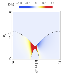
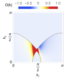
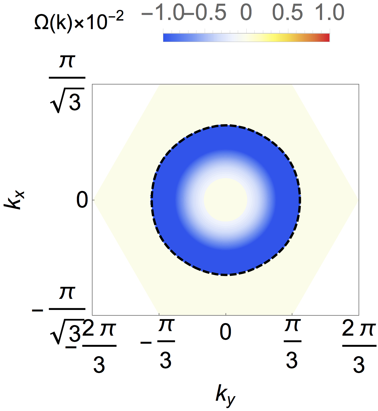
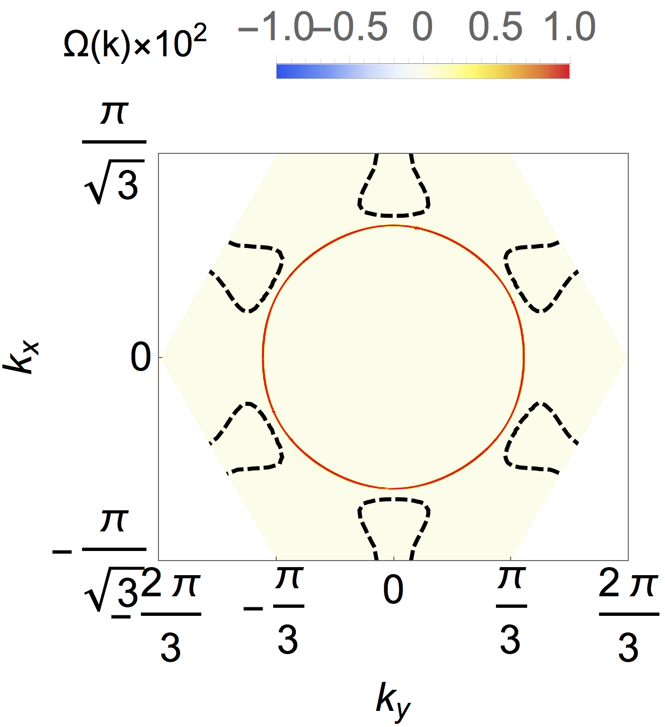
Figure S2: (Color online) The Berry curvature distributions for the square lattice model $P_{S}$ phase (S2), $P_{L}$ phase (S2), the Kagomé lattice model $P_{S}$ phase (S2) and $P_{L}$ phase (S2). The Fermi surfaces are also shown as black dashed lines.

The Berry curvature distributions are shown in Fig. (S2) for $P_{S}$ phase (S2) and $P_{L}$ phase (S2)) the square lattice model, $P_{S}$ phase (S2) and $P_{L}$ phase (S2) of the kagomé lattice model. For (S2) and (S2), despite the visual resemblance, their difference is still significant as shown in Fig. (3a).

.4 Reconstruction of Fermi Surfaces

We note that in the Kondo-destroying $P_{S}$ phase, only conduction electrons participate in forming the Fermi surface. By contrast, in the Kondo-screened $P_{L}$ phase, both the conduction electrons and local $f$-moments are involved in forming the Fermi surface Oshikawa (2000). In the case of the $J_{1}-J_{2}$ model, the spinon excitations of the CSL phase are gapped. By contrast, in the Kagomé case, they are gapless.

To illustrate the point, we show the projected density of states (DOS) in Fig. (S3). The parent spinon TRSB flux state is gapped at zero energy (referred to as “$E_{F}$”) for the $J_{1}-J_{2}$ case, but is gapless at $E_{F}$ for the Kagomé case. The DOS structure of the spinons survives the $P_{L}$ phase (bottom row), but are constrained to straddle $E_{F}$. The Fermi surface is only affected in the Kagomé lattice.

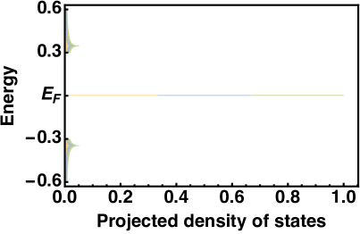
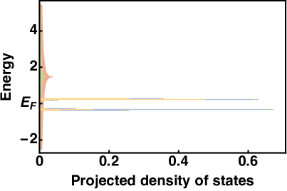
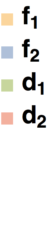
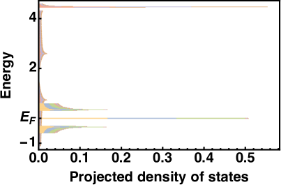
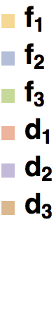
Figure S3: Density of states projected to the sites of a unit cell, for (a) $J_{1}-J_{2}$ spinons in CSL state, (c) kagomé spinons in ($\frac{\pi}{2},-\pi$) state, (e) Kondo screened phase of $J_{1}-J_{2}$ model, (g) Kondo screened phase of Kagomé model; (b),(d),(f),(h) show the relevant legends for color corresponding to the original eigenfunction elements.

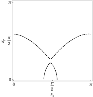
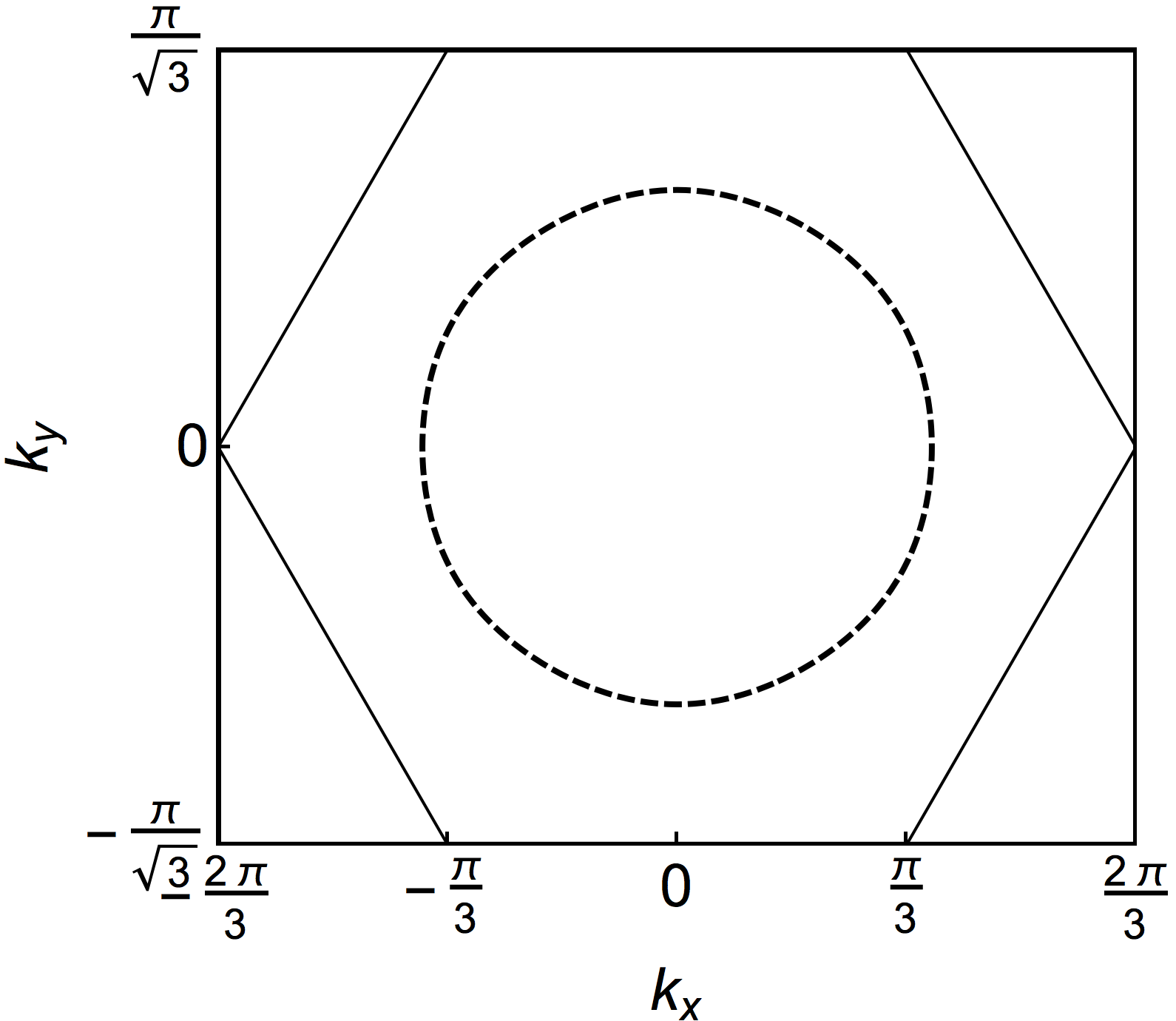
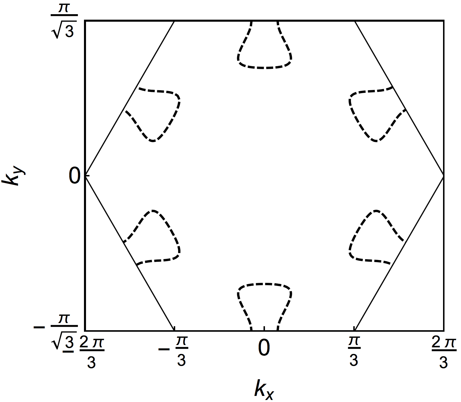
Figure S4: The Fermi surfaces of the square lattice model in the $P_{S}$ phase (S4) and in the $P_{L}$ (S4) phase, and of the Kagomé lattice model in the $P_{S}$ phase (S4) and in the $P_{L}$ phase (S4).

This can be seen by directly plotting the Fermi surfaces. Fig. (S4) shows both the Kondo-destroyed and the Kondo-screened phases, for both the square lattice and the Kagomé lattice. It is clearly seen that, for the $J_{1}-J_{2}$ model on the square lattice, the Fermi surface smoothly evolves through the QCP. By contrast, for the Kagomé lattice, the Fermi surface experiences a sudden jump across the QCP. We also note that the jump is very substantial. This is because, in the Kagomé CSL state, the middle spinon band happens to be a flat band.

.5 Analysis of the wavefunction reconstruction across the QCP

To further our understanding about the nonanalyticities across the QCP, we rewrite the Hamiltonian across the QCP in terms of the $d$-band and $f$-band eigenstates, which we denote as $|\phi^{d}_{\bm{k}}\rangle$ and $|\phi^{f}_{\bm{k}}\rangle$ respectively:

$$\begin{split}&H=\\ &\sum_{\bm{k}}\begin{pmatrix}(\epsilon^{d}_{\bm{k}}-\mu+\lambda^{\prime})\mbox{$|\phi^{d}_{\bm{k}}\rangle$}\mbox{$\langle\phi^{d}_{\bm{k}}|$}&\delta\mbox{$|\phi^{d}_{\bm{k}}\rangle$}\mbox{$\langle\phi^{f}_{\bm{k}}|$}\\ \delta\mbox{$|\phi^{f}_{\bm{k}}\rangle$}\mbox{$\langle\phi^{d}_{\bm{k}}|$}&(\epsilon^{f}_{\bm{k}}-\mu-\lambda^{\prime})\mbox{$|\phi^{f}_{\bm{k}}\rangle$}\mbox{$\langle\phi^{f}_{\bm{k}}|$}\end{pmatrix}.\end{split}$$ (S-36)

Here, $\delta$ is the hybridization strength. In addition, $\lambda^{\prime}$ is the Lagrangian multiplier, which is shifted from $\lambda$ by a constant that can be absorbed into $\mu$, to obtain the above symmetric form for later convenience. The hybridization, thus the wavefunction reconstruction, is the strongest at the $\bm{k}$ points where the conduction bands and spinon bands intersect, i.e. $\epsilon^{f}_{\bm{k}_{0}}-\mu=\epsilon^{d}_{\bm{k}_{0}}-\mu=0$.

For the Kagomé case, Consider the case that the Fermi surface jumps. We expect $\lambda^{\prime}$ to track $\delta$ as the QCP is approached. Nonetheless, we can still start out with the points where $\epsilon^{f}_{\bm{k}_{0}}-\mu=\epsilon^{d}_{\bm{k}_{0}}-\mu=0$. In this case, we can write the $\lambda^{\prime}$ term as $\lambda^{\prime}\sigma_{0}\otimes\tau_{z}$, where $\tau_{z}$ is the Pauli matrix for the orbital space. This term does not commute with the hybridization term, which is off-diagonal in the $\tau$ space. (Note that both the diagonal and off-diagonal blocks above are diagonal matrices in the sublattice space, and therefore commute with each other in that space.) Therefore, the presence of any $\lambda^{\prime}$ prevents us from block-diagonalizing the Hamiltonian even for infinitesimal $\delta$. The new eigenstates are therefore reconstructed completely.

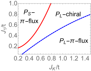
Figure S5: (Color online) The phase diagram of $J_{1}-J_{2}-J_{K}$ model with $J_{2}=J_{1}/2$ and $n_{d}=0.5$ (S5).

.6 Phase diagram in the saddle-point analysis

To illustrate our procedure, we consider the phase diagram arising from the saddle-point analysis in the case of $J_{1}-J_{2}$ square lattice. We minimize the total energy of Eq. (2) with respect to the amplitudes of the link fields $\rho_{ij}$ and $\rho_{K,i}$. The phase diagram of the square lattice model is shown in Fig. (S5), where the red (solid) and blue (dashed) lines respectively mark a first-order phase transition and a crossover. It shows that both the flux-state and the chiral-state solutions can be stabilized, i.e. having lower energies than the unhybridized phase, for $J_{K}$ larger than some critical $J_{K,c}$. The flux phase solution has the lowest energy when stabilized, signaling that the Kondo coupling favors the gapless states.

For the pyrochlore lattice, the CSL state is gapless Burnell2009s , and our result here strongly suggests that a similar chiral state could be the ground state on the pyrochlore lattice when the Kondo coupling is introduced.