Extremals in the Engel group with a sub-Lorentzian metric

Abstract:

Let $E$ be the Engel group and $D$ be a rank 2 bracket generating left invariant distribution with a Lorentzian metric, which is a nondegenerate metric of index 1. In this paper, we first prove that timelike normal extremals are locally maximizing. Second, we obtain a parametrization of timelike, spacelike, lightlike normal extremal trajectories by Jacobi functions. Third, a discrete symmetry group and its fixed points which are Maxwell points of of timelike and spacelike normal extremals, are described. An estimate for the cut time (the time of loss of optimality) on extremal trajectories is derived on this basis.
Key Words: Extremals, Engel Group, sub-Lorentzian metric.
Mathematics Subject Classification(2010): 58E10, 53C50.

1 Introduction

A sub-Riemannian structure on a manifold $M$ is given by a smoothly varying distribution $D$ on $M$ and a smoothly varying positive definite metric $g$ on the distribution. The triple $(M,D,g)$ is called a sub-Riemannian manifold, which has been applied in control theory, quantum physics, C-R geometry and other areas. Some efforts have been made to generalize sub-Riemannian manifold. One of them leads to the following question: what kind of geometrical features the mentioned triple will have if we change the positive definite metric to an indefinite nondegenerate metric? It is natural to start with the Lorentzian metric of index 1. In this case the triple: manifold, distribution and Lorentzian metric on the distribution is called a sub-Lorentzian manifold by analogy to a Lorentzian manifold. For details concerning the sub-Lorentzian geometry, the reader is referred to [17]. To our knowledge, there are only few works devoted to this subject (see [14, 17, 18, 19, 20, 25]). In [14], Chang, Markina, and Vasiliev systematically studied geodesics in an anti-de Sitter space with a sub-Lorentzian metric and a sub-Riemannian metric respectively. In [19], Grochowski computed reachable sets starting from a point in the Heisenberg sub-Lorentzian manifold on $\mathbb{R}^{3}$. It was shown in [25] that the Heisenberg group $\mathbb{H}$ with a Lorentzian metric on $\mathbb{R}^{3}$ possesses the uniqueness of Hamiltonian geodesics of time-like or space-like type.

The Engel group was first named by Cartan [9] in 1901. It is a prolongation of a three dimensional contact manifold, and is a Goursat manifold. In [5, 6, 7] A. Ardentov and Y. Sachkov computed minimizers on the sub-Riemannian Engel group. In the present article, we study the Engel group furnished with a sub-Lorentzian metric. This is an interesting example of sub-Lorentzian manifolds, because the Engel group is the simplest sub-Lorentzian manifold with nontrivial abnormal extremal trajectories, and the vector distribution of the Engel group is not $2-$generating, its growth vector is $(2,3,4)$. We first prove that timelike normal extremals are locally maxiziming. Second, we study the normal extremals. By using the Pontryagin Maximum Principle, the subsystem for costate variables of normal Hamiltonian system is reduced to equations similar to pendulum. Expressions of timelike, spacelike and lightlike normal extremal trajectories are obtained in terms fo Jacobi functions. Third, a discrete symmetry group and its fixed points, which are Maxwell points, are described. An estimate for the cut time (the time of loss of optimality) on extremal trajectories is derived on this basis.

The structure of this paper is as follows. Section 2 contains some preliminaries as well as definitions of sub-Lorentzian manifolds and the Engel group. In Section 3, we prove that timelike normal extremals are locally maxiziming. In Section 4 we get a description of lightlike normal extremal trajectories. In Section 5, we find a parametrization of timelike normal extremal trajectories and describe the exponential map providing the parametrization for all the timelike normal extremal trajectories, then we describe symmetries of the exponential map and investigate the corresponding Maxwell points, which are fixed points of these symmetries. In Section 6, a parametrization of spacelike normal extremal trajectories are obtained, and the exponential map providing parametrization for all the spacelike normal extremal trajectories is described, then we describe symmetries of the exponential map and investigate the corresponding Maxwell points, which are fixed points of these symmetries. On the basis of this study, we prove upper bounds on the cut time.

2 Preliminaries

A sub-Lorentzian manifold is a triple $(M,D,g)$, where $M$ is a smooth $n-$dimensional manifold, $D$ is a smooth distribution on $M$ and $g$ is a smoothly varying Lorentzian metric on $D$. For each point $p\in M$, a vector $v\in D_{p}$ is said to be horizontal. An absolutely continuous curve $\gamma(t)$ is said to be horizontal if its derivative $\gamma^{\prime}(t)$ exists almost everywhere and lies in $D_{\gamma(t)}$.

A vector $v\in D_{p}$ is said to be time-like if $g(v,v)<0$; space-like if $g(v,v)>0$ or $v=0$; null (lightlike) if $g(v,v)=0$ and $v\neq 0$; and non-space-like if $g(v,v)\leq 0$. A curve is said to be time-like if its tangent vector is time-like a.e.; similarly, space-like, null, and non-space-like curves can be defined.

By a time orientation of $(M,D,g)$, we mean a continuous time-like vector field on $M$. From now on, we assume that $(M,D,g)$ is time-oriented. If $X$ is a time orientation on $(M,D,g)$, then a non-space-like $v\in D_{p}$ is said to be future directed if $g(v,X(p))<0$, and past directed if $g(v,X(p))>0$. Throughout this paper, ‘‘f.d." stands for ‘‘future directed", ‘‘t." for ‘‘time-like", and ‘‘nspc." for ‘‘non-space-like".

Let $v,w\in D$ be two nspc. vectors, we have a following reverse Schwarz-inequality [24]:

$$|g(v,w)|\geq||v||\cdot||w||,$$ (1)

where $||v||=\sqrt{|g(v,v)|}$, the equality holds if and only if $v$ and $w$ are linearly dependent. If $v$ is a nonspacelike f.d. vector and $w$ is a nonspacelike p.d. vector, it is easy to see that $g(v,w)\geq 0$.

We introduce the space $H_{\gamma(t)}$ of horizontal nspc. curves:

$$H_{\gamma(t)}=\{\gamma:[0,1]\rightarrow M|g(\gamma^{\prime}(t),\gamma^{\prime}(t))\leq 0,\gamma^{\prime}(t)\in D_{\gamma(t)}\hbox{ for almost all }t\in[0,1]\}.$$

The sub-Lorentzian length of a horizontal nspc. curve $\gamma(t)$ is defined as follows:

$$l(\gamma)=\int_{0}^{1}\|\gamma^{\prime}(t)\|dt,$$

where $\|\gamma^{\prime}(t)\|=\sqrt{|g(\gamma^{\prime}(t),\gamma^{\prime}(t))|}$ is computed using the Lorentzian metric on the horizontal spaces $D_{\gamma(t)}$. We use the length to define the sub-Lorentzian distance $d_{U}(q_{1},q_{2})$ with respect to a set $U\subset M$ between two points $q_{1},q_{2},\in U$:

$$d_{U}(q_{1},q_{2})=\bigg{\{}\begin{array}[]{ll}\sup\{l(\gamma),\gamma\in H_{U}(q_{1},q_{2})\}&\hbox{if}\ \ H_{U}(q_{1},q_{2})\neq\emptyset\\ 0&\hbox{if}\ \ H_{U}(q_{1},q_{2})=\emptyset,\end{array}$$

where $H_{U}(q_{1},q_{2})$ is the set of all nspc.f.d curves contained in $U$ and joining $q_{1}$ and $q_{2}$.

A distribution $D\subset TM$ is called bracket generating if any local frame $\{X_{i}\}_{1\leq i\leq r}$ for $D$, together with all of its iterated Lie brackets $[X_{i},X_{j}],[X_{i},[X_{j},X_{k}]],\cdots$ span the tangent bundle $TM$. Bracket generating distributions are also called completely nonholonomic or distributions satisfying H$\ddot{o}$rmander’s condition.

Theorem 1.

(Rashevsky-Chow) Fix a point $q\in M$. If a distribution $D\subset TM$ is bracket generating then the set of points that can be connected to $q$ by a horizontal curve is the component of $M$ containing $q$.

By the Rashevsky-Chow Theorem, we know that if $D$ is bracket generating and $M$ is connected, then any two points of $M$ can be joined by a horizontal curve.

In the Lorentzian geometry the lengh minimizer problem is trivial because arbitrary two points can be connected by a piecewise lightlike curve of zero length. However, there do exist timelike curves with maximal length which are timelike geodesics [24]. Thus it is natural to study sub-Lorentzian length maximizers.

A nspc. curve is said to be a maximizer if it realizes the distance between its endpoints. We also use the name $U$-extremal for a curve in $U$ whose each suitably short sub-arc is a $U$-maximizer. A nspc. curve will be called geodesic if it is a local maximizer.

The Hamilton function $H:T^{*}M\rightarrow M$ be defined as

$$H(x,\lambda)=-\frac{1}{2}<\lambda,X_{1}(x)>^{2}+\frac{1}{2}\sum_{i=2}^{r}<\lambda,X_{i}(x)>^{2},\ \ (x,\lambda)\in T^{*}M.$$ (2)

Let $U\subset M$ be an open neighborhood, $\varphi:U\subset M\rightarrow R$ is a smooth function.

Definition 2.1.

The horizontal gradient $\nabla_{H}\varphi$ of $\varphi$ is a smooth horizontal vector field on $U$ such that for each $p\in U$ and $v\in H$ we have $\partial_{v}\varphi(p)=g(\nabla_{H}\varphi(p),v).$

Locally we can write

$$\nabla_{H}\varphi=-(\partial_{X_{1}}\varphi)X_{1}+\sum_{i=2}^{r}(\partial_{X_{i}}\varphi)X_{i}$$ (3)

Definition 2.2.

A normal extremal trajectory in the sub-Lorentzian manifold $(M,D,g)$ is a curve $\gamma(t):[a,b]\rightarrow M$ that admits a lift $\Gamma:[a,b]\rightarrow T^{*}M$ which is a solution of the Hamiltonian system with the sub-Lorentzian Hamiltonian $H(x,\lambda)$. In this case, we say that $\Gamma(t)$ is a normal lift of $\gamma(t)$.

Now we introduce the Engel group $E$ with coordinates $q=(x_{1},x_{2},y,z)\in\mathbb{R}^{4}$. The group law is denoted by $\odot$ and is defined as follows:

$$(x_{1},x_{2},y,z)\odot(x_{1}^{\prime},x_{2}^{\prime},y^{\prime},z^{\prime})$$

$$=\left(x_{1}+x_{1}^{\prime},x_{2}+x_{2}^{\prime},y+y^{\prime}+\frac{x_{1}x_{2}^{\prime}-x_{1}^{\prime}x_{2}}{2},z+z^{\prime}+\frac{x_{2}x_{2}^{\prime}}{2}(x_{2}+x_{2}^{\prime})+x_{1}y^{\prime}+\frac{x_{1}x_{2}^{\prime}}{2}(x_{1}+x_{1}^{\prime})\right).$$

A vector field $X$ on $E$ is said to be left-invariant if it satisfies $dL_{q}X(e)=X(q)$, where $L_{q}$ denotes the left translation $p\rightarrow L_{q}(p)=q\odot p$ and $e$ is the identity of $E$. This definition implies that any left-invariant vector field on $E$ is a linear combination with constant coefficients of the following vector fields:

$$X_{1}=\frac{\partial}{\partial x_{1}}-\frac{x_{2}}{2}\frac{\partial}{\partial y};\ \ X_{2}=\frac{\partial}{\partial x_{2}}+\frac{x_{1}}{2}\frac{\partial}{\partial y}+\frac{x_{1}^{2}+x_{2}^{2}}{2}\frac{\partial}{\partial z};$$

$$X_{3}=\frac{\partial}{\partial y}+x_{1}\frac{\partial}{\partial z};\ \ \ \ X_{4}=\frac{\partial}{\partial z}.$$ (4)

The distribution $D=span\{X_{1},X_{2}\}$ on $E$ satisfies the bracket generating condition, since $X_{3}=[X_{1},X_{2}],\ X_{4}=[X_{1},X_{3}].$ The Engel group is a nilpotent Lie group, since $[X_{1},X_{4}]=[X_{2},X_{3}]=[X_{2},X_{4}]=0.$ We define a smooth Lorentzian metric on $D$ by

$$g(X_{1},X_{1})=-1,\ \ \ \ g(X_{2},X_{2})=1,\ \ \ \ g(X_{1},X_{2})=0.$$ (5)

3 Local maximizing property of normal extremals

In this secton, we prove that timelike normal extremals are locally maximizing.

Theorem 2.

Let $\gamma(t)$ be a t.f.d. normal extremal defined on an interval $[a,b]$. Then for each $t\in[a,b]$, there exists a neighborhood $U$ of $\gamma(t)$ such that the restriction of $\gamma$ to $U$ is a unique maximizer connecting its endpoints.

Proof.

Let $\Gamma(t)=(\gamma(t),\lambda(t))\in T^{*}M$ be a normal lift of $\gamma(t)$, then we can assume that $H(\gamma,\lambda)=-\frac{1}{2},\forall t\in(a,b)$. To show that $\gamma$ is locally maximizing, we need only to prove that for every $c\in(a,b)$, there exist $J=(t_{1},t_{2})\subset(a,b)$ a small interval of $c$, such that the restriction of $\gamma(t)$ to $J$ is maximizer. Let $p_{c}=\gamma(c)$ and $\lambda_{c}=\lambda(c)$. Pick a smooth hypersurface $S\subset M$ of dimension $n-1$ in $M$ passing through $p_{c}$ such that $\lambda_{c}$ vanishes on $T_{p_{c}}S$. Let $\bar{\lambda}$ be a smooth one-form on an open neighborhood $\Omega$ of $p_{c}$ such that $\bar{\lambda}(p_{c})=\lambda$ and $\bar{\lambda}(p)$ annihilates $T_{p}S$ and $H(p,\bar{\lambda})=-\frac{1}{2}$ for all $p\in S\cap\Omega$.

Let $\Gamma_{p}=(\gamma_{p},\lambda_{p})$ be the solution of $\dot{\Gamma}(t)=\overrightarrow{H}(\Gamma(t))$, $\Gamma(c)=(p,\bar{\lambda}),\ p\in S\cap\Omega$. It is clear that $\Gamma=\Gamma_{p_{c}}$. Since $\dot{\gamma}\notin T_{p_{c}}S$, by the Implicit Function Theorem, we can get, if $\varepsilon>0$ is small enough and $W$ is a sufficiently small open neighborhood of $p_{c}$ in $S$, that there exist a map

$$\nu: (c-\varepsilon,c+\varepsilon)\times W\rightarrow M,$$

$$(t,p)\rightarrow\gamma_{p}(t),$$

that maps $(c-\varepsilon,c+\varepsilon)\times\ W$ diffeomorphically onto an open neighborhood $U$ of $p_{c}$ in $M$. Define a smooth function $\varphi:U\rightarrow R$ and a 1-form $\theta$ on $U$ by letting $\varphi(x)=t$ and $\theta(x)=\lambda_{p}(t)$ if $x=\gamma_{p}(t)$.

We will prove that $d\varphi=-\theta$. Let $X$ be a vector field on $U$ such that

$$X(\gamma(t))=d\pi_{*}(\Gamma_{p}(t))\overrightarrow{H}(\Gamma_{p}(t)),$$

then we know that $\dot{\gamma}_{p}(t)=X(\gamma_{p}(t))$. Let $\overrightarrow{H}_{X}$ be the Hamiltonian lift of $X$, we can show that

$$\overrightarrow{H}_{X}(\Gamma_{p}(t))=\overrightarrow{H}(\Gamma_{p}(t)),\quad\forall p\in W,\quad t\in(c-\varepsilon,c+\varepsilon).$$

Indeed, let $a_{i}=(\theta(x),X_{i}(x))$ for $i=1,...,k$, if $x\in U$, then

$$X=-a_{1}X_{1}+\sum_{i=2}^{k}a_{i}X_{i}.$$

Since $H$ is constant along integral curves of $\overrightarrow{H}$, then

$$H(\Gamma_{p}(t))=-\frac{1}{2},\ \ \ \forall(t,p)\in(c-\varepsilon,c+\varepsilon)\times W,$$

so we have that

$$-a_{1}^{2}(x)+\sum_{i=2}^{k}a_{i}^{2}(x)=-1,\ \ -a_{1}(x)\overrightarrow{a_{1}}(x)+\sum_{i=2}^{k}a_{i}(x)\overrightarrow{a_{i}}(x)=0,\ \ \forall x\in U.$$ (6)

Since

$$\overrightarrow{H}(x,\lambda)=-\langle\lambda,X_{1}\rangle\overrightarrow{H_{X_{1}}}(x,\lambda)+\sum_{i=2}^{k}\langle\lambda,X_{i}\rangle\overrightarrow{H_{X_{i}}}(x,\lambda),$$ (7)

in particular

$$\overrightarrow{H}(\gamma_{p}(t),\lambda_{p}(t))=-a_{1}(\gamma_{p}(t))\overrightarrow{H}_{X_{1}}(\gamma_{p}(t),\lambda_{p}(t))+\sum_{i=2}^{k}a_{i}(\gamma_{p}(t))\overrightarrow{H}_{X_{i}}(\gamma_{p}(t),\lambda_{p}(t)).$$

On the other hand,

$$\overrightarrow{H}_{X}(x,\lambda)=-a_{1}(x)\overrightarrow{H}_{X_{1}}(x,\lambda)+\sum_{i=2}^{k}a_{i}(x)\overrightarrow{H}_{X_{i}}(x,\lambda)-\langle\lambda,X_{1}\rangle\overrightarrow{a_{1}}(x)+\langle\lambda,X_{i}\rangle\overrightarrow{a_{i}}(x).$$

Therefore

$$\overrightarrow{H_{X}}(\gamma_{p},\lambda_{p}) =-a_{1}(\gamma_{p})\overrightarrow{H}_{X_{1}}(\gamma_{p},\lambda_{p})+\sum_{i=2}^{k}a_{i}(\gamma_{p})\overrightarrow{H}_{X_{i}}(\gamma_{p},\lambda_{p})$$

$$\qquad-\langle\lambda_{p},X_{1}(\gamma_{p})\rangle\overrightarrow{a_{1}}(\gamma_{p})+\sum_{i=2}^{k}\langle\lambda_{p},X_{i}(\gamma_{p})\rangle\overrightarrow{a_{i}}(\gamma_{p})$$

$$=a_{1}(\gamma_{p})\overrightarrow{H}_{X_{1}}(\gamma_{p},\lambda_{p})+\sum_{i=2}^{k}a_{i}(\gamma_{p})\overrightarrow{H}_{X_{i}}(\gamma_{p},\lambda_{p})$$

$$\qquad-a_{1}(\gamma_{p})\overrightarrow{a_{1}}(\gamma_{p})+\sum_{i=2}^{k}a_{i}(\gamma_{p})\overrightarrow{a_{i}}(\gamma_{p})$$

$$=a_{1}(\gamma_{p})\overrightarrow{H}_{X_{1}}(\gamma_{p},\lambda_{p})+\sum_{i=2}^{k}a_{i}(\gamma_{p})\overrightarrow{H}_{X_{i}}(\gamma_{p},\lambda_{p})$$

$$=\overrightarrow{H}(\gamma_{p},\lambda_{p}).$$ (8)

So, for $p\in W$, $\Gamma_{p}$ is also the solution of

$$\dot{\Gamma}(t)=\overrightarrow{H}_{X}(\Gamma(t)),\ \ \Gamma(c)=(p,\bar{\lambda}(p)).$$

Let $\phi_{t}$ be the flow of $X$ on $U$ for $t\in(c-\varepsilon,c+\varepsilon)$ and let $\phi_{c}(p)=p$ for $p\in U$. For $p\in W$, we have $\gamma_{p}(t)=\phi_{t}(p)$.

For each $t\in(c-\varepsilon,c+\varepsilon)$, let $W_{t}=\{x\in U:\varphi(x)=t\}$. Then $W_{t}$ is a smooth hypersurface, and $W_{t}=\phi_{t}(W)$ and $T_{x}W_{t}=d\phi_{t}(p)T_{p}W$ for $x=\gamma_{p}(t)$.

We now show that $d\varphi=-\theta$ on $U$. Let $x\in U$ and $p\in W,t\in(c-\varepsilon,c+\varepsilon)$, be such that $x=\gamma_{p}(t)$, then $x\in W_{t}$. Let $w\in T_{x}M$ and $v\in T_{p}M$ be such than $w=d\phi_{t}(p)v$. Define $h(s)=d\phi_{s}(p)v$, then $h(s)\in T_{\gamma_{p}(s)}W_{s}$ and $h(t)=w$. It is easy to see that $h(s)$ satisfies the following equation:

$$\dot{h}(s)=\frac{\partial X}{\partial x}(\gamma_{p}(s))h.$$

Since $\lambda_{p}$ satisfies the Hamiltonian equations, so

$$\dot{\lambda}_{p}(s)=-\frac{\partial H_{X}}{\partial x}(\gamma_{p}(s))=-\lambda_{p}\frac{\partial X}{\partial x}(\gamma_{p}(s)),$$

hence the fucntion $s\mapsto\langle\lambda_{p}(s),h(s)\rangle$ is constant on $(c-\varepsilon,c+\varepsilon)$.

If $w\in T_{x}W_{t}$, then $v\in T_{p}W$. Since $\varphi(x)$ is constant on $W_{t}$, then $\langle d\varphi(x),w\rangle=0$. Since $\langle\lambda_{p}(c),v\rangle=0$, we have that

$$\langle\theta(x),w\rangle=\langle\lambda_{p}(t),h(t)\rangle=\langle\lambda_{p}(c),h(c)\rangle=\langle\lambda_{p}(c),v\rangle=0=-\langle d\varphi(x),w\rangle.$$ (9)

If $w=\dot{\gamma}_{p}(t)$, then $v=\dot{\gamma}_{p}(c)$. Since $\langle d\varphi(x),\dot{\gamma}_{p}(t)\rangle=1$, we have that

$$\langle\theta(x),w\rangle=\langle\lambda_{p}(t),h(t)\rangle=\langle\lambda_{p}(c),h(c)\rangle=-1=-\langle d\varphi(x),w\rangle.$$ (10)

Since $T_{x}M=T_{x}W_{t}\oplus\{\dot{\gamma}_{p}(t)\}$, we conclude that $\theta(x)=-d\varphi(x)$.

By (3), (9) and (10), we can get that

$$\nabla_{H}\varphi(t)=-\dot{\gamma}_{p}(t).$$ (11)

Since $\gamma(t)$ is a t.f.d curve, $\nabla_{H}\varphi(t)$ is a p.d. vector field on $U$.

Since $H(x,\theta(x))=-\frac{1}{2}$ and $||\theta(x)||=-1$, we have shown that $\varphi$ satisfies the Hamiltonian equation $H(x,d\varphi(x))=-\frac{1}{2}$ and $||d\varphi(x)||=-1$.

Next, choose $t_{1}$ and $t_{2}$ in the interval $(c-\varepsilon,c+\varepsilon)$. Now, let $\eta:[0,\alpha]$ be a t.f.d. curve in $U$ with $\eta(0)=\gamma(t_{1})$ and $\eta(\alpha)=\gamma(t_{2})$, then we have

$$L(\gamma|_{[t_{1},t_{2}]}) =t_{2}-t_{1}=\varphi(\gamma(t_{2}))-\varphi(\gamma(t_{1}))$$

$$=\varphi(\eta(0))-\varphi(\eta(\alpha))=\int_{0}^{\alpha}(d\varphi(\eta(s)))ds=\int_{0}^{\alpha}g(\dot{\eta},\nabla_{h}\varphi)$$

$$\geq\int_{0}^{\alpha}||\dot{\eta}(s)||ds=L(\eta|_{[0,\alpha]}).$$ (12)

By the reverse Schwarz inequality, $L(\gamma)=L(\eta)$ holds if and only if $\eta$ can be reparameterized as a trajectory of $-\nabla_{H}\varphi$. This completes the proof. ∎

Remark 1.

Let $\gamma(t)$ be a t.p.d. normal extremal. We also can prove that $\gamma(t)$ is a the unique local maximizer by the above method.

4 Sub-Lorentzian extremal trajectories

In this section, we calculate sub-Lorentzian extremal trajectories by applying the Pontryagin maximum principle. We can assume that the initial point is the origin by invariance under left translations of the Engel group, i.e., $x_{1}(0)=x_{2}(0)=y(0)=z(0)=0.$ Let us introduce the vector of costate variables $\xi=(\xi_{0},\xi_{1},\xi_{2},\xi_{3},\xi_{4})$ and define the Hamiltonian function

$$H(\xi,q(t),u)=\xi_{0}\frac{-u^{2}_{1}+u^{2}_{2}}{2}+\xi_{1}u_{1}+\xi_{2}u_{2}+\xi_{3}\frac{x_{1}u_{2}-x_{2}u_{1}}{2}+\xi_{4}\frac{x_{1}^{2}+x_{2}^{2}}{2}u_{2}.$$ (13)

From the Pontryagin maximum principle for this Hamiltonian function we obtain a Hamiltonian system for the costate variables:

$$\dot{\xi}_{1}=-H_{x_{1}}=-\frac{\xi_{3}u_{2}}{2}-\xi_{4}x_{1}u_{2},\quad\dot{\xi}=-H_{x_{2}}=\frac{\xi_{3}u_{1}}{2}-\xi_{4}x_{2}u_{2},\quad\dot{\xi}_{3}=\dot{\xi}_{4}=0,$$ (14)

the maximality condition

$$\max_{u\in\mathbb{R}^{2}}H(\xi(t),{q}(t),{u}(t))=H(\xi(t),\hat{q}(t),\hat{u}(t)),\ \ \xi_{0}\leq 0,$$ (15)

where $\hat{u}(t),\hat{q}(t)$ is the optimal process, and the condition $\xi(t)\neq 0$ of nontriviality of the costate variables.

For sub-Lorentzian extremal trajectories, there are abnormal extremal trajectories (i.e. $\xi_{0}=0$) and normal extremal trajectories (i.e. $\xi_{0}=-1$). Abnormal extremal trajectories were described in [5, 10]

Now we look at the normal case $\xi_{0}=-1$. It follows from the maximality condition (15) that $H_{u_{1}}=H_{u_{2}}=0$. Hence

$$u_{1}=-(\xi_{1}-\frac{x_{2}\xi_{3}}{2}),\quad u_{2}=\xi_{2}+\frac{\xi_{3}x_{1}}{2}+\frac{\xi_{4}(x_{1}^{2}+x_{2}^{2})}{2}.$$ (16)

Let $h_{i}=\langle\xi,X_{i}\rangle,i=1,\cdots,4,$ be the Hamiltonians corresponding to the basis vector fields $X_{1},X_{2},X_{3},X_{4}$ in the tangent space $T_{q}E$ and linear on the fibres of the cotangent space $T_{q}^{*}E$:

$$h_{1}=\xi_{1}-\frac{x_{2}}{2}\xi_{3},\quad h_{2}=\xi_{2}+\frac{x_{1}}{2}\xi_{3}+\frac{x_{1}^{2}+x_{2}^{2}}{2}\xi_{4},\quad h_{3}={\xi_{3}}+x_{1}\xi_{4},\quad h_{4}=\xi_{4}.$$ (17)

So $u_{1}=-h_{1}$ and $u_{2}=h_{2}$.

According to the Pontryagin maximum principle, we get the following Hamilton equations in the new coordinates:

$$\dot{x}_{1}=\frac{\partial H}{\partial\xi_{1}}=-(\xi_{1}-\frac{x_{2}}{2}\xi_{3})=-h_{1},$$ (18)

$$\dot{x}_{2}=\frac{\partial H}{\partial\xi_{2}}=\xi_{2}+\frac{x_{1}}{2}\xi_{3}+\frac{x_{1}^{2}+x_{2}^{2}}{2}\xi_{4}=h_{2},$$ (19)

$$\dot{y}=\frac{\partial H}{\partial\xi_{3}}=h_{1}\frac{x_{2}}{2}+h_{2}\frac{x_{1}}{2}=\frac{1}{2}(x_{1}h_{2}+x_{2}h_{1}),$$ (20)

$$\dot{z}=\frac{\partial H}{\partial\xi_{4}}=\frac{x_{1}^{2}+x_{2}^{2}}{2}h_{2},$$ (21)

$$\dot{h}_{1}=\dot{\xi}_{1}-\frac{\dot{x}_{2}}{2}\xi_{3}=-h_{2}h_{3},$$ (22)

$$\dot{h}_{2}=\dot{\xi}_{2}+\frac{\dot{x}_{2}}{2}\xi_{3}+\xi_{4}(x_{1}\dot{x}_{1}+x_{2}\dot{x}_{2})=-h_{1}h_{3},$$ (23)

$$\dot{h}_{3}=\dot{x}_{1}\xi_{4}=-h_{1}h_{4},$$ (24)

$$\dot{h}_{4}=0.$$ (25)

Associated with the expression of $H$, we conclude that a sub-Lorentzian extremal is timelike if $H<0$; spacelike if $H>0$; lightlike if $H=0$.

For the lightlike case, by the definition, we have $H=\frac{1}{2}(-h_{1}^{2}+h_{2}^{2})=0$, thus $h_{2}=\pm h_{1}.$ If $h_{2}=h_{1}$, then lightlike trajectories satisfy the ODE:

$$\dot{\gamma}=-h_{1}(X_{1}-X_{2}),$$

that is, they are reparameterizations of the one-parametric subgroup of the field $X_{1}-X_{2}$. We assume $\dot{\gamma}=X_{1}-X_{2}$, so

$$\dot{x}_{1}=1,\quad\dot{x}_{2}=-1,\quad\dot{y}=-\frac{1}{2}(x_{1}+x_{2}),\quad\dot{z}=-\frac{1}{2}(x_{1}^{2}+x_{2}^{2}),$$

thus

$$x_{1}=t,\quad x_{2}=-t,\quad y=0,\quad z=-\frac{1}{3}t^{3}.$$

If $h_{2}=-h_{1}$, similarly, we obtain

$$x_{1}=t,\quad x_{2}=t,\quad y=0,\quad z=\frac{1}{3}t^{3}.$$

In conclusion, we get the following theorem:

Theorem 3.

Lightlike horizontal extremal trajectories starting from origin are reparameterizations of the curves:

$$x_{1}=t,\quad x_{2}=\pm t,\quad y=0,\quad z=\pm\frac{1}{3}t^{3}.$$

Timelike and spacelike normal extremal trajectories are considered in the following two sections to discuss them.

5 Timelike normal extremal trajectories

In the timelike case $H=\frac{1}{2}\big{(}-h_{1}^{2}+h_{2}^{2}\big{)}<0$, we consider extremals on the level surface $\{H=-1/2\}$ and introduce coordinates $(\theta,c,\alpha)$ on this surface as follows:

$$h_{1}=\pm\cosh\theta,\ \ \ \ h_{2}=\sinh\theta,\qquad h_{3}=c,\ \ \ \ h_{4}=\alpha.$$

Notice that we have the following symmetry of the Hamiltonian system (18)–(25):

$$\varepsilon^{0}\colon(h_{1},h_{2},h_{3},h_{4},x_{1},x_{2},y,z)\mapsto(-h_{1},h_{2},-h_{3},h_{4},-x_{1},x_{2},-y,z).$$ (26)

So we consider case $h_{1}=\cosh\theta>0$ without loss of generality in the sequel.

In the variables $(\theta,c,\alpha,x_{1},x_{2},y,z)$ on the level surface $\{H=-1/2\}$ the Hamiltonian system (18)–(25) assumes the following form:

$$\dot{x}_{1}=-\cosh\theta,$$ (27)

$$\dot{x}_{2}=\sinh\theta,$$ (28)

$$\dot{y}=\frac{x_{2}\cosh\theta+x_{1}\sinh\theta}{2},$$ (29)

$$\dot{z}=\frac{x_{1}^{2}+x_{2}^{2}}{2}\sinh\theta,$$ (30)

$$\dot{\theta}=-c,$$ (31)

$$\dot{c}=-\alpha\cosh\theta,$$ (32)

$$\dot{\alpha}=0.$$ (33)

Note that the subsystem for the costate variables reduces to the equations

$$\ddot{\theta}=\alpha\cosh\theta,\qquad\dot{\alpha}=0,$$ (34)

whose phase portrait for $\alpha=1$ and $\alpha=-1$ is given in Fig. 1.

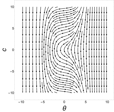
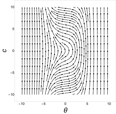
Figure 1: Phase portrait of vertical subsystem (34) for $C^{+}$ and $C^{-}$ (timelike case)

Let us introduce the energy integral:

$$E=\frac{h_{3}^{2}}{2}-h_{2}h_{4}=\frac{c^{2}}{2}-\alpha\sinh\theta,\qquad\dot{E}=h_{3}\dot{h}_{3}-h_{4}\dot{h}_{2}=0.$$ (35)

The set of all normal extremal paths is parametrized by points of the set

$$C =T_{q_{0}}^{*}M\cap\{H=-1/2,h_{1}>0\}=\big{\{}(h_{1},h_{2},h_{3},h_{4})\in{\mathbb{R}}^{4}\leavevmode\nobreak\ |\leavevmode\nobreak\ h_{1}^{2}-h_{2}^{2}=1,h_{1}>0\big{\}}$$

$$=\big{\{}(\theta,c,\alpha)\in{\mathbb{R}}^{3}\big{\}}.$$

The set $C$ has the following decomposition into invariant sets of equations (31)–(33):

$$C =C_{0}^{0}\cup C^{0}\cup C^{+}\cup C^{-},\quad\lambda=(\theta,c,\alpha),$$

$$C_{0}^{0} =\{\lambda\in C\leavevmode\nobreak\ |\leavevmode\nobreak\ c=0,\alpha=0\},$$

$$C^{0} =\{\lambda\in C\leavevmode\nobreak\ |\leavevmode\nobreak\ c\neq 0,\alpha=0\},$$

$$C^{+} =\{\lambda\in C\leavevmode\nobreak\ |\leavevmode\nobreak\ \alpha>0\},$$

$$C^{-} =\{\lambda\in C\leavevmode\nobreak\ |\leavevmode\nobreak\ \alpha<0\}.$$

Consider the general case $\alpha\neq 0$. Trajectories of vertical subsystem (31)–(33) for $C^{+}$ and $C^{-}$ are symmetric (see Fig. 1). This symmetry (see Section 5.2) has the following description:

$$\varepsilon^{1}\colon(\alpha,c,\theta,x_{1},x_{2},y,z)\mapsto(-\alpha,-c,-\theta,x_{1},-x_{2},-y,-z).$$ (36)

Thus, it is enough to integrate the Hamiltonian system in the case $C^{+}$ due to the symmetry $\varepsilon^{1}$. We introduce new coordinates $(\varphi,E,\alpha)$ in the subset $C^{+}$ which rectify the vertical subsystem (31)–(33):

$$\ae=\sqrt{\frac{\sqrt{E^{2}+\alpha^{2}}}{2}},\qquad k^{2}=\frac{1}{2}+\frac{E}{4\ae^{2}}\in(0,1),$$

$$c=-2\ae\operatorname{sc}\nolimits(\ae\varphi)\operatorname{dn}\nolimits(\ae\varphi),\qquad \varphi\in\Big{(}-\frac{\operatorname{K}\nolimits}{\ae},\frac{\operatorname{K}\nolimits}{\ae}\Big{)},$$

$$\sinh\theta=\frac{2\ae^{2}\Big{(}1-k^{2}\big{(}1+\operatorname{cn}\nolimits^{4}(\ae\varphi)\big{)}\Big{)}}{\alpha\operatorname{cn}\nolimits^{2}(\ae\varphi)},\qquad \cosh\theta=\frac{2\ae^{2}\Big{(}1-k^{2}\big{(}1-\operatorname{cn}\nolimits^{4}(\ae\varphi)\big{)}\Big{)}}{\alpha\operatorname{cn}\nolimits^{2}(\ae\varphi)},$$

where $\operatorname{sn}\nolimits\psi,\operatorname{cn}\nolimits\psi,\operatorname{dn}\nolimits\psi$ are elliptic Jacobi functions with modulus $k$, and $\displaystyle\operatorname{sc}\nolimits\psi=\frac{\operatorname{sn}\nolimits\psi}{\operatorname{cn}\nolimits\psi}$; $\displaystyle\operatorname{K}\nolimits(k)=\int_{0}^{\frac{\pi}{2}}\frac{dt}{\sqrt{1-k^{2}\sin^{2}t}}$ is the complete elliptic integral of the first kind.

Immediate differentiation shows that in these coordinates the subsystem for the costate variables (31)–(33) takes the following form:

$$\dot{\varphi}=1,\qquad\dot{E}=0,\qquad\dot{\alpha}=0,$$ (37)

so that it has the solutions

$$\varphi(t)=\varphi_{t}=\varphi_{0}+t,\qquad E=\operatorname{const}\nolimits,\qquad\alpha=\operatorname{const}\nolimits.$$ (38)

5.1 Exponential mapping for timelike normal extremals

Denote arguments of Jacobi functions $\psi_{0}=\ae\varphi_{0},\ \psi_{t}=\ae\varphi_{t}\in(-\operatorname{K}\nolimits,\operatorname{K}\nolimits)$ to describe the exponential mapping in general case $\alpha\neq 0$:

$$x_{1}(t) =\frac{2\ae}{|\alpha|}(\operatorname{sc}\nolimits\psi_{0}\operatorname{dn}\nolimits\psi_{0}-\operatorname{sc}\nolimits\psi_{t}\operatorname{dn}\nolimits\psi_{t}),$$ (39)

$$x_{2}(t) =\frac{4\ae\Big{(}\ae(1-k^{2})t-\big{(}\operatorname{E}\nolimits(\psi_{t})-\operatorname{E}\nolimits(\psi_{0})\big{)}\Big{)}-|\alpha|x_{1}(t)}{\alpha}.$$ (40)

$$y(t) =-\frac{2\ae^{2}}{\alpha|\alpha|}\Big{(}k^{2}(\operatorname{cn}\nolimits^{2}\psi_{t}-\operatorname{cn}\nolimits^{2}\psi_{0})+(1-k^{2})(\operatorname{nc}\nolimits^{2}\psi_{t}-\operatorname{nc}\nolimits^{2}\psi_{0})\Big{)}$$

$$\qquad+\frac{\ae}{|\alpha|}\Big{(}\operatorname{dn}\nolimits\psi_{0}\operatorname{sc}\nolimits\psi_{0}+\operatorname{dn}\nolimits\psi_{t}\operatorname{sc}\nolimits\psi_{t}\Big{)}x_{2}(t),$$ (41)

$$z(t) =\frac{\big{(}x_{2}(t)\big{)}^{3}}{6}+\frac{4\ae^{3}}{3\alpha^{3}}\bigg{(}2\ae(k^{2}-1)t+(1-k^{2})\Big{(}\frac{\operatorname{dn}\nolimits\psi_{t}\operatorname{sn}\nolimits\psi_{t}}{\operatorname{cn}\nolimits^{3}\psi_{t}}-\frac{\operatorname{dn}\nolimits\psi_{0}\operatorname{sn}\nolimits\psi_{0}}{\operatorname{cn}\nolimits^{3}\psi_{0}}\Big{)}$$

$$\qquad+k^{2}(\operatorname{cn}\nolimits\psi_{t}\operatorname{dn}\nolimits\psi_{t}\operatorname{sn}\nolimits\psi_{t}-\operatorname{cn}\nolimits\psi_{0}\operatorname{dn}\nolimits\psi_{0}\operatorname{sn}\nolimits\psi_{0})-2\big{(}\operatorname{E}\nolimits(\psi_{t})-\operatorname{E}\nolimits(\psi_{0})\big{)}(2k^{2}-1)\bigg{)}$$

$$\qquad-\frac{2\ae\operatorname{dn}\nolimits\psi_{0}\operatorname{sn}\nolimits\psi_{0}\Big{(}\frac{\ae\operatorname{dn}\nolimits\psi_{0}\operatorname{sc}\nolimits\psi_{0}}{|\alpha|}x_{2}(t)-\frac{1}{2}x_{1}(t)x_{2}(t)-y(t)\Big{)}}{\operatorname{cn}\nolimits\psi_{0}|\alpha|}$$

$$\qquad-\frac{2\ae^{2}(2k^{2}-1)x_{1}(t)}{3\alpha|\alpha|},$$ (42)

where $\displaystyle\operatorname{E}\nolimits(\psi)=\int_{0}^{\psi}\operatorname{dn}\nolimits^{2}t\ dt$.

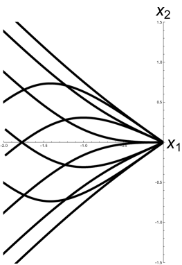
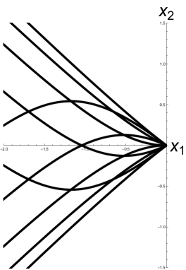
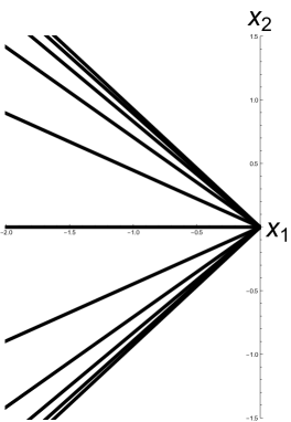
Figure 2: Projections of extremals to the plane $(x_{1},x_{2})$ for $C^{\pm}$, $C^{0}$ and $C_{0}^{0}$ (timelike case)

Projections of extremals to the plane $(x_{1},x_{2})$ with $|\alpha|=1$ and $\psi_{0}=0$ are shown in Fig. 2, left. Notice that since $\psi_{t}\in(-\operatorname{K}\nolimits,\operatorname{K}\nolimits)$ we have an upper bound for the time parameter

$$t<t_{\operatorname{supr}}(\lambda)=\frac{\operatorname{K}\nolimits(k)-\psi_{0}}{\ae}.$$ (43)

When $t\to t_{\operatorname{supr}}(\lambda)$, solutions (39)–(42) explode, i.e., tend to infinity.

For the subset $C^{0}$ we have

$$\alpha =0,\quad E=\frac{c^{2}}{2}\leavevmode\nobreak\ \Longrightarrow\quad c\equiv\operatorname{const}\nolimits,\ \theta=\theta_{0}-c\,t,$$

$$x_{1}(t) =\frac{\sinh(\theta_{0}-c\,t)-\sinh\theta_{0}}{c},$$

$$x_{2}(t) =\frac{\cosh\theta_{0}-\cosh(\theta_{0}-c\,t)}{c},$$

$$y(t) =\frac{\sinh(c\,t)-c\ t}{2c^{2}},$$

$$z(t) =\frac{4\sinh^{3}\big{(}\frac{c\,t}{2}\big{)}\sinh\big{(}3\theta_{0}-\frac{3c\,t}{2}\big{)}-3\big{(}\sinh(c\,t)-c\,t\big{)}\sinh\theta_{0}}{6c^{3}}.$$

Projections of extremals to the plane $(x_{1},x_{2})$ with $|c|=1$ (hyperbolas) are shown in Fig. 2, center.

If $\lambda\in C_{0}^{0}$, then

$$\alpha =c=E=0,\quad\theta\equiv\operatorname{const}\nolimits,\quad\sinh\theta=s_{0},\quad\cosh\theta=c_{0},$$

$$x_{1}(t) =-c_{0}\ t,$$

$$x_{2}(t) =s_{0}\ t,$$

$$y(t) \equiv 0,$$

$$z(t) =\frac{(2s_{0}^{2}+1)s_{0}}{6}\ t^{3}.$$

Projections of extremals to the plane $(x_{1},x_{2})$ are straight lines (see Fig. 2, right). For $\lambda\in C^{0}\cup C_{0}^{0}$ we have no upper bound for the time parameter: $t_{\operatorname{supr}}(\lambda)=+\infty$.

So we obtained a parameterization of the exponential mapping

$$\operatorname{Exp}\nolimits:N\to M={\mathbb{R}}^{4},\qquad\operatorname{Exp}\nolimits(\lambda,t)=q(t),$$ (44)

$$N=\{(\lambda,t)\in C\times{\mathbb{R}}_{+}\leavevmode\nobreak\ |\leavevmode\nobreak\ t\in\big{(}0,t_{\operatorname{supr}}(\lambda)\big{)}\},$$ (45)

in the timelike case. It maps a pair $(\lambda,t)$ to the point of the corresponding extremal trajectory $q(t)$.

Further we investigate discrete symmetries of the exponential mapping and on this basis find estimates for the cut time on extremals.

5.2 Discrete symmetries of exponential mapping

Subsystem (31)–(33) for costate variables of the normal Hamiltonian system has symmetries which preserve the direction field of this system. We already described one of them (36).

Let us define the action of symmetries $\varepsilon^{i}$ on the set of trajectories of the vertical subsystem with preservation of time direction. Denote a smooth curve

$$\gamma=\Big{\{}\big{(}\theta(t),c(t),\alpha\big{)}\leavevmode\nobreak\ |\leavevmode\nobreak\ t\in[0,T]\Big{\}}\subset C.$$

Define the action of symmetries on these curves (see. Fig. 3):

$$\varepsilon^{1}:\gamma\mapsto\gamma_{1}=\Big{\{}\big{(}\theta^{1}(t),c^{1}(t),\alpha^{1}\big{)}\leavevmode\nobreak\ |\leavevmode\nobreak\ t\in[0,T]\Big{\}}=\Big{\{}\big{(}-\theta(t),-c(t),-\alpha\big{)}\Big{\}},$$

$$\varepsilon^{2}:\gamma\mapsto\gamma_{2}=\Big{\{}\big{(}\theta^{2}(t),c^{2}(t),\alpha^{2}\big{)}\leavevmode\nobreak\ |\leavevmode\nobreak\ t\in[0,T]\Big{\}}=\Big{\{}\big{(}\theta(T-t),-c(T-t),\alpha\big{)}\Big{\}},$$

$$\varepsilon^{3}:\gamma\mapsto\gamma_{3}=\Big{\{}\big{(}\theta^{3}(t),c^{3}(t),\alpha^{3}\big{)}\leavevmode\nobreak\ |\leavevmode\nobreak\ t\in[0,T]\Big{\}}=\Big{\{}\big{(}-\theta(T-t),c(T-t),-\alpha\big{)}\Big{\}}.$$

It is obvious that if $\gamma$ is a solution to the vertical subsystem (31)–(33), then $\gamma_{i},i=1,2,3$, is a solution as well.

Now consider the group of symmetries $G=\{\mathrm{Id},\varepsilon^{1},\varepsilon^{2},\varepsilon^{3}=\varepsilon^{1}\circ\varepsilon^{2}\}\cong{\mathbb{Z}}_{2}\times{\mathbb{Z}}_{2}$. The symmetry $\varepsilon^{1}$ preserves the direction of time, while $\varepsilon^{2}$ and $\varepsilon^{3}$ change it.

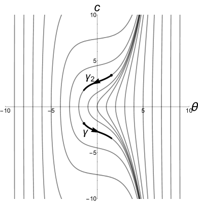
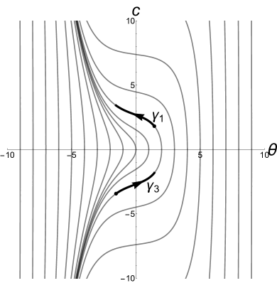
Figure 3: Action of symmetries on trajectories of vertical subsystem (timelike case)

Continue the action of symmetries from the vertical subsystem to solutions of the Hamiltonian system of PMP

$$\dot{\theta}(t)=-c(t),\quad\dot{c}(t)=-\alpha\cosh\theta(t),\quad\dot{\alpha}=0,$$ (46)

$$\dot{q}(t)=-\cosh\theta(t)X_{1}\big{(}q(t)\big{)}+\sinh\theta(t)X_{2}\big{(}q(t)\big{)},$$ (47)

in the following way:

$$\varepsilon^{i}:\Big{\{}\big{(}\theta(t),c(t),\alpha,q(t)\big{)}\leavevmode\nobreak\ |\leavevmode\nobreak\ t\in[0,T]\Big{\}}\mapsto\Big{\{}\big{(}\theta^{i}(t),c^{i}(t),\alpha^{i},q^{i}(t)\big{)}|t\in[0,T]\Big{\}},$$ (48)

where $q(t)=\big{(}x_{1}(t),x_{2}(t),y(t),z(t)\big{)},\ t\in[0,T],$ is a geodesic and

$$q^{i}(t)=\big{(}x_{1}^{i}(t),x_{2}^{i}(t),y^{i}(t),z^{i}(t)\big{)},\qquad t\in[0,T],\ i=1,2,3,$$

are its images under the action of the symmetries $\varepsilon^{i}$.

Lemma 1.

The symmetries $\varepsilon^{i}$ map trajectories on the plane $(x_{1},x_{2})$ in the following way:

$$x_{1}^{1}(t)=x_{1}(t),\qquad x_{2}^{1}(t)=-x_{2}(t),$$

$$x_{1}^{2}(t)=x_{1}(T)-x_{1}(T-t),\qquad x_{2}^{2}(t)=x_{2}(T)-x_{2}(T-t),$$

$$x_{1}^{3}(t)=x_{1}(T)-x_{1}(T-t),\qquad x_{2}^{3}(t)=x_{2}(T-t)-x_{2}(T).$$

Proof.

Via direct integration, for instance, for $\varepsilon^{2}$ we verify that

$$x_{1}^{2}(t)=\int_{0}^{t}\big{(}-\cosh\theta(T-s)\big{)}ds=\int_{T-t}^{T}\big{(}-\cosh\theta(r)\big{)}dr=x_{1}(T)-x_{1}(T-t),$$

$$x_{2}^{2}(t)=\int_{0}^{t}\sinh\theta(T-s)ds=\int_{T-t}^{T}\sinh\theta(r)dr=x_{2}(T)-x_{2}(T-t).$$

∎

Lemma 2.

The symmetries $\varepsilon^{i}$ map endpoints of geodesics $q=(x_{1},x_{2},y,z)$ to endpoints of $q^{i}=(x_{1}^{i},x_{2}^{i},y^{i},z^{i}\big{)}$ in the following way:

$$x_{1}^{1}(T)=x_{1}(T), x_{2}^{1}(T)=-x_{2}(T), y^{1}(T)=-y(T), z^{1}(T)=-z(T),$$

$$x_{1}^{2}(T)=x_{1}(T), x_{2}^{2}(T)=x_{2}(T), y^{2}(T)=-y(T), z^{2}(T)=z(T)-x_{1}(T)y(T),$$

$$x_{1}^{3}(T)=x_{1}(T), x_{2}^{3}(T)=-x_{2}(T), y^{3}(T)=y(T), z^{3}(T)=-z(T)+x_{1}(T)y(T).$$

Proof.

Lemma 1 gives us the expressions for $x_{1}^{i}(T)$ and $x_{2}^{i}(T)$. The expressions for other variables are obtained by integration. For example, for $\varepsilon^{2}$ we have

$$y^{2}(T) =\int_{0}^{T}\frac{x_{2}^{2}(t)\cosh\theta^{2}(t)+x_{1}^{2}(t)\sinh\theta^{2}(t)}{2}dt=\frac{x_{2}(T)}{2}\int_{0}^{T}\cos\theta(T-t)dt$$

$$\qquad\quad+\frac{x_{1}(T)}{2}\int_{0}^{T}\sinh\theta(T-t)dt-\int_{0}^{T}\frac{x_{2}(s)\cosh\theta(s)+x_{1}(s)\sinh\theta(s)}{2}ds$$

$$\qquad=\frac{x_{2}(T)x_{1}(T)}{2}-\frac{x_{1}(T)x_{2}(T)}{2}-y(T)=-y(T),$$

$$z^{2}(T) =\int_{0}^{T}\frac{\big{(}x_{1}^{2}(t)\big{)}^{2}+\big{(}x_{2}^{2}(t)\big{)}^{2}}{2}\dot{x}_{2}^{2}(t)dt=\frac{\big{(}x_{2}^{2}(T)\big{)}^{3}}{6}+\int_{0}^{T}\frac{\big{(}x_{1}^{2}(t)\big{)}^{2}}{2}\dot{x}_{2}^{2}(t)dt$$

$$\qquad=\frac{\big{(}x_{2}(T)\big{)}^{3}}{2}+\int_{0}^{T}\frac{\big{(}x_{1}(T)\big{)}^{2}-2x_{1}(T)x_{1}(T-t)+\big{(}x_{1}(T-t)\big{)}^{2}}{2}\dot{x}_{2}(T-t)dt$$

$$\qquad=\frac{\big{(}x_{2}(T)\big{)}^{3}}{6}+\frac{\big{(}x_{1}(T)\big{)}^{2}x_{2}(T)}{2}-x_{1}(T)\int_{0}^{T}x_{1}(s)\dot{x}_{2}(s)ds+z(T)-\frac{\big{(}x_{2}(T)\big{)}^{3}}{6}$$

$$\qquad=\frac{\big{(}x_{1}(T)\big{)}^{2}x_{2}(T)}{2}-x_{1}(T)\Big{(}y(T)+\frac{x_{1}(T)x_{2}(T)}{2}\Big{)}+z(T)=z(T)-x_{1}(T)y(T).$$

∎

We define the action of $\varepsilon^{i}$ in the preimage $N$ of the exponential mapping by restricting the action to initial point of trajectory of vertical subsystem:

$$\varepsilon^{i}:C\to C,\qquad\varepsilon^{i}(\theta,c,\alpha)=(\theta^{i},c^{i},\alpha^{i}),$$ (49)

$$(\theta^{1},c^{1},\alpha^{1})=(-\theta,-c,-\alpha),$$ (50)

$$(\theta^{2},c^{2},\alpha^{2})=(\theta,-c,\alpha),$$ (51)

$$(\theta^{3},c^{3},\alpha^{3})=(-\theta,c,-\alpha),$$ (52)

in the following way:

$$\varepsilon^{1}(\lambda,t)=\big{(}\varepsilon^{1}(\lambda),t\big{)},$$

$$\varepsilon^{i}(\lambda,t)=\big{(}\varepsilon^{i}\circ e^{t\vec{H}_{v}}(\lambda),t\big{)},\qquad i=2,3,$$

where $\vec{H}_{v}=-c\frac{\partial}{\partial\theta}-\alpha\cosh\theta\frac{\partial}{\partial c}\in\mathrm{Vec}(C)$ is the vertical part of Hamiltonian vector field.

We define the action of $\varepsilon^{i}$ in the image of exponential mapping $M$ by restricting the action to endpoints of extremals (see Lemma 2):

$$\varepsilon^{i}:M\to M,\qquad\varepsilon^{i}(q)=\varepsilon^{i}(x_{1},x_{2},y,z)=q^{i}=(x_{1}^{i},x_{2}^{i},y^{i},z^{i}),$$ (53)

$$(x_{1}^{1},x_{2}^{1},y^{1},z^{1})=(x_{1},\ -x_{2},\ -y,\ -z),$$ (54)

$$(x_{1}^{2},x_{2}^{2},y^{2},z^{2})=(x_{1},\ x_{2},\ -y,\ z-x_{1}y),$$ (55)

$$(x_{1}^{3},x_{2}^{3},y^{3},z^{3})=(x_{1},\ -x_{2},\ y,\ x_{1}y-z).$$ (56)

Since the action of $\varepsilon^{i}$ in the domain $N$ and the image $M$ of the exponential map are induced by the actions of symmetries (48) on trajectories of the Hamiltonian system (46)–(47), we have the following result.

Proposition 1.

The mappings $\varepsilon^{i},i=1,2,3,$ are symmetries of the exponential mapping, i.e.,

$$(\varepsilon^{i}\circ\operatorname{Exp}\nolimits)(\theta,c,\alpha,t)=(\operatorname{Exp}\nolimits\circ\,\varepsilon^{i})(\theta,c,\alpha,t),\qquad(\theta,c,\alpha,t)\in N.$$

5.3 Maxwell points of timelike normal extremals

A point $q(t)$ on a geodesic is called a Maxwell point if there exists another geodesic $\tilde{q}(s)\not\equiv q(s)$ for which $\tilde{q}(t)=q(t),t>0$. It is known that a geodesic cannot be optimal after a Maxwell point. In this section we compute the Maxwell points corresponding to some symmetries $\varepsilon^{i}$. On this basis we derive estimates for the cut time along geodesics

$$t_{\operatorname{cut}}(\lambda)=\sup\{t>0\leavevmode\nobreak\ |\leavevmode\nobreak\ \operatorname{Exp}\nolimits(\lambda,s)\text{ is optimal for }s\in[0,t]\}.$$

We define Maxwell sets in the preimage of $\operatorname{Exp}\nolimits$ corresponding to the symmetries $\varepsilon^{i}$:

$$\operatorname{MAX}\nolimits^{i} =\big{\{}(\lambda,t)\in N\leavevmode\nobreak\ |\leavevmode\nobreak\ \lambda^{i}\neq\lambda,\ \operatorname{Exp}\nolimits(\lambda^{i},t)=\operatorname{Exp}\nolimits(\lambda,t)\big{\}},$$ (57)

$$\lambda =(\theta,c,\alpha),\qquad\lambda^{i}=\varepsilon^{i}(\lambda).$$

It follows from Proposition 1 that the equality $\operatorname{Exp}\nolimits(\lambda^{i},t)=\operatorname{Exp}\nolimits(\lambda,t)$ is equivalent to $\varepsilon^{i}\big{(}q(t)\big{)}=q(t)$. Therefore we get a description of fixed points of the symmetries $\varepsilon^{i}$ in the image of the exponential mapping.

Lemma 3.

1. $\varepsilon^{1}(q)=q\quad\Longleftrightarrow\quad x_{2}=0,\ y=0,\ z=0$.

2. $\varepsilon^{2}(q)=q\quad\Longleftrightarrow\quad y=0$.

3. $\displaystyle\varepsilon^{3}(q)=q\quad\Longleftrightarrow\quad x_{2}=0,\ z=\frac{x_{1}y}{2}$.

Proof.

Follows from definition (53)–(56) of action of the symmetries in $E$. ∎

Now we compute fixed points of symmetries in the preimage of exponential mapping, which is necessary for description of Maxwell sets. Introduce the following coordinates in the sets $N^{\pm}=\{(\lambda,t)\in C^{\pm}\times{\mathbb{R}}_{+}\mid t\in\big{(}0,t_{\operatorname{supr}}(\lambda)\big{)}\}$:

$$\tau=\frac{\psi_{t}+\psi_{0}}{2},\qquad p=\frac{\psi_{t}-\psi_{0}}{2}=\frac{\ae t}{2}.$$ (58)

The parameter $\tau$ corresponds to the middle point of a trajectory.

Lemma 4.

1. $\lambda^{1}=\lambda\quad\Longleftrightarrow\quad\lambda\in C_{0}^{0},\ \theta=0.$

2. $\lambda^{2}=\lambda\quad\Longleftrightarrow\quad\lambda\in C^{\pm},\tau=0$  or  $\lambda\in C_{0}^{0}$.

3. $\displaystyle\lambda^{3}=\lambda\quad\Longleftrightarrow\quad\lambda\in C^{0}\cup C_{0}^{0},\ \theta+\frac{ct}{2}=0$

Proof.

Follows from the definition of action of reflections in the domain of exponential mapping (49)–(52). ∎

Theorem 4.

Let $(\lambda,T)\in N$ and $q(T)=\operatorname{Exp}\nolimits(\lambda,T)$. Then

1. $(\lambda,T)\in\operatorname{MAX}\nolimits^{1}\quad\Longleftrightarrow\quad x_{2}(T)=y(T)=z(T)=0$  and  if $\lambda\in C_{0}^{0}$, then $\theta\neq 0$.

2. $(\lambda,T)\in\operatorname{MAX}\nolimits^{2}\quad\Longleftrightarrow\quad\lambda\in C^{\pm},y(T)=0,\tau\neq 0$  or  $\lambda\in C^{0},y(T)=0$.

3. $(\lambda,T)\in\operatorname{MAX}\nolimits^{3}\quad\Longleftrightarrow\quad x_{2}=0,\displaystyle z=\frac{x_{1}y}{2}$ and if $\lambda\in C^{0}\cup C_{0}^{0}$, then $\displaystyle\theta\neq-\frac{ct}{2}$.

Proof.

Follows from definition (57) of Maxwell sets, Lemmas 3 and 4. ∎

The equations $\varepsilon^{i}(q)=q$  define sub-manifolds in ${\mathbb{R}}^{4}$ with dimension from 3 to 1, exponential mapping translates the corresponding Maxwell sets into these sub-manifolds:

$$\operatorname{Exp}\nolimits(\operatorname{MAX}\nolimits^{i})\subset\{q\in M\leavevmode\nobreak\ |\leavevmode\nobreak\ \varepsilon^{i}(q)=q\},\qquad i=1,2,3.$$

Further we describe in details the set $\operatorname{MAX}\nolimits^{2}$ since it defines a sub-manifold in $M$ with the maximum dimension 3, while $\operatorname{MAX}\nolimits^{1}$ and $\operatorname{MAX}\nolimits^{3}$ define sub-manifolds with dimension 1 and 2. Using new coordinates (58) in the case $\alpha\neq 0$ we get

$$y =-\frac{\operatorname{sn}\nolimits\tau\operatorname{cn}\nolimits\tau\operatorname{dn}\nolimits\tau f_{y}(p)}{\alpha|\alpha|\ae^{2}k^{2}(\operatorname{cn}\nolimits^{2}\tau-\operatorname{dn}\nolimits^{2}\tau\operatorname{sn}\nolimits^{2}p)(1-k^{2}\operatorname{sn}\nolimits^{2}p\operatorname{sn}\nolimits^{2}\tau)},$$

$$f_{y}(p) =-16\ae^{4}k^{4}\operatorname{cn}\nolimits^{3}p\operatorname{dn}\nolimits p\operatorname{sn}\nolimits p+(16\ae^{4}k^{2}\operatorname{E}\nolimits(p)-\alpha^{2}p)(\operatorname{dn}\nolimits^{2}p-k^{2}\operatorname{cn}\nolimits^{2}p\operatorname{sn}\nolimits^{2}p).$$

This gives us a description of the Maxwell set:

$$\operatorname{MAX}\nolimits^{2}\cap N^{\pm} =\{\nu\in N^{\pm}\leavevmode\nobreak\ |\leavevmode\nobreak\ y(\nu)=0,\tau\neq 0,\tau\in(-\operatorname{K}\nolimits,\operatorname{K}\nolimits),p\in(0,\operatorname{K}\nolimits)\}$$

$$=\{\nu\in N^{\pm}\leavevmode\nobreak\ |\leavevmode\nobreak\ f_{y}(p)=0,p\in(0,\operatorname{K}\nolimits)\},$$ (59)

where $\nu=(\tau,p,E,\alpha)$.

The following obvious lemma will be useful for localization of roots of functions.

Lemma 5.

Let smooth functions $f(u),g(u)$ satisfy on $(0,u_{0})\subset{\mathbb{R}}$ the conditions

$$f(u)\not\equiv 0,\quad g(u)>0,\quad\bigg{(}\frac{f(u)}{g(u)}\bigg{)}^{\prime}\geq 0,$$ (60)

$$\lim_{u\to 0}\frac{f(u)}{g(u)}=0.$$ (61)

Then $f(u)>0$ for $u\in(0,u_{0})$.

If functions $f$ and $g$ satisfy conditions (60), (61), then we say that $g$ is a comparison function for $f$ on the interval $(0,u_{0})$.

Lemma 6.

The function $f_{y}(p)>0$ for $p\in\big{(}0,\operatorname{K}\nolimits(k)\big{)},\ k\in(0,1)$.

Proof.

We show that the function $g(p)=k^{2}\big{(}1-k^{2}(1-\operatorname{cn}\nolimits^{4}p)\big{)}$ is a comparison function for $f_{y}(p)$ for $p\in(0,\operatorname{K}\nolimits)$.

The inequality $f_{y}(p)\not\equiv 0$ follows from the expansion $f_{y}(p)=\frac{4}{3}\alpha^{2}k^{2}p^{3}+o(p^{3})$. Notice that $g(p)>0$ for $p\in(0,\operatorname{K}\nolimits)$. Finally we get the equalities

$$\bigg{(}\frac{f_{y}(p)}{g(p)}\bigg{)}^{\prime}=\frac{4\alpha^{2}\operatorname{sn}\nolimits^{2}p\operatorname{cn}\nolimits^{2}p\operatorname{dn}\nolimits p}{1-k^{2}(1-\operatorname{cn}\nolimits^{4}p)}>0,\quad\frac{f_{y}(p)}{g(p)}=\frac{4}{3}\alpha^{2}p^{3}+o(p^{3}).$$

So $g(p)$ is a comparison function for $f_{y}(p)$; thus, it follows from Lemma 5 that $f_{y}(p)>0$ for $p\in(0,\operatorname{K}\nolimits)$. ∎

Theorem 5.

$\operatorname{MAX}\nolimits^{2}\cap N^{\pm}=\emptyset.$

Proof.

Follows immediately from description of Maxwell set (59) and Lemma 6. ∎

We proved that a general geodesic with $\lambda\in C^{\pm}$ has no Maxwell times $t_{\operatorname{MAX}\nolimits}(\lambda)\in\big{(}0,t_{\operatorname{supr}}(\lambda)\big{)}$ corresponding to the symmetries $\varepsilon^{i},i=1,2,3$. So we conjecture that geodesics $q(t)=\operatorname{Exp}\nolimits(\lambda,t)$ with $\lambda\in C^{\pm}$ are optimal for $t\in\big{(}0,t_{\operatorname{supr}}(\lambda)\big{)}$.

6 Spacelike normal extremal trajectories

In the spacelike case $H=\frac{1}{2}\big{(}-h_{1}^{2}+h_{2}^{2}\big{)}>0,$ we consider extremals on the level surface $H=1/2$ and introduce new coordinates on this surface:

$$h_{1}=\sinh\theta,\quad\ h_{2}=\pm\cosh\theta,\quad h_{3}=c,\quad\ h_{4}=\alpha.$$

Notice that we have the following symmetry of the Hamiltonian system:

$$\varepsilon^{0}:(h_{1},h_{2},h_{3},h_{4},x_{1},x_{2},y,z)\mapsto(h_{1},-h_{2},-h_{3},-h_{4},x_{1},-x_{2},-y,-z),$$ (62)

So we assume $h_{2}=\cosh\theta>0$ without loss of generality in the sequel.

In the variables $(\theta,c,\alpha,x_{1},x_{2},y,z)$ on the level surface $\{H=1/2\}$ the Hamiltonian system of Pontryagin maximum principle takes the following form in the normal case for spacelike curves:

$$\dot{x}_{1}=-\sinh\theta,$$ (63)

$$\dot{x}_{2}=\cosh\theta,$$ (64)

$$\dot{y}=\frac{x_{2}\sinh\theta+x_{1}\cosh\theta}{2},$$ (65)

$$\dot{z}=\frac{x_{1}^{2}+x_{2}^{2}}{2}\cosh\theta,$$ (66)

$$\dot{\theta}=-c,$$ (67)

$$\dot{c}=-\alpha\sinh\theta,$$ (68)

$$\dot{\alpha}=0.$$ (69)

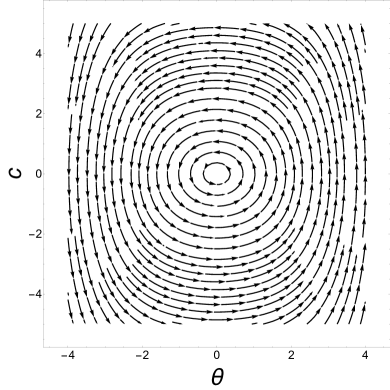
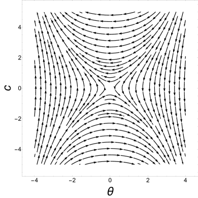
Figure 4: Phase portraits of the vertical subsystem for $\alpha=-1,\ 1$ (spacelike case)

The vertical subsystem (67)–(69) has the energy integral:

$$E=\frac{h_{3}^{2}}{2}-h_{2}h_{4}=\frac{c^{2}}{2}-\alpha\cosh\theta.$$ (70)

The family of all normal extremals is parametrized by points of the set

$$C =T_{q_{0}}^{*}\cap\{H=1/2,h_{2}>0\}=\big{\{}(h_{1},h_{2},h_{3},h_{4})\in{\mathbb{R}}^{4}\leavevmode\nobreak\ |\leavevmode\nobreak\ h_{2}^{2}-h_{1}^{2}=1,h_{2}>0\big{\}}$$

$$=\big{\{}(\theta,c,\alpha)\in{\mathbb{R}}^{3}\big{\}}.$$

The set $C$ has the following decomposition into invariant sets of equations (67)–(69):

$$C =\cup_{i=1}^{7}C_{i},\quad C_{i}\cap C_{j}=\emptyset,\ i\neq j,\qquad\lambda=(\theta,c,\alpha),$$

$$C_{1} =\{\lambda\in C\leavevmode\nobreak\ |\leavevmode\nobreak\ \alpha<0,E>-\alpha\},$$

$$C_{2} =\{\lambda\in C\leavevmode\nobreak\ |\leavevmode\nobreak\ \alpha>0,E<-\alpha\},$$

$$C_{3} =\{\lambda\in C\leavevmode\nobreak\ |\leavevmode\nobreak\ \alpha>0,E>-\alpha\},$$

$$C_{4} =\{\lambda\in C\leavevmode\nobreak\ |\leavevmode\nobreak\ \alpha>0,E=-\alpha,\ c\neq 0,\theta\neq 0\},$$

$$C_{5} =\{\lambda\in C\leavevmode\nobreak\ |\leavevmode\nobreak\ \alpha\neq 0,E=-\alpha,\ c=0,\theta=0\},$$

$$C_{6} =\{\lambda\in C\leavevmode\nobreak\ |\leavevmode\nobreak\ \alpha=0,\ E>0,c\neq 0\},$$

$$C_{7} =\{\lambda\in C\leavevmode\nobreak\ |\leavevmode\nobreak\ \alpha=0,\ E=0,c=0\}.$$

In order to parameterize extremals, we introduce coordinates $(\varphi,E,\alpha)$ on the set $\bigcup_{i=1}^{3}C_{i}$ in the following way.

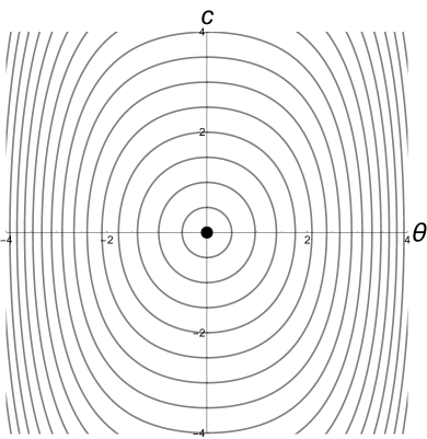
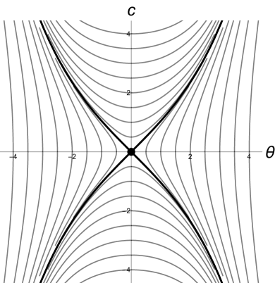
Figure 5: Trajectories of the vertical subsystem for $\alpha=-1,\ 1$ (spacelike case)

In the domain $C_{1}$:

$$k =\sqrt{\frac{E+\alpha}{E-\alpha}}\in(0,1),\qquad \ae=\sqrt{\frac{E-\alpha}{2}},$$

$$c =\sqrt{2(E+\alpha)}\operatorname{sn}\nolimits(\ae\varphi),\qquad \varphi\in{\mathbb{R}},$$

$$\sinh\theta =\frac{\sqrt{E-\alpha}\ \sqrt{E+\alpha}\operatorname{cn}\nolimits(\ae\varphi)\operatorname{dn}\nolimits(\ae\varphi)}{\alpha},\qquad \cosh\theta=1-\frac{(E+\alpha)\operatorname{cn}\nolimits^{2}(\ae\varphi)}{\alpha}.$$

In the domain $C_{2}$:

$$k =\sqrt{\frac{2\alpha}{\alpha-E}}\in(0,1),\qquad \ae=\sqrt{\frac{\alpha-E}{2}},$$

$$c =\operatorname{sgn}\nolimits\theta\frac{\sqrt{2(-\alpha-E)}\operatorname{sn}\nolimits(\ae\varphi)}{\operatorname{cn}\nolimits(\ae\varphi)},\qquad \varphi\in\Big{(}-\frac{\operatorname{K}\nolimits}{\ae},\frac{\operatorname{K}\nolimits}{\ae}\Big{)},$$

$$\sinh\theta =\operatorname{sgn}\nolimits\theta\frac{\sqrt{-\alpha-E}\ \sqrt{\alpha-E}\operatorname{dn}\nolimits(\ae\varphi)}{\alpha\operatorname{cn}\nolimits^{2}(\ae\varphi)},\qquad \cosh\theta=1-\frac{\alpha+E}{\alpha\operatorname{cn}\nolimits(\ae\varphi)}.$$

In the domain $C_{3}$:

$$k =\sqrt{\frac{E-\alpha}{E+\alpha}}\quad k_{2}=k^{2}\in(-\infty,1),\qquad \ae=\sqrt{\frac{E+\alpha}{2}},$$

$$c =\operatorname{sgn}\nolimits c\frac{2\ae\operatorname{dn}\nolimits(\ae\varphi)}{\operatorname{cn}\nolimits(\ae\varphi)},\qquad \varphi\in\Big{(}-\frac{\operatorname{K}\nolimits}{\ae},\frac{\operatorname{K}\nolimits}{\ae}\Big{)},$$

$$\sinh\theta =\operatorname{sgn}\nolimits c\frac{2\operatorname{sn}\nolimits(\ae\varphi)}{\operatorname{cn}\nolimits^{2}(\ae\varphi)},\qquad \cosh\theta=\frac{1+\operatorname{sn}\nolimits^{2}(\ae\varphi)}{\operatorname{cn}\nolimits^{2}(\ae\varphi)}.$$

Remark 2.

If $k^{2}<0$, then $\displaystyle k=i\frac{\tilde{k}}{\sqrt{1-\tilde{k}^{2}}},\tilde{k}=\sqrt{\frac{-k^{2}}{1-k^{2}}}\in(0,1).$ Using formulas from [8] we have

$$\tilde{k} =\sqrt{\frac{\alpha-E}{2\alpha}},\quad\sqrt{1-\tilde{k}^{2}}=\sqrt{\frac{\alpha+E}{2\alpha}};\quad \operatorname{dn}\nolimits(\ae\varphi,k) =\frac{1}{\operatorname{dn}\nolimits(\sqrt{\alpha}\varphi,\tilde{k})},$$ (71)

$$\operatorname{sn}\nolimits(\ae\varphi,k) =\frac{\sqrt{1-\tilde{k}^{2}}\operatorname{sn}\nolimits(\sqrt{\alpha}\varphi,\tilde{k})}{\operatorname{dn}\nolimits(\sqrt{\alpha}\varphi,\tilde{k})},\qquad \operatorname{cn}\nolimits(\ae\varphi,k) =\frac{\operatorname{cn}\nolimits(\sqrt{\alpha}\varphi,\tilde{k})}{\operatorname{dn}\nolimits(\sqrt{\alpha}\varphi,\tilde{k})}.$$ (72)

In the domain $C_{4}$:

$$c =\operatorname{sgn}\nolimits\theta\frac{4\alpha e^{\ae\varphi}}{\alpha e^{2\ae\varphi}-1},\qquad \ae=\sqrt{\alpha},\quad\varphi\in{\mathbb{R}},\ \alpha e^{2\ae\varphi}\neq 1,$$

$$\sinh\theta =\operatorname{sgn}\nolimits\theta\frac{4\ae e^{\ae\varphi}(\alpha e^{2\ae\varphi}+1)}{(\alpha e^{2\ae\varphi}-1)^{2}},\qquad \cos\theta=\frac{\alpha e^{2\ae\varphi}(\alpha e^{2\ae\varphi}+6)+1}{\alpha e^{2\ae\varphi}-1}.$$

Immediate differentiation shows that in the coordinates $(\varphi,E,\alpha)$ the subsystem for the costate variables (67)–(69) takes the following form:

$$\dot{\varphi}=1,\qquad\dot{E}=0,\qquad\dot{\alpha}=0,$$ (73)

so that it has solutions

$$\varphi(t)=\varphi_{t}=\varphi_{0}+t,\qquad E=\operatorname{const}\nolimits,\qquad\alpha=\operatorname{const}\nolimits.$$ (74)

6.1 Exponential mapping for spacelike normal extremals

Denote $\psi_{0}=\ae\varphi_{0},\psi_{t}=\ae\varphi_{t}$. From the definition of the variables $c$ and $\theta$ we obtain the following parametrization of extremal trajectories.

If $\lambda\in C_{1}$, then

$$x_{1}(t) =\frac{\sqrt{2}\sqrt{\alpha+E}}{\alpha}\Big{(}\operatorname{sn}\nolimits\psi_{t}-\operatorname{sn}\nolimits\psi_{0}\Big{)},$$ (75)

$$x_{2}(t) =-\frac{2\ae}{\alpha}\Big{(}\operatorname{E}\nolimits(\psi_{t})-\operatorname{E}\nolimits(\psi_{0})\Big{)}-t,$$ (76)

$$y(t) =\frac{\sqrt{\alpha+E}}{\sqrt{2}\alpha^{2}}\bigg{(}2\ae\Big{(}\operatorname{cn}\nolimits\psi_{t}\operatorname{dn}\nolimits\psi_{t}-\operatorname{cn}\nolimits\psi_{0}\operatorname{dn}\nolimits\psi_{0}+\big{(}\operatorname{E}\nolimits(\psi_{t})-\operatorname{E}\nolimits(\psi_{0})\big{)}\big{(}\operatorname{sn}\nolimits\psi_{t}+\operatorname{sn}\nolimits\psi_{0}\big{)}\Big{)}$$

$$\qquad+\alpha\Big{(}\operatorname{sn}\nolimits\psi_{t}+\operatorname{sn}\nolimits\psi_{0}\Big{)}t\bigg{)},$$ (77)

$$z(t) =\frac{\big{(}x_{2}(t)\big{)}^{3}}{6}+\frac{1}{3\alpha^{3}}\bigg{(}2\ae\Big{(}\big{(}\alpha+E\big{)}\big{(}\operatorname{cn}\nolimits\psi_{t}\operatorname{dn}\nolimits\psi_{t}(\operatorname{sn}\nolimits\psi_{t}-\operatorname{sn}\nolimits\psi_{0})$$

$$\qquad-2(\operatorname{cn}\nolimits\psi_{t}\operatorname{dn}\nolimits\psi_{t}-\operatorname{cn}\nolimits\psi_{0}\operatorname{dn}\nolimits\psi_{0})\operatorname{sn}\nolimits\psi_{0}\big{)}-\big{(}E+3(\alpha+E)\operatorname{sn}\nolimits^{2}\psi_{0}\big{)}\big{(}\operatorname{E}\nolimits(\psi_{t})$$

$$\qquad-\operatorname{E}\nolimits(\psi_{0})\big{)}\Big{)}+\alpha\Big{(}\alpha-E-3\big{(}\alpha+E\big{)}\operatorname{sn}\nolimits^{2}\psi_{0}\Big{)}t\bigg{)}.$$ (78)

Projections of extremals to the plane $(x_{1},x_{2})$ with $|\alpha|=1$ and $\psi_{0}=0$ are shown in Fig. 6, left. This case has no upper bounds for time: $t_{\operatorname{supr}}(\lambda)=+\infty$.

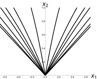
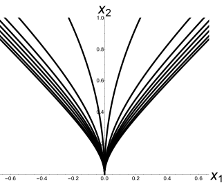
Figure 6: Projections of goedesics to the plane $(x_{1},x_{2})$ for $\lambda\in C_{1}$, $\lambda\in C_{2}$ and $\lambda\in C_{3}$ (spacelike case)

If $\lambda\in C_{2}$, then

$$x_{1}(t) =-\frac{\sqrt{2}\sqrt{-\alpha-E}\operatorname{sgn}\nolimits\theta}{\alpha}\Big{(}\operatorname{sc}\nolimits\psi_{t}-\operatorname{sc}\nolimits\psi_{0}\Big{)},$$ (79)

$$x_{2}(t) =-\frac{2\ae\big{(}\operatorname{E}\nolimits(\psi_{t})-\operatorname{E}\nolimits(\psi_{0})+\operatorname{dn}\nolimits\psi_{0}\operatorname{sc}\nolimits\psi_{0}-\operatorname{dn}\nolimits\psi_{t}\operatorname{sc}\nolimits\psi_{t}\big{)}+Et}{\alpha},$$ (80)

$$y(t) =-\frac{\sqrt{-\alpha-E}\operatorname{sgn}\nolimits\theta}{\sqrt{2}\alpha^{2}}\bigg{(}E\Big{(}\operatorname{sc}\nolimits\psi_{0}+\operatorname{sc}\nolimits\psi_{t}\Big{)}t+2\ae\Big{(}\big{(}\operatorname{sc}\nolimits\psi_{0}+\operatorname{sc}\nolimits\psi_{t}\big{)}\big{(}\operatorname{E}\nolimits(\psi_{t})-\operatorname{E}\nolimits(\psi_{0})\big{)}$$

$$\qquad+\big{(}\operatorname{dn}\nolimits\psi_{t}-\operatorname{dn}\nolimits\psi_{0}\big{)}\big{(}1-\operatorname{sc}\nolimits\psi_{0}\operatorname{sc}\nolimits\psi_{t}\big{)}\Big{)}\bigg{)},$$ (81)

$$z(t) =\frac{\big{(}x_{2}(t)\big{)}^{3}}{6}+\frac{2\ae\big{(}3(\alpha+E)\operatorname{sn}\nolimits^{2}\psi_{0}-E\operatorname{cn}\nolimits^{2}\psi_{0}\big{)}}{3\alpha^{3}\operatorname{cn}\nolimits^{2}\psi_{0}}\Big{(}\operatorname{E}\nolimits(\psi_{t})-\operatorname{E}\nolimits(\psi_{0})\Big{)}$$

$$\qquad+\frac{1}{3\alpha^{3}\ae\operatorname{cn}\nolimits^{3}\psi_{t}\operatorname{cn}\nolimits^{3}\psi_{0}}\Bigg{(}2\ae\bigg{(}\operatorname{cn}\nolimits\psi_{t}\Big{(}\alpha\big{(}\operatorname{cn}\nolimits^{2}\psi_{t}\operatorname{dn}\nolimits\psi_{0}(1-3\operatorname{cn}\nolimits^{2}\psi_{0})$$

$$\qquad+3\operatorname{cn}\nolimits^{2}\psi_{0}\operatorname{dn}\nolimits\psi_{t}\big{)}+\Big{(}\operatorname{cn}\nolimits^{2}\psi_{t}\operatorname{dn}\nolimits\psi_{0}\big{(}1-4\operatorname{cn}\nolimits^{2}\psi_{0}\big{)}+3\operatorname{cn}\nolimits^{2}\psi_{0}\operatorname{dn}\nolimits\psi_{t}\Big{)}E\bigg{)}\operatorname{sn}\nolimits\psi_{0}$$

$$\qquad-\operatorname{cn}\nolimits\psi_{0}\operatorname{dn}\nolimits\psi_{t}\bigg{(}\alpha\operatorname{cn}\nolimits^{2}\psi_{0}+3\alpha\operatorname{sn}\nolimits^{2}\psi_{0}\operatorname{cn}\nolimits^{2}\psi_{t}+\Big{(}3\operatorname{cn}\nolimits^{2}\psi_{t}+\operatorname{cn}\nolimits^{2}\psi_{0}\big{(}1$$

$$\qquad-4\operatorname{cn}\nolimits^{2}\psi_{t}\big{)}\Big{)}E\bigg{)}\operatorname{sn}\nolimits\psi_{t}\Bigg{)}+\frac{\big{(}\alpha+E\big{)}\big{(}\operatorname{cn}\nolimits^{2}\psi_{0}(\alpha-4E)+3E\big{)}}{3\alpha^{3}\operatorname{cn}\nolimits^{2}\psi_{0}}t.$$ (82)

Projections of extremals to the plane $(x_{1},x_{2})$ with $|\alpha|=1$ and $\psi_{0}=0$ are shown in Fig. 6, center. Notice that since $\psi_{t}\in(-\operatorname{K}\nolimits,\operatorname{K}\nolimits)$ we have the upper bound for the time parameter:

$$t<t_{\operatorname{supr}}(\lambda)=\frac{\operatorname{K}\nolimits(k)-\psi_{0}}{\ae}.$$ (83)

If $\lambda\in C_{3}$, then

$$x_{1}(t) =\frac{2\operatorname{sgn}\nolimits c(\operatorname{cn}\nolimits\psi_{0}\operatorname{dn}\nolimits\psi_{t}-\operatorname{cn}\nolimits\psi_{t}\operatorname{dn}\nolimits\psi_{0})}{\ae\operatorname{cn}\nolimits\psi_{t}\operatorname{cn}\nolimits\psi_{0}(1-k_{2})},$$ (84)

$$x_{2}(t) =\frac{2}{\ae(1-k_{2})}\Big{(}\operatorname{dn}\nolimits\psi_{t}\operatorname{sc}\nolimits\psi_{t}-\operatorname{dn}\nolimits\psi_{0}\operatorname{sc}\nolimits\psi_{0}-\operatorname{E}\nolimits(\psi_{t})+\operatorname{E}\nolimits(\psi_{0})\Big{)}+t,$$ (85)

$$y(t) =\frac{\operatorname{sgn}\nolimits c}{\ae(1-k_{2})}\bigg{(}\frac{2}{\ae(1-k_{2})}\Big{(}\big{(}\operatorname{dc}\nolimits\psi_{t}+\operatorname{dc}\nolimits\psi_{0}\big{)}\big{(}\operatorname{E}\nolimits(\psi_{t})-\operatorname{E}\nolimits(\psi_{0})\big{)}$$

$$\qquad+\big{(}\operatorname{dc}\nolimits\psi_{0}\operatorname{dc}\nolimits\psi_{t}+k_{2}\big{)}\big{(}\operatorname{sn}\nolimits\psi_{0}-\operatorname{sn}\nolimits\psi_{t}\big{)}\Big{)}-\Big{(}\operatorname{dc}\nolimits\psi_{0}+\operatorname{dc}\nolimits\psi_{t}\Big{)}t\bigg{)},$$ (86)

$$z(t) =\frac{2\big{(}\operatorname{E}\nolimits(\psi_{t})-\operatorname{E}\nolimits(\psi_{0})\big{)}\big{(}6-6k_{2}+\operatorname{cn}\nolimits^{2}\psi_{0}(1+7k_{2})\big{)}}{3\ae^{3}\operatorname{cn}\nolimits^{2}\psi_{0}(-1+k_{2})^{3}}+\frac{2(3\operatorname{dn}\nolimits^{2}\psi_{0}+\operatorname{cn}\nolimits^{2}\psi_{0})}{3\ae^{2}\operatorname{cn}\nolimits^{2}\psi_{0}(-1+k_{2})^{2}}t$$

$$\qquad+\frac{2}{3\ae^{3}\operatorname{cn}\nolimits^{3}\psi_{t}\operatorname{cn}\nolimits^{3}\psi_{0}(-1+k_{2})^{3}}\Big{(}\operatorname{cn}\nolimits^{3}\psi_{t}\operatorname{dn}\nolimits\psi_{0}\big{(}2+\operatorname{cn}\nolimits^{2}\psi_{0}-2k_{2}+7\operatorname{cn}\nolimits^{2}\psi_{0}k_{2}\big{)}$$

$$\qquad\times\operatorname{sn}\nolimits\psi_{0}-6\operatorname{cn}\nolimits^{2}\psi_{0}\operatorname{cn}\nolimits\psi_{t}\operatorname{dn}\nolimits\psi_{0}\big{(}k_{2}-1\big{)}\operatorname{sn}\nolimits\psi_{t}+2\operatorname{cn}\nolimits^{3}\psi_{0}\operatorname{dn}\nolimits\psi_{t}\big{(}k_{2}-1\big{)}\operatorname{sn}\nolimits\psi_{t}$$

$$\qquad-\operatorname{cn}\nolimits\psi_{0}\operatorname{cn}\nolimits^{2}\psi_{t}\operatorname{dn}\nolimits\psi_{t}\big{(}6-6k_{2}+\operatorname{cn}\nolimits^{2}\psi_{0}(1+7k_{2})\big{)}\operatorname{sn}\nolimits\psi_{t}\Big{)}+\frac{\big{(}x_{2}(t)\big{)}^{3}}{6}.$$ (87)

Projections of extremals to the plane $(x_{1},x_{2})$ with $|\alpha|=1$ and $\psi_{0}=0$ are shown in Fig. 6, right. Notice that since $\psi_{t}\in(-\operatorname{K}\nolimits,\operatorname{K}\nolimits)$ we have an upper bound for time parameter: $t_{\operatorname{supr}}(\lambda)=\frac{\operatorname{K}\nolimits(k)-\psi_{0}}{\ae}$.

If $\lambda\in C_{4}$, then

$$x_{1}(t) =4\operatorname{sgn}\nolimits\theta\bigg{(}\frac{e^{\psi_{t}}}{-1+\alpha e^{2\psi_{t}}}-\frac{e^{\psi_{0}}}{-1+\alpha e^{2\psi_{0}}}\bigg{)},$$ (88)

$$x_{2}(t) =\frac{4}{\ae}\bigg{(}\frac{1}{-1+\alpha e^{2\psi}}-\frac{1}{-1+\alpha e^{2\psi}}\bigg{)}+t,$$ (89)

$$y(t) =-\operatorname{sgn}\nolimits\theta\frac{2e^{\psi_{0}}(-1+\alpha e^{\psi_{t}+\psi_{0}})(2+\ae t+e^{\psi_{t}-\psi_{0}}(\ae t-2))}{\ae(-1+\alpha e^{2\psi_{0}})(-1+\alpha e^{2\psi_{t}})},$$ (90)

$$z(t) =\frac{x_{2}^{3}(t)}{6}+\frac{4}{3}\Bigg{(}\frac{6e^{2\psi_{0}}t}{(-1+\alpha e^{2\psi_{0}})^{2}}+\frac{-1-9\alpha e^{2\psi_{0}}(-2+\alpha e^{2\psi_{0}})}{\alpha\ae(-1+\alpha e^{2\psi_{0}})^{3}}$$

$$\qquad+\frac{12\big{(}1+\alpha e^{2\psi_{0}}(-1+2e^{\psi_{t}-\psi_{0}})\big{)}}{\alpha\ae(-1+\alpha e^{2\psi_{0}})(-1+\alpha e^{2\psi_{t}})^{2}}-\frac{8}{\alpha\ae(-1+\alpha e^{2\psi_{t}})^{3}}$$

$$\qquad-\frac{3\Big{(}1+\alpha e^{2\psi_{0}}\big{(}6+4e^{\psi_{t}-\psi_{0}}-\alpha e^{2\psi_{0}}(-1+4e^{\psi_{t}-\psi_{0}})\big{)}\Big{)}}{\alpha\ae(-1+\alpha e^{2\psi_{0}})^{2}(-1+\alpha e^{2\psi_{t}})}\Bigg{)}.$$ (91)

Projections of extremals to the plane $(x_{1},x_{2})$ with $|\alpha|=1$ are shown on the left (for $\psi_{0}$<0) and in the center (for $\psi_{0}$<0) in Fig. 7.

Notice that here we have the condition $\displaystyle\alpha e^{2\sqrt{\alpha}\varphi_{t}}\neq 1$. Denote $\displaystyle t_{0}=-\frac{\ln\alpha}{2\sqrt{\alpha}-\varphi_{0}}$. If $t_{0}<0$, then there is no upper bound for time parameter: $t_{\operatorname{supr}}(\lambda)=+\infty$ (see Fig. 7, left). If $t_{0}>0$, then $t_{\operatorname{supr}}(\lambda)=t_{0}$ (see Fig. 7, center).

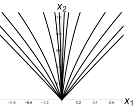
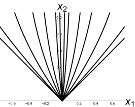
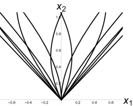
Figure 7: Projections of goedesics to the plane $(x_{1},x_{2})$ for $\lambda\in C_{4}$ (2 types) and $\lambda\in C_{6}$ (spacelike case)

In other cases the Hamiltonian system is easy to integrate. If $\lambda\in C_{5}$, then

$$x_{1}(t)\equiv 0,\quad x_{2}(t)=t,\quad y\equiv 0,\quad z=\frac{t^{3}}{6}.$$ (92)

Projection of the extremal to the plane $(x_{1},x_{2})$ is the vertical straight line. This case has no upper bounds for the time: $t_{\operatorname{supr}}=+\infty$.

If $\lambda\in C_{6}$, then

$$\alpha=0,\qquad c\equiv\operatorname{const}\nolimits\neq 0,\quad\theta=\theta_{0}-ct,$$

$$x_{1}(t) =\frac{\cosh(ct-\theta_{0})-\cosh\theta_{0}}{c},$$ (93)

$$x_{2}(t) =\frac{\sinh(ct-\theta_{0})+\sinh\theta_{0}}{c},$$ (94)

$$y(t) =\frac{ct-\sinh(ct)}{2c^{2}},$$ (95)

$$z(t) =\frac{4\cosh\big{(}\frac{3ct}{2}-3\theta_{0}\big{)}\sinh^{3}\frac{ct}{2}-3\cosh\theta_{0}\big{(}ct-\sinh(ct)\big{)}}{6c^{3}}.$$ (96)

Projections of extremals to the plane $(x_{1},x_{2})$ with $|\alpha|=1$ and $\psi_{0}=0$ (hyperbolas) are shown in Fig. 7, right. This case has no upper bounds for time: $t_{\operatorname{supr}}=+\infty$.

If $\lambda\in C_{7}$, then

$$\alpha=0,\qquad c\equiv 0,\quad\theta\equiv\operatorname{const}\nolimits,\quad\sinh\theta=s_{0},\quad\cosh\theta=c_{0},$$

$$x_{1}(t) =-s_{0}t,$$ (97)

$$x_{2}(t) =c_{0}t,$$ (98)

$$y(t) \equiv 0,$$ (99)

$$z(t) =\frac{c_{0}(1+2s_{0}^{2})}{6}t$$ (100)

Projections of extremals to the plane $(x_{1},x_{2})$ are straight lines. This case also has no upper bounds for time: $t_{\operatorname{supr}}=+\infty$.

So we obtained parameterization of the exponential mapping

$$\operatorname{Exp}\nolimits:N\to M={\mathbb{R}}^{4},\quad\operatorname{Exp}\nolimits(\lambda,t)=q(t),$$ (101)

$$N=\{(\lambda,t)\in C\times{\mathbb{R}}_{+}\leavevmode\nobreak\ |\leavevmode\nobreak\ t\in\big{(}0,t_{\operatorname{supr}}(\lambda)\big{)}\},$$ (102)

in the spacelike case. It maps a pair $(\lambda,t)$ to the point of corresponding extremal $q(t)$.

Further we investigate discrete symmetries of the exponential mapping and on this basis find estimates for the cut time on extremals.

6.2 Discrete symmetries of exponential mapping

Subsystem (67)-(69) for the costate variables of the normal Hamiltonian system has symmetries which preserve the direction field of this system.

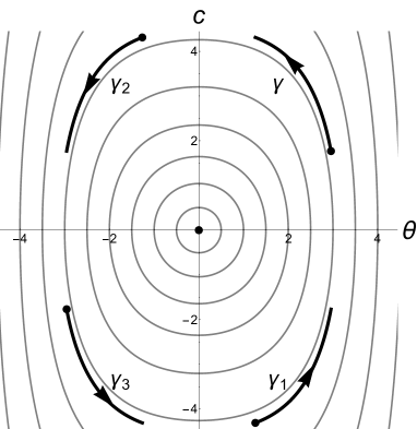
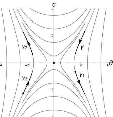
Figure 8: Action of symmetries on trajectories of vertical subsystem for $\alpha=-1,1$ (spacelike case)

Let us describe the action of symmetries $\varepsilon^{i}$ on the set of trajectories of the vertical subsystem with preservation of time direction. Denote a smooth curve

$$\gamma=\Big{\{}\big{(}\theta(t),c(t),\alpha\big{)}\leavevmode\nobreak\ |\leavevmode\nobreak\ t\in[0,T]\Big{\}}\subset C.$$

Define action of symmetries on these curves (see. Fig. 8):

$$\varepsilon^{1}:\gamma\mapsto\gamma_{1}=\Big{\{}\big{(}\theta^{1}(t),c^{1}(t),\alpha^{1}\big{)}\leavevmode\nobreak\ |\leavevmode\nobreak\ t\in[0,T]\Big{\}}=\Big{\{}\big{(}\theta(T-t),-c(T-t),\alpha\big{)}\Big{\}},$$

$$\varepsilon^{2}:\gamma\mapsto\gamma_{2}=\Big{\{}\big{(}\theta^{2}(t),c^{2}(t),\alpha^{2}\big{)}\leavevmode\nobreak\ |\leavevmode\nobreak\ t\in[0,T]\Big{\}}=\Big{\{}\big{(}-\theta(T-t),c(T-t),\alpha\big{)}\Big{\}},$$

$$\varepsilon^{3}:\gamma\mapsto\gamma_{3}=\Big{\{}\big{(}\theta^{3}(t),c^{3}(t),\alpha^{3}\big{)}\leavevmode\nobreak\ |\leavevmode\nobreak\ t\in[0,T]\Big{\}}=\Big{\{}\big{(}-\theta(t),-c(t),\alpha\big{)}\Big{\}}.$$

It is obvious that if $\gamma$ is a solution to the vertical subsystem (67)-(69), then $\gamma_{i},i=1,2,3,$ is a solution as well.

Consider the group of symmetries $G=\{\mathrm{Id},\varepsilon^{1},\varepsilon^{2},\varepsilon^{3}=\varepsilon^{1}\circ\varepsilon^{2}\}\cong{\mathbb{Z}}^{2}\times{\mathbb{Z}}^{2}$. The symmetry $\varepsilon^{3}$ preserves direction of time, while $\varepsilon^{1}$ and $\varepsilon^{2}$ change it.

Continue the action of symmetries from the vertical subsystem to solutions of the Hamiltonian system of PMP

$$\dot{\theta}(t)=-c(t),\quad\dot{c}(t)=-\alpha\sinh\theta(t),\quad\dot{\alpha}=0,$$

$$\dot{q}(t)=-\cosh\theta(t)X_{1}\big{(}q(t)\big{)}+\sinh\theta(t)X_{2}\big{(}q(t)\big{)},$$

in the following way:

$$\varepsilon^{i}:\Big{\{}\big{(}\theta(t),c(t),\alpha,q(t)\big{)}\leavevmode\nobreak\ |\leavevmode\nobreak\ t\in[0,T]\Big{\}}\mapsto\Big{\{}\big{(}\theta^{i}(t),c^{i}(t),\alpha^{i},q^{i}(t)\big{)}|t\in[0,T]\Big{\}}.$$ (103)

Let $q(t)=\big{(}x_{1}(t),x_{2}(t),y(t),z(t)\big{)},\ t\in[0,T],$ be a geodesic and

$$q^{i}(t)=\big{(}x_{1}^{i}(t),x_{2}^{i}(t),y^{i}(t),z^{i}(t)\big{)},\qquad t\in[0,T],\ i=1,2,3,$$

be its image under the action of a symmetry $\varepsilon^{i}$.

Lemma 7.

The symmetries $\varepsilon^{i}$ map trajectories in the plane $(x_{1},x_{2})$ in the following way:

$$x_{1}^{1}(t)=x_{1}(T)-x_{1}(T-t),\qquad x_{2}^{1}(t)=x_{2}(T)-x_{2}(T-t),$$

$$x_{1}^{2}(t)=x_{1}(T-t)-x_{1}(T),\qquad x_{2}^{2}(t)=x_{2}(T)-x_{2}(T-t),$$

$$x_{1}^{3}(t)=-x_{1}(t),\qquad x_{2}^{3}(t)=x_{2}(t).$$

Proof.

Using direct integration, for instance, for $\varepsilon^{1}$ we verify that

$$x_{1}^{1}(t)=\int_{0}^{t}\big{(}-\sinh\theta(T-s)\big{)}ds=-\int_{T-t}^{T}\big{(}-\sinh\theta(r)\big{)}dr=x_{1}(T)-x_{1}(T-t),$$

$$x_{2}^{1}(t)=\int_{0}^{t}\cosh\theta(T-s)ds=-\int_{T-t}^{T}\cosh\theta(r)dr=x_{2}(T)-x_{2}(T-t).$$

∎

Lemma 8.

The symmetries $\varepsilon^{i}$ maps endpoints of geodesics $q=\big{(}x_{1},x_{2},y,z\big{)}$ to endpoints of $q^{i}=\big{(}x_{1}^{i},x_{2}^{i},y^{i},z^{i}\big{)}$ in the following way:

$$x_{1}^{1}(T)=x_{1}(T), x_{2}^{1}(T)=x_{2}(T), y^{1}(T)=-y(T), z^{1}(T)=z(T)-x_{1}(T)y(T),$$

$$x_{1}^{2}(T)=-x_{1}(T), x_{2}^{2}(T)=x_{2}(T), y^{2}(T)=y(T), z^{2}(T)=z(T)-x_{1}(T)y(T),$$

$$x_{1}^{3}(T)=-x_{1}(T), x_{2}^{3}(T)=x_{2}(T), y^{3}(T)=-y(T), z^{3}(T)=z(T).$$

Proof.

Lemma 7 gives us expressions for $x_{1}^{i}(T)$ and $x_{2}^{i}(T)$. The expressions for other variables are obtained by integration. For example, for $\varepsilon^{1}$ we have

$$y^{1}(T) =\int_{0}^{T}\frac{x_{2}^{1}(t)\sinh\theta^{1}(t)+x_{1}^{1}(t)\cosh\theta^{1}(t)}{2}dt=\frac{x_{2}(T)}{2}\int_{0}^{T}\sin\theta(T-t)dt$$

$$\qquad+\frac{x_{1}(T)}{2}\int_{0}^{T}\cosh\theta(T-t)dt-\int_{0}^{T}\frac{x_{2}(s)\sinh\theta(s)+x_{1}(s)\cosh\theta(s)}{2}ds$$

$$=-\frac{x_{2}(T)x_{1}(T)}{2}+\frac{x_{1}(T)x_{2}(T)}{2}-y(T)=-y(T),$$

$$z^{1}(T) =\int_{0}^{T}\frac{\big{(}x_{1}^{1}(t)\big{)}^{2}+\big{(}x_{2}^{1}(t)\big{)}^{2}}{2}\dot{x}_{2}^{1}(t)dt=\frac{\big{(}x_{2}^{1}(T)\big{)}^{3}}{6}+\int_{0}^{T}\frac{\big{(}x_{1}^{1}(t)\big{)}^{2}}{2}\dot{x}_{2}^{1}(t)dt$$

$$=\frac{\big{(}x_{2}(T)\big{)}^{3}}{2}+\int_{0}^{T}\frac{\big{(}x_{1}(T)\big{)}^{2}-2x_{1}(T)x_{1}(T-t)+\big{(}x_{1}(T-t)\big{)}^{2}}{2}\dot{x}_{2}(T-t)dt$$

$$=\frac{\big{(}x_{2}(T)\big{)}^{3}}{6}+\frac{\big{(}x_{1}(T)\big{)}^{2}x_{2}(T)}{2}-x_{1}(T)\int_{0}^{T}x_{1}(s)\dot{x}_{2}(s)ds+z(T)-\frac{\big{(}x_{2}(T)\big{)}^{3}}{6}$$

$$=\frac{\big{(}x_{1}(T)\big{)}^{2}x_{2}(T)}{2}-x_{1}(T)\Big{(}y(T)+\frac{x_{1}(T)x_{2}(T)}{2}\Big{)}+z(T)=z(T)-x_{1}(T)y(T).$$

∎

We define the action of $\varepsilon^{i}$ in the preimage of exponential mapping $N$ by restricting action to the initial point of trajectory of the vertical subsystem:

$$\varepsilon^{i}:C\to C,\qquad\varepsilon^{i}(\theta,c,\alpha)=(\theta^{i},c^{i},\alpha^{i}),$$ (104)

$$(\theta^{1},c^{1},\alpha^{1})=(\theta,-c,-\alpha),$$ (105)

$$(\theta^{2},c^{2},\alpha^{2})=(-\theta,c,\alpha),$$ (106)

$$(\theta^{3},c^{3},\alpha^{3})=(-\theta,-c,-\alpha),$$ (107)

in the following way:

$$\varepsilon^{i}(\lambda,t)=\big{(}\varepsilon^{i}\circ e^{t\vec{H}_{v}}(\lambda),t\big{)},\qquad i=1,2,$$

$$\varepsilon^{3}(\lambda,t)=\big{(}\varepsilon^{3}(\lambda),t\big{)},$$

where $\vec{H}_{v}=-c\frac{\partial}{\partial\theta}-\alpha\sinh\theta\frac{\partial}{\partial c}\in\mathrm{Vec}(C)$ is the vertical part of the Hamiltonian vector field.

We define the action of $\varepsilon^{i}$ in the image $M$ of the exponential mapping $M$ by restricting the action to endpoints of geodesics (see Lemma 8):

$$\varepsilon^{i}:M\to M,\quad\varepsilon^{i}(q)=\varepsilon^{i}(x_{1},x_{2},y,z)=q^{i}=(x_{1}^{i},x_{2}^{i},y^{i},z^{i}),$$ (108)

$$(x_{1}^{1},x_{2}^{1},y^{1},z^{1})=(x_{1},\ x_{2},\ -y,\ z-x_{1}y),$$ (109)

$$(x_{1}^{2},x_{2}^{2},y^{2},z^{2})=(-x_{1},\ x_{2},\ y,\ z-x_{1}y),$$ (110)

$$(x_{1}^{3},x_{2}^{3},y^{3},z^{3})=(-x_{1},\ x_{2},\ -y,\ z).$$ (111)

Since the actions of $\varepsilon^{i}$ in the domain $N$ and the image $M$ of the exponential map are induced by the actions of symmetries (103) on trajectories of Hamiltonian system, we have the following result.

Proposition 2.

The mappings $\varepsilon^{i},i=1,2,3,$ are symmetries of the exponential mapping, i.e.,

$$(\varepsilon^{i}\circ\operatorname{Exp}\nolimits)(\theta,c,\alpha,t)=(\operatorname{Exp}\nolimits\circ\varepsilon^{i})(\theta,c,\alpha,t),\qquad(\theta,c,\alpha,t)\in N.$$

6.3 Maxwell points of spacelike normal extremals

In this section we compute the Maxwell points corresponding to the symmetries $\varepsilon^{i}$. On this basis we derive estimates for the cut time along extremals.

We define the Maxwell sets in the preimage of $\operatorname{Exp}\nolimits$ corresponding to the symmetries $\varepsilon^{i}$:

$$\operatorname{MAX}\nolimits^{i}=\big{\{}(\lambda,t)\in N\leavevmode\nobreak\ |\leavevmode\nobreak\ \lambda^{i}\neq\lambda,\ \operatorname{Exp}\nolimits(\lambda^{i},t)=\operatorname{Exp}\nolimits(\lambda,t)\big{\}},\quad\lambda=(\theta,c,\alpha),\ \lambda^{i}=\varepsilon^{i}(\lambda).$$

It follows from Proposition 2 that the equality $\operatorname{Exp}\nolimits(\lambda^{i},t)=\operatorname{Exp}\nolimits(\lambda,t)$ is equivalent to $\varepsilon^{i}\big{(}q(t)\big{)}=q(t)$. Therefore we get a description of fixed points of the symmetries $\varepsilon^{i}$ in the preimage of the exponential mapping.

Lemma 9.

1. $\varepsilon^{1}(q)=q\leavevmode\nobreak\ \Longleftrightarrow\leavevmode\nobreak\ y=0$.

2. $\varepsilon^{2}(q)=q\leavevmode\nobreak\ \Longleftrightarrow\leavevmode\nobreak\ x_{1}=0$.

3. $\varepsilon^{3}(q)=q\leavevmode\nobreak\ \Longleftrightarrow\leavevmode\nobreak\ x_{1}^{2}+y^{2}=0$.

Proof.

Follows from definition (108)–(111) of action of the symmetries in $M$. ∎

Now we compute fixed points of symmetries in the preimage of the exponential mapping, which is necessary for description of Maxwell sets. Introduce the following coordinates in the set $\cup_{i=1}^{3}N_{i},\ N_{i}=\{(\lambda,t)\in C_{i}\times{\mathbb{R}}_{+}\leavevmode\nobreak\ |\leavevmode\nobreak\ t\in\big{(}0,t_{\operatorname{supr}}(\lambda)\big{)}\}$:

$$\tau=\frac{\psi_{t}+\psi_{0}}{2},\qquad p=\frac{\psi_{t}-\psi_{0}}{2}=\frac{\ae t}{2}.$$ (112)

The parameter $\tau$ corresponds to the middle point of a trajectory.

Lemma 10.

1. $\lambda^{1}=\lambda\leavevmode\nobreak\ \Longleftrightarrow\leavevmode\nobreak\ \left\{\begin{array}[]{l}\operatorname{sn}\nolimits\tau=0,\text{ if }\lambda\in C_{1}\cup C_{2},\\ \text{impossible, if }\lambda\in C_{3}\cup C_{4}\cup C_{6},\\ c=0,\text{ if }\lambda\in C_{5}\cup C_{7}.\end{array}\right.$

2. $\lambda^{2}=\lambda\leavevmode\nobreak\ \Longleftrightarrow\leavevmode\nobreak\ \left\{\begin{array}[]{l}\operatorname{cn}\nolimits\tau=0,\text{ if }\lambda\in C_{1},\\ \text{impossible, if }\lambda\in C_{2}\cup C_{4},\\ \operatorname{sn}\nolimits\tau=0,\text{ if }\lambda\in C_{3},\\ \theta=0,\text{ if }\lambda\in\bigcup_{i=5}^{7}C_{i}.\end{array}\right.$

3. $\lambda^{3}=\lambda\leavevmode\nobreak\ \Longleftrightarrow\leavevmode\nobreak\ \left\{\begin{array}[]{l}\text{impossible, if }\lambda\in(\bigcup_{i=1}^{4}C_{i})\cup C_{6},\\ \theta=c=0\text{, if }\lambda\in C_{5}\cup C_{7}.\end{array}\right.$

Proof.

Follows from definition of action of the symmetries in the domain of the exponential mapping (104)–(107) and definition (112) of the coordinate $\tau$. ∎

The equations $\varepsilon^{i}(q)=q$ define sub-manifolds in ${\mathbb{R}}^{4}$ with dimension from 3 to 2, the exponential mapping transforms the corresponding Maxwell sets into these sub-manifolds:

$$\operatorname{Exp}\nolimits(\operatorname{MAX}\nolimits^{i})\subset\{q\in{\mathbb{R}}^{4}\leavevmode\nobreak\ |\leavevmode\nobreak\ \varepsilon^{i}(q)=q\}\quad i=1,2,3.$$

Further we describe in detail the sets $\operatorname{MAX}\nolimits^{1},\operatorname{MAX}\nolimits^{2}$ since they define sub-manifolds in $M$ with the maximum dimension 3, while $\operatorname{MAX}\nolimits^{3}$ defines a sub-manifold with dimension 2. We investigate roots of the equations $x_{1}=0,y=0$ along a geodesic. Using coordinates (112) for the case $\lambda\in C_{1}$ we get

$$x_{1} =\frac{2\sqrt{2(\alpha+E)}\operatorname{cn}\nolimits\tau\operatorname{dn}\nolimits\tau\operatorname{sn}\nolimits p}{\alpha(1-k^{2}\operatorname{sn}\nolimits^{2}p\operatorname{sn}\nolimits^{2}\tau)},$$

$$y =\frac{2\sqrt{2(\alpha+E)}\operatorname{sn}\nolimits\tau f_{1}(p)}{\alpha^{2}\ae(1-k^{2}\operatorname{sn}\nolimits^{2}p\operatorname{sn}\nolimits^{2}\tau)},$$

$$f_{1}(p) =\alpha p\operatorname{cn}\nolimits p\operatorname{dn}\nolimits p+\ae^{2}\big{(}2\operatorname{cn}\nolimits p\operatorname{dn}\nolimits p\operatorname{E}\nolimits(p)-(1+k^{2})\operatorname{sn}\nolimits p+2k^{2}\operatorname{sn}\nolimits^{3}p\big{)}.$$

This gives us description of the Maxwell sets in $N$:

$$\operatorname{MAX}\nolimits^{1}\cap N_{1} =\{\nu\in N_{1}\mid y=0,\operatorname{sn}\nolimits\tau\neq 0\}=\{\nu\in N_{1}\mid f_{1}(p)=0\},$$ (113)

$$\operatorname{MAX}\nolimits^{2}\cap N_{1} =\{\nu\in N_{1}\mid x_{1}=0,\operatorname{cn}\nolimits\tau\neq 0\}=\{\nu\in N_{1}\mid\operatorname{sn}\nolimits p=0\},$$ (114)

where $\nu=(\tau,p,E,\alpha)$.

Let $p_{1}^{i},i\in{\mathbb{N}}$, denote a positive root of equation $f_{1}(p)=0$, s.t. $p_{1}^{1}<p_{1}^{2}<\dots<p_{1}^{i}<\cdots$. We have $t_{\operatorname{MAX}\nolimits^{1}}(\lambda)=p_{1}^{1}$, $t_{\operatorname{MAX}\nolimits^{2}}(\lambda)=2\operatorname{K}\nolimits$. There is a conjecture (this conjecture is supported numerically) that $t_{\operatorname{MAX}\nolimits^{2}}(\lambda)<t_{\operatorname{MAX}\nolimits^{1}}(\lambda)$. This means that each geodesic from $C_{1}$ meets the set $\operatorname{MAX}\nolimits^{2}$ first.

If $\lambda\in C_{2}$, then

$$x_{1} =-\frac{2\operatorname{sgn}\nolimits\theta\sqrt{2}\sqrt{-\alpha-E}\operatorname{dn}\nolimits\tau\operatorname{cn}\nolimits p\operatorname{sn}\nolimits p}{\alpha(\operatorname{cn}\nolimits^{2}\tau-\operatorname{sn}\nolimits^{2}p\operatorname{dn}\nolimits^{2}\tau)},$$

$$y =\frac{2\operatorname{sgn}\nolimits\theta\sqrt{2}\sqrt{-\alpha-E}\operatorname{cn}\nolimits\tau\operatorname{sn}\nolimits\tau f_{2}(p)}{\alpha^{2}\ae(\operatorname{cn}\nolimits^{2}\tau-\operatorname{sn}\nolimits^{2}p\operatorname{dn}\nolimits^{2}\tau)},$$

$$f_{2}(p) =-E(p)\operatorname{dn}\nolimits p-\ae^{2}\big{(}2\operatorname{dn}\nolimits p\operatorname{E}\nolimits(p)-k^{2}\operatorname{cn}\nolimits p\operatorname{sn}\nolimits p\big{)}$$ (115)

We have

$$\operatorname{MAX}\nolimits^{1}\cap N_{2} =\{\nu\in N_{2}\mid y=0,\operatorname{sn}\nolimits\tau\neq 0,\tau\in(-\operatorname{K}\nolimits,\operatorname{K}\nolimits),p\in(0,\operatorname{K}\nolimits)\}$$

$$\subset\{\nu\in N_{2}\mid f_{2}(p)=0,p\in(0,\operatorname{K}\nolimits)\},$$ (116)

$$\operatorname{MAX}\nolimits^{2}\cap N_{2} =\{\nu\in N_{2}\mid x_{1}=0,\tau\in(-\operatorname{K}\nolimits,\operatorname{K}\nolimits),p\in(0,\operatorname{K}\nolimits)\}=\emptyset,$$ (117)

where $\nu=(\tau,p,E,\alpha)$.

Lemma 11.

The function $f_{2}(p)>0$ for $p\in\big{(}0,\operatorname{K}\nolimits(k)\big{)},k\in(0,1)$.

Proof.

We show that $g(p)=\operatorname{dn}\nolimits p$ is a comparison function for $f_{2}(p)$ for $p\in(0,\operatorname{K}\nolimits)$.

The inequality $f_{2}(p)\not\equiv 0$ follows from the expansion $f_{2}(p)=\frac{1}{3}\alpha k^{2}p^{3}+o(p^{3})$. Notice that $g(p)>0$ for $p\in(0,\operatorname{K}\nolimits)$. Finally we get the equalities

$$\bigg{(}\frac{f_{2}(p)}{g(p)}\bigg{)}^{\prime}=\frac{\alpha^{2}\operatorname{sn}\nolimits^{2}p\operatorname{cn}\nolimits^{2}p}{\ae^{2}\operatorname{dn}\nolimits^{2}p},\qquad\frac{f_{2}(p)}{g(p)}=\frac{1}{3}\alpha k^{2}p^{3}+o(p^{3}).$$

So $g(p)$ is a comparison function for $f_{2}(p)$; thus, it follows from Lemma 5 that $f_{2}(p)>0$ for $p\in(0,\operatorname{K}\nolimits)$. ∎

Proposition 3.

$\operatorname{MAX}\nolimits^{1}\cap N_{2}=\emptyset$.

Proof.

Follows immediately from Lemma 11 and (116). ∎

If $\lambda\in C_{3}$, then

$$x_{1} =\frac{4\operatorname{sgn}\nolimits c\operatorname{sn}\nolimits p\operatorname{sn}\nolimits\tau}{\ae(\operatorname{cn}\nolimits^{2}\tau-\operatorname{dn}\nolimits^{2}\tau\operatorname{sn}\nolimits^{2}p)},$$

$$y =-\frac{4\operatorname{sgn}\nolimits c\operatorname{cn}\nolimits\tau\operatorname{dn}\nolimits\tau f_{3}(p)}{\ae^{2}(1-k_{2})^{2}(\operatorname{cn}\nolimits^{2}\tau-\operatorname{dn}\nolimits^{2}\tau\operatorname{sn}\nolimits^{2}p)},$$

$$f_{3}(p) =\operatorname{cn}\nolimits p\operatorname{dn}\nolimits p\big{(}(1-k_{2})p-2\operatorname{E}\nolimits(p)\big{)}+(1+k_{2})\operatorname{sn}\nolimits p-2k_{2}\operatorname{sn}\nolimits^{3}p.$$ (118)

We have

$$\operatorname{MAX}\nolimits^{1}\cap N_{3} =\{\nu\in N_{3}\mid y=0,\tau\in(-\operatorname{K}\nolimits,\operatorname{K}\nolimits),p\in(0,\operatorname{K}\nolimits)\}$$

$$=\{\nu\in N_{3}\mid f_{3}(p)=0,p\in(0,\operatorname{K}\nolimits)\},$$ (119)

$$\operatorname{MAX}\nolimits^{2}\cap N_{3} =\{\nu\in N_{3}\mid x_{1}=0,\operatorname{sn}\nolimits\tau\neq 0,\tau\in(-\operatorname{K}\nolimits,\operatorname{K}\nolimits),p\in(0,\operatorname{K}\nolimits)\}=\emptyset,$$

where $\nu=(\tau,p,E,\alpha)$.

Lemma 12.

The function $f_{3}(p)>0$ for $p\in(0,\operatorname{K}\nolimits)$.

Proof.

We show that $g(p)=\operatorname{cn}\nolimits p\operatorname{dn}\nolimits p$ is a comparison function for $f_{3}(p)$ for $p\in(0,\operatorname{K}\nolimits)$.

The inequality $f_{3}(p)\not\equiv 0$ follows from the expansion $\displaystyle f_{3}(p)=\frac{\alpha^{2}}{3\ae^{4}}p^{3}+o(p^{3})$. Notice that $g(p)>0$ for $p\in(0,\operatorname{K}\nolimits)$. Finally we get the equalities

$$\bigg{(}\frac{f_{3}(p)}{g(p)}\bigg{)}^{\prime}=\frac{(1-k_{2})^{2}\operatorname{sn}\nolimits^{2}p}{\operatorname{cn}\nolimits^{2}p\operatorname{dn}\nolimits^{2}p},\qquad\frac{f_{2}(p)}{g(p)}=\frac{\alpha^{2}}{3\ae^{4}}p^{3}+o(p^{3}).$$

So $g(p)$ is a comparison function for $f_{3}(p)$; thus, it follows from Lemma 5 that $f_{3}(p)>0$ for $p\in(0,\operatorname{K}\nolimits)$. ∎

Remark 3.

Notice that if $k^{2}=k_{2}<0$, then Lemma 12 is valid. We have the following formulas:

$$x_{1} =\frac{2\sqrt{2}\sqrt{\alpha+E}\operatorname{sgn}\nolimits c\operatorname{dn}\nolimits\tau\operatorname{sn}\nolimits\tau\operatorname{dn}\nolimits p\operatorname{sn}\nolimits p}{\alpha(\operatorname{cn}\nolimits^{2}\tau-\operatorname{dn}\nolimits^{2}\tau\operatorname{sn}\nolimits^{2}p)},$$

$$y =\frac{2\sqrt{2}\operatorname{cn}\nolimits\tau\sqrt{\alpha+E}\operatorname{sgn}\nolimits cf_{4}(p)}{\alpha\ae(\operatorname{cn}\nolimits^{2}\tau-\operatorname{dn}\nolimits^{2}\tau\operatorname{sn}\nolimits^{2}p)},\qquad\ae=\hat{\ae}=\sqrt{\alpha},$$

$$f_{4}(p) =2\operatorname{cn}\nolimits p\operatorname{E}\nolimits(p)-p\operatorname{cn}\nolimits p-\operatorname{dn}\nolimits p\operatorname{sn}\nolimits p,\qquad k=\hat{k}=\sqrt{\frac{\alpha-E}{2\alpha}}.$$

One can easily prove that $g(p)=\operatorname{cn}\nolimits p$ is a comparison function for $f_{4}(p)$ for $p\in(0,\operatorname{K}\nolimits)$.

Proposition 4.

$\operatorname{MAX}\nolimits^{1}\cap N_{3}=\emptyset$.

Proof.

Follows immediately from Lemma 12 and (119). ∎

We found the following upper bound for the cut time along general extremal with $\lambda\in\bigcup_{i=1}^{3}C_{i}$:

Theorem 6.

$$\lambda\in C_{1}\leavevmode\nobreak\ \Longrightarrow\leavevmode\nobreak\ t_{\operatorname{cut}}(\lambda)\leq 2\operatorname{K}\nolimits(k).$$ (120)

$$\lambda\in C_{2}\cup C_{3}\leavevmode\nobreak\ \Longrightarrow\leavevmode\nobreak\ t_{\operatorname{cut}}(\lambda)\leq\frac{\operatorname{K}\nolimits(k)-\psi_{0}}{\ae}.$$ (121)

There is a conjecture that this bound is sharp.

7 Conclusion

In this paper we consider extremals in the Engel group with a sub-Lorentzian metric. For this problem

$\bullet$ we prove that timelike normal extremals are locally maximizing;

$\bullet$ we calculate the timelike, spacelike and lightlike normal extremal trajectories;

$\bullet$ we describe the symmetries of the exponential map and the corresponding Maxwell points of timelike, spacelike normal extremals;

$\bullet$ we obtain an upper estimate for the cut time on extremal trajectories.

In the future we are intending to investigate the optimality of extremal trajectories, relying on the method of nonlinear approximation we shall also apply our results to consider general non-linear systems with 2-dimensional control in a 4-dimensional space with a sub-Lorentzian metric.

References

- [1] A.A. Agrachev, El-H. Chakir El-A.,and J. P. Gauthier, Sub-Riemannian metrics on , Proc. Conf. Canad. Math. Soc. 25(1998).
- [2] A. Agrachev, D. Barilari, and U. Boscain, On the Hausdorff volume in sub-Riemannian geometry, Calculus of Variations and Partial Differential Equations 10.1007/s00526-011-0414-y (2011), 1–34.
- [3] A. Agrachev, U. Boscain, J.-P. Gauthier, and F. Rossi, The intrinsic hypoelliptic Laplacian and its heat kernel on unimodular Lie groups, J. Funct. Anal. 256(2009), No. 8, 2621–2655.
- [4] A. A. Agrachev, G. Charlot, J. P. A. Gauthier, and V. M. Zakalyukin, On sub-Riemannian caustics and wave fronts for contact distributions in the three-space, J. Dynam. Control Systems 6 (2000), No. 3, 365-395.
- [5] A. Ardentov, Yu. Sachkov, Extremal trajectories in a nilponent sub-Riemannian problem on the Engel group, Matematicheskii Sbornik 202(2011), No. 11, 31-54.
- [6] A. Ardentov, Yu. Sachkov, Conjugate points in nilpotent sub-Riemannian problem on the Engel group, J. Mathematical Sciences 195(2013), No. 3, 369-390.
- [7] A. Ardentov, Yu. Sachkov, Cut time in sub-Riemannian problem on Engel group, ESAIM: Control, Optimisation and Calculus of Variations, accepted (2015)
- [8] N. I. Akhiezer. Elements of the theory of elliptic functions. Providence, RI: American Mathematical Society. 1990.
- [9] Cartan, , Sur quelques quadratures clout l’elernent diflerentiel contient des fonctions arbitraires, Bull. Soc. Math. France 29(1901), 118-130.
- [10] Q. Cai, T. Huang, Yu. Sachkov, X. Yang, in the Engel group with a sub-Lorentzian metric, submitted.
- [11] El-H. Alaoui, J-P. Gauthier, and I. Kupka, Small sub-Riemannian balls in , J. Dynam. Control Sys. 2(1996), No. 3, 359-421.
- [12] R. Beals, B. Gaveau, and P.C. Greiner, Hamilton-Jacobi theory and the Heat Kernal on Heisenberg groups, J. Math. Pures Appl. 79,7(2000) 633-689.
- [13] J.K. Beem, P.E. Ehrlich, and K.l. Easley, Global Lorentzian geometry, Marcel Dekker(1996).
- [14] D. C. Chang, I. Markina, and A. Vasiliev, Sub-Lorentzian geometry on anti-De Sitter space, J. Math. Pures Appl. 90(2008), No. 1, 82-110.
- [15] M. Golubitsky and V. Guillemin, Stable mappings and their singularities, Spinger-Verlag, New York(1973).
- [16] M. Grochowski, Differential properties of the sub-Riemannian distance function, Bull. Polish. Acad. Sci. 50(2002), No. 1.
- [17] M. Grochowski, Geodesics in the sub-Lorentzian geometry, Bull. Polish. Acad. Sci. 50(2002), No. 2, 162-178.
- [18] M. Grochowski, Normal forms of germs of Contact sub-Lorentzian structures on , Differentiability of the sub-Lorentzian distance function, J. Dynam. Control Sys. 9(2003), No. 4, 531-547.
- [19] M. Grochowski, Reachable sets for the Heisenberg sub-Lorentzian structure on , an estimate for the distance function, J. Dynam. Control Sys. 12(2006), No. 2, 145-160.
- [20] M. Grochowski, On the Heisenberg sub- Lorentzian Metric on , Geometric Singularity Theory, Banach Center Publications, 65(2004), 57-65.
- [21] M. Gromov, Carnot-Caratheodory spaces seen from within, Progr. Math. 144, Birkhauser, Boston (1996), 79-323.
- [22] T. Huang, X. Yang, Geodesics in the Heisenberg Group with a Lorentzian metric, J. Dynam. Control Sys. 18(2012), No. 1, 21-40.
- [23] F. Monroy-Prez, and A. Anzaldo-Meneses, Optimal control on the Heisenberg group, J. Dynam. Control Sys. 5(1996), No.4, 473-499.
- [24] B. O’Neill, Semi-Riemannian Geometry: with Applications to Relativity, Pure and Applied Mathematics, vol. 103, Academic Press, Inc., New York, 1983.
- [25] A. Korolko, and I. Markina, Non-holonomic Lorentzian geometry on some -type groups, J. Geom. Anal. 19(2009), 864-889.
- [26] R. Montgomery, Singular extremals on Lie groups, Math. Control, Signals and Systems vol. 7(3) (1994), 217-234.
- [27] R. Montgomery, A tour of sub-Riemannian geometries, their geodesics and applications, Math. Surveys and Monographs 91, American Math. Soc., Providence, 2002.
- [28] P. Piccione, and D.V. Tausk, Variational aspects of the geodesic problem in sub-Riemannian geometry, J. Geometry and Physics. 39(2001), 183-206.
- [29] Yu. L. Sachkov, Conjugate and cut time in the sub-Riemannian problem on the group of motions of a plane, ESAIM Control Optim. Calc. Var.16 (2010), 1018-1039.
- [30] R. Strichartz, Sub-Riemannian geometry, J. Diff. Geom., 24(1986), 221-263.