Advantages of nonclassical pointer states in postselected weak measurements

Abstract

We investigate, within the weak measurement theory, the advantages of non-classical pointer states over semi-classical ones for coherent, squeezed vacuum, and Schröinger cat states. These states are utilized as pointer state for the system operator $\hat{A}$ with property $\hat{A}^{2}=\hat{I}$, where $\hat{I}$ represents the identity operator. We calculate the ratio between the signal-to-noise ratio (SNR) of non-postselected and postselected weak measurements. The latter is used to find the quantum Fisher information for the above pointer states. The average shifts for those pointer states with arbitrary interaction strength are investigated in detail. One key result is that we find the postselected weak measurement scheme for non-classical pointer states to be superior to semi-classical ones. This can improve the precision of measurement process.

I Introduction

The weak measurement, as a generalized von Neumann quantum measurement theory, was proposed by Aharonov, Albert, and VaidmanAharonov(1988) . In weak measurement, the coupling between pointer and measured systems is sufficiently weak, but its induced weak value of the observable on the measured system can be beyond the usual range of the eigenvalues of that observableqparadox(2005) . This feature of weak value is usually referred to as an amplification effect for weak signals rather than a conventional quantum measurement that collapses a coherent superposition of quantum statesAharonov(1988) ; Tollaksen(2010) .

After first optical implementation of weak valueRitchie(1991) , it has been applied in different fields to observe very tiny effects, such as beam deflection Pfeifer(2011) ; Hosten2008 ; Hogan(2011) ; Zhou(2013) ; Starling(2009) ; Dixon(2009) , frequency shifts Starling(2010)-1 , phase shifts Starling(2010) , angular shifts Magana(2013) ; Bertulio (2014) , velocity shifts viza(2013) , and even temperature shift Egan(2012) . Weak value has a nature of being a complex number, which lead the weak measurements to provide an ideal method to examine some fundamentals of quantum physics. Quantum paradoxes (Hardy’s paradox Aharonov(2002) ; Lundeen(2009) ; Yokota (2009) and the three-box paradox Resch(2004) ), quantum correlation and quantum dynamics Aharonov(2005) ; Aharonov(2008) ; Holger(2013) ; Aharonov(2011) ; Shikano(2011) ; Shikano(2010) , quantum state tomography Lundeen (2011) ; Lundeen(2012) ; Braveman(2013) ; Kocsis(2011) ; Malik(2014) ; Salvail(2013) , violation of the generalized Leggett-Garg inequalities Palacios ; Suzuki(2012) ; Dressel (2011) ; Emary(2014) ; Goggin(2011) ; Groen(2013) and violation of the initial Heisenberg measurement-disturbance relationship Lee(2012) ; Eda(2014) are just few examples. In these typical examples, the small effects have been amplified due to the benefit of weak values. This amplifying effect occurs when the preselection and postselection states of the measured system are almost orthogonal. The successful postselection probability tends to decrease in order to have successful amplification effect. For more details about weak measurement and weak value, one can consult these reviews Dressel(2014) ; Nori ; Shikano(2012) .

So far, most of weak measurement studies focus on using the zero-mean Gaussian state as an initial pointer state. However, recent studies Wu ; Knee(2014) have shown that zero-mean Gaussian pointer state cannot improve the SNR when considering postselection probability. Needless to say Gaussian beam is classical and one may naturally ask how about using non-classical pointer states, and what kind of advantages they have? This issue has been recently addressed Pang(2014) , where coherent and coherent squeezed states were utilized as pointers. They showed that the postselected weak measurement improved the SNR compared to the non-postselected process if the pointer state, is non-classical rather than classical. The focus of the calculation was based on the assumption that the coupling between measuring device and measured system is too weak, and hence it was enough to consider the time evolution operator up to its first order. Furthermore, there have been recent studies giving full order effects of the unitary evolution due to the von Neumann interaction, but for classical and semi-classical statesTurek ; Nakamura(2012) .

In this paper, we address a remaining point of interest constructing a general formula for weak measurement beyond the first order, and utilizing the non-classical states. We investigate the advantages of non-classical pointer states over classical (semi-classical ) pointer state, within weak values, by considering postselection probability. In order to do so, we use coherent, squeezed vacuum, and Schröinger cat states as pointer states for system observable $\hat{A}$ with property $\hat{A}^{2}=\hat{I}$. We start by presenting an analytical general expressions of the shifted values of position and momentum operators for the above mentioned pointer states with arbitrary measurement strengths. In addition, we present the ratio of SNR between postselected and non-postselected weak measurement, and also look at quantum Fisher information. Our key results in this paper are (i) Our general expressions of shifted values reduce to the Nakamura’sNakamura(2012) main result if we take the zero-mean Gaussian beam as initial pointer state. (ii) As shown in Ref.Pang(2014) , improving the SNR using postselected weak measurement, one needs the non-classical pointer states which is better than classical or semi-classical states. (iii) Non-classical pointer states are much better even when it comes to parameter estimation process which is characterized by Fisher information.

The rest of the paper is organized as follows. In Section II, we give the setup for our system. In Section III, we start by giving general expressions for the expectation values of position and momentum operators. After that we discuss the ratio of SNR between postselected and non-postselected weak measurements of coherent, squeezed vacuum, and Schröinger cat states. In Section IV, we give the Fisher information for those given states in the light of postselection probability. We give conclusion to our paper in section V. Throughout this paper, we use the unit $\hbar=1$.

II Setup

For the weak measurement, the coupling interaction between system and measuring device is given by the standard von Neumann Hamiltonianqparadox(2005)

$$H=g\delta(t-t_{0})\hat{A}\otimes\hat{P}.$$ (1)

Here, $g$ is a coupling constant and $\hat{P}=\int p|p\rangle\langle p|dp$ is the conjugate momentum operator, while the position operator is $\hat{X}=\int x|x\rangle\langle x|dx$ where $[\hat{X},\hat{P}]=i\hat{I}$. We have taken, for simplicity, the interaction to be impulsive at time $t=t_{0}$. For this kind of impulsive interaction the time evolution operator becomes as $e^{-ig\hat{A}\otimes\hat{P}}$.

The weak measurement is characterized by the preselection and postselection of the system state. If we prepare the initial state $|\psi_{i}\rangle$ of the system and the pointer state, and after some interaction time $t_{0}$, we then postselect a system state $|\psi_{f}\rangle$ and obtain the information about a physical quantity $\hat{A}$ from the pointer wave function by the following weak value:

$$\langle A\rangle{}_{w}=\frac{\langle\psi_{f}|\hat{A}|\psi_{i}\rangle}{\langle\psi_{f}|\psi_{i}\rangle},$$ (2)

where the subscript $w$ denotes the weak value. From Eq. (2), we know that when the preselected state $|\psi_{i}\rangle$ and the postselected state $|\psi_{f}\rangle$ are almost orthogonal, the absolute value of the weak value can be arbitrarily large. This feature leads to weak value amplification.

We express position operator $\hat{X}$ and momentum operator $\hat{P}$ in terms of the annihilation (creation) operator, $\hat{a}$($\hat{a}^{\dagger}$) in Fock space representation as

$$\hat{X} = \sigma(\hat{a}^{\dagger}+\hat{a}),$$ (3)

$$\hat{P} = \frac{i}{2\sigma}(\hat{a}^{\dagger}-\hat{a}),$$ (4)

where $\sigma$ is the width of the fundamental Gaussian beam. These annihilation (creation) operators obey the commutation relation $[\hat{a},\hat{a}^{\dagger}]=\hat{I}$. By substituting Eq.(4) into unitary evolution operator $e^{-ig\hat{A}\otimes\hat{P}}$, bearing in mind that operator $\hat{A}$ satisfies the property $\hat{A}^{2}=\hat{I}$, we get:

$$e^{-ig\hat{A}\otimes\hat{P}}=\frac{1}{2}(\hat{I}+\hat{A})\otimes D(\frac{s}{2})+\frac{1}{2}(\hat{I}-\hat{A})\otimes D(-\frac{s}{2}),$$ (5)

where parameter $s$ is defined by $s:\equiv g/\sigma$, and $D\left(\mu\right)$ is a displacement operator with complex number $\mu$ defined by

$$D(\mu)=e^{\mu\hat{a}^{\dagger}-\mu^{\ast}\hat{a}}.$$ (6)

Note that $s$ characterizes the measurement strength. Thus, we can say that the coupling between system and pointer is weak (strong) and so the measurement is called weak (strong) measurement, if $s\ll 1$$(s\gg 1)$.

III The shifted values and the signal-to-noise ratio (SNR)

In this section we start by giving general shifted values of semi-classical state (coherent state) and non-classical states; squeezed vacuum and Schröinger cat pointer states for arbitrary measurement strength $s$. To show the advantages of non-classical pointer states over semi-classical ones, we discuss the ratio of SNR between postselected and non-postselected weak measurements

$$\mathcal{\chi=}\frac{R_{X}^{p}}{R_{X}^{n}}.$$ (7)

Here, $R_{X}^{p}$ represents the SNR of postselected weak measurement defined as

$$R_{X}^{p}=\frac{\sqrt{NP_{s}}|\langle X\rangle_{fi}|}{\sqrt{\langle X^{2}\rangle_{f}-\langle X\rangle_{f}^{2}}}.$$ (8)

Here, $N$ is the total number of measurements, $P_{s}$ is probability of finding the postselected state for a given preselected state, and $NP_{s}$ is the number of times the system was found in a postselected state. Here, $\langle\rangle_{f}$ denotes the expectation value of measuring observable under the final state of the pointer.

When dealing with non-postselected measurement, there is no postselection process after the interaction between system and measuring device due to unitary evolution operator $e^{-ig\hat{A}\otimes\hat{P}}$. Therefore, the definition of $R_{X}^{p}$ for non-postselected weak measurement can be given as

$$R_{X}^{n}=\frac{\sqrt{N}|\langle X\rangle_{f^{\prime}i}|}{\sqrt{\langle X^{2}\rangle_{f^{\prime}}-\langle X\rangle_{f^{\prime}}^{2}}}.$$ (9)

Here, $\langle\rangle_{f^{\prime}}$ denotes the expectation value of measuring observable under the final state of the pointer without postselection.

III.1 Coherent pointer state

Coherent state is typical semi-classical state which satisfies the minimum Heisenberg uncertainty relation. Here, we take the coherent state Scully as initial pointer state

$$\left|\alpha\right\rangle=D(\alpha)\left|0\right\rangle,$$ (10)

where $\alpha=re^{i\phi}$ is an arbitrary complex number. After unitary evolution given in Eq. (5), the resultant system state is postselected to $|\psi_{f}\rangle$. Then, we obtain the following normalized final pointer state:

$$|\Psi_{f_{1}}\rangle \!\!\!\!= \frac{\lambda}{2}\times$$

$$\!\!\!\!\!\![(1+\!\!\langle A\rangle_{w})e^{-i\frac{s}{2}\Im\left(\alpha\right)}|\alpha\!\!+\frac{s}{2}\rangle+(1-\!\!\langle A\rangle_{w})e^{i\frac{s}{2}\Im\left(\alpha\right)}|\alpha\!\!-\frac{s}{2}\rangle],$$

where the normalization coefficient is given as

$$\lambda = \sqrt{2}\times$$

$$[1\!+\!|\langle A\rangle_{w}|^{2}\!\!+\!\!\Re((1\!-\!\langle A\rangle{}_{w}^{\ast})(1\!\!+\!\!\langle A\rangle_{w})e^{-2is\Im\left(\alpha\right)})e^{-\frac{1}{2}s^{2}}]^{-\frac{1}{2}},$$

and $\Im$ ($\Re$) represents the imaginary (real) part of a complex number. Using Eqs.(III.1,III.1) we can calculate general forms of the expectation values of conjugate position operator $X$ and momentum operator $P$, under the final pointer state $|\Psi_{f_{1}}\rangle$, to be

$$\langle X\rangle_{f_{1}} = \sigma|\lambda|^{2}\{(1+|A{}_{w}|^{2})\Re(\alpha)+s\Re\langle A\rangle_{w}$$

$$\!\!\!\!+\Re[(1\!\!-\!\!\langle A\rangle_{w}^{\ast})(1\!\!+\!\!\langle A\rangle_{w})e^{-2si\Im(\alpha)}]\Re(\alpha)e^{-\frac{1}{2}s^{2}}\}$$

and

$$\langle P\rangle_{f_{1}} = \frac{|\lambda|^{2}}{4\sigma}\{2(1+|\langle A\rangle_{w}|^{2})\Im(\alpha)$$

$$\!\!\!\!-\Im[(1-\!\!\langle A\rangle_{w})(1+\!\!\langle A\rangle_{w}^{\ast})e^{2is\Im(\alpha)}(s-2i\Im(\alpha))]e^{-\frac{1}{2}s^{2}}\!\!\},$$

respectively. Eqs. (III.1, III.1) are the general forms of expectation values for system operator $\hat{A}$, with the property $\hat{A}^{2}=\hat{I}$, and they are valid for any arbitrary value of the measurement strength parameter $s$.

Here, we assume that the operator to be observed is the spin $x$ component of a spin- $1/2$ particle through the von Neuman interaction

$$A=\sigma_{x}=|\uparrow_{z}\rangle\langle\downarrow_{z}|+|\downarrow_{z}\rangle\langle\uparrow_{z}|,$$ (15)

where $|\uparrow_{z}\rangle$ and $\langle\downarrow_{z}|$ are eigenstates of $\sigma_{z}$ with corresponding eigenvalues $1$ and $-1$, respectively. When we select the preselected and postselected states as

$$|\psi_{i}\rangle=\cos(\frac{\theta}{2})|\uparrow_{z}\rangle+e^{i\varphi}\sin(\frac{\theta}{2})|\downarrow_{z}\rangle,$$ (16)

and

$$|\psi_{f}\rangle=|\uparrow_{z}\rangle,$$ (17)

respectively, we can get the weak value by substituting these states to

$$\langle A\rangle_{w}=\langle\sigma_{x}\rangle_{w}=\frac{\langle\psi_{f}|A|\psi_{i}\rangle}{\langle\psi_{f}|\psi_{i}\rangle},$$ (18)

obtaining

$$\langle A\rangle_{w}=e^{i\varphi}\tan(\frac{\theta}{2}).$$ (19)

where, $\theta\in[0,\pi]$ and $\varphi\in[0,2\pi)$. Here, the postselection probability is $P_{s}=\cos^{2}(\frac{\theta}{2})$. Throughout this paper, we use the above preselected and postselected states and weak value, which are given in Eq.(16,17) and Eq.(19) for our discussions.

In the case of coherent state is used as initial pointer state, we calculate the SNR of postselected and non-postselected process in weak measurement regime ($s\ll 1$). In Fig. 1 we plot the ratio $\chi^{\prime}=(\chi-1.4618)\times 10^{5}$ against coherent state’s parameters $r$ and $\phi$, where the ratio $\chi$ has the same value1.4618 in most of the regions. This means that, for coherent state pointer, the postselected weak measurement is little better than non-postselected case which in turn slightly increase the precision of measurement.

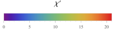
Figure 1: (Color online)The ratio $\chi^{\prime}$ of SNRs between postselected and non-postselected weak measurement vs coherent state’s parameters $\phi$ and r . Here we take $\varphi=\pi/4$ , $\theta=7\pi/9$ , and $s=10^{-5}$.

III.2 Squeezed vacuum state

Squeezed vacuum state is a typical quantum state. It has many applications in optical communication, optical measurement, and gravitational wave detection Milburn . Here, we assume that the initial pointer is squeezed vacuum state Scully which is defined by

$$|\xi\rangle=S(\xi)\left|0\right\rangle.$$ (20)

Here,

$$S(\xi)=\exp(\frac{1}{2}\xi^{\ast}a^{2}-\frac{1}{2}\xi a^{\dagger 2}),$$ (21)

where the squeezing parameter $\xi=\eta e^{i\delta}$ is an arbitrary complex number. After unitary evolution given in Eq. (5), the total system state is postselected to $|\psi_{f}\rangle$. Then, we obtain the following normalized final pointer state:

$$|\Psi_{f_{2}}\rangle=\frac{\gamma^{\prime}}{2}[(1+\langle A\rangle_{w})|\frac{s}{2},\xi\rangle+(1-\langle A\rangle_{w})|-\frac{s}{2},\xi\rangle],$$ (22)

where the normalization coefficient is given by

$$\gamma^{\prime}=\sqrt{2}[1+|\langle A\rangle_{w}|^{2}+(1-|\langle A\rangle_{w}|^{2})e^{-\frac{1}{2}s^{2}|\cosh\eta+e^{i\delta}\sinh\eta|^{2}}]^{-\frac{1}{2}}$$ (23)

and we note that $|\pm\frac{s}{2},\xi\rangle=D(\pm\frac{s}{2})S(\xi)|0\rangle$ is squeezed coherent state. Next we will calculate the expectation values of position and momentum operators under the normalized final pointer state $|\Psi_{f_{2}}\rangle$, and the results reads

$$\langle X\rangle_{f_{2}} \!\!= g|\gamma^{\prime}|^{2}\Re\langle A\rangle_{w}$$

$$-g|\gamma^{\prime}|^{2}\Im\langle A\rangle_{w}e^{-\frac{1}{2}s^{2}|\cosh\eta+e^{i\delta}\sinh\eta|^{2}}\sinh(2\eta)\sin\delta$$

and

$$\langle P\rangle_{f_{2}} = \frac{g|\gamma^{\prime}|^{2}}{2\sigma^{2}}\times$$

$$\Im\langle A\rangle_{w}e^{-\frac{1}{2}s^{2}|\cosh\eta+e^{i\delta}\sinh\eta|^{2}}(1+\sinh\left(2\eta\right)\cos\delta),$$

respectively. These formulas are valid not only in the weak measurement regime ($s\ll 1$), but also in strong measurement regime ($s\gg 1$).

Fig.2 shows the ratio $\mathcal{\chi}$ of SNR for squeezed pointer state between postselected and non- postselected weak measurements ($s\ll 1$) plotted as a function of $\delta$ and $\eta$ which are the parameters of squeezed state. One can see that when $\eta$ is large and near the points where $\delta=\frac{\pi}{2},\frac{3\pi}{2}$ the ratio $\mathcal{\chi}$ is much larger than unity. Evidently, this result indicates that squeezed pointer state is one of the quantum state candidates that can be utilized to improve the SNR in postselected rather than non-postselected weak measurement. This result was also confirmed in Ref. Pang(2014) .

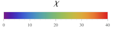
Figure 2: (Color online) The ratio $\mathcal{\chi}$ of SNRs between postselected and non-postselected weak measurements vs squeezed vacuum state’s parameters $\delta$ and $\eta$. Here we take $\varphi=\pi/4$, $\theta=7\pi/9$, and $s=10^{-5}$.

III.3 Schröinger cat state

Schröinger cat state is another typical quantum stateNeito which is a superposition of two coherent correlated states moving in opposite directions. Generally, there are two kinds of Schröinger cat statesDodonov ; even and odd Schröinger cat states. Even Schröinger cat state has very similar properties with squeezed state Hollen , since it has superpositions of photon number states with even numbers of quanta. Therefore, we consider the even Schröinger cat state as initial pointer sate to examine further the advantages of non-classical pointer state. The normalized even Schröinger cat state can be written as

$$|\Theta_{+}\rangle=K(|\alpha\rangle+|-\alpha\rangle),$$ (26)

where $|\pm\alpha\rangle$ are coherent states as defined in Eq. (10) which is characterized by $\alpha=re^{i\phi}$, and the normalization constant is

$$K=\frac{1}{\sqrt{2+2e^{-2|\alpha|^{2}}}}.$$ (27)

Following the same procedure as in previous sections, after taking unitary evolution given in Eq. (5), the outcome will then be projected to postselected state, $|\psi_{f}\rangle$. Then, we obtain the following normalized final pointer state

$$|\Psi_{f_{3}}\rangle=\frac{\kappa^{\prime}}{2}[(1+\langle A\rangle_{w})D(\frac{s}{2})+(1-\langle A\rangle_{w})D(-\frac{s}{2})]|\Theta_{+}\rangle,$$ (28)

where the normalization coefficient is given by

$$\kappa^{\prime} = [\frac{1}{2}(1+|\langle A\rangle_{w}|^{2})+K^{2}(1-|\langle A\rangle_{w}|^{2})\cos\left(2s\Im\left(\alpha\right)\right)e^{-\frac{s^{2}}{2}}$$ (29)

$$+\frac{K^{2}}{2}(1-|\langle A\rangle_{w}|^{2})(e^{-\frac{1}{2}|2\alpha+s|^{2}}+e^{-\frac{1}{2}|2\alpha-s|^{2}})]^{-\frac{1}{2}}.$$

By using Eq.(28) we calculate, in straightforward manner, the general forms of the expectation values for both conjugate position and momentum operators as

$$\langle X\rangle_{f_{3}} = 2\sigma|\kappa^{\prime}|^{2}K^{2}\times\{s\Re\langle A\rangle_{w}(1\!\!+e^{-2|\alpha|^{2}})\!$$

$$\!\!\!\!\!+2\Im\langle A\rangle_{w}\Re\left(\alpha\right)\sin(2s\Im\left(\alpha\right)e^{-\frac{1}{2}s^{2}}$$

$$-\Im\langle A\rangle_{w}\Im\left(\alpha\right)(e^{-\frac{1}{2}|2\alpha+s|^{2}}-e^{-\frac{1}{2}|2\alpha-s|^{2}}))\}$$

and

$$\langle P\rangle_{f_{3}} = \frac{|\kappa|^{2}K^{2}\Im\langle A\rangle_{w}}{2\sigma}\times\{\left(2\Re\left(\alpha\right)+s\right)e^{-\frac{1}{2}|2\alpha+s|^{2}}$$ (31)

$$\!\!\!\!+\!4\sin\left[2s\Im\left(\alpha\right)\right]\Im\left(\alpha\right)e^{-\frac{1}{2}s^{2}}\!\!\!\!+\!2s\cos\left[2s\Im\left(\alpha\right)\right]e^{-\frac{1}{2}s^{2}}$$

$$\!\!\!\!-\left(2\Re\left(\alpha\right)-s\right)e^{-\frac{1}{2}|2\alpha-s|^{2}}\},$$

respectively.

In Fig. 3, we plot the ratio $\chi$ of SNRs between postselected and non-postselected weak measurements for Schröinger cat pointer state. It is, clearly, indicating that when $r$ is increased and passed near $\phi=\frac{\pi}{4},\frac{3\pi}{4},\frac{5\pi}{4},\frac{7\pi}{4}$ , the ratio of SNRs is much larger than unity. Furthermore, when comparing Fig. 3 to Fig. 1, we find that the ratio $\chi$of non-classical Schröinger cat pointer state is higher than semi-classical coherent pointer state for the same parameters. This, evidently, leads to the improvement of SNR. However, when comparing between the two non-classical states in Fig. 2 and Fig. 3, one can see that these two Figures have some similarity, where both of them have the ratio $\chi$ larger than unity, while it get much stronger value for the case of squeezed state.

We have to emphasize at this point that we have also calculated the odd Schröinger cat pointer states but found that they have similar properties and results like the even Schröinger cat pointer states. And in order to avoid repetition, therfore, we just report the results of the even Schröinger cat states.

For the ratio of SNRs between postselected and non-postselected weak measurements, we can conclude that non-classical pointer states (squeezed vacuum, and Schröinger cat state) are better than semi-classical one (coherent sate) in order to improve the SNR in postselected weak measurements ($s\ll 1$) for complex weak values. This conclusion can be seen clearly from Fig. 1, Fig. 2 and Fig. 3.

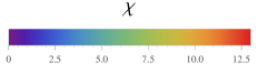
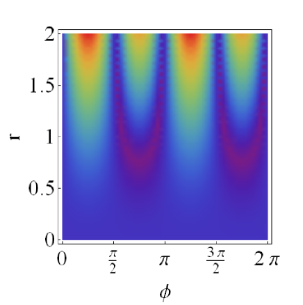
Figure 3: (Color online) The ratio $\mathcal{\chi}$ of SNRs between postselected and non post-selected measurement vs Schröinger cat state’s parameters $\phi$ and $r$. Here we take $\varphi=\pi/4$,$\theta=7\pi/9$, and $s=10^{-5}$.

The general expectation values of position and momentum operators for the above three pointer states - coherent, squeezed, and Schröinger cat states - can have the same property. This can be achieved if we assume the initial pointer state to be a zero-mean Gaussian beam (This corresponding to $r=0$ for coherent states and Schröinger cat state, and $\eta=0$ for squeezed vacuum state, respectively ), then all expressions reduced to

$$\langle X\rangle_{f}=\frac{g\Re\langle A\rangle_{w}}{\mathcal{Z}},$$ (32)

and

$$\langle P\rangle_{f}=\frac{g\Im\langle A\rangle_{w}}{2\sigma^{2}\mathcal{Z}}e^{-\frac{1}{2}s^{2}}.$$ (33)

Here,

$$\mathcal{Z=}1+\frac{1}{2}(1-|\langle A\rangle_{w}|^{2})(e^{-\frac{1}{2}s^{2}}-1).$$ (34)

This result is given in Nakamura’s work Nakamura(2012) .

A remaining issue is to examine the connection between weak and strong postselected measurement. Thus, we plot the $SNR_{X}^{p}$, which is defined in Eq.(8), as function of arbitrary measurement strength parameter $s$ and preselection angle $\theta$. From Fig. 4, particularly for squeezed vacuum pointer state, we can see that at $\theta=\pi/2$ the $SNR_{X}^{p}$ increase with the increase of $s$, this is the strong measurement result. The reason is that at $\theta=\pi/2$ the preselected state Eq.(16) is the eigenstate of operator $\sigma_{x}$ which have eigenvalue $+1$. This figure doesn’t only make the connection between weak and strong postselected measurement, but also indicates that non-classical pointer states are also good enough comparing with semi-classical ones in generalized von Neumann measurementTurek .

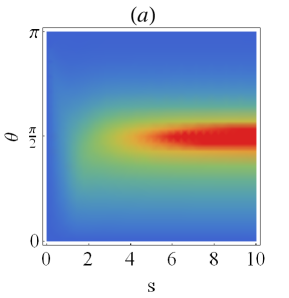
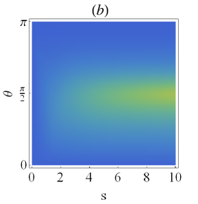
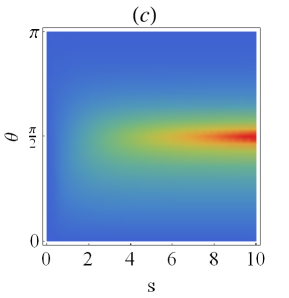
Figure 4: (Color online) The $R_{X}^{p}$ for arbitrary measurement strength parameter $s$, and $\theta$ for different weak values. Here, we take $\varphi=0$ and $N=1$. (a) For coherent pointer state, $r=1$, $\phi=\pi/4$. (b) For Schröinger cat pointer sates, $r=1,$ $\phi=\pi/4$. (c) For squeezed vacuum pointer state, $\eta=1,$$\delta=\pi/4$.

IV Quantum Fisher information

Fisher information is the maximum amount of information about the parameter that we can extract from the system. For a pure quantum state $|\psi_{s}\rangle$, the quantum Fisher information estimating $s$ is

$$F^{(Q)}=4[\langle\partial_{s}\psi_{s}|\partial_{s}\psi_{s}\rangle-|\langle\psi_{s}|\partial_{s}\psi_{s}\rangle|^{2}].$$ (35)

where the state $|\psi_{s}\rangle$ represents the final pointer states of the system. Here, this can be used for coherent, squeezed vacuum, or Schröinger cat states when only dealing with the postselected weak measurement in the first order evolution of unitary operator $e^{-ig\hat{A}\otimes\hat{P}}$. Here, $s\equiv g/\sigma$ is the measurement strength parameter which directly related to coupling constant $g$ in our Hamiltonian of Eq.(1).

The variance of unknown parameter $\Delta s$ is bounded by the Cramer-Rao bound

$$\Delta s\geq\frac{1}{NF^{(Q)}},$$ (36)

where $N$ is the total number of measurements. Thus, the Fisher information set the minimal possible estimate for parameter $s$, while higher Fisher information means better estimation. In weak measurement, if we consider the successful postselection probability, then Fisher information would be $F_{p}^{(Q)}=P_{s}F^{(Q)}$. In Ref.Pang(2014) , one can find general proof showing that quantum Fisher information is higher in postselected rather than non-postselected weak measurement. Thus, we just focus on the postselected weak measurement process and look into Fisher information for semi-classical and non-classical pointer states.

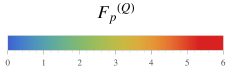
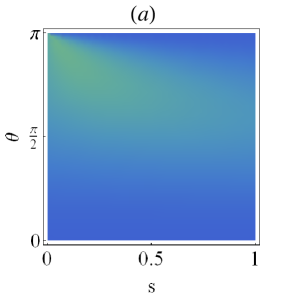
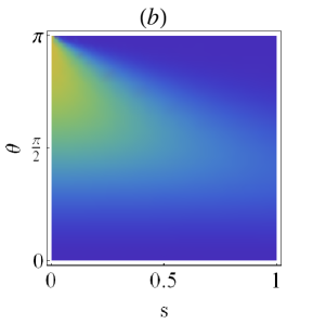
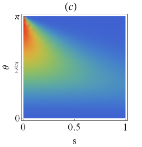
Figure 5: (Color online) The quantum Fisher information in weak measurement regime vs measurement strength parameter $s$ and $\theta$ for different weak values. Here, we take $\varphi=\pi/4$ and $N=1$. (a) For coherent pointer state, $r=1$, $\phi=\pi/4$. (b) Schröinger cat pointer sates, $r=1,$ $\phi=\pi/4$. (c) For squeezed vacuum pointer state, $\eta=1,$$\delta=\pi/4$.

We proceed investigating the variation of Fisher information in weak measurement regime for different weak values. Our numerical results in Fig. 5 show that the quantum Fisher information is higher in weak measurement regime ($s\ll 1$) when the preselection and postselection state almost orthogonal. The other important result is that the non-classical pointer states have more advantages over the semi-classical ones which in turn leads to better estimation process.

V Conclusion

In summary, we give a general expressions for the shifted values of position and momentum operators for different pointer states (coherent, squeezed vacuum, and Schröinger cat states), these expressions are valid in weak and strong measurement regimes. In the next step, we investigate the SNR and the quantum Fisher information only in weak measurement regime. We find that if we take initial state as zero mean Gaussian state, our general expressions of shifted values would be reduced to Eq. (32) and Eq. (33), which are given in Ref. Nakamura(2012) . By giving the ratio of SNR between postselected and non- postselected weak measurement, we find that postselected weak meaurement process for non-classical pointer states give more infromation about the system comparing to the non-postselected process. This result keeps consistent with S. Pang et al’s work Pang(2014) . If one wants to quantify the quantum Fisher information in order to improve the precision of unknown parameter estimation, then he can consider using non-classical pointer sate and avoiding the semi-classical one.

- (1) Y. Aharonov, D.Z. Albert, and L. Vaidman, Phys. Rev. Lett. 60, 1351 (1988).
- (2) Y. Aharonov, D. Rohrlich, Quantum Paradoxes- Quantum Theory for the Perplexed (Wiley-VCH, Weinheim, 2005).
- (3) J. Tollaksen et al., New J. Phys. 12, 013023 (2010).
- (4) N.W. M. Ritchie, J. G. Story, and R.G. Hulet, Phys. Rev. Lett. 66, 1107 (1991).
- (5) O. Hosten and P. Kwiat, Science 319, 787 (2008).
- (6) P. B. Dixon, D. J. Starling, A. N. Jordan, and J. C. Howell, Phys. Rev. Lett. 102, 173601 (2009).
- (7) D. J. Starling, P. B. Dixon, A. N. Jordan, and J. C. Howell, Phys. Rev. A 80, 041803(R) (2009).
- (8) J. M. Hogan, J. Hammer, S.-W. Chiow, S. Dickerson, D. M. S. Johnson, T. Kovachy, A. Sugarbaker, and M. A. Kasevich, Opt. Lett. 36, 1698 (2011).
- (9) M. Pfeifer, and P.Fischer, Opt.Exp 19, 16508 (2011).
- (10) L. Zhou, Y. Turek, C. P. Sun, and F. Nori, Phys. Rev. A 88, 053815 (2013).
- (11) D. J. Starling, P. B. Dixon, A. N. Jordan, and J. C. Howell, Phys. Rev. A 82, 063822 (2010).
- (12) D. J. Starling, P. B. Dixon, N. S. Williams, A. N. Jordan, and J. C. Howell, Phys. Rev. A 82, 011802(R) (2010).
- (13) O. S. Magaña-Loaiza, M. Mirhosseini, B. Rodenburg, and R. W. Boyd, Phys. Rev. Lett. 112, 200401 (2014).
- (14) B. de Lima Bernardo, S. Azevedo, and A. Rosas. Phys. Lett. A 378, 2029 (2014).
- (15) G. I. Viza, J. Martinez-Rincon, G. A. Howland, H. Frosting, I. Shomroni, B. Dayan, and J. C. Howell, Opt. Lett. 38, 2949 (2013).
- (16) P. Egan and J. A. Stone, Opt. Lett. 37, 4991 (2012).
- (17) Y. Aharonov, A. Botero, S. Popescu, B. Reznik, and J. Tollaksen, Phys. Lett. A 301, 130 (2002).
- (18) J. S. Lundeen and A. M. Steinberg, Phys. Rev. Lett. 102, 020404 (2009).
- (19) K. Yokota, T. Yamamoto, M. Koashi, and N. Imoto, New J. Phys. 11, 033011 (2009).
- (20) K. J. Resch, J. S. Lundeen, and A. M. Steinberg, Phys. Lett. A 324, 125 (2004).
- (21) Y. Aharonov and D. Rohrlich, Quantum Paradoxes: Quantum Theory for the Perplexed (Wiley-VCH, Weinheim, 2005).
- (22) Y. Aharonov and L. Vaidman, in Time in Quantum Mechanics, Vol. 1, edited by J. G. Muga, R. Sala Mayato, and I. L. Egusquiza (Springer, Berlin Heidelberg, 2008), p. 399.
- (23) Y. Aharonov and J. Tollaksen, in Vision of Discovery: New Light on Physics, Cosmology, and Consciousness, edited by R. Y. Chiao, M. L. Cohen, A. J. Legget, W. D. Phillips, and C. L. Harper, Jr. (Cambridge University Press, Cambridge, 2011), p. 105.
- (24) A. Hosoya and Y. Shikano, J. Phys. A 43, 385307 (2010).
- (25) Y. Shikano and S. Tanaka, Europhys. Lett. 96, 40002 (2011).
- (26) H. F. Hofmann and C. Ren, Phys. Rev. A 87, 062109 (2013).
- (27) J. S. Lundeen, B. Sutherland, A. Patel, C. Stewart, and C. Bamber, Nature 474, 188 (2011).
- (28) J. S. Lundeen, and C. Bamber, Phys. Rev. Lett. 108, 070402 (2012).
- (29) S. Kocsis, B. Braverman, S. Ravets, M. J. Stevens, R. P. Mirin, L. K. Shalm, and A. M. Steinberg, Science 332, 1170 (2011).
- (30) B. Braverman and C. Simon, Phys. Rev. Lett. 110, 060406 (2013).
- (31) J. Z. Salvail, M. Agnew, A. S. Johnson, E. Bolduc, J. Leach, and R. W. Boyd, Nat. Photon. 7, 316 (2013).
- (32) M. Malik, M. Mirhosseini, M. P. J. Lavery, J. Leach, M. J. Padgett, and R. W. Boyd, Nat. Commun. 5, 3115 (2014).
- (33) A. Palacios-Laloy, F. Mallet, F. Nguyen, P. Bertet, D. Vion, D. Esteve, and A. N. Korotkov, Nat. Phys. 6, 442 (2010).
- (34) Y. Suzuki, M. Iinuma, and H. F. Hofmann, New J. Phys. 14, 103022 (2012).
- (35) J. Dressel, C. J. Broadbent, J. C. Howell, and A. N. Jordan, Phys. Rev. Lett. 106, 040402 (2011).
- (36) M. E. Goggin, M. P. Almeida, M. Barbieri, B. P. Lanyon, J. L. O’Brien, A. G. White, and G. J. Pryde, Proc. Natl. Acad. Sci. U. S. A. 108, 1256 (2011).
- (37) C. Emary, N. Lambert, and F. Nori, Rep. Prog. Phys. 77, 016001 (2014).
- (38) J. P. Groen, D. Riste, L. Tornberg, J. Cramer, P. C. de Groot, T. Picot, G. Johansson, and L. DiCarlo, Phys. Rev. Lett. 111, 090506 (2013).
- (39) L. A. Rozema, A. Darabi, D. H. Mahler, A. Hayat, Y. Soudagar, and A. M. Steinberg, Phys. Rev. Lett. 109, 100404 (2012).
- (40) F. Kaneda, S.-Y. Baek, M. Ozawa, and K. Edamatsu, Phys. Rev. Lett. 112, 020402 (2014).
- (41) Y. Shikano, in Measurement in Quantum Mechanics, edited by M. R. Pahlavani (InTech, Rijeka, Croatia, 2012), p. 75, arXiv:1110.5055.
- (42) A. G. Kofman, S. Ashhab, and F. Nori, Phys. Rep. 520, 43 (2012).
- (43) J. Dressel, M. Malik, F. M. Miatto, A. N. Jordan, and R. W. Boyd, Rev. Mod. Phys. 86, 307 (2014).
- (44) G. C. Knee and E. M. Gauger, Phys. Rev. X 4, 011032 (2014).
- (45) X. Zhu, Y. Zhang, S. Pang, C. Qiao, Q. Liu, and S. Wu, Phys. Rev. A 84, 052111 (2011).
- (46) S. Pang and T. A. Brun, arXiv:1409.2567 (2014).
- (47) K. Nakamura, A. Nishizawa, and M. K. Fujimoto, Phys. Rev. A 85, 012113 (2012).
- (48) Y. Turek, H. Kobayashi, T. Akutsu, C. P. Sun, and Y. Shikano, New J. Phys 17, 083029 (2015).
- (49) D.F. Walls and G. J. Milburn, Quantum Optics (Springer, Berlin, 1994); K. Goda, O. Miyakawa, E. E. Mikhailov, S. Saraf, R. Adhikari, K. McKenzie, R. Ward, S. Vass, A. J. Weinstein, and N. Mavalvala, Nat. Phys. 4, 472 (2008); R. Loudon and P.L.Knight, J. Mod. Opt. 34, 709 (1987).
- (50) Scully, M. O., and M. S. Zubairy, Quantum Optics (Cambridge University Press, Cambridge, 197).
- (51) M. M. Nieto and D. R. Truax, Phys. Rev. Lett. 71, 2843 (1993).
- (52) V. V. Dodonov, I. A. Malkin, and V. I~ Man’ko, Physica 72, 597 (1974); I. A. Malkin and V. I. Man’ko, Dynamical Symmetries and Coherent States of Quantum Systems (Nauka, Moscow, 1979).
- (53) J. N. Hollenhorst, Phys. Rev. D 19, 1669 (1979).