Intracellular impedance measurements reveal non-ohmic properties of the extracellular medium around neurons

Running title: Impedance measurements in cerebral cortex

Corresponding author: Alain Destexhe, UNIC, CNRS, 1 Avenue de la Terrasse,
91190 Gif sur Yvette, France.  Tel: +33 1 69 82 34 35  destexhe@unic.cnrs-gif.fr

Keywords: Cerebral cortex, impedance, electrophysiology, computational models,
local field potential, extracellular

Conflict of interest: None

Abstract

The electrical properties of extracellular space around neurons are important to understand the genesis of extracellular potentials, as well as for localizing neuronal activity from extracellular recordings. However, the exact nature of these extracellular properties is still uncertain. We introduce a method to measure the impedance of the tissue, and which preserves the intact cell-medium interface, using whole-cell patch-clamp recordings in vivo and in vitro. We find that neural tissue has marked non-ohmic and frequency-filtering properties, which are not consistent with a resistive (ohmic) medium, as often assumed. The amplitude and phase profiles of the measured impedance are consistent with the contribution of ionic diffusion. We also show that the impact of such frequency-filtering properties is possibly important on the genesis of local field potentials, as well as on the cable properties of neurons. The present results show non-ohmic properties of the extracellular medium around neurons, and suggest that source estimation methods, as well as the cable properties of neurons, which all assume ohmic extracellular medium, may need to be re-evaluated.

Introduction

The genesis and propagation of electric signals in brain tissue depend on its electric properties, which can be simply resistive (ohmic) or more complex, such as capacitive, polarizable or diffusive. The exact nature of these electric properties is important, because non-resistive media will necessarily impose frequency-filtering properties to electric signals [1, 2], and therefore will influence any source localization. These electric properties were measured using metal electrodes, which provided measurements suggesting that the brain tissue is essentially resistive [3, 4, 5]. However, the electrical behavior of tissue and electrodes can be easily confused [6]; efforts in the direction of distinguishing or separating them abound ([7, 8, 9]). Another experimental approach using very low-impedance probes revealed marked frequency dependence of conductivity and permittivity [10, 11]. Indirect evidence for non-resistive media were also obtained [12, 13, 14], and also indicated a marked frequency dependence.

To explain these discrepancies, we hypothesize that the apparently contradictory results are due to the fact that different measurement methods were used. The use of metal electrodes represents a non-physiological interface for interacting with the surrounding tissue, while in reality, neurons interact with the extracellular medium by exchanging ions through membrane ion channels and pumps. To respect as much as possible these natural conditions, we have measured the tissue impedance using a neuron as a current source, thereby respecting the natural interface. This intracellular measurement provides a measurement of a global cell impedance, which contains the membrane impedance and the impedance of the extracellular medium. This global intracellularly-measured impedance can also be defined as the impedance as seen by the cell.

Figure 1 illustrates this concept and the recording setup needed to record this global impedance intracellularly, in vitro (Fig. 1A) or in vivo (Fig. 1B). Fig. 1C gives two circuit configurations for this system, emphasizing three impedances: $Z_{i}$ is the impedance of the intracellular medium (cytoplasm), $Z_{e}$ is the extracellular impedance, and $Z_{RC}$ is the membrane impedance, represented by a simple resistance-capacitance (RC) circuit (left), or a more complex circuit including dendritic compartments all described by different RC circuits (right). An intracellular electrode will measure a global combination of these impedances, In the following of the text, we will call this global impedance the “global intracellular impedance”.

A central point of our study is that this global intracellular impedance is different than the electrical impedances measured by metal electrodes, which we refer here as “metal-electrode impedance”. We will investigate whether the intracellularly-measured impedance reveals more complex electrical properties than with metal electrodes, which could possibly explain the discrepancies described above. The global intracellular impedance provides not only a realistic estimate of the electrical properties the extracellular medium, but it is also closer to the natural conditions, and could be a useful physical parameter to determine a more precise source localization of cerebral electric signals, and to model the propagation of electrical signals in the extracellular space or in dendritic trees, as we illustrate here.

Materials and Methods

Animals

Maintenance, surgery and all experiments were performed in accordance with the local animal welfare committees (Center for Interdisciplinary Research in Biology and EU guidelines, directive 2010/63/EU, and regional ethics committee "Ile-de-France Sud” (Certificate 05-003)). Every precaution was taken to minimize stress and the number of animals used in each series of experiments. Animals were housed in standard 12 hours light/dark cycles and food and water were available ad libitum.

In vitro electrophysiology

Brain slice preparation.
Visual cortex. 300 $\mu$m-thick coronal brain slices of juvenile mice ($P_{12-16}$ Swiss mice bred in the CNRS Animal Care facility, Gif-sur-Yvette ; French Agriculture Ministry Authorization: B91-272-105) were obtained with a Leica VT 1200S microtome (Leica Biosystems, Wetzlar, Germany). Slices were prepared at 4${\,}^{\circ}C{\,}$in the following medium (in mM): choline chloride 110, KCl 2.55, NaH₂PO₄ 1.65, NaHCO₃ 25, dextrose 20, CaCl₂ 0.5, MgCl₂ 7. Slicing started 2 mm from the posterior limit of olfactory bulb, and ended 3.9mm further. Before recordings, slices were incubated at 34${\,}^{\circ}C{\,}$in artificial cerebro-spinal fluid (ACSF) of the following composition (in mM): NaCl 126, KCl 3, NaHC$O_{3}$ 26, NaH₂P$O_{4}$ 1.25, myo-inositol 3, sodium pyruvate 2, L-ascorbate de sodium 0.4 ; dextrose, 10. The slicing and recording solution was bubbled with 95% O₂ and 5% CO₂, for a final pH of 7.4.

Dorsal striatum. Horizontal brain slices with a thickness of 330 $\mu$m were prepared from rats ($P_{23-30}$ OFA rats (Charles River, L’Arbresle, France), using a vibrating blade microtome (VT1200S, Leica Microsystems, Nussloch, Germany). Brains were sliced in a 95% O₂ / 5% CO₂-bubbled, ice-cold cutting solution containing (in mM): NaCl 125, KCl 2.5, glucose 25, NaHCO₃ 25, NaH₂PO₄ 1.25, CaCl₂, MgCl₂ 1, pyruvic acid 1, and then transferred into the same solution at 34${\,}^{\circ}C{\,}$.

Electrophysiological recordings.
Patch-clamp recordings in pyramidal cells of visual cortex from mice were performed as followed. Slices were superfused at 2 mL/min with the same ACSF solution that was used for incubation. Bath temperature of the submerged chamber was maintained at 34 ${\,}^{\circ}C{\,}$using a TC-344B temperature controller (Warner Instruments Company, Hamden, CT, USA). Neurons in slices of the mouse visual cortex ($P_{12-16}$) were identified with an upright microscope (Axioscope FS, Zeiss, Germany), an infrared camera (C750011, Hamamatsu Photonics, Japan) and an infrared filter. Patch-clamp in the whole-cell current clamp configuration in layer V pyramidal neurons was performed simultaneously with an extracellular recording using a 3 M$\Omega$ patch pipette (Fig. 1A). The latter was located within a close vicinity ($\approx 30~{}\mu m$) of the patched cell. All results were indifferent to the distance between the reference electrode and the patched cells, as potential variations on the extracellular electrode did not excede 1% of the variations of the intracellular potential. Borosilicate pipettes (1B150F4, World Precision Instruments, Inc., Sarasota, Florida, U.S.) of 5-8 M$\Omega$ impedance were used for whole-cell recordings and contained the intracellular solution (in mM): Hepes 10, EGTA 1, K-gluconate 135, MgCl₂ 5, CaCl₂ 0.1, with osmolarity of 308 mOsm and a pH of 7.3. Serial resistance was not compensated for. Recordings were performed with a Multiclamp 700B amplifier (Axon Instruments Inc., California, U.S.), filtered at 10 kHz with a built-in Bessel filter, and sampled at 25 kHz. Data acquisition and stimulation were performed with a National Instruments BNC 2090 A card, and the software ELPHY (G. Sadoc, CNRS, UNIC, France).

Patch-clamp recordings in medium-sized spiny neurons of dorsal striatum from rats were performed as previously described [15]. Briefly, borosilicate glass pipettes of 6-8M impedance contained for whole-cell recordings (in mM): K-gluconate 105, KCl 30, HEPES 10, phosphocreatine 10, ATP-Mg 4, GTP-Na 0.3, EGTA 0.3 (adjusted to pH 7.35 with KOH). The composition of the extracellular solution was (mM): NaCl 125, KCl 2.5, glucose 25, NaHCO₃ 25, NaH₃PO4 1.25, CaCl₂ 2, MgCl₂ 1, pyruvic acid 10, bubbled with 95% O₂ and 5% CO₂. Signals were amplified using EPC10-3 amplifiers (HEKA Elektronik, Lambrecht, Germany). All recordings were performed at 34${\,}^{\circ}C{\,}$using a temperature control system (Bath-controller V, Luigs & Neumann, Ratingen, Germany) and slices were continuously superfused at 2 ml/min with the extracellular solution. Slices were visualized on an Olympus BX51WI microscope (Olympus, Rungis, France) using a 4x/0.13 objective for the placement of the stimulating electrode and a 40x/0.80 water-immersion objective for localizing cells for whole-cell recordings. During the experiment, individual striatal and cortical neurons were identified using infrared-differential interference contrast microscopy with a CCD camera (Optronis VX45; Kehl, Germany). Serial resistance was not compensated for. Current-clamp recordings were filtered at 2.9 kHz and sampled at 16.7 kHz using the Patchmaster v2x73 program (HEKA Elektronik). Stimuli in current-clamp mode underwent a high cut 10kHz filter before being applied. Recordings were made with EPC 10-3 amplifiers (HEKA Elektronik; Lambrecht, Germany) with a very high input impedance ($1~{}T\Omega$) to ensure there was no appreciable signal distortion imposed by the high impedance electrode (Nelson et al., 2008). Sinusoidal stimuli were then introduced in whole-cell patch-clamp to the patched cell.

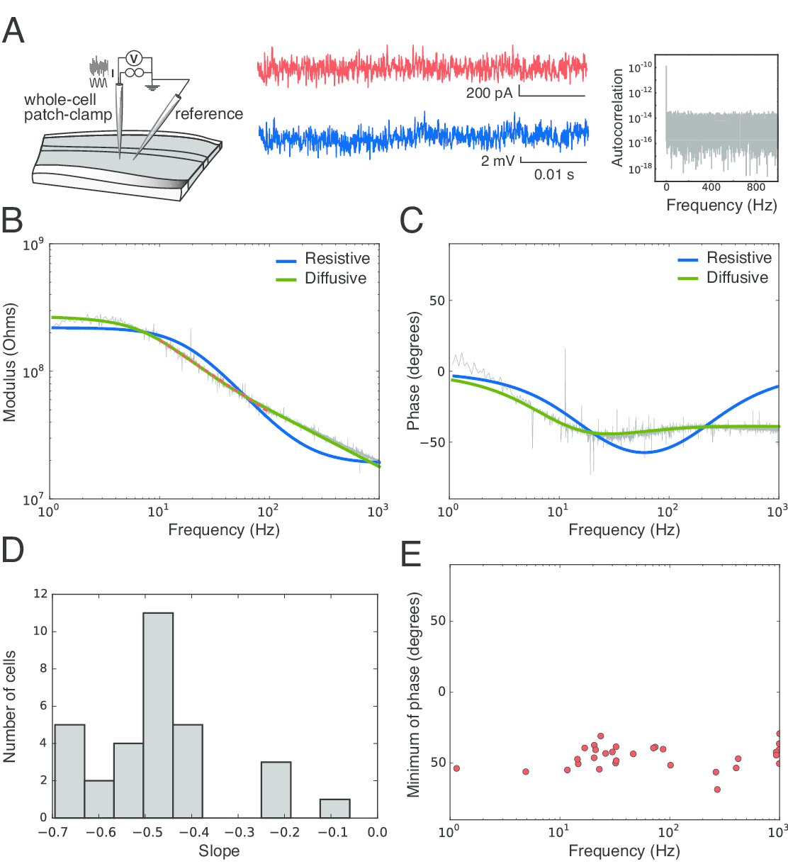
Figure 2: Global intracellular impedance of cortical neurons recorded in vitro (current clamp). A: Left: Scheme of the experimental setup; Middle: example signals; A gaussian white noise current signal (red, amplitude: $\pm$100 pA) was injected repeatedly in patched neurons while recording the intracellular potential (blue). For each 20 seconds period, we computed the impedance as the ratio of measured voltage on injected current ($Z_{mes}=\frac{V_{intra}}{i_{inj}}$) and averaged on 30 periods. Acquisition was performed at 20 kHz. Right: Autocorrelation of the injected white noise current in Fourier space. B: modulus of $Z_{eq}$ (log scale) represented as a function of frequency ($log_{10}(f)$), for white noise current injection. C: Fourier phase of $Z_{eq}$, in the same experiment. The different curves shows the best fit of two models to the experimental data (blue: resistive, green: diffusive). Parameters of the models: i) Resistive: ${\color[rgb]{0,0,0.65}R_{m}}=~{}200M\Omega$, ${\color[rgb]{0,0,0.65}C_{m}}=45~{}pF$, ${\color[rgb]{0,0,0.65}R_{e}}=19~{}M\Omega$; ii) Diffusive: ${\color[rgb]{0,0,0.65}R_{m}}=180~{}M\Omega$, ${\color[rgb]{0,0,0.65}C_{m}}=~{}110pF$, ${\color[rgb]{0,0,0.65}A}=~{}99M\Omega$, ${\color[rgb]{0,0,0.65}B}=3.8~{}M\Omega$, ${\color[rgb]{0,0,0.65}f_{W}}=36~{}Hz$. ${\color[rgb]{0,0,0.65}A}$, ${\color[rgb]{0,0,0.65}B}$ and ${\color[rgb]{0,0,0.65}f_{W}}$ are parameters of the diffusive impedance scaling respectively its amplitude, phase, and cutoff frequency. D: Distribution of the slopes of $Z_{eq}$ fitted between 20 and 200 Hz (linear fit, red dashed lines on the figures). E: Coordinates of the minima of the Fourier phases for each cell.

This configuration enables estimating the extracellular impedance, according to the circuit displayed in Fig. 1C. To this end, a white noise current stimulus was injected into the recorded cell and the impedance was calculated based on this current injection (see Fig. 2A). 20 to 120 seconds of Gaussian white noise with zero mean and 100 pA variance was injected (results were similar for 30 and 200 pA variance). For each cell, we injected 15 to 30 times the same sequence of white noise (“frozen noise”) and averaged the measured voltages. This enhanced the signal to noise ratio without altering the results. Figure 2A (right panel) shows the very low autocorrelation of the injected currents, being thus a good approximation of white noise. To verify that the same results can be obtained using a different protocol, we also performed slice experiments using sinusoid current stimuli, at different frequencies. This set of experiments was performed following the methods previously published [14, 16]. Namely, sine waves of 12 different frequencies were tested, varying approximately evenly on a logarithmic scale ranging from 6 Hz to 926 Hz. Up to 500 traces of 100 to 1500 ms in length were averaged before recording the data to disk for offline analyses. Longer stimulus lengths and more traces were necessary for the low frequency stimuli. The order of the presentation of the frequencies was randomized. Stimuli were introduced with the patch electrode in current-clamp mode. The injected current amplitudes ranged from 200 to 300 pA. Before conducting experiments, we verified via control recordings with an external signal generator in the bath without a slice that any amplitude changes or phase shifts in the recordings across frequencies induced by the amplifier and recording hardware were negligible [16].

In vivo electrophysiology

Surgical preparation of animals.
Adult rats (P40-90) were placed in a stereotaxic apparatus (Unimecanique, Asnières, France) after anesthesia induction with a 400mg/kg intra-peritoneal injection of chloral hydrate (Sigma-Aldrich, Saint-Quentin Fallavier, France). A deep anesthesia maintenance was ensured by intra-peritoneal infusion on demand of chloral hydrate delivered with a peristaltic pump set at 60mg/kg/hour turned on one hour after induction. Proper depth of anesthesia was assessed regularly by testing the cardiac rhythm, EcoG activity, the lack of response of mild hindpaw pinch and the lack of vibrissae movement. The electrocardiogram was monitored throughout the experiment and body temperature was maintained at 36.5${\,}^{\circ}C{\,}$by a homeothermic blanket.

Two craniotomies were performed, one for the insertion of a reference electrode in the somatosensory cerebral cortex (layer2/3) and one to allow the whole-cell recordings in the contralateral cortex (layer 5). For whole-cell recordings, a 2x2 mm craniotomy was made to expose the left posteromedial barrel subfield at the following coordinates: posterior 3.0-3.5 mm from the bregma, lateral 4.0-4.5 mm from the midline. The dura was opened and the craniotomy was filled with low melting point paraffine after each time lowering a recording pipette. To increase recording stability the cisterna magna was drained.

Electrophysiological recordings

Borosilicate glass pipettes of $5-8M\Omega$ impedance for blind whole-cell recordings contained (in mM): K-gluconate 105, KCl 30, HEPES 10, phosphocreatine 10, ATP-Mg 4, GTP-Na 0.3, EGTA 0.3 (adjusted to pH 7.35 with KOH). Signals were amplified using an EPC10-plus-2 amplifier (HEKA Elektronik). Series resistance was not compensated for. Current-clamp recordings were filtered at 2.5 kHz and sampled at 5 kHz using the Patchmaster v2x32 program (HEKA Elektronik). Whole-cell recordings were performed in pyramidal cells of the somatosensory cortex in layer IV/V (depth from the dura: 0.8-1.2 mm) (Fig. 1B). Recorded cells were identified as pyramidal cells according to their characteristic spiking pattern. The reference was a silver wire placed in the contralateral hemisphere. Note that for both in vivo and in vitro experiments, the reference electrode is passive, just measuring the extracellular voltage, and thus the exact nature of this reference is not critical. Accordingly, the same configuration using a silver microwire gave similar results in vitro (not shown).

It is important, however, that the reference electrode be placed in the brain tissue, so that the estimated extracellular impedance is not influenced by other tissues. Thus, as in the in vitro experiments, this intracellular-extracellular configuration enables estimating the extracellular impedance. An important difference with in vitro, is that in vivo the current can flow more freely in 3 dimensions, and is closer to natural conditions. Another difference is that in vivo, the system is not silent but displays prominent spontaneous activity. To limit this contribution, we have used a “frozen noise” protocol, where identical sequences of white noise stimuli were injected repetitively, and the sequences averaged.

The main purpose of this experiment was to estimate $Z_{eq}$, the equivalent impedance between the Ag-AgCl electrode and the ground. In the case of a simple, single-compartment neuron, it can be formally defined as $Z_{eq}=Z_{i}+Z_{RC}+Z_{e}$. This was achieved by applying two protocols of subthreshold current injection:

1. The “frozen noise” protocol consisting in the same template of 20 seconds of a white noise current (repeated 50 times with 2 s intervals between stimulations and averaged). Sequences in which spikes were induced were discarded.

2. Sinusoidal current at fixed frequencies ranged from 6 Hz to 926 Hz (similar to those used in in vitro experiments). The order of the presentation of the frequencies was randomized.

For the frozen noise and sinusoidal stimuli, the injected currents were tuned for each neurons to evoke voltage response of magnitude ranged between 2 and 6 mV. Note that in some experiments we injected a hyperpolarizing current (of maximum amplitude $-150$ pA) to prevent suprathreshold activity during application of stimuli.

Analysis

All analyses were performed using Python (Python Software Foundation, Wolfeboro Falls, New Hampshire, USA), the Scipy Stack and Spyder (Pierre Raybaut, The Spyder Development Team).

In vitro and in vivo patch-clamp - sine waves experiments

For each frequency and current intensity, the recorded voltages and injected intensities were averaged and fit with sines using the optimize package included in Scipy. The adequation between data and the fitted sine waves was checked by human intervention for every set of data. The voltage and current were represented respectively as $V(t,f)=V_{0}sin(2\pi ft+\phi_{v})$ and $I(t,f)=I_{0}sin(2\pi ft+\phi_{i})$). The impedance for a given frequency was thus given by $Z(f)=\frac{V_{0}}{I_{0}}e^{i(\phi_{v}-\phi_{i}})$.

In vitro and in vivo patch-clamp - white noise experiments

Several models were fit to the experiments. First, we used a purely resistive model (Fig. 1, bottom left) in which the intracellular impedance $Z_{i}$ can be considered zero and the extracellular impedance $Z_{e}$ was a small resistance ($R_{e}$). The equivalent impedance is thus given by:

$${\color[rgb]{0,0,0.65}Z_{eq,1}(\omega)=\frac{R_{m}}{1+i\omega\tau_{m}}+R_{e}}$$ (1)

Second, we combined $Z_{i}$ and $Z_{e}$ as a diffusive term. Rather than trying to find an elusive general solution for the usual Nernst-Planck equation [17], we used a first-order approximation for ionic diffusion. The impedance of an electrolyte showing non-negligible ionic diffusion was derived by Warburg [18, 19], and yielded a modulus scaling in $1/\sqrt{\omega}$ and a constant phase. Similar derivations have been performed in different symmetries [20, 21, 22]. Note that the latter derivations model the impedance of ionic accumulations close to the membrane, by using a first-order approximation of the electric potential generated by ionic species following Boltzmann distributions.

This “diffusion” impedance has been observed experimentally (reviewed in ref. [7]), and can be modeled in spherical symmetry by two components scaling the modulus and phase ($A$ and $B$), and a cutoff frequency $f_{W}=\omega_{W}/2\pi$:

$${\color[rgb]{0,0,0.65}Z_{W}(\omega)=\frac{A+iB}{1+\sqrt{\omega/\omega_{W}}}}$$ (2)

This leads to the following expression for the equivalent impedance:

$${\color[rgb]{0,0,0.65}Z_{eq,2}(\omega)=\frac{R_{m}}{1+i\omega\tau_{m}}+\frac{A+iB}{1+\sqrt{i\frac{\omega}{\omega_{W}}}}}$$ (3)

To take into account the fact that some of the current can flow through the dendrites of the cell, we define a dendritic input impedance $Z_{d}$ (see Fig. 1D, right), namely the impedance of the dendritic tree seen by currents leaving the soma. These currents will flow downwards the gradient potential from the intracellular potential ($V_{intra}$) to the reference ($V_{ref}=0$). Thus, $Z_{d}$ is defined by $V_{intra}/i_{d}^{g}$, where $i_{d}^{g}$ is the generalized axial current in the dendrite at the level of the soma, and $V_{intra}$ is the intracellular potential at the soma. Note that we consider here $V_{intra}$ as not necessarily equal to the transmembrane potential ($V_{m}$) because we take $V_{e}$, the potential of the extracellular medium, into account. We then consider separately the resistance and capacitance of the soma ($R_{s}$,$C_{s}$) and the impedance of the dendrite. The equivalent impedance is then: $Z_{eq,3-4}(\omega)=\frac{Z_{d}Z_{s}}{Z_{d}+Z_{s}}+Z_{i}+Z_{e}$, where $Z_{s}(\omega)=\frac{R_{s}}{1+i\omega\tau_{m}}$ is the impedance of the soma, $Z_{eq,3}$ and $Z_{eq,4}$ are the impedances for resistive and diffusive media respectively. A description of these different models can be found in the next section; parameters for each of these models are listed in Table 1.

Fitting models with and without dendrites

Two types of models were fit to the experimental measurements, as illustrated in Fig. 1C: a single-compartment model, and a model including a dendritic segment. Dendritic filtering has been proposed to explain the frequency-dependence of LFPs [23, 24]; thus, current flowing in the dendrites could be involved in shaping the measured impedance, which would in turn influence the frequency-dependence of local field potentials. We tested this possible influence by considering models that include an equivalent dendritic compartment, which has been shown to be electrically equivalent to a full dendritic tree [25, 26], leading to a “ball-and-stick” type model (see right circuit in Fig. 1C).

In order to fit the models to experimental data, several traditional fitting methods were tested (e.g. Newton-Gauss, Levenberg-Marquardt, conjugate gradient, simplex…) but were plagued with three main problems: a long computation time (with 4 parameters or more), a tendency to get trapped in local minima, and an extreme sensitivity to the first estimation of model parameters. We thus developed a probabilistic, non-iterative method that had none of these problems.

We proceeded as follows: 1. For each parameter, we defined a domain of acceptable values, keeping it very large (too much restriction on a parameter is a symptom of analytical bias). 2. We drew random sets of parameters (between 500 and 5000), e.g $P_{j}=(R_{m},C_{m},A,B,f_{W}...)$, and computed the theoretical impedance spectra they predicted with a given model. 3. We computed the squared error $E_{j}(P_{j})$ between the theoretical and measured impedances. The error was computed as the sum of squared errors on real and imaginary parts.. 4. The couple $(P_{j},E_{j}(P_{j}))$ that had the smallest errors over all tries was kept as the best fit.

Random drawing removed the sensitivity to local minima and initial parameters that is intrinsic to traditional iterative methods. It allowed a thorough exploration of the parameter space, and with high reliability and acceptable efficiency. Empirically, this method was found to be much faster than a systematic exploration, but as reliable.

Modeling the contribution of dendrites

To model the impedance of the cell including the contribution of dendrites, we use the generalized cable formalism (FO model in ref. [28]), which reads:

$$\lambda^{2}\frac{\partial^{2}V_{m}(x,\omega)}{\partial x^{2}}=\kappa^{2}V_{m}(x,\omega)$$ (4)

where

$$\left\{\begin{array}[]{ccc}\lambda^{2}&=&\frac{r_{m}}{\bar{z}_{i}}\\ \kappa^{2}&=&1+i\omega\tau_{m}\end{array}\right.~{},$$ (5)

for a cylindric compartment. Here, the quantity $\bar{z_{i}}$ is an equivalent impedance, which depends on the model considered. $\bar{z_{i}}=r_{i}+r_{e}$ for the standard (resistive) cable model, defined from the intracellular and extracellular resistivities, $r_{i}$ and $r_{e}$, respectively. In the case of a frequency dependent impedance, $\bar{z_{i}}$ is more complex and is given by

$$\bar{z_{i}}=z_{i}/[1+\frac{z_{e}^{(m)}}{r_{m}}(1+i\omega\tau_{m})]~{},$$

where $z_{i}$ and $z_{e}$ are the intracellular (cytoplasm) and extracellular impedance densities, respectively, $r_{m}$ is the membrane resistivity and $\tau_{m}$ is the membrane time constant. The estimation of these parameters from the experimental measurements is given in Supplementary material (Appendix 1).

When including a dendritic segment, the equivalent impedance (circuit shown in Fig. 1C, right) is given by:

$$Z_{eq}^{3,4}(\omega)=Z_{i}+\frac{(Z_{s}+Z_{e})Z_{d}}{Z_{s}+Z_{e}+Z_{d}}~{},$$ (6)

where $Z_{s}=\frac{R_{s}}{1+i\omega\tau_{m}}$ is the impedance of the somatic membrane, $Z_{eq}^{3}(\omega)$ and $Z_{eq}^{4}(\omega)$ correspond to resistive and diffusive media, respectively. Note that in these models, we have considered $Z_{i}\approx 0$ (see Fig. 1C) because the cytoplasm impedance of the soma is negligible compared to the membrane impedance.

If $i_{d}^{g}$ is the current flowing in the dendritic tree, the dendritic impedance (as seen by the soma) is:

$$Z_{d}=\frac{V_{intra}}{i_{d}^{g}}=\frac{V_{intra}}{V_{m}}\frac{V_{m}}{i_{d}^{g}}~{}.$$ (7)

Taking into account $V_{intra}=V_{m}+V_{e}$, we obtain:

$$\frac{V_{intra}}{V_{m}}=1+\frac{V_{e}}{V_{m}}=1+\frac{Z_{e}}{Z_{s}}$$

because the conservation law for the generalized current implies $V_{e}=Z_{e}(i^{g}-i_{d}^{g})$ and $V_{m}=Z_{s}(i^{g}-i_{d}^{g})$. Note that these equalities would not make sense with the free-charge current, because the variations of $V_{m}$ may imply charge accumulation around the membrane (dendrite and soma), and thus there is no guarantee of conservation of the free-charge current.

The second part of the fraction represents the input impedance of the dendrite $Z_{in}$, which is given by:

$$\frac{V_{m}}{i_{d}^{g}}=Z_{in}=\frac{\bar{z}_{i}}{\kappa_{\lambda}}~{}coth(\kappa_{\lambda}l_{d})$$ (8)

where $\kappa_{\lambda}$ is the cable parameter of the dendrite. Thus:

$$Z_{d}=\left(1+\frac{Z_{e}}{Z_{s}}\right)\frac{\bar{z}_{i}}{\kappa_{\lambda}}coth(\kappa_{\lambda}.l_{d})$$ (9)

Note that the values of parameters ($\kappa_{\lambda}$ and $z_{e}^{(m)}$ ) in the models considered above correspond to an open-circuit configuration which corresponds to the present experiments; the cable equation for the open-circuit configuration, with an arbitrarily complex extracellular medium, was given previously [28].

The intermediate formulas and variables for each model are listed in Table 2.

Statistics on population data

Different models call for different sets of parameters. For example, the membrane resistance and capacitance of a resistive model are similar but not identical to their counterparts in a model that features a Warburg impedance (e.g., some of the frequency-filtering properties can come from this supplementary impedance). Thus, for a single neuron, we allowed membrane resistance and capacitance to differ across models.

In order to determine which model was best to describe experimental data, we used the following classical procedure.

1. For each cell and each model, we computed the residual sum of squares (RSS) between the experimental curves ($y_{exp}$) and theoretical curves ($y_{th}$):

$$RSS_{cell}=\sum_{frequencies}(y_{exp}-y_{th})^{2}$$

For each cell, we normalized this distance by the distance obtained by the best fit. The distance between experimental and theoretical curves for a given model was thus:

$$RSS_{model}=\sum_{cells}RSS$$

2. We want to compare the RSS across models. A raw comparison would be unfair, as a model with more parameters is more capable of fitting a given data set. Chosing for reference the diffusive model with dendrites (DD), we thus formed for every other model M the null hypothesis: “The model M explains the observed curves. If the model DD has smaller RSS, it is only because it has more parameters than the model M.”

3. We chose $\alpha<0.05$ as threshold for rejecting $H_{0}$.

4. We used the extra sum of squares F-test, which is able to account for the discrepancy in degrees of freedom across models. We computed the parameter F, following an F-distribution under $H_{0}$:

$$F=\frac{RSS_{M}-RSS_{DD}}{RSS_{DD}}\frac{DF_{DD}}{DF_{M}-DF_{DD}}$$

where DF is the degrees of freedom (number of cells - number of parameters) of a given model.

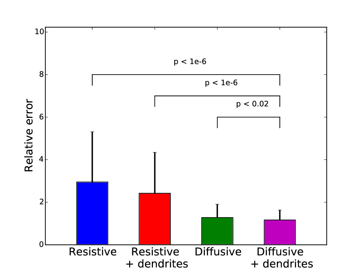
Figure 5: Average fitting error of the four models. The figure shows the average goodness of fit for 4 different models investigated: Resistive, Resistive with Dendrite, Diffusive, and Diffusive with Dendrite. The error bars are standard deviations of fitting errors. The testing variable used to compare the quality of these fits takes into account their different number of variables. Of all models, the diffusive models give the smallest error in all cases tested. The best fit is provided by the diffusive model with dendrite, although only marginally better than the diffusive model in a single-compartment model.

5. The F cumulative distribution function (fcdf) allows us to compute the likelihood of $H_{0}$ (Fig. 5):

$$p=1-fcdf(F)$$

If p < $\alpha$, we reject the null hypothesis: the diffusive model with dendrites is significantly better than the other model, and this can not be explained by the surplus of parameters alone.

Computational models using the measured impedances

Two types of models were used to test possible consequences of the measurements. First, we used a model of the genesis of the extracellular potential. To this end, a current waveform corresponding to the total membrane current generated $I_{AP}(t)$ by an action potential was computed from the Hodgkin-Huxley model in the NEURON simulation environment [27]. This current waveform was used as a current source to calculate the extracellular potential, using a formalism that is valid for any extracellular impedance. We calculated the extracellular potential by using the impedance measurements made in the present paper. According to 2, we have:

$$Z_{e}(\omega)=\frac{A+iB}{1+\sqrt{i\ \omega/\omega_{W}}}~{},$$ (10)

where $A=151\times 10^{6}\Omega$, $B=2.54\times 10^{6}\Omega$ and $\omega_{W}=335~{}rad.s^{-1}$ for a distance of a few $\mu m$. The extracellular potential $V(t)$ was calculated using the convolution:

$$V(t)=\int_{-\infty}^{+\infty}\bar{Z}_{e}(t-\tau)I_{AP}(\tau)d\tau~{},$$ (11)

where $\bar{Z}_{e}(t)$ is the inverse Fourier transform of $Z_{e}(\omega)$.

Second, we simulated a ball-and-stick model using the generalized cable equation [28] (see Eq. 5).

A zero-mean Gaussian white-noise current waveform was injected into the dendrite, and the generalized cable was used to compute the membrane potential in dendrites and in the soma (see details of the methods in ref. [28]).

Results

We start by outlining the measurement paradigm and the notion of global intracellular impedance, then we successively describe the results obtained in vitro and in vivo. Finally, we illustrate consequences of these findings on two fundamental properties, the genesis of extracellular potentials, and the voltage attenuation along neuronal dendrites.

The global intracellular impedance

Here, we explore the hypothesis that the extracellular impedance is fundamentally different if measured in natural conditions where the interface between the neuronal membrane and extracellular medium is respected, compared to metal electrodes, which rely on an artificial metal-medium interface. In natural conditions, the neuronal membrane’s interface with the medium involves the opening/closing of ion channels, ionic concentration differences and ionic diffusion, whereas metal electrodes involve a different type of ion exchange with the medium, which consists of a chemical reaction between the metal and the ions in the medium. To measure the impedance in natural conditions, it is therefore necessary to use an intact neuron as the interface with the medium, to respect the correct ionic exchange conditions. To do this, we performed whole-cell patch-clamp recordings, using neurons as natural current sources in the surrounding medium.

This measurement paradigm is illustrated in Fig. 1A-B and consists of a whole-cell patch-clamp recording coupled to a micropipette measuring the potential in the extracellular medium close to the recorded neuron, in vitro (Fig. 1A) or in vivo (Fig. 1B). In all cases, the recorded neuron is driven by current injection and serves as a natural current source in the medium. In this configuration, relating the signals of the two electrodes gives a direct access to the extracellular impedance, as shown by the equivalent circuits (Fig. 1C).

According to this equivalent circuit, we have:

$$V_{intra}=Z_{eq}.i^{g}~{},$$ (12)

where $i^{g}$ is the generalized current injected by the patch-clamp electrode. The use of the generalized current is essential here because it is the only current that is conserved if the media have arbitrarily complex impedances [28], and therefore abides to Kirchhoff’s current laws in this general case. Note that the current provided by the current generator is also a generalized current because capacitive or non-resistive effects are negligible in modern generators.

In contrast, the conservation of the classic “free-charge current” would apply only with resistive impedances. The previous equation gives, for the left circuit (single-compartment cell):

$$Z_{eq}(\omega)=Z_{i}+\frac{R_{m}}{1+i\omega\tau_{m}}+Z_{e}~{},$$ (13)

and for the right circuit (cell consisting of a soma and an equivalent dendrite):

$$Z_{eq}(\omega)=Z_{i}+\frac{(Z_{s}+Z_{e})Z_{d}}{Z_{s}+Z_{e}+Z_{d}}~{},$$ (14)

where $Z_{eq}$ is the equivalent impedance of each of the two circuits, $Z_{i}$ and $Z_{e}$ are the macroscopic impedances of the cytosol and the extracellular medium, respectively. $R_{m}$ is the global input resistance of the cell and $\tau_{m}$ is the global membrane time constant (left circuit); $Z_{s}=\frac{R_{m}}{1+i\omega\tau_{m}}$ is the impedance of the soma membrane (right circuit), $Z_{d}$ is the input impedance of an equivalent dendrite, as seen by the soma, including the extracellular medium surrounding it.

In the standard model, $Z_{i}$ and $Z_{e}$ are usually modeled by a lumped and resistive impedance. In the following, $Z_{eq}$ will be called the “global intracellular impedance” of the circuit, because in such a recording configuration the neuron acts as a current source in the brain tissue. It represents the impedance of the system as seen by the intracellular side of the neuron.

$Z_{e}$ is the impedance of the extracellular medium as seen by the neuron (extracellular component of the intracellularly-measured global impedance). We will test here if the latter impedance is negligible or constant, as usually assumed. We will consider resistive and diffusive versions of this impedance and check which one better fits the data.

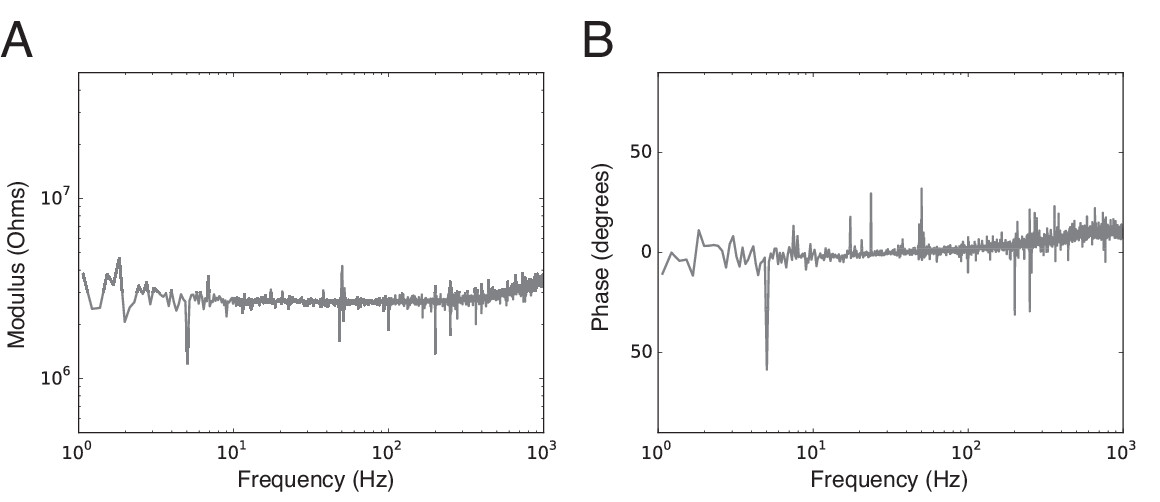
Figure 3: Impedance of a silver-silver chloride electrode inserted in a typical ($\approx 3~{}M\Omega$) patch pipette, measured in ACSF. Left: modulus (Ohms), right: phase (degrees).

$Z_{i}$ includes the impedance of the interface between the tip of the electrode and the intracellular medium. This interface will be different in whole-cell patch or sharp-electrode recording configurations, because of the location and impedance of the pipettes themselves. So, the interpretation of the measured impedances may be different in sharp-electrode and whole-cell recordings, and we indeed have observed such differences (not shown here). In particular, we made sure that the interface of the silver-silver chloride electrodes, used for patching and as a reference, does not contribute significantly to the equivalent impedance: it is negligible compared to other impedances in the circuit and has little frequency dependence between 1 and 1000 Hz (see Fig. 3).

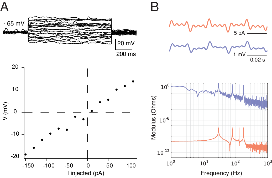
Figure 4: Linearity in temporal and frequency space. A: injection of hyperpolarizing and depolarizing pulses in a cortical neuron patched in vivo, around resting membrane potential. The V-I relation indicated is roughly linear in this subthreshold range. B: Sine waves of current with four different frequencies were injected simultaneously in a patched neuron in vivo (top, red curve). The voltage was recorded (top, blue curve). The modulus of the Fourier Transform of both signals is shown here, as a function of frequency (Hz): current in red (A), voltage in blue (V). The frequencies corresponding to the peaks on both signals illustrate the linearity in frequency of the system, here tested between 1 and 1000 Hz.

In order to measure $Z_{eq}$, we injected a current intracellularly, and measured the intracellular potential $V_{intra}$ with respect to a reference. Ideally, this reference is a micropipette in the extracellular medium (V_LFP; see scheme in Fig. 1A). In the in vivo experiments, the reference was a silver electrode inserted in the contralateral somatosensory cortex as in Fig. 1B. For subthreshold currents, the system can be considered linear in frequency: injecting current at an arbitrary frequency yields voltage variations only at that frequency (see Appendix 2 in Supplementary Material). This linearity of the system is illustrated in Fig. 4. First, for the subthreshold range of $V_{m}$ considered, the membrane V-I relation is linear (Fig. 4A). Second, a combination of four sine-wave currents of fixed frequency generate $V_{m}$ variations that have strictly the same frequencies (Fig. 4B), showing that the linear approximation is valid: sine waves appear as sharp spectral lines in Fourier space, two orders of magnitude above baseline. Thus, there seems to be no significant impact of non-linear membrane ion channels on the recordings. Indeed, no action potentials were present in the recordings analyzed here.

We used two protocols of current injection, either injection of a series of sinusoidal currents of different fixed frequencies (6 to 926 Hz), or injection of a broad-band (white noise) current, with a flat spectrum between 1 and 10 kHz. In this case, several instances of the same noisy current trace were injected in the cell (“frozen noise” protocol), which allowed us to take average and increase the signal-to-noise ratio of the measurements. This is particularly useful in vivo, to limit the contamination of the measurement by spontaneous synaptic activity, which can be very strong in vivo.

In vitro measurements of the global intracellular impedance

Measurements were first performed in vitro by using an experimental setup consisting of a whole-cell patch-clamp recording of a neuron, together with an extracellular recording in the nearby tissue in the cortical slice (see Fig. 2A). Using this recording configuration, we computed the global intracellular impedance ($Z_{eq}$ in Eq. 12; see Materials and Methods) by using either white-noise current injection, or injected sinusoidal currents. The results of a representative cell ($N=31$) is shown in Fig. 2B-C. Both the modulus amplitude and Fourier phase of the impedance are represented. The colored curves in Fig. 2B-C show the best fits of different models to the experimental data. One can see that the purely resistive model (RC membrane + resistive extracellular medium, blue curves) does not capture the data. We read from equation 1 that $\lvert Z_{eq}(\omega)\rvert$ scales as $1/\omega$ in the resistive model, which corresponds to a slope of -1, while the experimental modulus yields a slope of $-0.5\pm 0.1$ (Fig. 2D). The resistive model has a phase similar to arctan($k\omega$) with a minimum of about -90 degrees at high frequencies, which contrasts with the -50 degrees observed in the data (Fig. 2E).

So frequency dependence is clearly different from that predicted by the RC-circuit membrane model. The best fits of a model taking into account ionic diffusion [22] can account significantly better for most of this frequency dependance in different cells (green curves; see also Fig. 5). In particular, the $1/\sqrt{\omega}$ frequency scaling predicted by the diffusive model (equation 3), corresponds to the actually observed -0.5 slope of the modulus. The phase modulations can also be remarkably well captured by the diffusive model.

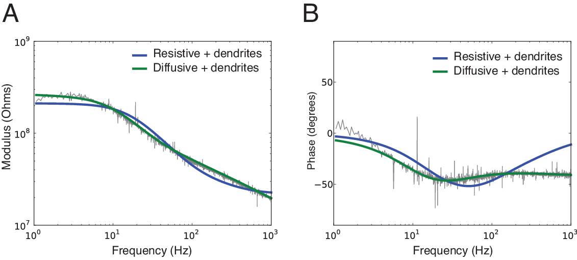
Figure 6: Dendritic contribution to the global intracellular impedance of a cortical neuron recorded in vitro (current clamp). Same arrangement of panels as in fig. 2, except that the different curves show the best fit of two models to the experimental data (blue: resistive, green: diffusive), both models included an equivalent dendritic compartment. Parameters of the models: i) Resistive: ${\color[rgb]{0,0,0.65}R_{s}}=~{}240M\Omega$, ${\color[rgb]{0,0,0.65}C_{s}}=37~{}pF$, ${\color[rgb]{0,0,0.65}R_{e}}=21~{}M\Omega$, ${\color[rgb]{0,0,0.65}l_{dend}=390~{}\mu m}$; ii) Diffusive: ${\color[rgb]{0,0,0.65}R_{s}}=150~{}M\Omega$, ${\color[rgb]{0,0,0.65}C_{s}}=~{}89pF$, ${\color[rgb]{0,0,0.65}A}=~{}130M\Omega$, ${\color[rgb]{0,0,0.65}B}=-12~{}M\Omega$, ${\color[rgb]{0,0,0.65}f_{W}}=30~{}Hz$, ${\color[rgb]{0,0,0.65}l_{dend}=12~{}\mu m}$. ${\color[rgb]{0,0,0.65}A}$, ${\color[rgb]{0,0,0.65}B}$ and ${\color[rgb]{0,0,0.65}f_{W}}$ are parameters of the diffusive impedance scaling respectively its amplitude, phase, and cutoff frequency.

We also tested the possible influence of dendrites, by including an equivalent dendritic compartment in the circuit (Fig. 1C, right). This addition could not rescue the resistive model, which was still unable to match the observations (Fig. 6). We have considered variations of dendritic parameters, including very long dendritic segments, different axial and leak conductances, and did not see any significant improvement by the addition of dendrites. In the diffusive model, taking the dendrites in account only enhanced marginally the agreement between experimental and theoretical curves. Statistical analysis showed that the improvement in quality from the resistive to the diffusive model was significant, and not only due to a higher number of parameters. Furthermore, the apparent smaller number of parameters in resistive models can come from hidden assumptions, such as homogeneity and low resistivity of the extracellular medium.

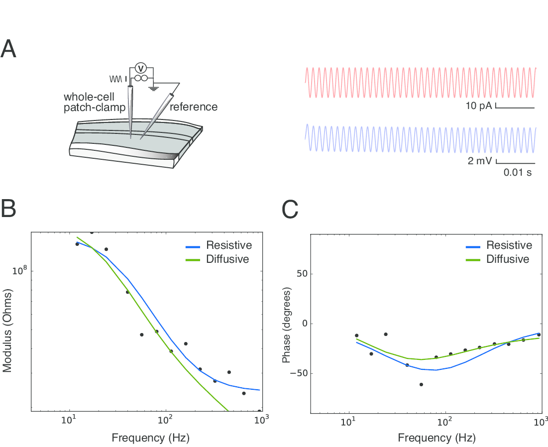
Figure 7: Global intracellular impedance measurements of a striatal neuron recorded in vitro (current clamp) and stimulated with sinusoid inputs from 6 to 926 Hz. A: sine waves of current (top, red; minimum 25 samples and 20 cycles per sample) were injected in patched neurons while recording the intracellular potential (top, in blue; 16.7 kHz sampling). B: modulus of $Z_{eq}$ (log scale) represented as a function of frequency ($log_{10}(f)$), for sine wave current injection (600 pA amplitude). C: Fourier phase of $Z_{eq}$ in the same experiment. Parameters of the models: i) Resistive: ${\color[rgb]{0,0,0.65}R_{m}}=120~{}M\Omega$, ${\color[rgb]{0,0,0.65}C_{m}}=~{}46pF$, ${\color[rgb]{0,0,0.65}R_{e}}=28~{}M\Omega$; ii) Diffusive: ${\color[rgb]{0,0,0.65}R_{m}}=130~{}M\Omega$, ${\color[rgb]{0,0,0.65}C_{m}}=59~{}pF$, ${\color[rgb]{0,0,0.65}A}=58M\Omega$, ${\color[rgb]{0,0,0.65}B}=43~{}M\Omega$, ${\color[rgb]{0,0,0.65}f_{W}}=50~{}Hz$. Representative of $N=18$ cells.

These results were replicated in striatal neurons using purely sinusoidal input currents from 6 to 926 Hz (see Fig. 7, $N=18$), thereby confirming that the global shape of the global cell impedance does not depend on the stimulation protocol. In addition, we tested a capacitive (RC) model of the extracellular space, but this model did not account for the modulus and the phase modulations (it was the worst fit of all models tested – not shown).

We also checked whether the quality of seals could affect the global intracellular impedance measurements. Indeed, if the cell membrane is bypassed, the impedance is not measured anymore through the natural interface of a neuron membrane. The average of neurons with good seals (> 1 G$\Omega$) yields a slope of $-0.5\pm 0.1$ (see fig. 2D); in comparison, cells with extremely poor seals (e.g. 200 M$\Omega$, not included in the data shown here) yielded a flatter impedance, with a slope between 0 and -0.3. This can be easily explained by replacing $Z_{RC}$ by a resistance in the expression of $Z_{eq}$.

Finally, we checked whether part of the observed frequency dependence could be due to the recording pipette. We found that the frequency dependence of the patching pipette and silver-silver chloride electrode is negligible in ACSF (Fig. 3). These measurements show that the observed frequency dependence of the impedance cannnot be attributed to the silver electrode interface, and probably stems from the properties of the extracellular medium.

Global intracellular impedance in vivo

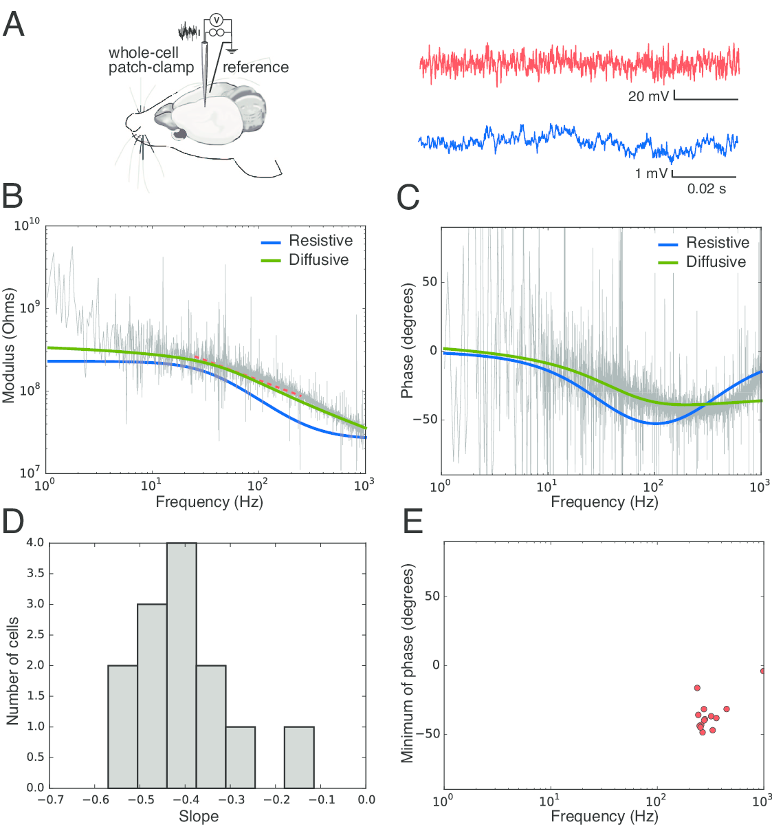
Figure 8: Global intracellular impedance of cortical neurons recorded in vivo in current-clamp. A: Scheme of the recording configuration, with a similar representation as in Fig. 2A, but performed in rat somatosensory cortex in vivo (with a contralateral reference electrode), using white noise current injection. For these experiments, we injected 20 times the same gaussian white noise current trace (top, in red), recorded at 20 kHz and averaged the intracellular potential (top, in blue). We calculated the impedance seen by the neuron. B: Modulus of the impedance obtained, as a function of frequency. C: Phase of the impedance. Parameters of the models: i) Resistive: ${\color[rgb]{0,0,0.65}R_{m}}=230~{}M\Omega$, ${\color[rgb]{0,0,0.65}C_{m}}=28~{}pF$, ${\color[rgb]{0,0,0.65}R_{e}}=29~{}M\Omega$; ii) Diffusive: ${\color[rgb]{0,0,0.65}R_{m}}=100~{}M\Omega$, ${\color[rgb]{0,0,0.65}C_{m}}=~{}21pF$, ${\color[rgb]{0,0,0.65}A}=250~{}M\Omega$, ${\color[rgb]{0,0,0.65}B}=24~{}M\Omega$, ${\color[rgb]{0,0,0.65}f_{W}}=20~{}Hz$ Representative of $N=18$ cells. D: Distribution of the slopes of $Z_{eq}$ fitted between 25 and 250 Hz (linear fit, red dashed lines on the figures). E: Coordinates of the minima of the Fourier phases for each cell.

In a second set of experiments, the measurements were performed in vivo with whole-cell patch-clamp recordings of pyramidal cells of the somatosensory cortex, layer V (see scheme in Fig. 8A and details in Materials and Methods). Similarly to Fig. 2, the modulus and phase of the impedance were estimated by white noise current injection (Fig. 8B-C). Although the data display a high degree of noise (due to spontaneous synaptic inputs in vivo), they were in qualitative agreement with in vitro results on $N=18$ cells. The resistive model did not capture the modulus amplitude, nor the phase of the global intracellular impedance of the neuron. The diffusive model was able to capture the essential variations, both in amplitude (modulus) and phase domain. Similar to in vitro measurements, the modulus yields a slope of $-0.4\pm 0.1$ (Fig. 8D), and a minimum phase around -50 degrees (Fig. 8E), which significantly deviate from predictions of a resistive model.

As in the in vitro experiments, the addition of an equivalent dendritic compartment did not improve these differences. The resistive model with dendrites was also unable to account for the measurements, while the diffusive model provided acceptable fits to the data.

One must keep in mind that the in vivo measurements were made in the presence of low-frequency spontaneous activity, typical of anesthetized states. This “synaptic bombardment” probably explains the mismatch of all impedance models at low frequencies in vivo. Such a mismatch was not present in vitro.

Possible consequences of these measurements

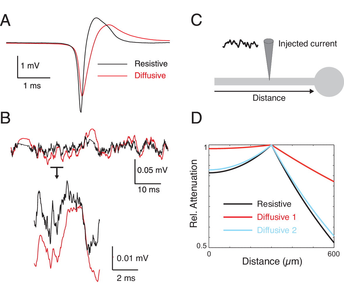
Figure 9: Consequences of the diffusive nature of the extracellular medium. A. Simulation of LFP in the extracellular medium (10 $\mu$m from the soma) following injection of current following a spike waveform. The panel compares the extracellular spike obtained for a resistive medium (black), compared to a diffusive medium (red), where the filtering is evident. B. Same simulation as in A, but using injection of the combined current of noisy excitatory and inhibitory (subthreshold) inputs. In this case, the LFP obtained in a resistive and diffusive medium are also differentially filtered. C. Scheme of a ball-and-stick neuron model where a noisy current waveform was injected in the middle of the dendrite. D. Relative voltage attenuation profile obtained (at 5Hz) when the neuron is simulated in resistive (black) or diffusive (red, blue) media. Two diffusive configurations were simulated, Diffusive 1: diffusive intracellular and extracellular media (red curves); Diffusive 2: diffusive extracellular medium with resistive intracellular medium (blue curves). Using diffusive media results in a reduced voltage attenuation. In all cases, the resistive or diffusive media were simulated using the best fits to the impedances measured in vitro.

Finally, to evaluate possible consequences of these measurements, we have considered two situations where the extracellular impedance can have strong consequences. A first consequence is the fact that the diffusive nature of the medium will necessarily impose frequency filtering properties on extracellular potentials, which affects measurements made with extracellular electrodes. To illustrate this point, we simulated extracellular potentials generated by a current source corresponding to the total membrane current generated by an action potential (using the Hodgkin-Huxley model). We then calculated the extracellular potential at a distance from this current source, using either a resistive model, or a diffusive model (Fig. 9A). Interestingly, one can see that the extracellular signature of the spike has a slower time course in diffusive conditions. A similar situation was also simulated using subthreshold noisy excitatory and inhibitory synaptic activity (Fig. 9B). In both cases, the nature of the medium influences the shape and propagation of the local field potential (LFP), for both extracellular spikes and LFP resulting from synaptic activity.

A second possible consequence is on the cable properties of neurons. This point was illustrated by simulating a ball-and-stick model subject to injection of a noisy current waveform in the dendritic cable (Fig. 9C). As shown in Fig. 9D, the attenuation of the voltage along the dendrite can be drastically different in a diffusive medium compared to a resistive medium, as noted previously [28]. Including a diffusive extracellular medium reduced voltage attenuation (Fig. 9D, blue curve), but this reduction was the strongest when both intracellular and extracellular media were diffusive (red cuves). Thus, the nature of the medium will also influence the shape and propagation of potentials in dendrites.

Discussion

We have provided here the first experimental measurements of the impedance of the extracellular medium, in natural conditions, in vitro and in vivo. We found that, not only the estimated extracellular impedance is higher compared to traditional metal-electrode measurements, but it is also more frequency dependent. The standard model, considering the medium as resistive, can account for metal electrode measurements, but not for natural impedance measurements. In contrast, we found that a diffusive model can account for most measurements, both in modulus amplitude and in phase. We also checked whether the inclusion of dendrites could affect these conclusions, but it did not qualitatively change these results.

It is noteworthy that the present measurements are made between a neuron, and a reference electrode in the nearby tissue. Therefore, the current presumably flows in the entire tissue, and thus, the impedance measured can be considered “macroscopic”. From the different experiments realized here, we estimate that the impedance is determined by the region close to the membrane, within distances of the order of hundreds of microns in cerebral cortex.

The apparent inconsistency with the previous metal-electrode measurements can be resolved by considering that each kind of electrode has a specific interface and impedance, depending on its physical nature [7]. Classical impedance measurement studies tackle this problem offline with a normalization by a measure in saline [3, 10], online by removing the effect of the interface using the saturation due to large currents [5], or by minimizing the interface [29, 30]. In physiological conditions, neurons have an electrical interface with the extracellular medium, as a part of their normal environment. This interface should therefore not be removed when using neurons to evaluate the impedance of the extracellular medium, as it is one of the keys to explaining the electric field produced by an active cell.

The system presented here deals with the usual problems of electrode recordings (see ref. [29]) in unusual ways, which solves some classical issues but raises new interrogations. First, the electrode – or neuron – must be standardized. It is remarkable to see that, despite the considerable cell-to-cell variability in size or morphology, we obtained here very consistent measurements, with very similar amplitude and phase profiles from cell to cell. These measurements can be captured with accuracy with a limited number of parameters, most of which are well known ($R_{m}$, $C_{m}$…). How the cellular morphology influences these results, and why this influence seems so small, constitute interesting subjects for future extensions of the present work. Second, the spatial scale concerned by potential measurement and current injection is a grey area in the litterature (see ref. [31]). We believe that the scale of a single neuron may be as relevant as the tip of traditional recording electrodes, of arbitrary size and position in an inhomogenous medium, which can affect recordings significantly [14]. Third, the interface of the electrode and its behavior must be linear and well understood within the measurement range, which we discussed previously. Provided the system is operated with all necessary precautions, linearity is maintained (Fig. 4); the path of the injected currents in neuron compartments does not seem to be a crucial matter (Fig. 14) and injected currents splitting between different forms (free or bound charges, electric flux…) is not a problem within the generalized current formalism. Furthermore, the traditional 4-electrode setup is designed to separate voltage recording from possible filtering by the interface generated when injecting current [30]. In the system presented here, the silver-silver chloride wire has a very resistive interface (Fig. 3) and is negligible with respect to the main, relevant interface of the recorded neuron.

A possible explanation for the prominent role of ionic diffusion is that when a neuron acts as a current source, the electric field lines will not, in general, match the complex geometry of the extracellular medium. The trajectory of ions would thus be affected by obstacles such as cells and fibers [14], which would yield local variations in ionic concentrations. Ionic diffusion would therefore exert an important force on ions in the extracellular medium. A linear approximation of this phenomenon allows one to model this contribution by a Warburg-type impedance, scaling as $\frac{1}{\sqrt{\omega}}$. In addition, ionic diffusion is involved in membrane potential changes, and participates as well to maintaining the Debye layer surrounding the membrane [32]. Taken together, these factors could explain why the present measurements are in such good agreement with the diffusive model.

Despite this agreement, the participation of diffusive phenomena can vary with age and experimental conditions. As the brain gets older, the extracellular volume fraction shrinks, which could make ionic diffusion even stronger and thus reinforce the Warburg component of the natural impedance. Furthermore, in vivo tissue may be more confined than in vitro, with a similar result on the importance of ionic diffusion. One can thus reasonably expect $Z_{W}$ to be stronger in P30 rats in vivo ($N=18$) than in P12-16 mice in vitro ($N=31$). Indeed, the components $A$ and $B$ of $Z_{W}$ are significantly stronger in vivo in P30 rats than in vitro in P12-16 mice (comparing the medians $\pm$ the standard error of the mean: resp. $96\pm 12~{}M\Omega$ vs $183\pm 16~{}M\Omega$ for $A$ and $6.6\pm 2.7~{}M\Omega$ vs $28\pm 3.7~{}M\Omega$ for $B$). Thus, the age of the subject and type of recording need to be taken into account when using measured values of the natural impedance. In particular, it may lead to an underestimation of $Z_{W}$ in this paper, because we mainly focused on in vitro recordings in young mice; our conclusions on the importance of ionic diffusion are thus rather conservative. It is noteworthy that in between these two sets of observations, the Warburg frequency remains the same : $43\pm 3~{}Hz$ in vitro vs $42\pm 3~{}Hz$ in vivo.

Our results do not disqualify the previous measurements, but are complementary. We suggest that for all cases where the current sources are generated by natural conditions (i.e., by neurons), the global intracellular impedance should be used. This is the case for example when analyzing the LFP signal, or with Current Source Density (CSD) analysis. In cases where a metal electrode is used to inject current, the metal-electrode impedance would be relevant, for example, in Deep Brain Stimulation paradigms.

Note that, although the diffusive model accounts very well for the modulus and phase variations of the global intracellular impedance, there exists small deviations, in particular at high frequencies. The latter may be due to a number of phenomena, including variability in neuron geometry or limitations of the linear approximations used here. The existence of “shunts” due to the liquid around the electrodes is also not to be excluded. Further studies should be designed to identify the contribution of such factors, e.g. pharmacological inactivation of nonlinear channels. Two arguments suggest that the present formalism is satisfactory, the strong reproducibility of results across 31 recorded neurons in vitro, despite intrinsic biological variability, and the coherence between the diffusive model and experimental data.

The exact boundaries of the domain where these results apply are still to be determined. For example, in figure 9 we are extrapolating into a nonlinear region to make implications about the shape of the action potential. We think this extrapolation is acceptable because non-linear behavior is mostly happening in the highest frequencies, barely overlapping with the LFP frequency range (see also Appendix 2 in Supplementary Material), but one should be aware of that caveat.

Finally, using computational models, we illustrated consequences of the medium non-resistivity on extracellular and intracellular potentials. A number of fundamental theoretical equations used in neuroscience, such as CSD analysis [33], or neuronal cable equations [25, 26] were originally derived under the assumption that the extracellular medium is resistive. If the medium is non-resistive, these equations are not valid anymore and must be generalized. Attempts for such generalizations were proposed recently for CSD analysis [22] and cable equations [28], but they were not constrained by measurements. The simulations provided here show that including a diffusive impedance based on the present measurements has significant consequences, for both extracellular potentials, and for the electrotonic properties of neurons. The shape of the extracellular spike may be affected by the nature of the medium (Fig. 9A), assuming that one can extrapolate the present results to the nonlinear region of the $V_{m}$. This shows that the sharpness of the extracellular spike may be influenced by the properties of the medium, which constitutes another factor that could complicate the identification of neurons from spike shape. The dendritic attenuation is also reduced in the presence of a diffusive medium (Fig. 9D-E), as shown previously [28]. Extrapolating these results, it seems that the sources estimated by CSD analysis, could greatly be affected by the nature of the extracellular medium, which constitutes a direct extension of the present study. Similarly, source reconstruction methods from the EEG, are also likely to be affected by the nature of the medium, and thus, these methods may need to be re-evaluated as well.

Author contributions

JMG, SV, MN, PP and TB performed the in vitro experiments. LV performed the in vivo experiments. Analyses were designed by AD and CB and were performed by JMG, CB, MN, VK and AD. AD, TB and LV cosupervised the work.

Acknowledgments

Research supported by the CNRS, the Paris-Saclay excellence network (IDEX), INSERM, Collège de France, Fondation Brou de Laurière, Fondation Roger de Spoelberch, French Ministry of Research, the ANR (Complex-V1 project), the Eiffel excellency grants program, and the European Community (BrainScales FP7-269921, Magnetrodes FP7-600730 and the Human Brain Project FP7-604102). We thank Sylvie Perez for technical assistance with the in vivo experiments.

Tables

Model type	Resistive	Diffusive
No dendrite	$R_{m}$, $C_{m}$, $R_{e}$	$R_{m}$, $C_{m}$, $A$, $B$, $f_{W}$
Dendrite	$R_{s}$, $C_{s}$, $R_{e}$, $l_{d}$	$R_{s}$, $C_{s}$, $A$, $B$, $f_{W}$, $l_{d}$

Table 1: Parameters used for the four models. $l_{d}$ is the length of the dendritic compartment. $R_{e}$ is the extracellular resistance.

Model type	$Z_{i}=z_{i}l_{s}$	$Z_{e}$	$z_{e}^{(m)}$	$\kappa_{\lambda}^{2}$
Standard	$r_{i}l_{s}$	negligible	negligible	$\frac{r_{i}}{r_{m}}(1+i\omega\tau_{m})$
Diffusive	$\frac{r_{i}}{(1+i)\sqrt{\omega}}l_{s}$	$\frac{A+iB}{1+\sqrt{i\omega/\omega_{W}}}$	$\frac{0.5\tau_{m}}{2\pi aC_{m}(1+i)\sqrt{\omega}}$	$\frac{z_{i}(1+i\omega\tau_{m})}{r_{m}[1+\frac{z_{e}^{(m)}}{r_{m}}(1+i\omega\tau_{m}]}$

Table 2: Intermediate variables. $Z_{i}$ and $Z_{e}$ are respectively the intracellular and extracellular impedances, $z_{e}^{(m)}$ is the input resistance of the extracellular medium seen by the dendrite (in $\Omega/m$), $\kappa_{\lambda}$ is the cable parameter of the system. Constants: $r_{i}$ and $r_{e}$ are the linear density of resistance in the cytoplasm and extracellular medium (estimated to $28\times 10^{9}$ and $18\times 10^{9}$ $\Omega/m$), $z_{i}$ is the linear density of impedance in the dendrite, $l_{s}$ and $l_{d}$ are the length of the soma and dendrite, $a$ is the diameter of the dendrite, $\tau_{m}$ is the time constant of the membrane ($\sim$10 ms), $C_{m}$ is the specific membrane capacitance ($10^{-2}~{}F/m^{2}$). We also have $r_{m}=\tau_{m}/2\pi a_{m}C_{m}$, where $1/r_{m}$ is the linear density of membrane conductance (S/m).

Figures

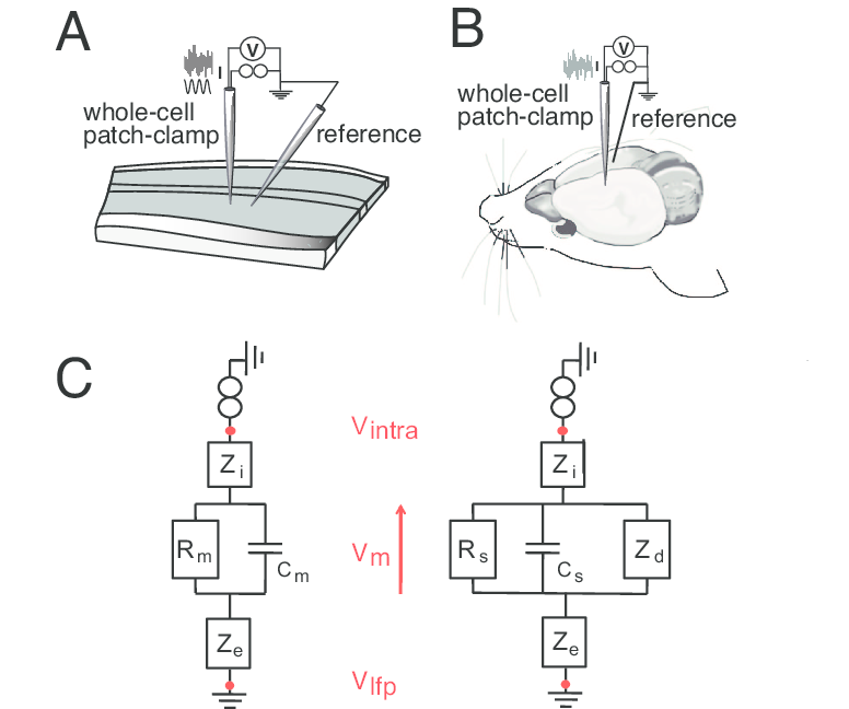
Figure 1: Scheme of the experimental setup for measuring the global intracellular impedance. A-B: Placement of electrodes in vitro and in vivo. In each case, a cell is recorded in patch-clamp whole-cell configuration using a micropipette, where the reference electrode is a micropipette located in the extracellular medium at a short distance from the recording (A), or a silver wire in the contralateral hemisphere (B). C: Equivalent circuits corresponding to this experimental setup, in two different configurations: the cell is either considered as a single compartment (left), or with dendrites (right), resulting in a slightly more complicated circuit. The membrane is modeled as a RC-circuit, where $R_{m}$ and $C_{m}$ are the global membrane resistance and capacitance of the cell (left), respectively, or $R_{s}$ and $C_{s}$ are the resistance and capacitance of the somatic membrane (right). $Z_{i}$ is the macroscopic intracellular impedance (including the electrode-cytosol interface), and $Z_{e}$ is the macroscopic extracellular impedance. In the resistive models, $Z_{e}$ is modeled as a simple resistance $R_{e}$; in the diffusive models, it is a function of three parameters ($A$, $B$ and $k$, respectively scaling the modulus, phase and cutoff frequency of the diffusive impedance; see Materials and Methods). In the right circuit, $Z_{d}$ is the equivalent input impedance of the dendritic tree seen by the soma; it is a function of $l_{d}$, the equivalent length of the dendritic tree. In both circuits, $V_{intra}$ represents the intracellular potential, and $V_{lfp}$ the potential in extracellular space.

Supplementary material

Appendix A Appendix 1: Integrating the global intracellular impedance in models

In this appendix, we relate the impedance $z_{e}^{(m)}$ in the generalized cable, to the impedance measurements reported in the present paper. In the generalized cable [28], the extracellular impedance was modeled by parameter $z_{e}^{(m)}$. Starting from the expression of the extracellular impedance,

$$Z_{e}=\frac{z_{e}^{(m)}}{A_{soma}}=\frac{z_{e}^{(m)}}{4\pi R_{soma}}$$ (A.1)

and condisering a single-compartment model, according to Eq. 13, we can write

$$z_{e}^{(m)}\approx A_{soma}Z_{e}=A_{soma}[Z_{eq}(\omega)-\frac{R_{m}}{1+i\omega\tau_{m}}]~{}.$$ (A.2)

Thus, by assuming a typical somatic membrane area, we can estimate $Z_{e}$, and thus also estimate $z_{e}^{(m)}$. The other parameters, $R_{m}$, $\tau_{m}$, $Z_{eq}$, can also be estimated from the present measurements.

Appendix B Appendix 2: Establishing the linearity of the system

In this Appendix, we explain how to determine the linearity of the system, in temporal and frequency space.

B.1 Linearity in Fourier frequency space

In the Fourier frequency domain, the experiments show that the ratio $\Delta V(\omega)~{}/~{}I^{g}(\omega)$ is a bounded function for variations around the resting membrane potential. In these conditions, a sinusoid in current gives a sinusoid voltage with the same frequency, and with no additional peak in the spectrum. This is true for relatively small variations (a few millivolts), keeping the membrane far away from spike threshold. As shown in Fig. 1D, a combination of sine-wave currents generates a voltage power spectrum with peaks at the same position in frequency, and where no additional peak or harmonics appear. We can say that in this case, the membrane potential of the neuron is linear in Fourier frequency space. This implies that each component of this system in this space is also linear, and in particular, the V-I relation of ion channels in the membrane are linear, because the membrane capacitance is approximately constant (White, 1970). This is an expression of Ohm’s law, in which the ion channels are equivalent to a resistor, with no voltage-dependent effects (see Section B.2).

To demonstrate this, we note that the ratio between $V$ and $I^{g}$ is a continuous bounded function in Fourier frequency space, with the constraint $V(0)=g(\omega,0)=0$ for $\omega\neq 0$ (the latter condition means that the neuron is at rest when the transmembrane current is zero). In these conditions, we have

$$V(\omega)=g(\omega,I^{g}(\omega))~{}.$$ (B.1)

We can develop $g$ in Taylor series relative to the current, because the domain of definition of $g$ is necessarily compact in experimental situations. Consequently, we can write:

$$\begin{array}[]{ccl}\Delta V(\omega)=V(\omega)-V(0)&=&\frac{\partial g}{\partial I^{g}}(\omega,0)I^{g}(\omega)+\frac{1}{2!}\frac{\partial^{2}g}{\partial I^{g2}}(\omega,0)I^{g2}(\omega)+\cdots{}\\ \\ \\ &=&b_{1}(\omega)I^{g}(\omega)+b_{2}(\omega)I^{g2}(\omega)+\cdots~{}.\end{array}$$ (B.2)

The impedance is then given by:

$$Z(\omega)=\frac{\Delta V(\omega)}{I^{g}(\omega)}=b_{1}(\omega)+b_{2}(\omega)I^{g}(\omega)+\cdots~{}.$$ (B.3)

We can see that, if the spectrum $I(\omega)$ is a discrete Fourier spectrum composed of Dirac delta functions, then $Z(\omega)$ cannot be a bounded function when $b_{n}\neq 0$ for $n>1$. Thus, we obtain

$$\Delta V{\omega}=b_{1}(\omega)I^{g}(\omega)$$ (B.4)

when the ratio $V(\omega)/I^{g}(\omega)$ is a bounded function. In other words, the system is necessarily linear in Frequency space because the V-I relation does not depend on the current amplitude. Note that this independence is only true in the absence of voltage-dependent conductances, so it can apply to the subthreshold range, near the resting membrane potential. Such a linear dependence also implies that the position of spectral lines is necessarily identical between $V(\omega)$ and $I^{g}(\omega)$.

B.2 Linearity of traditional V-I curves

We now address the question of whether the V-I relation of ion channels is linear when these channels are linear in Fourier frequency space, and vice-versa.

In general, for a membrane containing ion channels, we have:

$$V=f(I)~{},$$ (B.5)

with V = f(0)= cst for zero current (resting membrane potential).

We can approximate $V$ as precise as we want using a polynomial of the current, because $V$ is necessarily a continuous function of this variable since the electric field is finite ($\vec{E}=-\nabla V$). This is by virtue of the Stone-Weierstrass theorem [34], which states that every continuous function defined over a closed and bounded domain, can be approximated as close as we want by a polynomial. Thus, for a given population of ion channels, we can write

$$\Delta V(t)=V(t)-V(0)=a_{1}I+a_{2}I^{2}+\cdots.$$ (B.6)

If we express $I$ as $I(t)=e^{i\omega t}$, we obtain

$$\Delta V(t)=a_{1}e^{i\omega t}+a_{2}e^{2i\omega t}+\cdots$$ (B.7)

such that the Fourier transform of the variations of $V$ around $V(0)$ generally gives a spectrum very different from that of the current. Indeed, applying the Fourier transform gives

$$\Delta V(\omega)=a_{1}~{}\delta(\omega^{\prime}-\omega)+a_{2}~{}\delta(\omega^{\prime}-2\omega)+\cdots$$ (B.8)

Thus, it is necessary that $\forall n>1$ we have $a_{n}=0$ if we want that the position of the spectral lines of $\Delta V(\omega)$ is the same as that of $I(\omega)$.

Moreover, it is evident that if the function $f$ is linear, then the position of the spectral lines of $\Delta V(\omega)$ is the same as that of $I(\omega)$.

Thus, the linearity in Fourier frequency space implies linearity of the V-I relation of the ion channels activated in the range of $V$ where $V=f(I)$. The linearity in Fourier frequency space constitutes a full condition of linearity, because the V-I relation can be more complex, for example $V=f(\omega,I)$.

References

- [1] Makarova, J., Gomez-Gala, M., and Herreras, O. 2008. Variations in tissue resistivity and in the extension of activated neuron domains shape the voltage signal during spreading depression in the CA1 in vivo. European Journal of Neuroscience 27: 444-456.
- [2] Buzsáki, G., Anastassiou, C., and Koch, C. 2012. The origin of extracellular fields and currents: EEG, ECoG, LFP and spikes. Nature Reviews Neurosci. 13, 407-420.
- [3] Ranck, J. 1963. Analysis of specific impedance of rabbit cerebral cortex. Exp. Neurol. 7, 144-152.
- [4] Nicholson, C. 2005. Factors governing diffusing molecular signals in brain extracellular space. J. Neural Transm. 112, 29-44 .
- [5] Logothetis N.K., Kayser, C. and Oeltermann, A. 2007. In vivo measurement of cortical impedance spectrum in monkeys : implications for signal propagation. Neuron 55: 809-823.
- [6] Schwan, HP, 1968. Electrode polarization impedance and measurements in biological materials. Ann. New York Acad. Sci. 148: 191-209.
- [7] Geddes, LA, 1997. Historical evolution of circuit models for the electrode-electrolyte interface. Ann. biomed. engin. 25: 1-14.
- [8] McAdams, ET and Jossinet, J., 2000. Nonlinear transient response of electrode-electrolyte interfaces. Med. Biol. Engin. Comp 38: 427-432.
- [9] Schwan, HP, 1966. Alternating current electrode polarization. Biophysik 3: 181-201.
- [10] Gabriel, S., Lau, R.W. and Gabriel, C. 1996. The dielectric properties of biological tissues : II. Measurements in the frequency range 10 Hz to 20 GHz. Phys. Med. Biol. 41, 2251-2269.
- [11] Wagner, T., Eden, U. et al., 2014. Impact of brain tissue filtering on neurostimulation fields: A modeling study. Neuroimage 85: 1048-1057.
- [12] Bédard, C., Rodrigues, S., Roy, N., Contreras, D., and Destexhe A. 2010. Evidence for frequency-dependent extracellular impedance from the transfer function between extracellular and intracellular potentials. J. Computational Neurosci. 29, 389-403.
- [13] Dehghani, N, Bédard, C., Cash, S.S., Halgren, E. and Destexhe, A. 2010. Comparative power spectral analysis of simultaneous elecroencephalographic and magnetoencephalographic recordings in humans suggests non-resistive extracellular media. J. Computational Neurosci. 29, 405-421.
- [14] Nelson M., Bosch, C., Venance, L., and Pouget, P. 2013. Microscale Inhomogeneity of Brain Tissue Distorts Electrical Signal Propagation. J. Neurosci. 33, 3502-3512.
- [15] Paille, V., Fino, E., Du, K., Morera-Herreras, T., Perez, S., Kotaleski, J. H., and Venance, L. GABAergic circuits control spike-timing-dependent plasticity (2013). J. Neurosci. 33, 9353-9363.
- [16] Nelson, M.J., Pouget, P., Nilsen, E.A., Patten, C.D., & Schall, J.D. 2008. Review of signal distortion through metal microelectrode recording circuits and filters. J. Neurosci. methods 169, 141-157.
- [17] Pods, J., Schoenke, J. and Bastian, P. 2013. Electrodiffusion models of neurons and extracellular space using the poisson-nernst-planck equations - numerical simulation of the intra and extracellular potential for an axon model. Biophys. J. 105 242-254.
- [18] Warburg, E. 1899. Ueber das Verhalten sogenannter unpolarisir barer Elektroden gegen Wechselstrom. Wied. Ann. 67, 493-499.
- [19] Warburg, E. 1901. Ueber Die Polarisations kapazitaet des Platins. Ann. Phys. 6, 125-135.
- [20] Bisquert, J., Garcia-Belmonte, G., Fabregat-Santiago, F. and Bueno, P. 1999. Theoretical models for AC impedance of finite diffusion layers exhibiting low frequency dispersion. J. Electroanalytical Chem., 475 152-163.
- [21] Bédard, C. and Destexhe, A. 2009. Macroscopic models of local field potentials and the apparent 1/f noise in brain activity. Biophys. J. 96, 2589-2603.
- [22] Bédard, C. and Destexhe, A. 2011. A generalized theory for current-source density analysis in brain tissue. Physical Review E 84, 041909.
- [23] Pettersen, K.H. and Einevoll, G.T. 2008. Amplitude variability and extracellular low-pass filtering of neuronal spikes. Biophys J. 94, 784-802.
- [24] Lindén, H., Pettersen, K.H. and Einevoll, G.T. 2010. Intrinsic dendritic filtering gives low-pass power spectra of local field potentials. J. Comput. Neurosci. 29, 423-444.
- [25] Rall, W. 1962. Electrophysiology of a dendritic neuron model. Biophys J. 2, 145-167.
- [26] Rall, W. 1995. The theoretical foundations of dendritic function (Cambridge, MA: MIT Press).
- [27] Hines ML and Carnevale NT. 1997. The NEURON simulation environment. Neural Comput. 9, 1179-1209.
- [28] Bédard, C. and Destexhe, A. 2013. Generalized cable theory for neurons in complex and heterogeneous media. Physical Review E 88, 022709.
- [29] Robinson, D. 1968. The electrical properties of metal microelectrodes. Proc. IEEE 56, 1065–1071.
- [30] Schwan, H. 1968. Electrode polarization impedance and measurements in biological materials. Ann. New York Acad. Sci. 148, 191-209.
- [31] Nunez, P.L. and Srinivasan, R. 2005. Electric Fields of the Brain. The Neurophysics of EEG (2nd edition). Oxford university press, Oxford, UK.
- [32] Hille, B. 2001. Ionic Channels of Excitable Membranes, Sinauer Sunderland, MA.
- [33] Mitzdorf, U. 1985. Current source-density method and application in cat cerebral cortex: investigation of evoked potentials and EEG phenomena. Physiol. Reviews 65, 37-100.
- [34] Rudin, W. 1976. Principles of mathematical analysis. McGraw-Hill, New York.
- [35] White, SH.1970. A study of lipid bilayer membrane stability using precise measurements of specific capacitance. Biophys J. 10, 1127-1148.