Detection of phase transition in generalized Pólya urn
in information cascade experiment

Abstract

We propose a method of detecting a phase transition in a generalized Pólya urn in an information cascade experiment. The method is based on the asymptotic behavior of the correlation $C(t)$ between the first subject’s choice and the $t+1$-th subject’s choice, the limit value of which, $c\equiv\lim_{t\to\infty}C(t)$, is the order parameter of the phase transition. To verify the method, we perform a voting experiment using two-choice questions. An urn X is chosen at random from two urns A and B, which contain red and blue balls in different configurations. Subjects sequentially guess whether X is A or B using information about the prior subjects’ choices and the color of a ball randomly drawn from X. The color tells the subject which is X with probability $q$. We set $q\in\{5/9,6/9,7/9,8/9\}$ by controlling the configurations of red and blue balls in A and B. The (average) lengths of the sequence of the subjects are 63, 63, 54.0, and 60.5 for $q\in\{5/9,6/9,7/9,8/9\}$, respectively. We describe the sequential voting process by a nonlinear Pólya urn model. The model suggests the possibility of a phase transition when $q$ changes. We show that $c>0\,\,\,(=0)$ for $q=5/9,6/9\,\,\,(7/9,8/9)$ and detect the phase transition using the proposed method.

1 Introduction

The social contagion process has long been extensively studied [1, 2, 3]. Because of progress in information communication technology, we often rely on social information for decision making [4, 5, 6]. The Pólya urn is a simple stochastic process in which contagion is taken into account by a reinforcement mechanism [7]. There are initially $R_{0}$ red balls and $B_{0}$ blue balls in an urn. At each step, one draws a ball randomly from the urn and duplicates it. Then, one returns the balls, and the probability of selecting a ball of the same color is strengthened. As the process is repeated infinitely, the ratio of red balls in the urn $z$ becomes random and obeys the beta distribution $\beta(R_{0},B_{0})$. In the process, information on the first draw propagates and affects infinitely later draws. The correlation between the color of the first ball and that of a ball chosen later is $1/(R_{0}+B_{0}+1)$ [8].

As the Pólya urn process is very simple, and there are many reinforcement phenomena in nature and the social environment, many variants of the process have been proposed under the name of generalized Pólya urn [9]. One example is the lock-in phenomenon proposed by Arthur as a mechanism by which a technology, product, or service dominates others and occupies a large market share [10]. The dominant one is not necessarily superior to the others in some respect. The necessary condition for lock-in is externality, in which wider adoption induces posterior superiority. Arthur used a generalized Pólya urn to explain the lock-in phenomenon. In the process, the choice of the ball (technology, product, or service) is described by a nonlinear function $f(z)$ of the ratio of red balls $z$. In contrast to the original Pólya urn, where $f(z)=z$, the ratio of red balls converges to a stable fixed point $z_{*}=f(z_{*})$ in the nonlinear model [11]. Mathematically, the fixed points $z_{*}$ are categorized as upcrossings and downcrossings, at which the graph $y=f(z)$ crosses the graph $y=z$ going upward and downward, respectively. The downcrossing (upcrossing) fixed point is stable (unstable), as the probability that $z$ converges to it is positive (zero). Arthur adopted an S-shaped $f(z)$ with two stable fixed points and noted that random selection among the fixed points also occurs in the adoption process.

If the number of stable fixed points changes as one changes the parameters of the function $f(z)$, the generalized Pólya urn shows a transition [12, 13]. The order parameter is the limit value of the correlation between the first drawn ball and later drawn balls [14, 15]. If $f(z)$ is $Z_{2}$-symmetric and satisfies $f(z)=1-f(1-z)$, the transition becomes continuous, and the order parameter satisfies a scaling relation in the nonequilibrium phase transition. One good candidate for experimental realization of the phase transition is the information cascade experiment [16]. There, participants answer two-choice questions sequentially. In the canonical setting of the experiment, two urns, A and B, with different configurations of red and blue balls are prepared [17, 18, 19]. One of the two urns is chosen at random to be urn X, and the question is whether urn X is A or B. The participants can draw a ball from urn X and see which type of ball it is. This knowledge, which is called the private signal, provides some information about X. However, the private signal does not indicate the true situation unequivocally, and participants have to decide under uncertainty. Participants are also provided with social information regarding how many prior participants have chosen each urn. The social information introduces an externality to the decision making: as more participants choose urn A (B), later participants are more likely to identify urn X as urn A (B). The social interaction in which a participant tends to choose the majority choice even if it contradicts the private signal is called an information cascade or rational herding [16]. In a simple model of information cascade, if the difference in the numbers of subjects who have chosen each urn exceeds two, the social information overwhelms subjects’ private signals. In the limit of many previous subjects, the decision is described by a threshold rule stating that a subject chooses an option if its ratio exceeds $1/2$, $f(z)=\theta(z-1/2)$. The function $f(z)$ that describes decisions under social information is called a response function [20].

To detect the phase transition caused by the change in $f(z)$, we have proposed another information cascade experiment in which subjects answer two-choice general knowledge questions [21, 22]. If almost all of the subjects know the answer to a question, the probability of the correct choice is high, and $f(z)$ does not depend greatly on the social information. In this case, $f(z)$ has only one stable fixed point. However, when almost all the subjects do not know the answer, they show a strong tendency to choose the majority answer. Then $f(z)$ becomes S-shaped, and it could have multiple stable fixed points. We have shown that when the difficulty of the questions is changed, the number of stable fixed points of the experimentally derived $f(z)$ changes [21]. If the questions are easy, there is only one stable fixed point, $z_{+}$, and the ratio of the correct choice $z$ converges to that value. If the questions are difficult, two stable fixed points, $z_{+}$ and $z_{-}$, appear. The stable fixed point to which $z$ converges becomes random. To detect the randomness using experimental data, we study how the variance of $z$ changes as more subjects answer questions of fixed difficulty. We showed that the variance converges to zero in the limit of many subjects for easy questions. For difficult questions, it converges to a finite and positive value, which suggests the existence of multiple stable states in the system.

In this paper, we propose a new method of detecting the phase transition of a nonlinear Pólya urn in an information cascade experiment. It is based on the asymptotic behavior of the correlation function and the estimation of its limit value. We perform an information cascade experiment to verify our method. We adopt the canonical setting for an information cascade experiment, in which subjects guess whether urn X is urn A or urn B. In the proceedings of ECCS’14, we reported some results from the present experiment [23]. Here, we provide complete information about the proposed method and the results of analysis of the experimental data.

The paper is organized as follows. Section 2 considers a simple model of information cascade. We estimate the correlation function and the order parameter. In Sect. 3, we explain the experimental procedure. Section 4 presents the analysis of the experimental data. We propose a nonlinear Pólya urn model based on the empirically estimated response function in Sect. 5. We estimate the order parameter by extrapolating the experimental results to a larger system. We show the possibility of the phase transition in the thermodynamic limit. Section 6 presents a summary and future problems. Appendices provide additional information about the experiments.

2 Simple Model of Information Cascade

We study a simple model of information cascade, which is a modification of the ”Basic model” in [16]. Assume that there are two options, A and B, one of which is chosen to be correct with equal probability. Each individual privately observes a conditionally independent signal about the true option. Individual $i$’s signal, $S_{i}$, is A or B, and A is observed with probability $q$ if the true option is A and with probability $1-q$ if the true option is B. Each individual also observes the decisions of all those ahead of him. Without loss of generality, we label the correct (incorrect) option as 1 (0), and $S_{i}\in\{0,1\}$. The probability that $S_{i}=1$ is $q$.

We assume that the first individual chooses 1 (0) if his private signal is 1 (0). The second individual can infer the first individual’s signal from his decision. If the first individual chose 1 (0), the second individual chooses 1 (0) if his signal is 1 (0). If his signal contradicts the first individual’s choice, we assume he chooses the same option as his signal, which is different from the tie-breaking convention in the ”Basic model” [16], where the individual chooses 1 or 0 with equal probability. There are three situations for the third individual: (1) Both predecessors have chosen 1. Then, irrespective of his signal, he chooses 1. The following individuals also choose 1 and a correct cascade, which is called an up cascade in [16], starts. (2) Both have chosen 0, and an incorrect cascade, or down cascade, starts. (3) One has chosen 1, and the other has chosen 0. The third individual is in the same situation as the first individual, and he choose the option matching his signal. The probability that both of the first two individuals receive correct (incorrect) signals is $q^{2}((1-q)^{2})$, so an up (down) cascade starts with probability $q^{2}((1-q)^{2})$.

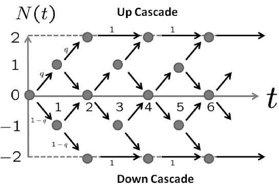
Figure 1: Simple model of information cascade. States $N(t)\in\{2,1,0,-1,-2\}$ and probabilities for $X(t)\in\{0,1\}$.

We denote the difference in the number of correct and incorrect choices up to the $t$-th individual as $N(t)$. From the above discussion, if $N(t)\geq 2(\leq-2)$, an up (down) cascade starts. There are essentially five states, $N(t)\in\{-2,-1,0,1,2\}$, if we identify all states with $N(t)\geq 2(\leq-2)$ as $N(t)=2(-2)$. If $t$ is even, there are three states, $N(t)\in\{-2,0,2\}$, and there are four states, $N(t)\in\{-2,-1,1,2\}$, if $t$ is odd. Figure 1 illustrates the model. In the figure, we also show the probabilistic rule for the transition between states. At $t=0$, $N(0)=0$, and it jumps to $N(t)=1(-1)$ with probability $q\,\,(1-q)$. From $t=1$ to $t=2$, the same rule applies, and $N(t)$ increases (decreases) by 1 with probability $q\,\,(1-q)$. If $N(t)=2(-2)$ at $t=2$, an up (down) cascade starts. Later individuals choose 1 (0) for $t\geq 3$, and $N(t)$ remains $2(-2)$. If $N(t)=0$ at $t=2$, the third individual chooses 1 with probability $q$. In general, if $|N(t)|\leq 1$, $N(t)$ increases (decreases) by 1 with probability $q\,\,(1-q)$. The problem is a random walk model with absorbing walls at $N(t)=\pm 2$. As $t$ increases, the probability that the random walk is absorbed in the walls increases. In the limit $t\to\infty$, all random walks are absorbed in the walls. The state $N(t)=0$ for even $t$ is absorbed into the state $N(t+2)=2$ with probability $q^{2}/(q^{2}+(1-q)^{2})$ and is absorbed into the state $N(t+2)=-2$ with probability $(1-q)^{2}/(q^{2}+(1-q)^{2})$. The probability for an up cascade in the limit $t\to\infty$, which we denote by $P_{2}(\infty)$, is then given as

$$P_{2}(\infty)\equiv\mbox{Pr}(N(\infty)=2)=\frac{q^{2}}{q^{2}+(1-q^{2}}.$$ (1)

In the up (down) cascade, individuals always choose 1 (0), and $P_{2}(\infty)$ is the limit value for the probability of the correct choice. It is greater than $q$ for $q>1/2$, and the deviation shows an increase in the accuracy from that of the signal. $P_{2}(\infty)-q$ is a measure of the collective intelligence.

We denote the $t$-th individual’s choice as $X(t)\in\{0,1\}$. We are interested in the estimation of the correlation function $C(t)$, which is defined as the covariance of $X(1)$ and $X(t+1)$ divided by the variance of $X(1)$. $C(t)$ can also be defined as the difference in the conditional probabilities:

$$C(t)=\mbox{Pr}(X(t+1)=1|X(1)=1)-\mbox{Pr}(X(t+1)=1|X(1)=0).$$

$C(t)$ is then estimated as

$$C(2n) = c(q)+\frac{(1-2q)^{2}}{2(q^{2}+(1-q)^{2})}(\sqrt{(2f(1-q))})^{2n},$$

$$C(2n+1) = C(2n),$$

$$c(q) = \lim_{t\to\infty}C(t)=\frac{q(1-q)}{q^{2}+(1-q)^{2}}.$$ (2)

The derivation of $C(t)$ is given in appendix A. The limit value $c(q)=\lim_{t\to\infty}C(t)$ is the order parameter of the phase transition in a nonlinear Pólya urn. The order parameter $c(q)$ changes continuously with $q$, and it takes zero at $q=0,1$. The simple model does not show a phase transition, and $C(t)$ decays exponentially with $t$.

3 Experimental Setup

The experiments reported here were conducted at Kitasato University. We performed two experiments, EXP-I and EXP-II. In EXP-I (II), we recruited $|ID|$ = 307 (33) students, mainly from the School of Science. In EXP-I (II), we prepared $I=200(33)$ questions for $q\in Q=\{5/9,6/9,7/9\}(8/15,5/9,6/9)$ and $I=400$ questions for $q=8/9$. EXP-I was performed during three periods, $q\in\{5/9,6/9\}$ in 2013, $q=7/9$ in 2014, and $q=8/9$ in 2015. EXP-II was performed in 2011. We label the questions as $i=1,2,\cdots,I$. Subjects answered $I/2\,(I)$ questions for some (all) values of $q$ in $Q$ in EXP-I (II). We obtained $I$ sequences of answers of length $T=63\,(33)$ for $q=5/9,6/9(8/15,5/9,6/9)$ in EXP-I (II). In EXP-I for $q=7/9$ and $q=8/9$, some subjects could not answer $I/2$ questions within the allotted time. The length $T$ of the sequence depends on $i$, and the average (minimum) length $T_{avg}(T_{min})$ is 54.0 (49) for $q=7/9$ and 60.5 (58) for $q=8/9$.

$|ID|$ subjects sequentially answered a two-choice question and received returns for each correct choice. We prepared $I$ questions for each $q\in Q$ by randomly choosing an urn from two different urns, urn A and urn B, which contain ball A (red) and ball B (blue) in different proportions. We denote the answer to question $q\in Q,i\in\{1,\cdots,I\}$ as $U(q,i)\in\{A,B\}$. For $q=n/m>1/2$, urn A (B) contains $n$ A (B) balls and $m-n$ B (A) balls. Urn A (B) contains more A (B) balls than B (A) balls. The subjects obtain information about urn X by knowing the color of a ball randomly drawn from it. The color of the ball is the private signal, as it is not shared with other subjects. If the ball is ball A (B), X is more likely to be A (B). Further, $q$ is the posterior probability that the randomly chosen ball suggests the correct urn and the private signal is correct. We prepared the private signal $S(q,i,t)\in\{A,B\}$ for $T$ subjects and $I$ questions in advance. In EXP-I, we controlled the ratio of the correct signal so that it was precisely $q$. Among $T$ subjects, exactly $q\cdot T$ subjects received the correct signal. In EXP-II, we did not control the private signal. Among 33 subjects, $q\cdot 33$ subjects received the correct signal on average. Table 1 summarizes the design.

Table 1: Experimental design. $|ID|$, number of subjects; $T$, length of private signal; $T_{avg}$, average length of subject sequence; $T_{min}$, minimum length of subject sequence; $\{q\}$, precision of private signal; $I$, number of questions.

Experiment	$|ID|$	$T$	$T_{avg}$	$T_{min}$	$\{q\}$	$I$
I (2013.9$\sim$ 2013.10)	126	63	63	63	$\{5/9,6/9\}$	200
I (2014.12)	109	63	54.0	49	7/9	200
I (2015.9)	121	63	60.5	58	8/9	400
II (2011.1)	33	33	33	33	$\{8/15,5/9,6/9\}$	33

Subjects answered the questions individually using their respective private signals and information about the previous subjects’ choices. This information, called social information, was given as the summary statistics of the previous subjects. If the subject answers question $q,i$ after $t-1$ subjects, the subject receives a private signal $S(q,i,t)$ and social information $\{C_{A}(q,i,t-1),C_{B}(q,i,t-1)\}$ from the previous $t-1$ subjects. Let $X(q,i,s)\in\{A,B\}$ be the $s$-th subject’s choice; the social information $C_{x}(q,i,t-1),x\in\{A,B\}$ is written as

$$C_{x}(q,i,t-1)=\sum_{s=1}^{t-1}\delta_{X(q,i,s),x},$$

where $C_{A}(q,i,t-1)+C_{B}(q,i,t-1)=t-1$ holds.

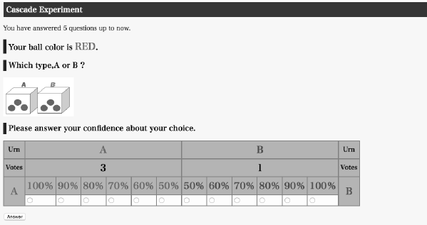
Figure 2: Snapshot of the screen for $q=6/9=2/3$ in EXP-I. The private signal is shown on the second line. The summary statistics $\{C_{A}(t),C_{B}(t)\}$ appear in the second row in the box.

Figure 2 illustrates the experience of subjects in EXP-I more concretely. The second line shows the subject’s private signal. The figure below the question shows the type of question, $q$. Before the experiment, the experimenter described the ball configuration in urns A and B and explained how the signal is related to the likelihood for each urn. The subjects can recall the question by looking at the figure. In the second row of the box, the social information is provided. In the screenshot shown in the figure, four subjects have already answered the question. Three of them have chosen urn A, and one has chosen urn B. The subject chooses urn A or urn B using the radio buttons in the last row of the box. They were asked to choose by stating how confident they are about their answer, that is, to choose 100% if they were certain about their choice and to choose 50% if they were not at all confident about their choice. The reward for the correct choice does not depend on the confidence level. Irrespective of the degree of confidence, subjects receive a positive return for the correct choice. After they chose an option and put answer button, we let them know the correct choice in the next screen. In EXP-II, the subjects were asked to choose urn A or urn B, and they were not asked to state their degree of confidence. In addition, we did not let them know the correct option. We only told them their total reward. For more details about the experimental procedure, please refer to the appendices.

Hereafter, instead of A and B, we use 1 and 0 to describe the correct and incorrect choices and private signal as in the previous section. We use the same notation for them, as follows: $S(q,i,t)\in\{0,1\}$ and $X(q,i,t)\in\{0,1\}$. For the social information, we define $\{C_{1}(q,i,t),C_{0}(q,i,t)\}$ as $C_{1}(q,i,t)\equiv C_{U(q,i)}(q,i,t)$ and $C_{0}(q,i,t)\equiv t-C_{1}(q,i,t)$. Further, $C_{1}(q,i,t)$ shows the number of correct choices up to the $t$-th subject for question $q\in Q,i\in\{1,\cdots,I\}$. In EXP-I, the length of $\{X(q,i,t)\}$ and $\{S(q,i,t)\}$ depends on $i\in I$ for $q=7/9$ and $8/9$, and one should write its dependence on $i$ explicitly as $T(q,i)$. For simplicity, we use $T$ whenever it will not cause confusion. For example, we denote the percentage up to the $t$-th subject for question $q,i$ as $Z(q,i,t)$:

$$Z(q,i,t)=\frac{1}{t}\sum_{s=1}^{t}X(q,i,s).$$

We write the final value $Z(q,i,T(q,i))$ as $Z(q,i,T)$.

4 Data Analysis

In this section, we show the results of the analysis of the experimental data. We describe how the social information and private signal affect subjects’ decisions.

4.1 Distribution of $Z(q,i,T)$

We study the relationship between the precision of the signal $q$ and $Z(q,i,T_{min})$. As we are interested in the dependence on the initial value of $X(q,i,1)$, we divide the samples according to the value of $X(q,i,1)=x$. We denote the sample number and the average value of $Z(q,i,t)$ for each case $X(q,i,1)=x$ as $I(q|x)$ and $Z_{avg}(q,t|x)$, respectively.

$$I(q|x) = \sum_{i=1}^{I}\delta_{X(q,i,1),x},$$

$$Z_{avg}(q,t|x) = \frac{\sum_{i=1}^{I}Z(q,i,t)\delta_{X(q,i,1),x}}{I(q|x)}.$$ (3)

The unconditional average value of $Z_{avg}(q,t|x)$ is then given as

$$Z_{avg}(q,t)=q\cdot Z_{avg}(q|1)+(1-q)\cdot Z_{avg}(q|1).$$

$Z_{avg}(q,t)$ corresponds to $P_{2}(t)$ in the simple model, and the deviation of $Z_{avg}(q,t)$ from $q$ is a measure of the collective intelligence.

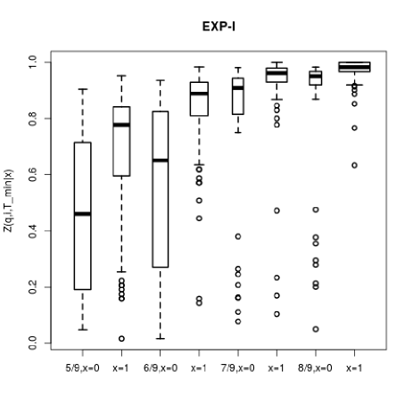
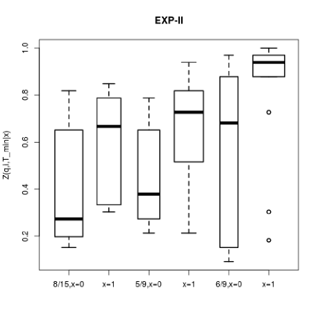
Figure 3: Boxplot of $Z(q,i,T_{min})$ in EXP-I (left) and EXP-II (right).

Figure 3 shows boxplots of $Z(q,i,T_{min})$ for the samples with $X(q,i,1)=x\in\{0,1\}$. From left to right, $q$ increases. When $q$ is small, $Z_{avg}(q,T_{min}|x)$ is small. The distribution of $Z(q,i,T_{min})$ also depends on the initial value $X(q,i,1)=x$. For $q=8/9$ in EXP-I, all $Z(q,i,T_{min})$ are larger than one-half for $x=1$. This suggests that $Z(q,i,t)$ converges to almost 1 as $t$ increases. On the other hand, if $x=0$ for $q=8/9$, there are some samples with $Z(q,i,T_{min})<1/2$. We cannot judge whether all $Z(q,i,t)$ converge to almost 1 in the limit $t\to\infty$. If $x=0$ with $q\in\{5/9,6/9\}$, the distribution of $Z(q,i,T_{min})$ is wide, suggesting the existence of multiple fixed points where $Z(q,i,t)$ converges.

Figure 4: Plot of $Z_{avg}(q,T_{min})$ and $P_{2}(\infty)$ vs. $q$. $P_{2}(\infty)$ is given by Eq. (1).

Figure 4 plots $Z_{avg}(q,T_{min})$ and $P_{2}(\infty)$ in Eq. (1) as a function of $q$. One can clearly see the collective intelligence effect, as $Z_{avg}(q,T_{min})-q$ is positive in almost all cases. For $q=8/15$ in EXP-II, the number of samples is limited and the difference is small, so there is no significant difference. One also sees that $P_{2}(\infty)$ in Eq. (1) describes $Z_{avg}(q,T_{min})$ relatively well. However, it does not mean that the experiment should be described by the simple model. As we shall see below, the system shows a phase transition, and the simple model is essentially wrong.

4.2 Strength of social influence and private signal

To measure how strongly the social information and private signal affected subjects’ decision making, we compare the correlation coefficients between them and the subjects’ decisions. We estimate the correlation coefficients as

$$\mbox{Cor}(S(t),X(t)) \equiv \frac{\overline{X(t)S(t)}-\overline{X(t)}\cdot\overline{S(t)}}{\sqrt{\mbox{V}(X(t))\mbox{V}(S(t))}},$$

$$\mbox{Cor}(Z(t-1),X(t)) \equiv \frac{\overline{X(t)Z(t-1)}-\overline{X(t)}\cdot\overline{Z(t)}}{\sqrt{\mbox{V}(X(t))\mbox{V}(Z(t))}},$$

$$\overline{A(t)} \equiv \frac{1}{I}\sum_{i=1}^{I}A(q,i,t),$$

$$\mbox{V}(A(t)) \equiv \overline{A^{2}(t)}-\overline{A(t)}^{2}.$$

Here, we also define the average value $\overline{A}$ and variance $\mbox{V}(A)$ of quantity $A$.

Figure 5: Correlation coefficients Cor$(S(t),X(t))$ and Cor$(Z(t-1),X(t))$ vs. $t$ in (a), (c) EXP-I and (b), (d) EXP-II.

Figure 5 shows plots of the correlation coefficients versus $t$. Overall, Cor$(S(t),X(t))$ decreases and Cor$(Z(t-1),X(t))$ increases with increasing $t$. In EXP-I, for $q=5/9$, Cor$(S(t),X(t))$ starts at very small values (Figure 5a). We think that subjects were confused at small $q$, and they could not trust their private signals at small $t$. However, Cor$(S(t),X(t))$ rapidly increases and behaves similarly to the other coefficients. At around $t=15$, the correlation coefficients fluctuate around certain values. The results suggest that the system becomes stationary for $t\geq 15$. Cor$(S(t),X(t))$ and Cor$(Z(t-1),X(t))$ fluctuate around 0.3 and 0.6, respectively. This indicates that the social influence is stronger than the private signal.

4.3 Response functions $f(z,s)$

We study how subjects’ decisions are affected by the social information and private signal. We study the probabilities that $X(t+1)$ takes 1 under the condition that $Z(t)=z$ and $S(t+1)=s$. We denote them as

$$f(z,s)\equiv\mbox{Pr}(X(t+1)=1|Z(t)=z,S(t+1)=s).$$

By symmetry under the transformations $S\leftrightarrow 1-S$, $X\leftrightarrow 1-X$, and $Z\leftrightarrow 1-Z$, $f(z,s)$ has the $Z_{2}$ symmetry

$$1-f(1-z,0)=f(z,1).$$

In the estimation of $f(z,s)$ using experimental data $\{S(q,i,t),X(q,i,t)\}$, we exploit the symmetry. If $S(q,i,t)=0$, we replace $(S(q,i,t)=0,Z(q,i,t-1),X(q,i,t))$ with $(1-S(q,i,t),1-Z(q,i,t-1),1-X(q,i,t))$ and estimate $f(z,1)$. Then $f(z,0)$ is given as $f(z,0)=1-f(1-z,1)$. In addition, as we are interested in the static behavior of $f(z,s)$, and Cor$(S(t),X(t))$ and Cor$(Z(t-1),X(t))$ reach their stationary values at $t=15$, we use data $\{S(q,i,t),X(q,i,t)\}$ for $t\geq 16$.

Figure 6: Response functions $f(z,1)$ for $q\in Q$ in (a) EXP-I and (b) EXP-II. $f(z,1)$ shows the probability that a subject chooses the correct urn when $z$ percent of the previous subjects chose it and the private signal is correct.

We divide the samples $\{X(q,i,t),S(q,i,t)\},16\leq t\leq T,i=1,\cdots,I$ according to the value of $Z(q,i,t-1)$. We divide them into 11 bins as $Z(q,i,t)\leq 5\%,5\%<Z(q,i,t)\leq 15\%,15\%<Z(q,i,t)\leq 25\%,\cdots,95\%<Z(q,i,t)$. We write that sample $(X(q,i,t),S(q,i,t))$ is included in bin $j\in J=\{1,2,\cdots,11\}$ as $i\in j$ and the sample number of bin $j$ as $N(q,j)=\sum_{i\in j}1$. We denote the average value of $Z(q,i,t)$ in bin $j$ as $z_{j}=\sum_{i\in j}Z(q,i,t)/N(q,j)$. After this preparation, we estimate $f(z_{j},1)$ and its error bar $\Delta f(z_{j},1)$ as

$$f(z_{j},1)=\frac{1}{N(q,j)}\sum_{i\in j}X(q,i,t)\,\,\,,\,\,\,\Delta f(z_{j},1)=\sqrt{\frac{f(z_{j},1)(1-f(z_{j},1))}{N(q,j)}}.$$

Figure 6 shows plots of $f(z_{j},1)$ versus $z_{j}$. It is clear that $f(z_{j},1)$ are monotonically increasing functions of $z_{j}$ in EXP-I. For $q=5/9,6/9$, their behaviors are almost the same. For $q=7/9,8/9$, few samples appear in the middle bins, and the error bars are large. In EXP-II, the sample numbers are smaller than those in EXP-I. We can see a strong positive dependence on $z_{j}$.

5 Detection of phase transition

In the previous section, we introduced a response function $f(z,s)$ that describes the probabilistic behavior of subjects in the experiments. For $z_{j}<z<z_{j+1},i\in\{1,\cdots,10\}$, we linearly extrapolate $f(z,s)$ with $f(z_{j},s)$ and $f(z_{j+1},s)$. For $z<z_{1}\,(>z_{11})$, we adopt $f(z,s)=f(z_{1},s)\,(f(z_{11},s))$. As the private signal takes 1 with probability $q$, the probability that the $t+1$-th subject chooses the correct option under the social influence $Z(t)=z$ is estimated as

$$f(z)\equiv\mbox{Pr}(X(t+1)=1|Z(t)=z)=q\cdot f(z,1)+(1-q)\cdot f(z,0).$$ (4)

We denote the averaged response function as $f(z)$. Then the voting process $\{X(t)\},t=1,2,\cdots$ becomes a nonlinear Pólya urn process. In this section, we study the model and verify the possibility of a phase transition.

5.1 Number of stable fixed points

Figure 7: Plot of $f(z)\equiv\mbox{Pr}(X(t+1)=1|z(t)=z)$ in EXP-I. (a) $t>15,q=5/9$ (thick solid line), 6/9 (thin solid line), 7/9 (thin broken line), and 8/9 (thick broken line). (b) $q=5/9,t>15$ (thick solid line), $q=8/9$ (thick broken line). $q\in\{5/9,8/9\},t>30$ with symbols. We plot the standard error $\Delta f(z)$ for $q=8/15$ in (a) and $t>30$ in (b).

We estimate $f(z)$ using the experimental data for EXP-I. We plot the results in Figure 7. For $q=5/9$ (thick solid line in Figure 7a), $f(z)$ crosses the diagonal at three points. The left and right fixed points are stable, and the middle one is unstable. Further, $z(t)$ converges to the two stable fixed points with positive probability, and the order parameter $c$ is positive, $c>0$. For $q=6/9$ (thin solid line in Figure 7a), $f(z)$ touches the diagonal. Considering the standard error of $f(z)$, it is difficult to judge whether it is a touchpoint. However, it strongly suggests that there is another stable fixed point or touchpoint in addition to the right stable fixed point. For $q=7/9$ (thin broken line in Figure 7a), $f(z)$ seems to have only one stable fixed point. However, the departure from the diagonal is small, and it is difficult to judge whether there is only one stable fixed point or there are two stable fixed points. For $q=8/9$ (thick broken line), there is only one stable fixed point, and $c$ is zero.

5.2 Correlation function $C(t)$

The order parameter $c$ of the phase transition is defined as the limit value of $C(t)$. $C(t)$ behaves asymptotically with three parameters, $c,c^{\prime}$ and $l>0$, as

$$C(t)\simeq c+c^{\prime}\cdot t^{l-1}.$$ (5)

If there is one stable state, $z_{+}$, $Z(t)$ converges to $z_{+}$. The memory of $X(1)=x$ in $p_{x}(t+1)$ disappears, and $c=0$. $C(t)$ decreases to zero with power-law behavior, $C(t)\propto t^{l-1}$. The exponent $l$ is given by the slope of $f(x)$ at the stable fixed point $z_{+}$ as $l=q^{\prime}(z_{+})$. If there are multiple stable states, $z_{-}<z_{+}$, the probability that $z(t)$ converges to $z_{+}$ depends on $X(1)=x$. If $c=\lim_{t\to\infty}(p_{1}(t+1)-p_{0}(t+1))$ is subtracted from $C(t)$, the remaining terms also obey a power law as $C(t)-c\propto t^{l-1}$. The exponent $l$ is given by the larger of $\{q^{\prime}(z_{+}),q^{\prime}(z_{-})\}$, as the term with the larger value governs the asymptotic behavior of $C(t)-c$ [15]. If we adopt $f(z)$ in Figure 7a, there are two stable states for $q=5/9$ and $q=6/9$. For $q=7/9$ and $q=8/9$, there is only one stable state. This suggests that a phase transition occurs depending on $q$.

We study the correlation function $C(t)$. First, $p_{x}(t+1)\equiv\mbox{Pr}(X(t+1)=1|X(1)=x)$ and their error bars $\Delta p_{x}(t+1)$ are estimated from the experimental data $\{X(q,i,t)\}$ as

$$p_{x}(t+1) = \frac{1}{N(q,x)}\sum_{i\in I}X(q,i,t+1)\delta_{X(q,i,1),x},$$

$$N_{x}(q) = \sum_{i\in I}\delta_{X(q,i,1),x},$$

$$\Delta p_{x}(t+1) = \sqrt{\frac{p(x,t+1)(1-p_{x}(t+1))}{N_{x}(q)}}.$$

$C(t)$ is then estimated as

$$C(t)=p_{1}(t+1)-p_{0}(t+1).$$

The standard error of $C(t)$ is given by

$$\Delta C(t)=\sqrt{\Delta p_{1}(t+1)^{2}+\Delta p_{0}(t+1)^{2}}.$$ (6)

Figure 8: $C(t)$ vs. $t$ in (a) EXP-I and (b) EXP-II. Error bars are estimated using Eq. (6). To see the behavior of $C(t)$ clearly, we plot only $C(t)$ for $\Delta t=5(3)$ for EXP-I (II). In addition, we shift the data for $q=5/9,6/9(8/15)$ leftward and those for $q=7/9,8/9(6/9)$ rightward for EXP-I (II).

Figure 8 shows plots of $C(t)$ for $t<T_{min}$ as a function of $t$ in EXP-I and EXP-II. In both experiments, the error bars are large. In EXP-I, $C(t)$ fluctuates around 0.25 for $q\in\{5/9,6/9\}$. For $q\in\{7/9,8/9\}$, $C(t)$ decreases and takes small values for large $t$. However, it is difficult to judge whether $C(t)$ decreases to zero or fluctuates around some positive values. In EXP-II, in all three cases, $C(t)$ seems to fluctuate around 0.2.

5.3 Estimation of $C(t)$ for $t\geq T_{min}$

As the system size $T_{min}$ in our experiments is very limited, we adopt the Pólya urn process based on Eq. (4) to simulate the system for $t>T_{min}$. We introduce a stochastic process $\{X(t)\},t\in\{1,2,3,\cdots,T\}$. $X(t+1)\in\{0,1\}$ is a Bernoulli random variable, and its probabilistic rule depends on all the previous $\{X(t^{\prime})\},t^{\prime}\in\{1,\cdots,t\}$ through $C_{1}(t)=\sum_{t^{\prime}=1}^{t}X(t^{\prime})$. The probability that $X(t+1)$ is 1 for $C_{1}(t)=n_{1}$ is given by $f(n_{1}/t)$. We denote the probability function for $\sum_{t^{\prime}=1}^{t}X(t^{\prime})=n$ with an initial condition $X(1)=x$ as $P(t,n|x)$.

$$P(t,n|x)\equiv\mbox{Pr}\left(\sum_{t^{\prime}=1}^{t}X(t^{\prime})=n|X(1)=x\right).$$

The master equation for $P(t,n|x)$ is

$$P(t+1,n|x)=f(n-1/t)\cdot P(t,n-1|x)+(1-f(n/t))\cdot P(t,n|x).$$ (7)

We use the experimental data from EXP-I as the initial condition for $t=T_{min}$ (Figure 3). We solve the master equation recursively and obtain $P(t,n|x)$ for $t\leq 10^{6}$. We estimate $C(t)$ as

$$C(t)=\sum_{n=1}^{t}P(t,n|1)\cdot f(n/t)-\sum_{n=0}^{t-1}P(t,n|0)\cdot f(n/t).$$

Figure 9 shows the plots of $C(t)$ versus $t$.

Figure 9: $C(t)$ vs. $t$ for $10^{1}\leq t<10^{6}$. For $t<T_{min}$, we plot the results in Figure 8a with $\Delta t=10$.

For $q=5/9$, $C(t)$ converges to a finite and positive value, and $c>0$. For $q=8/9$, $C(t)$ decays to zero very slowly. For $q=7/9$, $C(t)$ decays more slowly, and it takes a finite value even for $t\sim 10^{6}$. From the slope of $C(t)$ there, we can assume the limit value of $C(t)$ is zero. For $q=6/9$, the situation is more subtle. If $f(z)$ has a touch point, $C(t)$ decays logarithmically as

$$C(t)\sim c+c^{\prime}(\ln t)^{-1}.$$

In this case, it is difficult to judge whether the limit value of $C(t)$ is positive or zero, as $C(t)$ decreases too slowly. Even if it is uncertain, we can say that $c$ is positive for $q=5/9$ and zero for $q=7,9$ and $8/9$. The system shows a phase transition.

5.4 Estimation of $c$

To estimate $c$, we employ the integrated quantities of $C(t)$, which are the integrated correlation time $\tau$ and the second moment correlation time $\xi$ divided by the time horizon $t$. They are defined in terms of the moments of $C(s)$ as

$$\tau_{t}(t) \equiv \tau(t)/t=m_{0}(t)/t,$$ (8)

$$\xi_{t}(t) \equiv \xi(t)/t=\sqrt{m_{2}(t)/m_{0}(t)},$$

$$m_{n}(t) \equiv \sum_{s=0}^{t-1}C(s)(s/t)^{n}.$$ (9)

Figure 10: Plots of (a) $\tau_{t}(t)$ and (b) $\xi_{t}(t)$ vs. $t$.

By using the asymptotic behavior of $C(t)$ in Eq. (5), the limit values of $\tau_{t}(t)$ and $\xi_{t}(t)$ are found to be

$$\lim_{t\to\infty}\tau_{t}(t) = \lim_{t\to\infty}c+\frac{c^{\prime}}{l}t^{l-1}=c,$$ (10)

$$\lim_{t\to\infty}\xi_{t}(t) = \begin{cases}\sqrt{\frac{l}{l+2}}\,\,\,\,,\,\,\,\,c=0,\\ \sqrt{\frac{1}{3}}\,\,\,\,,\,\,\,\,c>0.\end{cases}$$ (11)

The limit value of $\tau_{t}(t)$ coincides with $c$. With the limit value of $\xi_{t}(t)$, we can judge whether $c>0$ or $c=0$ by $\lim_{t\to\infty}\xi_{t}(t)=\sqrt{1/3}$ or $\lim_{t\to\infty}\xi_{t}(t)<\sqrt{1/3}$.

Figure 10 shows plots of $\tau_{t}(t)$ and $\xi_{t}(t)$ versus $t$. $\tau_{t}(t)$ increases gradually with $t$ for $t>T_{min}$ and $q=5/9$. For sufficiently large $t$, $\tau_{t}(t)$ for $q=5/9$ is larger than that for $q=6/9$. For $q=7/9$ and $8/9$, $\tau_{t}(t)$ decreases to zero monotonically, suggesting that $c=0$. $\xi_{t}(t)$ for large $t$ is smaller than $3^{-1/2}$ for $q\in\{7/9,8/9\}$, also suggesting that $c=0$. For $q\in\{5/9,6/9\}$, $\xi_{t}(t)$ converges to $3^{-1/2}$ as $t$ increases, suggesting that $c>0$. From these results, we conclude that $c$ decreases with increasing $q$ for $q\in\{5/9,6/9\}$ and $c=0$ for $q\in\{7/9,8/9\}$.

5.5 Plot of $P(T,n|x=0)$

Lastly, we show the time evolution of $P(t,n|x)$ for the sample with $X(q,i,1)=x=0$. The boxplot of $Z(q,i,T_{min})$ for $x=0$ in Figure 3 shows the initial configuration for $P(T_{min},n|0)$. As there is only one stable fixed point, $z_{+}$, for $q\in\{7/9,8/9\}$, $Z(q,i,t)$ should converge to $z_{+}$. The main interest lies in whether the samples with $Z(q,i,T_{min})<1/2$ for $q\in\{7/9,8/9\}$ converge to $z_{+}$. On the other hand, for $q\in\{5/9,6/9\}$, there are two stable fixed states, and $P(t,n|0)$ should have two peaks.

Figure 11: Plots of $P(t,n|x)$ with $x=X(q,i,1)=0$ for $q\in\{5/9,6/9,7/9,8/9\}$ and $t\in\{T_{min},10^{4},10^{6}\}$.

Figure 11 shows plots of $P(t,n|0)$ for $q\in\{5/9,6/9,7/9,8/9\}$ and $t\in\{T_{min},10^{4},10^{6}\}$. $P(t,n|0)$ for $q\in\{5/9,6/9\}$ clearly has two peaks for $t=10^{6}$. However, there is also a clear difference in the convergence of $P(t,n|0)$. For $q=5/9$. the peak at the lower stable fixed point $z_{-}$ is sharp for $t=10^{6}$, suggesting that the convergence is rapid. On the other hand, for $q=6/9$, the height of the peak at the touchpoint is low, suggesting slow convergence. If $f(z)$ has a touchpoint at $q_{t}$, $Z(q,i,t)$ converges to $q_{t}$ as $|q_{t}-Z(q,i,t)|\propto(\ln t)^{-1}$ if $Z(q,i,t)$ starts below $q_{t}$. This slow convergence is reflected in the shape of the peak at $q_{t}$. For $q=8/9$, only one peak appears, and the sample with $Z(q,i,T_{min})<1/2$ converges to $z_{+}$ at $t=10^{6}$. For $q=7/9$, as the deviation of $f(z)$ from the diagonal is small, the convergence to the unique stable fixed point $q_{+}$ is remarkably slow. Even at $t=10^{6}$, a positive probability of $Z(q,i,t)<1/2$ remains. In the limit $t\to\infty$, the probability should disappear, and it is difficult to detect it experimentally.

6 Summary and Comments

We propose a new method of detecting a phase transition in a nonlinear Pólya urn in an information cascade experiment. It is based on the asymptotic behavior of the correlation function $C(t)\simeq c+c^{\prime}\cdot t^{l-1}$. The limit value $c$ of $C(t)$ is the order parameter of the phase transition. The phase transition is between the phase with $c=0$, in which there is only one stable state, and the phase with $c>0$, in which there is more than one stable state. To estimate $c$ and detect the phase transition, we propose to use the correlation times $\tau(t)$ and $\xi(t)$ divided by $t$. We perform an information cascade experiment to verify the method. The experimental setup is the canonical one in which subjects guess whether the randomly chosen urn X is urn A or urn B. We control the precision of the private signal $q$ by changing the configuration of colored balls in the urns. We successfully detected the phase transition in the system when $q$ changed. For large $q$, $c=0$, and there is only one stable state. The system is self-correcting. For small $q$, $c>0$, and there are multiple stable states. The probability that the majority’s choice is incorrect is positive.

We comment on the system size in the experiment. In this paper, we reported on two experiments, EXP-I and EXP-II, which differ mainly in the system size $T$ and sample number $I$. Regarding the system size $T$, as Cor($S(t),X(t))$ and Cor$(Z(t-1),X(t))$ fluctuate around some value for $t\geq 15$, the minimum size of $T$ should be larger than that value in order to study the stationary behavior of the system. Furthermore, to estimate $c$ from the asymptotic behavior of $C(t)$, it is necessary to estimate $f(z)$ precisely. For this purpose, $Z(q,i,t)$ should take all the values in $[0,1]$. As $t$ increases, $Z(q,i,t)$ converges to some stable fixed point of $f(z)$. We cannot gather enough data to cover all the values $z\in[0,1]$ if $t$ becomes too large. Instead of setting $T$ to be large, we should set $I$ to be large. In EXP-I, we judge that there is only one stable fixed point for $q=8/9$. The difficulty of determining phases comes from the error bars in the estimate of $f(z)$. As the error bars $\Delta f(z)$ are proportional to $1/\sqrt{I}$, $I$ should be as large as possible. to reduce $\Delta f(z)$. Considering the standard errors $\Delta f(z)$ in Figure 7, in order to judge whether there is only one stable fixed point for $f(z)$ for $q=8/9$ in EXP-I, $I$ should be four times that in EXP-I. Although $I=4\times 400=1.6\times 10^{3}$ might be large for a laboratory experiment, it is realizable in a web-based online experiment [4, 5].

Another future problem is to understand and derive the response function theoretically. A theoretical investigation using experimental data for an information cascade in a two-choice general knowledge quiz was recently performed [24]. The problem in analyzing the data for an information cascade in a general knowledge quiz is the difficulty in controlling the private signal [21]. The information cascade experiment with a two-choice urn is ideal from this viewpoint. The experimenter can control the private signal freely and study the change in the subjects’ choices. To understand the response function, it is necessary to control the number of referenced subjects. We believe that experiments along these lines should be performed. The multi-choice quiz case might be an interesting experimental subject. In that case, the corresponding nonlinear Pólya model is similar to the Potts model [25]. The problem is whether the herding strength increases or decreases as the number of options changes. We believe that the accumulation of experimental studies in these directions is important for the development of econophysics [26, 27, 28] and sociophysics [29, 30].

The authors thank Ai Sugimoto, Yusuke Kishi, Kota Kuwabata, Shunsuke Yoshida, Shion Kawasaki, and Fumiaki Sano for their support of the experiments. The authors also thank all the participants in the experiments. This work was supported by JSPS KAKENHI Grant No. 25610109.

Appendix A

We denote the probability function for $N(t)\in\{-2,-1,0,1,2\}$ with the initial condition $X(1)=x$ as

$$P_{n}(t|x)\equiv\mbox{Pr}(N(t)=n|X(1)=x).$$

$P_{0}(2n)$ is easily estimated as

$$P_{0}(2n|x)=P_{0}(2|x)\cdot(2q(1-q))^{n}.$$

$P_{\pm 2}(t)$ satisfies the following recursive relations for even $t$,

$$P_{2}(2n+2|x) = P_{2}(2n|x)+q^{2}\cdot P_{0}(2n|x),$$

$$P_{-2}(2n+2|x) = P_{-2}(2n|x)+(1-q)^{2}\cdot P_{0}(2n|x).$$ (12)

$P_{\pm 1}(t)=0$ for even $t$. For odd $t$, $P_{n}(t)$ are estimated as

$$P_{2}(2n+1|x) = P_{2}(2n|x)\,\,\,,\,\,\,P_{-2}(2n+1|x)=P_{-2}(2n|x),$$

$$P_{1}(2n+1|x) = q\cdot P_{0}(2n|x)\,\,\,,\,\,\,P_{-1}(2n+1|x)=(1-q)\cdot P_{0}(2n|x).$$ (13)

$P_{0}(t)=0$ for odd $t$. The initial condition for the recursive relation is

$$P_{0}(2|x)=q\cdot\delta_{x,0}+(1-q)\cdot\delta_{x,1},P_{2}(2|x)=q\cdot\delta_{x,1},P_{-2}(2|x)=(1-q)\delta_{x,0}.$$

By solving the recursive relations with the initial condition, we have

$$P_{2}(2n|x) = P_{2}(2|x)+q^{2}P_{0}(2|x)\cdot\frac{1-(2q(1-q))^{n-1}}{1-2q(1-q)},$$

$$P_{-2}(2n|x) = P_{-2}(2|x)+(1-q)^{2}P_{0}(2|x)\cdot\frac{1-(2q(1-q))^{n-1}}{1-2q(1-q)}.$$ (14)

The unconditional probability for an up cascade is

$$P_{2}(2n)=q\cdot P_{2}(2n|1)+(1-q)\cdot P_{2}(2n|0)=q^{2}+q^{2}\cdot 2q(1-q)\frac{1-(2q(1-q))^{n}}{1-2q(1-q)}.$$

In the limit $n\to\infty$, it converges to

$$P_{2}(\infty)\equiv\lim_{n\to\infty}P_{2}(2n)=\frac{q^{2}}{q^{2}+(1-q)^{2}}.$$

Pr$(X(2n+1)=1|X(1)=x)$ is then estimated as

$$\mbox{Pr}(X(2n+1)=1|X(1)=x)=P_{2}(2n|x)+q\cdot P_{0}(2n|x).$$

$C(2n)$ is then given as

$$C(2n)=\frac{q(1-q)}{q^{2}+(1-q)^{2}}+\frac{(1-2q)^{2}}{2(q^{2}+(1-q)^{2})}(\sqrt{(2q(1-q))})^{2n}.$$

For $t=2n+1$, we can show that $C(2n+1)=C(2n)$.

Appendix B Additional information about EXP-I

We explain EXP-I in detail. We performed the experiment in 2013, 2014, and 2015. We recruited 126, 109, and 121 subjects in 2013, 2014, and 2015, respectively.

In 2013, the duration of the experiment was 13 days; we recruited 126 subjects and performed the experiment for $q\in\{5/9,6/9\}$. Subjects had to participate in the experiment twice. In the first session, subjects answered 100 questions for $q=6/9$. After a 5 min interval, they participated in another cascade experiment. In one session, a subject had to participate in two types of information cascade experiment. In the second session, subjects answered 100 questions for $q=5/9$. After a 5 min interval, they participated in another cascade experiment. The allotted time for one session was 90 min, which included time for an explanation of the experiment. The subjects received 10 yen (about 8 cents) for each correct choice. After they participated in two sessions for two values of $q$, they were given their reward.

We performed the experiment for $q=7/9$ in 2014. The duration of the experiment was 13 days, and we recruited 109 subjects. Thirty-nine of the subjects had participated in the experiment in 2013. As in the experiment in 2013, after they answered 100 questions for $q=7/9$, they participated in another cascade experiment. A problem with the web server used for the experiment occurred on the first day in 2014, and some participants could not answer all 100 questions in the allotted time. The subjects received 5 yen (about 4 cents) for each correct choice.

In 2015, we performed the experiment for $q=8/9$. The duration of the experiment was 7 days, and we recruited 121 subjects. In the experiment, the subjects answered 200 questions for $q=8/9$ only, and they did not participate in another experiment. Ten of the subjects had participated in both of the first two experiments. Within the allowed time of about 40 min, they could not answer all questions. The subjects received 5 yen (about 4 cents) for each correct choice in addition to a payment of 150 yen (about 1.2 dollars) for participating.

Next, we explained the experimental procedure. Subjects entered a room and sat in a seat. There were two documents on the desk in front of the seat: an experimental participation consent document and a brief explanation of the experiment. The experimenter described the experiment and the reward using the document. Next, the subjects signed the consent document and logged into the experiment’s web site using IDs assigned by the experimenter. Then they started to answer the questions. After the experiment started, communication among participants was forbidden. A question was chosen by the server used for the experiment and displayed on the monitor of a 7 in. tablet (e.g., Nexus 7). There were no partitions in the room, and subjects could see each other. However, the displays on the tablets were small, and the subjects could not see which question the other subjects received and which option they chose.

Appendix C Additional information about EXP-II

We recruited 33 subjects for EXP-II. We performed the experiment in one day. Originally, we planned to obtain data for the experiment with $T=33$ and $Q=\{6/9,5/9,8/15\}$ twice within 3 h. We prepared $I=33$ questions and the private signals $U(q,i,t)$ for $T$ subjects for question $q,i$. We let all 33 subjects enter an information science laboratory, and they participated in the experiment simultaneously. Subject $j=1,\cdots,33$ answered question $i=1,\cdots,I$ as the $t=(i+j-2)\mbox{mod}33+1$-th subject. However, this procedure caused a “traffic jam,” and the server used for the experiment could not serve questions smoothly. Within the 3 h allotted, we could gather data only for the first three cases, i.e., 99 questions. Subjects received 10 yen (about 8 cents) for each correct choice. There was a payment of 3000 yen (about $25) for participating.

Appendix D Asymptotic behavior of V$(z(q,t))$

We studied the asymptotic behavior of the variance of $Z(q,t)$ and verified the possibility of the phase transition. In contrast to the method based on $C(t)$, the analysis of the variance has the advantage that it can directly detect the existence of multiple stable states. The drawback is the estimation of the standard errors, as we do not know the the distribution of $Z(q,t)$.

Figure 12: V$(Z(q,t))$ vs. $t$ in (a) EXP-I and (b) EXP-II. Solid line in (a) shows the results fitted with V$(Z,q,t)\propto t^{l-1}$ and $l=0.758$.

Figure 11 shows plots of V$(Z(q,t))$ versus $t$. For $q\in\{5/9,6/9\}$ in EXP-I and for all cases in EXP-II, V$(Z(q,t))$ seems to converge to some positive value for large $t$. The result is consistent with the result that there are multiple stable states in the system in these cases. V$(Z(q,t))$ exhibits power-law behavior as V$(Z(q,t))\propto t^{l-1}$ with $l=0.758(5)$ and $0.662(4)$ for $q=7/9$ and $q=8/9$, respectively. There is only one stable state in the system. The asymptotic behavior of V$(Z(t))$ and that of $C(t)$ is the same if $l>1/2$ [15].

Appendix E Archive of experimental data

In the arXiv site for this manuscript, we uploaded the experimental data for both experiments. The data are provided as CSV files, EXP-I.csv and EXP-II.csv. They contain $X(q,i,t),S(q,i,t),ID(q,i,t)$, and $C(q,i,t)$ for $q\in Q$, $i\in\{1,\cdots,|I|\}$, and $t\in\{1,\cdots,T\}$. Here $C(q,i,t)\in\{50\%,60\%,\cdots,100\%\}$ indicates the confidence of the subject regarding the choice $X(q,i,t)$. In EXP-II, the subject chose A or B directly instead of in terms of the confidence level, so there are no data for the confidence. $ID(q,i,t)$ are the identification numbers of the subjects. In EXP-II, $ID\in\{1,\cdots,33\}$, as there were 33 subjects. In EXP-I, in 2013, there were 126 subjects, and we labeled them as $ID\in\{1,\cdots,126\}$. In 2014, there were 109 subjects, 39 of whom had participated in the first period. We used the same IDs for these 39 subjects and labeled the remaining 70 subjects as $ID\in\{127,\cdots,196\}$. In 2015, there were 121 subjects, 10 of whom participated in both experiments in 2013 and 2014. We labeled the remaining 111 subjects as $ID\in\{197,\cdots,307\}$.

The first column in the data file is $n$ in $q=n/(n+m)$, the second column is $i$, the third column is $t$, the fourth column is $X(q,i,t)$, the fifth column is $S(q,i,t)$, the sixth column is $ID(q,i,t)$, and the last column is $C(q,i,t)$.

References

- [1] D. J. Watts: J. Consumer Research 34 (2007) 441.
- [2] D. Sumpter and S. C. Pratt: Phil. Trans. R. Soc. B364 (2009) 743.
- [3] J. Fernandez-Gracia, K. Suchecki, J. J. Ramasco, M. S. Miguel, and V. M. Eguíluz: Phys.Rev.Lett. 112 (2014) 158701.
- [4] M. J. Salganik, P. S. Dodds, and D. Watts: Science 311 (2006) 854.
- [5] R. M. Bond, C. J. Fariss, J. Jones, A. Kramer, C. Marlow, J.E.Settle, and J. Fowler: Nature 489 (2012) 295.
- [6] T. Wang and D.Wang: Big Data 2 (2014) 196.
- [7] G.Pólya: Ann. Inst. Henri Poincaré 1 (1931) 117.
- [8] M. Hisakado, K. Kitsukawa, and S. Mori: J. Phys. A 39 (2006) 15365.
- [9] R. Pemantle: Pobab. Surv. 4 (2007) 1.
- [10] W. B. Arthur: Econ. Jour. 99 (1989) 116.
- [11] B. Hill, D. Lane, and W. Sudderth: Ann. Prob. 8 (1980) 214.
- [12] M. Hisakado and S. Mori: J. Phys. A 44 (2011) 275204.
- [13] M. Hisakado and S. Mori: J. Phys. A 45 (2012) 345002.
- [14] S. Mori and M. Hisakado: J.Phys.Soc.Jpn. 84 (2015) 054001.
- [15] S. Mori and M. Hisakado: Phys.Rev. E 92 (2015) 052112.
- [16] S. Bikhchandani, D. Hirshleifer, and I. Welch: J. Polit. Econ. 100 (1992) 992.
- [17] L. R. Anderson and C. A. Holt: Am. Econ. Rev. 87 (1997) 847.
- [18] D. Kbler and G. Weizscker: Rev. Econ. Stud. 71 (2004) 425.
- [19] J. Goeree, T. R. Palfrey, B. W. Rogers, and R. D. McKelvey: Rev. Econ. Stud. 74 (2007) 733.
- [20] D. J. Watts: Proc. Natl. Acad. Sci. (USA) 99 (2002) 5766.
- [21] S. Mori, M. Hisakado, and T. Takahashi: Phys. Rev. E 86 (2012) 026109.
- [22] S. Mori, M. Hisakado, and T. Takahashi: J.Phys.Soc.Jpn. 82 (2013) 0840004.
- [23] S. Mori, M. Hino, M. Hisakado, and T. Takahashi: Proceedings of ECCS’14, arXiv:1507.07265 (2015).
- [24] V. M. Equíluz, N. Masuda, and J. Fernández-Gracia: PLoS One 10 (2015) e0121332.
- [25] M. Hisakado and S. Mori: Physica A 417 (2015) 63.
- [26] R. N. Mantegna and H. E. Stanley: Introduction to Econophysics: Correlations and Complexity in Finance (Cambridge University Press, Cambridge, 2007).
- [27] A. Kirman: Complex Economics: Individual and Collective Rationality (Routledge, 2010).
- [28] J.-P. Huang: Experimental Econophysics (Springer, 2015).
- [29] S. Galam: Int. J. Mod. Phys. C 19 (2008) 409.
- [30] C. Castellano, S. Fortunato, and V. Loreto: Rev.Mod.Phys. 81 (2009) 591.