CAUSATION ENTROPY FROM SYMBOLIC REPRESENTATIONS OF DYNAMICAL SYSTEMS

Abstract

Identification of causal structures and quantification of direct information flows in complex systems is a challenging yet important task, with practical applications in many fields. Data generated by dynamical processes or large-scale systems are often symbolized, either because of the finite resolution of the measurement apparatus, or because of the need of statistical estimation. By algorithmic application of causation entropy, we investigated the effects of symbolization on important concepts such as Markov order and causal structure of the tent map. We uncovered that these quantities depend nonmontonically and, most of all, sensitively on the choice of symbolization. Indeed, we show that Markov order and causal structure do not necessarily converge to their original analog counterparts as the resolution of the partitioning becomes finer.

While quantitative description and understanding of natural phenomena is at the core of science, inference of cause-and-effect relationships from measured data is a central problem in the study of complex systems, with many important practical applications. For example, knowing “what causes what” allows for the effective identification of the cause of a medical disease or disorder, and for the detection of the root source of defects of engineering systems. However, the act of measuring the states of a dynamical system mediates the inference of cause-and-effect relationships. For instance, all observation procedures carry the limitation of finite precision. A common example is the binning of data (histograms) into discrete symbols. In this paper we use a toy mathematical model to show that such digitization (symbolization) may lead to inferred causal relationships that differ significantly from those of the original system, even when the amount of data is unlimited. Although based on a simple mathematical model, our results shed new light on the challenging nature of causality inference.

I Introduction

Uncovering cause-and-effect relationships remains an exciting challenge in many fields of applied science. For instance, identifying the causes of a disease in order to prescribe effective treatments is of primary importance in medical diagnosis lesne ; locating the defects that could cause abrupt changes of the connectivity structure and adversely affect the performance of the system is a main objective in structural health monitoring gao ; vicente . Consequently, the problem of inferring causal relationships from observational data has attracted much attention in recent years lesne ; gao ; vicente ; schreiber2000 ; rothman05 ; palus-report ; frenzel07 ; guo08 ; heckman08 ; barrett10 ; cubitt12 ; runge12a ; runge12b ; marinazzo12 ; sun2014a ; sun2014b ; sun2014c ; porta14 .

Identifying causal relationships in large-scale complex systems turns out to be a highly nontrivial task. As a matter of fact, a reliable test of causal relationships requires the effective determination of whether the cause-and-effect is real or is due to the secondary influence of other variables in the system. This, in principle, can be achieved by testing the relative independence between the potential cause and effect conditioned on all other variables in the system. Such a method essentially demands the estimation of joint probabilities for (very) high dimensional variables from limited available data and suffers the curse of dimensionality. In practice, there are various approaches in statistics and information theory that aim at accomplishing the proper conditioning without the need of testing upon all remaining variables of the system at once palus-report ; PCbook . The basic idea behind many such approaches originates from the classical PC-algorithm PCbook , which repeatedly measures the relative independence between the cause and effect conditioned on combinations of the other variables. As an alternative, we recently developed a new entropy-based computational approach that infers the causal structure via a two-stage process, by first aggregatively discovering potential causal relationships and then progressively removing those (from the stage) that are redundant sun2014a ; sun2014b ; sun2014c .

In almost all computational approaches for inferring causal structure, it is necessary to estimate the joint probabilities underlying the given process. Large-scale data sets are commonly analyzed via discretization procedures, for instance using binning, ranking, and/or permutation methods darbellay ; bandt2002 ; amigo2005 ; staniek ; kugi ; haruna2013 . These methods generally require fine-tuning of parameters and can be sensitive to noise. On the other hand, the time-evolution of a physical system can only be measured and recorded to a finite precision, resembling an approximation of the true underlying process. This finite resolution can be characterized by means of a finite set of symbols, yielding a discretization of the phase space. Regardless of the nature and motivation of discretization, the precise impacts on the causal structure of the system is essentially unexplored. Here, we investigate the symbolic description of a dynamical system and how it affects the resulting Markov order and causal structures. Such description, based on partitioning the phase space of the system, is also commonly known as symbolization. Symbolization converts the original dynamics into a stochastic process supported on a finite sample space. Focusing on the tent map for the simplicity, clarity and completeness of computation it allows tim , we introduce numerical procedures to compute the joint probabilities of the stochastic process resulting from arbitrary partitioning of the phase space. Furthermore, we develop causation entropy, an information-theoretic measure based on conditional mutual information as a mean to determine the Markov order and (temporal) causal structure of such processes. We uncovered that a partitioning that maintains dynamic invariants of the system does not necessarily preserve its causal structure. On the other hand, both the Markov order and causal structure depend nonmonotonically and, indeed, sensitively on the partitioning.

II Phase Space Partitioning and Symbolic Dynamics

A powerful method of analyzing nonlinear dynamical systems is to study their symbolic dynamics through some topological partition of the phase space tim ; erikbook ; gora . The main idea characterizing symbolic dynamics is to represent the state of the system using symbols from a finite alphabet defined by the partition, rather than using a continuous variable of the original phase space. For more details, we refer to lind ; lind1 ; kitchens ; robinson . The issue of partitioning was shown to affect entropic computations in a nontrivial manner erik2000 ; erik2001 and, as we will highlight in the paper, is also intricate and central to a general information-theoretic description of the system.

II.1 Partition of the phase space and symbolic dynamics

Consider a discrete dynamical system given by

$$x_{t+1}=f(x_{t}),$$ (1)

where $x_{t}\in M\subset\mathbb{R}^{d}$ represents the state of the system at time $t$ and the vector field $f:M\rightarrow M$ governs the dynamic evolution of the states. A (topological) partition of the phase space $M$ is a finite collection $\mathcal{A}\overset{\text{def}}{=}\left\{A_{0}\text{,..., }A_{m}\right\}$ of disjoint open sets whose closures cover $M$, i.e.,

$$M={\displaystyle\bigcup\limits_{i=0}^{m}}\bar{A}_{i}.$$ (2)

The partition leads to the corresponding symbolic dynamics. In particular, for any trajectory $\{x_{0},x_{1},x_{2},\dots\}$ of the original dynamics contained in the union of $A_{i}$’s, the partition yields a symbol sequence $\{s_{0},s_{1},s_{2},\dots\}$ given by

$$s_{t}=\sum_{i=0}^{m}\chi_{A_{i}}(x_{t})\cdot i,$$ (3)

where $\chi_{A}$ is the indicator function defined as

$$\chi_{A}(x)=\begin{cases}1,~{}\mbox{if~{}$x\in A$},\\ 0,~{}\mbox{if~{}$x\notin A$}.\end{cases}$$ (4)

In other words, the symbolic state $s_{t}$ is determined by the open set $A_{i}$ that contains the state $x_{t}$. See Fig. 1 for a schematic illustration.

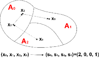
Figure 1: Schematic illustration of partitioning the phase space and the resulting symbolic dynamics. Given the partitioning $\mathcal{A}=\{A_{0},A_{1},A_{2}\}$, the trajectory $(x_{0},x_{1},x_{2},x_{3},\dots)$ leads to a symbol sequence $(s_{0},s_{1},s_{2},s_{3},\dots)=(2,0,0,1,\dots)$.

In general, the same symbol sequence may result from distinct trajectories. If the partition is generating, then every symbol sequence corresponds to a unique trajectory rudolph . A special case is the so-called Markov partition erikbook ; skufca , for which the transition from one symbolic state to another is independent of past states, analogous to a Markov process. On the other hand, a generating partition is not necessarily Markov gora ; collet .

The precise effects of partitioning on the symbolic dynamics remains an interesting and challenging problem, with recent progress in a few directions. Focusing on the equivalence between the original and symbolic dynamics, Bollt et. al. studied the consequence of misplaced partitions on dynamical invariants erik2000 ; erik2001 , while Teramoto and Komatsuzaki investigated topological change in the symbolic dynamics upon different choices of Markov partitions teramoto . On the other hand, the degree of self-sufficiency of the symbolic dynamics, irrespective of the equivalence to the original dynamics, has started to gain increasing interest, focusing on information-theoretical measures such as information closure and prediction efficiency pfante . We here adopt a different perspective and study how causal structures emerge and/or change under different choices of partitioning.

II.2 From dynamical systems to stochastic processes via symbolic dynamics

The symbolic description of a dynamical system leads naturally to an interpretation of such systems as stochastic processes gallager2013 . Let $(M,\Sigma,\mu)$ be a measure space with Borel field $\Sigma$ and probability measure $\mu$ such that $\mu:\Sigma\rightarrow[0,1]$ and $\mu(M)=1$. Furthermore, assume that $\mu$ is the unique ergodic invariant measure under the mapping $f$, that is

$$\begin{cases}\mbox{(Invariance)}~{}\mbox{For every $B\in\Sigma$, $\mu(f^{-1}(B))=\mu(B)$.}\\ \mbox{(Ergodicity)}~{}\mbox{For every $B\in\Sigma$ with $f^{-1}(B)=B$, either $\mu(B)=0$ or $\mu(B)=1$.}\end{cases}$$ (5)

Given the partitioning defined by Eq. (2), the symbol space (alphabet) $\Omega$ is made of $m+1$ symbols (alphabet letters),

$$\Omega\overset{\text{def}}{=}\{0,1,\dots,m-1,m\}.$$ (6)

We can formally define a random variable $S$ as a measurable function $S:\Omega\rightarrow\mathbb{R}$ with the probabilities given by

$$P(s_{t})\overset{\text{def}}{=}\mbox{Prob}(S_{t}=s_{t})=\mu(A_{s_{t}}),~{}\forall{s_{t}\in\Omega}.$$ (7)

This line of reasoning can be generalized to accommodate joint probabilities of arbitrary finite length,

$$P(s_{t},s_{t+1},s_{t+2},\dots) \overset{\text{def}}{=}\mbox{Prob}(S_{t}=s_{t},S_{t+1}=s_{t+1},S_{t+2}=s_{t+2},\dots)$$

$$=\mu(A_{s_{t}}\cap f^{-1}(A_{s_{t+1}})\cap f^{-2}(A_{s_{t+2}})\dots).$$ (8)

The probabilities in Eqs. (7) and (II.2) are time-invariant because $\mu$ is invariant as assumed in Eq. (5). Within this setting, $P(s)$ denotes the probability that the symbolic state of the system (at any time) is equal $s$, while $P(s,s^{\prime})$ is the probability of the current and next symbols being $s$ and $s^{\prime}$, respectively. Therefore, this framework defines a discrete stochastic process where the symbolic states are regarded as random variables whose stationary joint distributions are determined by Eqs. (7) and (II.2). We point out that the support of such a stochastic process associated with the symbolic dynamics is commonly referred to as a shift space erikbook .

III Markov Order, Causal Structure, and Inference

For a given symbolization of a dynamical system that originates from a chosen partitioning of the phase space, we are interested in defining and identifying a minimal set of past states that encode information about the current state $S_{t}$. This will enable us to remove redundant information of the past when making efficient predictions about the future.

III.1 Markov Order and Causal Structure of the Symbolic Dynamics

In view of the probabilistic interpretation of the symbol dynamics, we refer to a partition as Markovian of order $k$ if the resulting stochastic process is Markov order $k$; that is, if the symbolic state only depends on its past $k$ states rather than on the entire history. Using the following notations

$$\begin{cases}s_{t^{-}}\overset{\text{def}}{=}(s_{t-1},s_{t-2},\dots),\\ s_{t^{-}}\backslash s_{(t-k)^{-}}\overset{\text{def}}{=}(s_{t-1},s_{t-2},\dots,s_{t-k}),\end{cases}$$ (9)

a process is Markov order $k$ if and only if the conditional probabilities satisfy

$$P(s_{t}|s_{t-})=P(s_{t}|s_{t^{-}}\backslash s_{(t-k)^{-}})$$ (10)

for every choice of $s_{t^{-}}$ and no nonnegative integer smaller than $k$ fulfills this requirement. (When $k=0$, we call the process an i.i.d. process.) In other words, information carried in the past states is all conditionally redundant given information about the past $k$ states. On the other hand, there might be further redundancy in the information encoded in these $k$ states. In particular, let

$$\mathcal{P}_{t}\subset\{t-k,t-k+1,\dots,t-1\}$$ (11)

be a minimal set contained in the Markov time indices for which

$$P(s_{t}|s_{t-})=P(s_{t}|s_{\mathcal{P}_{t}})\\$$ (12)

holds for every $s_{t^{-}}$. Therefore for every proper subset $\mathcal{P}_{t}^{\prime}$ of $\mathcal{P}_{t}$ Eq. (12) does not hold. We refer to $\mathcal{P}_{t}$ as the set of causal time parents of time $t$. Conditioning on the states with time indices given by $\mathcal{P}_{t}$, information of all other states becomes redundant. The states at time(s) $\mathcal{P}_{t}$ are the only ones that cause the current state, and therefore the set $\mathcal{P}_{t}$ defines a causal structure of the symbolic dynamics. This can be viewed as a finer description than the Markov order, which in turn allows for a more efficient encoding of the process. Figure 2 illustrates the difference between Markov order and causal structure of an example process.

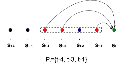
Figure 2: (Color online) An example causal structure of a Markov process. Here the process is of order $k=4$, although only three (marked in red) out of the four past time indices (enclosed by dashed box) are needed to render the current state (green) conditionally independent of the rest of the past. The set of causal time parents of $t$ is therefore $\mathcal{P}_{t}=\{t-4,t-3,t-1\}$ in Eq. (12).

III.2 Entropy, Mutual Information, Conditional Mutual Information, and Causation Entropy

Practical evaluation of joint probabilities is delicate for two reasons: first, numerical imperfections due to finite precision of the computing machines are unavoidable; second, when the probabilities need to be estimated from finite data samples, estimation errors are inevitable. Naturally, the appearance of such numerical and estimation errors will propagate into Eqs. (10) and (12), making it difficult to distinguish equalities from inequalities. These equations need to be examined for joint sequences, leading to an overwhelming number of (heuristic) decisions that need to be made. This, in turn, renders unreliable the direct determination of Markov order and causal structure based on their respective formal definitions. From a statistical standpoint, it is preferable to base such determination on a minimal number of equations/decisions. Appropriately defined information-theoretic measures fulfill this goal by collectively grouping the joint probabilities, therefore greatly reducing the number of equations/decisions.

Recall that Shannon entropy is a quantitative measure of the uncertainty of a random variable. For a discrete random variable $X$ with probability mass function $P(x)\overset{\text{def}}{=}\mbox{Prob}(X=x)$, its entropy is defined as shannon

$$H(X)=-\sum_{x}P(x)\log{P(x)},$$ (13)

where $\log$ is taken to be base $2$ throughout the paper. The mutual information between two random variables $X$ and $Y$ is given by cover

$$I(X;Y)=\sum_{x,y}P(x,y)\log\frac{P(x,y)}{P(x)P(y)}.$$ (14)

Mutual information measures the deviation from independence between $X$ and $Y$. It is generally nonnegative and equals zero if and only if $X$ and $Y$ are independent. Similarly, the conditional mutual information between $X$ and $Y$ given $Z$ is defined as cover

$$I(X;Y|Z)=\sum_{x,y,z}P(x,y,z)\log\frac{P(x,y|z)}{P(x|z)P(y|z)},$$ (15)

and it measures the reduction of uncertainty of $X$ ($Y$) due to $Y$ ($X$) given $Z$. Conditional mutual information is nonnegative, and equals zero if and only if $X$ and $Y$ are conditionally independent given $Z$.

For a stationary stochastic process $\{S_{t}\}$ and a given set of time indices $J_{t}\subset t^{-}$, we propose to define the (temporal) causation entropy (CSE) from $J_{t}$ to $t$ to be

$$C_{J_{t}\rightarrow t}=I(S_{J_{t}};S_{t}|S_{t^{-}\backslash J_{t}}).$$ (16)

Being a conditional mutual information, causation entropy is always nonnegative. It is strictly positive if and only if uncertainty about the state $S_{t}$ is reduced due to the knowledge about $S_{J_{t}}$. This occurs when the past states with time indices $J_{t}$ carry information about the current state at time $t$. We remark that Eq. (16) is an adapted definition of causation beyond our previous work sun2014a ; sun2014b ; sun2014c  for a specific scenario, in the sense that direct causality is now intimately linked to causation entropy being strictly positive without the need of appropriately choosing the conditioning set.

III.3 Inference of Markov Order and Causal Structure

Based on the definition of Markov in Eq. (10), a stochastic process has Markov order $k$ if and only if

$$C_{(t-k)^{-}\rightarrow t}=0$$ (17)

for the smallest possible nonnegative integer $k$. Algorithmically, we start by examining Eq. (17) for $k=0$. If it holds true, then the process is i.i.d. If not, we proceed with $k=1,2,\dots$, until the equation is satisfied. The resulting value of $k$ is the Markov order of the process. As a side remark, we note that there are other entropy-based approaches to determine the Markov order ragwitz2002 ; papapetrou ; pethel2014 .

Now we discuss the inference of causal structure via causation entropy. Given the definition of causal structure in Eq. (12), it follows that a Markov process of order $k$ has causal time parents $\mathcal{P}_{t}$ if and only if

$$C_{(t^{-}\backslash\mathcal{P}_{t})\rightarrow t}=0$$ (18)

where $\mathcal{P}_{t}\subset\{t-k,t-k+1,\dots,t-1\}$ and no proper subset of $\mathcal{P}_{t}$ fulfills the equation. Computationally, it is generally infeasible to efficiently find the causal structure without additional assumptions about the underlying joint distributions. A general assumption, called the faithfulness or stability assumption, requires that the joint effect/cause is decomposable into individual components  sun2014b ; PCbook ; pearl . That is to say, for every $t^{\prime}\in\mathcal{P}_{t}$, the contribution measured in terms of the conditional mutual information $I(S_{t^{\prime}};S_{t}|S_{\mathcal{Q}_{t}})$ is non-vanishing for every $\mathcal{Q}_{t}$ that does not include $t^{\prime}$ or $t$. Under this assumption, we can show that the causal time parents $\mathcal{P}_{t}$ form the minimal set of time indices that maximizes causation entropy sun2014b , i.e.,

$$\mathcal{P}_{t}=\underset{J_{t}\subset\mathcal{K}}{\bigcap}J_{t},~{}\mbox{where $\mathcal{K}=\{J\subset t^{-}:\forall K\subset t^{-},C_{J\rightarrow t}\geq C_{K\rightarrow t}\}$}.$$ (19)

We refer to Eq. (19) to as the optimal causation entropy principle, which allows the transformation of the causal inference problem into a numerical optimization problem.

Algorithmically, we propose to infer the causal set $\mathcal{P}_{t}$ via a two-stage iterative process, described as follows. The first stage, which we call aggregative discovery, starts by finding a time index $t^{\prime-}$ which maximizes the mutual information $I(S_{t^{\prime}};S_{t})$ provided that such mutual information is strictly positive. That is,

$$t_{1}=\underset{t^{\prime-}}{\operatorname{argmax}}~{}I(S_{t^{\prime}};S_{t}).$$ (20)

Then, at each subsequent step, a new time index $t_{l+1}$ is identified among the rest of the indices to maximize the conditional mutual information given the previously selected time indices, that is,

$$t_{l+1}=\underset{t^{\prime}\in\left(t^{-}\backslash\{t_{1},t_{2},\dots,t_{l}\}\right)}{\operatorname{argmax}}~{}I(S_{t^{\prime}};S_{t}|S_{t_{1},t_{2},\dots,t_{l}}).$$ (21)

Such iterative process ends when the corresponding maximum conditional mutual information equals zero, and the outcome yields a set of time indices $\mathcal{Q}_{t}=\{t_{1},t_{2},\dots,t_{L}\}\supset\mathcal{P}_{t}$.

Then, in the second stage, we progressively remove time indices in $\mathcal{Q}_{t}$ that are redundant (i.e., do not belong to $\mathcal{P}_{t}$). In particular, we enumerate through the time indices in $\mathcal{Q}_{t}$ and remove each component $t_{l}$ for which

$$I(S_{t_{l}};S_{t}|S_{\mathcal{Q}_{t}\backslash t_{l}})=0.$$ (22)

Every time a component is removed, the set $\mathcal{Q}_{t}$ is updated accordingly. The end of the process is then inferred as the set of causal time parents $\mathcal{P}_{t}$. We remark that the discovery and removal stages of our algorithm are reminiscent of the forward selection and backward elimination in regression analysis Draper . Here, for the purpose of correct and consistent inference of Markov order and causal structure, we have adopted conditional mutual information in our algorithm. sun2014b .

Two practical considerations need to be taken into account for the inference of Markov order and causal structure. First, the history of a variable needs to be truncated, i.e., $t^{-}$ will be approximated by $t^{-}\approx\{t-T,t-T+1,\dots,t-1\}$ for some $T\gg 1$ in Eq. (17) (regarding Markov order) and Eqs. (20-21) (regarding causal structure). In particular, such truncation leads to a partial fulfillment of both the Markov requirement in Eq. (10) and causal structure in Eq. (12). Second, numerical and estimation errors generally render information-theoretic quantities such as the mutual information, conditional mutual information, and causation entropy nonzero (and in particular, even negative grassberger1988 ; grassberger2008 ). In order to decide whether or not an estimate should be regarded as zero, one needs a threshold-selecting procedure sun2014b : an estimated quantity smaller than a predefined threshold will be considered vanishing.

IV Markov Order and Causal Structure from the Symbolization of Tent Map

In this section we provide an application of our theoretical procedure in determining the Markov order and causal structure of symbolic dynamics of the tent map. The primary reason why we have chosen the one-dimensional tent map as an example is twofold. First, the tent map is simple enough to allow explicit analytical computations of the entropic functionals of known probability distributions. Such computations are not only useful for cross-checking numerical estimates, they also provide some insights into the information-theoretic measures employed in our investigation. Second, regardless of its simple form, the tent map appears to serve as a rich test-bed for the investigation of how Markov order and causal structure of a dynamical system are affected by the choice of symbolization. In fact, under symbolization, even a 1D map such as the tent map can be regarded quite complex from a topological standpoint erikbook ; gora ; lind ; lind1 ; kitchens ; robinson . Finally, we remark that our computational framework can be applied to arbitrary unimodal maps.

IV.1 Tent Map and Partitioning

The tent map is a one-dimensional system given by $x_{t+1}=T(x)$ where $T:[0,1]\rightarrow[0,1]$ is defined as

$$T(x)\overset{\text{def}}{=}\begin{cases}2x,&\mbox{if~{}$0\leq x\leq\frac{1}{2}$},\\ 2(1-x),&\mbox{if~{}$\frac{1}{2}<x\leq 1$}.\end{cases}$$ (23)

Specifically, we shall discuss the manner in which different choices of the partitioning lead to (qualitatively and quantitatively) different symbolizations of the original dynamics with specific Markov orders and causal structures. For the time being, we limit our investigation to a binary symbolic description of the dynamical map. Consider a general binary partitioning of the phase space defined by the parameter $\alpha\in(0,1)$, so that

$$\mathcal{A}=\{A_{0},A_{1}\}=\{[0,\alpha),(\alpha,1]\}.$$ (24)

Such partitioning allows us to represent a continuous trajectory by a sequence of binary symbols (bits). We remark that the choice of $\alpha=0.5$ leads to a generating partition which gives rise to a symbolic dynamics that is topologically equivalent to the original system erik2000 ; erik2001 ; erikbook .

IV.2 Invariant Probability Measure and Joint Probabilities

The unique ergodic invariant measure of the tent map can be found by solving the first equation in (5) (also called a continuity equation) for each subinterval of $[0,1]$, leading to

$$\mu([a,b])=b-a.$$ (25)

This immediately gives $P(0)=\alpha$ and $P(1)=1-\alpha$. From Eq. (II.2), the joint probability of an arbitrary sequence of length $n+1$ is determined by

$$P(s_{0},s_{1},s_{2},\dots,s_{n})=\mu\left(\bigcap\limits_{l=0}^{n}I_{l}^{\left(s_{l}\right)}\right)\text{,}$$ (26)

where the intervals are defined by the preimages of $[0,\alpha)$ and $(\alpha,1]$ as

$$\begin{cases}I_{l}^{\left(0\right)}\overset{\text{def}}{=}\left\{x\in\left[0,1\right]:T^{l}\left(x\right)\in\left[0\text{, }\alpha\right)\right\},\\ I_{l}^{\left(1\right)}\overset{\text{def}}{=}\left\{x\in\left[0,1\right]:T^{l}\left(x\right)\in\left(\alpha\text{, }1\right]\right\}.\end{cases}$$ (27)

In other words, the initial conditions corresponding to a specific symbolic string of length $n$ are formed by a finite disjoint union of intervals. Figure 3 shows an example of these intervals $\{I_{l}^{(0)},I_{l}^{(1)}\}$ for $\alpha=0.45$ and four levels $l=0,1,2,3$.

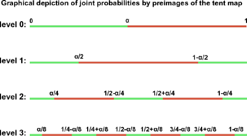
Figure 3: (Color online) Preimages of partitioning intervals of the tent map. The intervals $I_{l}^{(0)}$ (green) and $I_{l}^{(1)}$ (red) are defined by Eq. (27) and are shown for levels $l=0,1,2,3$ for the choice of $\alpha=0.45$. In general, at each level $l$, the subintervals start from $I_{l}^{(0)}$ and then alternate in between $I_{l}^{(1)}$ and $I_{l}^{(0)}$. The relative ordering of the subintervals across levels can change for different values of $\alpha$, although they remain the same as shown in the picture for all $\alpha\in(4/9,4/7)$.

This offers a computationally feasible description with which joint probabilities can be calculated. From Eq. (26), we obtain that for $n=0$, $P(s_{0})=\mu(I_{0}^{(s_{0})})$, giving $P(0)=\alpha$ and $P(1)=1-\alpha$ as expected. For $n=1$, we have $P(s_{0},s_{1})=\mu(I_{0}^{(s_{0})}\cap I_{1}^{(s_{1})})$. This gives the probabilities $P(0,0)=\alpha/2$, $P(0,1)=\alpha/2$, $P(1,0)=1-3\alpha/2$, and $P(1,1)=\alpha/2$ for all $\alpha<2/3$ (see also Fig. 3). For general values of $n$, we proceed as follows. First, we define the level-$l$ preimages of $\alpha$ to be $\{\alpha_{l}^{(i)}\}$ ($i=1,2,\dots,2^{l}$), which are the roots of the equation

$$T^{l}(x)-\alpha=0.$$ (28)

For convenience, we sort $\{\alpha_{l}^{(i)}\}$ in the ascending order of $i$ and, additionally, define $\alpha_{l}^{(0)}\overset{\text{def}}{=}0$ and $\alpha_{l}^{(2^{l}+1)}\overset{\text{def}}{=}1$. Then, the preimages sets of $[0,\alpha)$ and $(\alpha,1]$ as introduced in Eq. (27) can be explicitly computed as (for every $l\geq 1$)

$$\begin{cases}I_{l}^{(0)}=\bigcup_{i=0}^{2^{l-1}}(\alpha_{l}^{(2i)},\alpha_{l}^{(2i+1)}),\\ I_{l}^{(1)}=\bigcup_{i=1}^{2^{l-1}}(\alpha_{l}^{(2i)-1},\alpha_{l}^{(2i)}).\end{cases}$$ (29)

Such preimages sets are subsequently used to calculate joint probabilities. Note that for symbolic strings of length $n$, both the total number of joint probabilities and the total number of intervals contributing to these probabilities equal $2^{n}$.

Note that the joint probability of the symbol sequence $P(s_{0},s_{1},s_{2},\dots,s_{n})$ depends on the particular choice of the partitioning point $\alpha$. However, the functional $\alpha$-dependences of such probabilities remain the same for all $\alpha$ values within intervals determined by the $2^{n}$ distinct roots $\{x_{\ast}^{(i)}\}$ of the equation $T^{n}(x)-x=0$, given by

$$x_{\ast}^{(i)}=\begin{cases}i/(2^{n}-1),&i=0,2,\dots,2^{n}-2;\\ (i+1)/(2^{n}+1),&i=1,3,\dots,2^{n}-1.\end{cases}$$ (30)

We emphasize that although the analytical expressions derived above are specialized to the tent map, the proposed procedure is, in general, suitable for the computation of joint probabilities of arbitrary unimodal maps collet .

IV.3 Markov Order

We numerically investigate the Markov order of the stochastic processes arising from the symbolic dynamics of the tent map. Recall from Eqs. (10) and (17) that the Markov order can be determined as the smallest nonnegative integer $k$ for which the causation entropy $C_{(t-k)^{-}\rightarrow t}$ vanishes. The Markov order reveals the length of the history that carries unique information about the present symbolic state of the system.

Figure 4 shows the causation entropy $C_{(t-k)^{-}\rightarrow t}$ as a function of $k$ for a few choices of the partitioning point $\alpha$ with values equal to $0.444$, $0.47$, $0.5$, and $0.516$, respectively. For each $\alpha$, the causation entropy decreases in $k$. Such monotonic dependence of $k$ is in fact of general validity since for every $k<k^{\prime}$, the difference of causation entropies $C_{(t-k)^{-}\rightarrow t}-C_{(t-k^{\prime-}\rightarrow t}$ can be expressed in terms of a conditional mutual information, which is nonnegative. On the other hand, the mutual information $I(S_{t};S_{t-k}$, $S_{t-k+1}$,…, $S_{t-1})$ generally increases in $k$ and saturates when the causation entropy reaches zero. Results shown in Fig. 4 suggest that Markov orders can be different upon different choices of the partition point, yielding $k=3$ for $\alpha=0.444$, $k=4$ for $\alpha=0.47$, $k=0$ for $\alpha=0.5$, and $k=5$ for $\alpha=0.516$, respectively. Such difference is remarkable given the relative small differences in the values of $\alpha$.

How does the Markov order depend on the partition point $\alpha$ in general? We address this question by computing the causation entropy $C_{(t-k)^{-}\rightarrow t}$ in Eq. (17) as a function of $\alpha$ for a range of $k$ values, $k=0,1,2,\dots$. The results are shown in Fig. 5. Visually, the symbolic dynamics achieves Markov order $k$ at the values of $\alpha$ for which all curves beyond the $(k-1)$-th one reach zero. For example, Fig. 5 confirms the same Markov orders for the $\alpha$ values as shown in Fig. 4. Interestingly, the Markov order seems to depend sensitively on the choice of partitioning: a tiny bit of change in $\alpha$ generally results in a (large) change in the Markov order. This behavior is evident from the non-smooth and fractal appearance of the curves in Fig. 5 and, from the seemingly erratic manner in which they overlap and collapse.

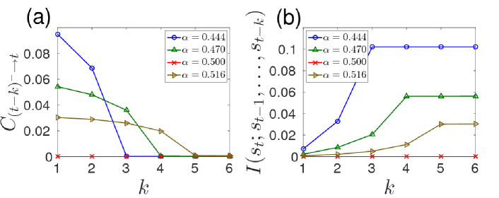
Figure 4: (Color online) Numerical determination of Markov order from causation entropy. The curves show numerically computed causation entropy $C_{(t-k)^{-}\rightarrow t}$ (a) and mutual information $I\left(S_{t};S_{t-1}\text{,..., }S_{t-k+1}\text{, }S_{t-k}\right)$(b) as functions of $k$ for various choices of $\alpha$. The results imply that the Markov order of the symbolic dynamics of the tent map equals $3$ ($\alpha=0.444$), $4$ ($\alpha=0.47$), $0$ ($\alpha=0.5$), and $5$ ($\alpha=0.516$), respectively. In the numerical calculations, we approximate $t^{-}$ by its finite truncation $(t-15,t-14,\dots,t-1)$.

Having explored the influence of the location of the partition point $\alpha$, we ask: how do partition refinements affect the Markov order? We now extend our investigation to non-binary symbolic descriptions of the tent map. Consider a map refinement of a given partitioning $\mathcal{A}=\{A_{0},A_{1},\dots,A_{m}\}$ , which is given by the intersection of the original partition elements and their preimages under $f$, as

$$\mathcal{R}(\mathcal{A})\overset{\text{def}}{=}\{f^{-1}(A_{i})\cap A_{j}\}_{i,j=0}^{m}.$$ (31)

Inspecting Eq. (II.2) and the definition of Markov order given by Eq. (10), we conclude that if the Markov order resulting from the original partition $\mathcal{A}$ is $k$, then the Markov order upon the map-refinement partition $\mathcal{R}(\mathcal{A})$ equals $k-1$ if $k>1$, and is less or equal to $1$ if $k\leq 1$ (see proof in the Appendix). This result is numerically confirmed in Fig. 6(a) for the tent map. In particular, for the original partition point $\alpha=0.5$, the Markov order equals $0$ and map refinement increases it by $1$ while further map refinement does not change the order. On the other hand, for $\alpha=0.444$ which yields Markov order $3$, each map refinement decreases its order by $1$ until the order reaches $1$. Interestingly, the same does not hold true for arbitrary refinements of the partition. Fig. 6(b) shows that a general refinement can either increase, decrease, or maintain the Markov order of the resulting process. There seems to be no predicable pattern for which the Markov order changes upon arbitrary refinement. This behavior is further explored in Fig. 6(c), which shows that for a specific initial partition (here $\alpha=0.444$), different locations of the new partition point generally result in different Markov orders. Once again, such behavior appears in an irregular pattern.

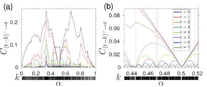
Figure 5: (Color online) Causation entropies for the symbolic states of the tent map. Causation entropies $C_{(t-k)^{-}\rightarrow t}$ (for $k=1,2,\dots,7$) are computed and shown for a range of $\alpha$ values: $\alpha\in(0,1)$(a) and $\alpha\in(0.43,0.52)$(b). Vertical dashed lines in panel (b) mark four specific choices of $\alpha$: 0.444, 0.47, 0.5, and 0.516, respectively. A grayscale bar is shown below each plotting panel to visualize the numerically determined Markov order as a function of $\alpha$, where a darker color corresponds to a higher Markov order (white corresponds to order $0$). For each $\alpha$, the Markov order is numerically determined as the smallest integer $k$ such that $C_{(t-k)^{-}\rightarrow t}<10^{-3}H(\alpha)$.

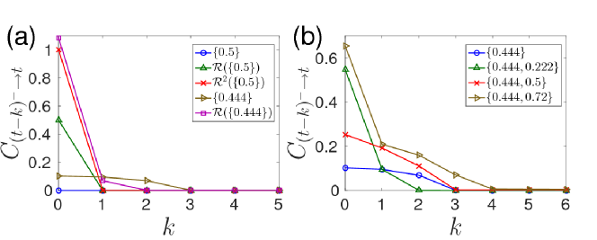
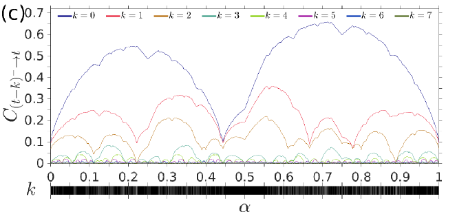
Figure 6: (Color online) Markov order upon map-refinements (a) and arbitrary refinements (b)-(c). In panels (a)-(b) the partition points are shown whereas in panel (c) the initial partition point is fixed at $0.444$ while the new partition point varies from $0$ to $1$. In all calculations, we truncated $t^{-}$ as $(t-15,t-14,\dots,t-1)$. A grayscale bar in the bottom of (c) shows the numerically computed Markov order as a function of $\alpha$, where a darker color corresponds to a higher Markov order (white corresponds to order $0$). For each $\alpha$, the corresponding Markov order is computed as the smallest integer $k$ for which $C_{(t-k)^{-}\rightarrow t}<10^{-3}H(\alpha)$.

IV.4 Causal Structure

Finally, we turn to the causal structure of a symbolic dynamics, which provides a description of the process finer than the Markov order. Unlike the Markov order, causal structure quantifies the minimal amount of the past history that is needed to mitigate the uncertainty about the present symbolic state.

For the tent map, the uncertainty of the symbolic state as measured by the entropy $H(S_{t})$ achieves its maximum at $\alpha=0.5$. Including information of past states generally reduces the uncertainty, as shown in Fig. 7(a), except at $\alpha=0.5$, which is in fact a point for which the symbolic dynamics is topologically conjugate (equivalent) to the original one. The fact that the $\alpha=0.5$ partition creates an i.i.d. process is interesting because from the dynamic equation of the system, states that are adjacent in time are intimately linked and expected to be causally related. An important conclusive message here is the following: partitioning of the phase space that results in a symbolic dynamics that is equivalent to the original dynamics can in fact yield a causal structure which differs significantly from that inferred from the form of the equations of the original system.

Recall that a process is Markov of order $k$ if no further reduction is possible beyond the $k$-th past state. However, the extent to which uncertainty is reduced does not need to be monotonic in time indices. In other words, the immediate past does not necessarily encode the most amount of information about the present state. In fact, for several values $\alpha$ (e.g., $\alpha=0.444$ and $\alpha=0.47$), the difference between conditional entropy $H(S_{t}|S_{t-k,\dots,t-1})$ for consecutive $k$’s is not monotonically decreasing in $k$ [Fig. 7(b)], vertical spacing between curves). Applying the oCSE algorithms to infer the causal structure for these $\alpha$ values, we confirmed the Markov order previously computed, and more importantly, found that the relative importance of past time states are ordered in a non-monotonic manner, namely $(t-2,t-3,t-1)$ for $\alpha=0.444$ (Markov order $k=3$) and $(t-3,t-2,t-1,t-4)$ for $\alpha=0.47$ (Markov order $k=4$). We examine all values of $\alpha$ in the interval $[0,1]$ in a uniform manner: $\{0,0.001,0.002,\dots,0.999,1\}$, using a threshold value of $10^{-3}H(\alpha)$ for the causation entropy at the given $\alpha$. The results are shown in Fig. 8. In particular, we found several examples for which the Markov order satisfies $k\leq 6$ while the number of causal parents is strictly less than $k$ (i.e., certain Markov time indices are skipped in the causal structure).

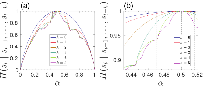
Figure 7: (Color online) Uncertainty quantification of symbolic states of the tent map. (Conditional) entropies $H\left(S_{t}\left|S_{t-1}\text{,..., }S_{t-k+1}\text{, }S_{t-k}\right.\right)$ for values of $k=0,1,\dots,5$, for the entire range of $\alpha\in(0,1)$(a) and a subrange $\alpha\in(0.43,0.52)$(b). Vertical dashed lines in both panels mark four specific choices of $\alpha$: 0.444, 0.47, 0.5, and 0.516, respectively.

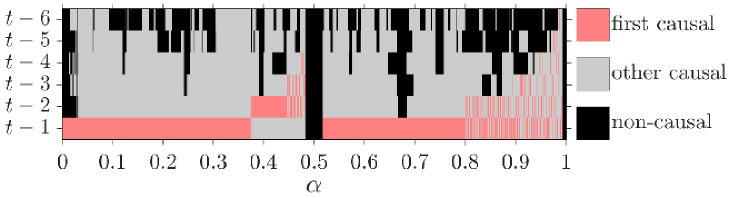
Figure 8: (Color online) Causal structures from the symbolic dynamics of the tent map when the partition point $\alpha$ is chosen from $0,0.001,0.002,\dots,0.999,1$. For each $\alpha$ we distinguish the first causal parent computed from the forward (aggregative discovery) step of the oCSE algorithm (light red), all causal parents of $t$ from the set $\{t-1,t-2,\dots,t-6\}$ (gray), and noncausal components (black). In all computations we used a threshold $10^{-3}H(\alpha)$ under which causation entropy is regarded as zero.

V Summary and Final Remarks

Symbolization is a common practice in data analysis: in the field of dynamical systems, it bridges topological dynamics and stochastic processes through partitioning/symbolization of the phase space; in causality inference, it allows for the description of continuous random variables by discrete ones. Symbolized data, in turn, are not as demanding in terms of precision and are often considered more robust with respect to parameters and noise staniek ; kugi ; crutchfield .

Motivated by the problem of uncovering causal structures from finite, discrete data, we investigated the symbolization of outputs from a simple dynamical system, namely the tent map. We provided a full description of the joint probabilities occurring from partitioning/symbolization of the phase space and investigated how Markov order and causal structure can be determined from these probabilities in terms of causation entropy, an information-theoretical measure. We found that in general, partitioning of the phase space strongly influences the Markov order and causal structure of the resulting stochastic process in an irregular manner which is difficult to classify and predict. In particular, a small change in the partition can lead to relatively large and unexpected changes in the resulting Markov order and causal structure. To the best of our knowledge, this is the first attempt in the literature that aims at unravelling the intricate dependence of inferred causal structures of dynamical systems on their different symbolic descriptions analyzed in an information-theoretic setting. Furthermore, although the effects of map refinements are well understood, it remains a main challenge to discover the exact consequences of arbitrary refinements. Especially for this reason, we have left the application of our approach to more complex dynamical systems and/or experimental time-series data to future investigations.

On a different perspective, we note that although finding partitions that preserve dynamical invariants (i.e., generating partitions) are known to be a real challenge especially for high-dimensional systems grass1985 ; lai1999 ; davidchack2000 , it is yet unclear whether or not such challenge remains when considering partitions that maintain Markov order and/or causal structure. This venue of research can be especially interesting to explore given recent advances in many different perspectives on partitioning the phase space including adaptive binning darbellay , ranking and permutation of variables bandt2002 ; amigo2005 ; staniek ; kugi ; haruna2013 ; pompe2011 , and nearest-neighbor statistics frenzel07 ; kraskov04 ; vejmelka08 ; vlachos10 ; porta2013 .

Finally, we remark that the non-uniqueness of symbolic descriptions of a system implies that important concepts such as the Markov order and causal structure are not necessarily absolute concepts: rather, they unavoidably depend on the observational process, just like classical relativity of motion and quantum entanglement cafaro12 . This, in turn, suggests the possibility of the causal structure of the very same system to be perceived differently, even given unlimited amount of data. The concept of causality, therefore, is observer-dependent.

Appendix A Monotonic Dependence of Markov Order on Map Refinements

We will prove that for a transformation $f$ that has a uniquely ergodic invariant probability measure $\mu$, the Markov order of the stochastic process resulting from a partition $\mathcal{A}$ of the phase space decreases strictly by one under a map refinement of the partition unless the original Markov order is less or equal to one.

Definition: Markov order of a partition. Consider a measure-preserving transformation $f:M\rightarrow M$ on a compact metric space with a uniquely ergodic invariant probability measure $\mu$ KatokBook . Let $\mathcal{A}=\{A_{i}\}_{i=0}^{m}$ be a measurable partition of the phase space that yields a stochastic process with time-invariant joint probabilities

$$P(s_{t}=i_{t},s_{t-1}=i_{t-1},\dots,s_{t-\ell}=i_{t-\ell})\overset{\text{def}}{=}\mu\left(A_{i_{t-\ell}}\cap f^{-1}(A_{i_{t-\ell+1}})\dots\cap f^{-\ell}(A_{i_{t}})\right).$$ (32)

If such a process is Markov of order $k$, we define the Markov order of the partition to be $k$.

Remark: In the definition, the uniqueness of the invariant measure implies ergodicity and ensures the well-definiteness of the joint probabilities KatokBook .

Definition: map refinement. Consider a measure-preserving transformation $f:M\rightarrow M$ with a probability measure $\mu$. The map refinement of a given measurable partition $\mathcal{A}=\{A_{i}\}_{i=0}^{m}$ is defined as the partition

$$\mathcal{R}(\mathcal{A})\overset{\text{def}}{=}f^{-1}(\mathcal{A})\vee\mathcal{A}=\{f^{-1}(A_{i})\cap A_{j}\}_{i,j=0}^{m}.$$ (33)

Theorem (Markov order upon map refinement.) Consider a measure-preserving transformation $f:M\rightarrow M$ on a compact metric space with a uniquely ergodic invariant probability measure $\mu$. Let $\mathcal{A}=\{A_{i}\}_{i=0}^{m}$ be a partition of $M$ and $\mathcal{R}(\mathcal{A})$ be its map refinement. Suppose that the Markov order of $\mathcal{A}$ and $\mathcal{R}(\mathcal{A})$ are $k$ and $\tilde{k}$, respectively. It follows that $\tilde{k}\leq 1$ for $k\leq 1$, and $\tilde{k}=k-1$ when $k>1$.
Proof. We shall denote the probabilities resulting from the map refinement of $\mathcal{A}$ as

$$\tilde{P}\left(\tilde{s}_{t}=(i_{t},j_{t}),\tilde{s}_{t-1}=(i_{t-1},j_{t-1}),\dots,\tilde{s}_{t-\ell}=(i_{t-\ell},j_{t-\ell})\right)$$

$$\overset{\text{def}}{=}\mu\left(\tilde{A}_{i_{t-\ell},j_{t-\ell}}\cap f^{-1}(\tilde{A}_{i_{t-\ell+1},j_{t-\ell+1}})\dots\cap f^{-\ell}(\tilde{A}_{i_{t},j_{t}})\right),$$ (34)

where $\tilde{A}_{i,j}\overset{\text{def}}{=}f^{-1}(A_{i})\cap A_{j}$. Since every sequence $\{\tilde{s}_{t}\}$ is determined by some orbit $\{x_{t}\}$ of $f$ under the partition $\mathcal{R}(\mathcal{A})$, it follows that $\tilde{s}_{t}=(i_{t},j_{t})$ if and only if $x_{t}\in f^{-1}(A_{i_{t}})\cap A_{j_{t}}$. On the other hand, $x_{t}=f(x_{t-1})$ implies that $x_{t}\in A_{i_{t-1}}$. Therefore $j_{t}=i_{t-1}$ in Eq. (A) and

$$\tilde{P}\left(\tilde{s}_{t}=(i_{t},j_{t}),\tilde{s}_{t-1}=(i_{t-1},j_{t-1}),\dots,\tilde{s}_{t-\ell+1}=(i_{t-\ell+1},j_{t-\ell+1})\right)$$

$$=P(s_{t}=i_{t},s_{t-1}=i_{t-1},\dots,s_{t-\ell}=i_{t-\ell})$$ (35)

for all sequences $(i_{t},i_{t-1},\dots)$ with nonvanishing probability. Then, the Theorem follows from applying Eq. (A) to the definition of Markov order given in Eq. (10) rewritten using the product rule (chain rule) of conditional probability. $\blacksquare$

References

- (1) A. Lesne, Chaos in biology, Rivista di Biologia-Biology Forum 99, 413-428 (2006).
- (2) Q. Gao, X. Duan, and H. Chen, Evaluation of effective connectivity of motor areas during motor imagery and execution using conditional Granger causality, NeuroImage 54, 1280 (2011).
- (3) R. Vicente, M. Wibral, M. Lindner, and G. Pipa, Transfer entropy-a model-free measure of effective connectivity for the neurosciences, J. Comput. Neurosci. 30, 45 (2011).
- (4) T. Schreiber, Measuring information transfer, Phys. Rev. Lett. 85, 461 (2000).
- (5) K. J. Rothman and S. Greenland, Causation and causal inference in epidemiology, Am. J. Public Health 95, S144 (2005).
- (6) K. Hlavackova-Schindler, M. Palus, M. Vejmelka, and J. Bhattacharya, Causality detection based on information-theoretic approaches in time series analysis, Phys. Rep. 441, 1 (2007).
- (7) S. Frenzel, and B. Pompe, Partial mutual information for coupling analysis of multivariate time series, Phys. Rev. Lett. 99, 204101 (2007).
- (8) S. Guo, A. K, Seth, K. M. Kendrick, C. Zhou, and J. Feng, Partial Granger causality—Eliminating exogenous inputs and latent variables, J. Neurosci. Methods 172, 79 (2008).
- (9) J. J. Heckman, Econometric causality, Int. Stat. Rev. 76, 1 (2008).
- (10) A. B. Barrett, L. Barnett, and A. K. Seth, Multivariate granger causality and generalized variance, Phys. Rev. E 81, 041907 (2010).
- (11) T. S. Cubitt, J. Eisert, and M. W. Wolf, Extracting dynamical equations from experimental data is NP hard, Phys. Rev. Lett. 108, 120503 (2012).
- (12) J. Runge, J. Heitzig, V. Petoukhov, and J. Kurths, Escaping the curse of dimensionality in estimating multivariate transfer entropy, Phys. Rev. Lett. 108, 258701 (2012).
- (13) J. Runge, J. Heitzig, N. Marwan, and J. Kurths, Quantifying causal coupling strength: A lag-specific measure for multivariate time series related to transfer entropy, Phys. Rev. E 86, 061121 (2012).
- (14) D. Marinazzo, M. Pellicoro, and S. Stramaglia, Causal information approach to partial conditioning in multivariate data sets, Comput. Math. Methods Med. 2012, 303601 (2012).
- (15) J. Sun and E. M. Bollt, Causation entropy identifies indirect influences, dominance of neighbors and anticipatory couplings, Physica D 267, 49 (2014).
- (16) J. Sun, D. Taylor, and E. M. Bollt, Causal network inference by optimal causation entropy SIAM Journal on Applied Dynamical Systems 14, 73–106 (2015).
- (17) J. Sun, C. Cafaro, and E. M. Bollt, Identifying coupling structure in complex systems through the optimal causation entropy principle, Entropy 16, 3416 (2014).
- (18) A. Porta, L. Faes, V. Bari, A. Marchi, T. Bassani et. al., Effect of Age on Complexity and Causality of the Cardiovascular Control: Comparison between Model-Based and Model-Free Approaches, PLoS One 9 e89463 (2014).
- (19) P. Spirtes, C. N. Glymour, and R. Scheines, Causation, Prediction, and Search, MIT Press (2000).
- (20) G. A. Darbellay and I. Vajda, Estimation of the information by an adaptive partitioning of the observation space, IEEE Transactions on Information Theory 45, 1315 (1999).
- (21) C. Bandt and B. Pompe, Permutation entropy: a natural complexity measure for time series, Phys. Rev. Lett. 88, 174102 (2002).
- (22) J. M. Amigo, M. B. Kennel, and L. Kocarev, The permutation entropy rate equals the metric entropy rate for ergodic information sources and ergodic dynamical systems, Physica D210, 77 (2005).
- (23) M. Staniek and K. Lehnertz, Symbolic transfer entropy, Phys. Rev. Lett. 100, 158101 (2008).
- (24) D. Kugiumtzis, Transfer entropy on rank vectors, Journal of Nonlinear Systems and Applications 3, 73 (2012).
- (25) T. Haruna and K. Nakajima, Symbolic transfer entropy rate is equal to transfer entropy rate for bivariate finite-alphabet stationary ergodic Markov processes, The European Physical Journal B 86, 1 (2013).
- (26) K. T. Alligood, T. D. Sauer, and J. A. Yorke, Chaos: An Introduction to Dynamical Systems, Springer-Verlag New York, Inc. (1996).
- (27) E. M. Bollt and N. Santitissadeekorn, Applied and Computational Measurable Dynamics, Society for Industrial and Applied Mathematics (2013).
- (28) A. Boyarsky and P. Gora, Laws of Chaos: Invariant Measures and Dynamical Systems in one Dimension. Probability and Its Applications, Birkhauser Boston, Boston, MA (1997).
- (29) D. A. Lind and B. Marcus, An Introduction to Symbolic Dynamics and Coding, Cambridge University Press, Cambridge, UK (1995).
- (30) D. Lind, Multi-dimensional symbolic dynamics, Proc. Symp. Appl. Math. 60, 61 (2004).
- (31) B. Kitchens, Symbolic Dynamics: One-Sided, Two-Sided, and Countable State Markov Shifts, Springer (1998).
- (32) E. A. Robinson, Jr., Symbolic dynamics and tiling in , Proc. Symp. Appl. Math. 60, 81 (2004).
- (33) E. M. Bollt, T. Stanford, Y.-C. Lai, and K. Zyczkowski, Validity of threshold-crossing analysis of symbolic dynamics from chaotic time series, Phys. Rev. Lett. 85, 3524 (2000).
- (34) E. M. Bollt, T. Stanford, Y.-C. Lai, and K. Zyczkowski, What symbolic dynamics do we get with a misplaced partition? On the validity of threshold crossing analysis of chaotic time-series, Physica D154, 259 (2001).
- (35) D. J. Rudolph, Fundamentals of Measurable Dynamics, Ergodic Theory and Lebesgue Spaces, Clarendon Press, Oxford (1990).
- (36) E. M. Bollt and J. Skufca, Markov Partitions, Encyclopedia of Nonlinear Science. Editor: A. Scot, Routledge, New York, 2005.
- (37) P. Collet and J.-P. Eckmann, Iterated maps on the interval as dynamical systems, Birkhauser Boston (2009).
- (38) H. Teramoto and T. Komatsuzaki, How does a choice of Markov partition affect the resultant symbolic dynamics? Chaos 20, 037113 (2010).
- (39) O. Pfante, E. Olbrich, N. Bertschinger, N. Ay, and J. Jost, Closure measures for coarse-graining of the tent map, Chaos 24, 013136 (2014).
- (40) R.G. Gallager, Stochastic Processes, Theory for Applications, Cambridge University Press, Cambridge, UK (2013).
- (41) C. E. Shannon, A mathematical theory of communication, Bell System Technical Journal 27, 379 (1948).
- (42) T. M. Cover and J. A. Thomas, Elements of Information Theory, 2nd Edition. John Wiley Son, Inc., Hoboken, New Jersey, USA, 2006.
- (43) M. Ragwitz and H. Kantz, Markov models from data by simple nonlinear time series predictors in delay embedding spaces, Phys. Rev. E 65, 056201 (2002).
- (44) M. Papapetrou and D. Kugiumtzis, Markov chain order estimation with conditional mutual information, Physica A 392, 1593 (2013).
- (45) S. D. Pethel and D. W. Hahs, Exact significance test for Markov order, Physica D 269, 42 (2014).
- (46) J. Pearl, Causality: Models, Reasoning, and Inference, 2nd Edition. Cambridge University Press, Cambridge, UK, 2009.
- (47) N. Draper and H. Smith, Applied Regression Analysis, 2nd Edition, John Wiley Sons, Inc., New York, 1981.
- (48) P. Grassberger, Finite sample corrections to entropy and dimension estimates, Phys. Lett. A 128, 369 (1988).
- (49) P. Grassberger, Entropy estimates from insufficient samplings, arXiv:physics/0307138 (2008).
- (50) J. P. Crutchfield and N. H. Packard, Symbolic dynamics of one-dimensional maps: entropies, finite precision, and noise, Int. J. Theor. Phys. 21, 433 (1982).
- (51) P. Grassberger and H. Kantz, Generating partitions for the dissipative Henon map, Phys. Lett. A113, 235 (1985).
- (52) Y.-C. Lai, E. M. Bollt, and C. Grebogi, Communicating with chaos using two-dimensional symbolic dynamics, Phys. Lett. A255, 75 (1999).
- (53) R. L. Davidchack, Y.-C. Lai, E. M. Bollt, and M. Dhamala, Estimating generating partitions of chaotic systems by unstable periodic orbits, Phys. Rev. E 61, 1353 (2000).
- (54) B. Pompe and J. Runge, Momentary information transfer as a coupling measure of time series, Phys. Rev. E 83, 051122 (2011).
- (55) A. Kraskov, H. Stogbauer, and P. Grassberger, Estimating mutual information, Phys. Rev. E 69, 066138 (2004).
- (56) M. Vejmelka and M. Palus, Inferring the directionality of coupling with conditional mutual information, Phys. Rev. E 77, 026214 (2008).
- (57) I. Vlachos and D. Kugiumtzis, Nonuniform state-space reconstruction and coupling detection, Phys. Rev. E 82 016207 (2010).
- (58) A. Porta, P. Castiglioni, V. Bari, T. Bassani, A. Marchi, A. Cividjian, L. Quintin, and M. Di Rienzo, -nearest-neighbor conditional entropy approach for the assessment of the short-term complexity of cardiovascular control, Physiol. Meas. 34, 17 (2013).
- (59) C. Cafaro, S. Capozziello, and S. Mancini, On relativistic quantum information properties of entangled wave vectors of massive fermions, Int. J. Theor. Phys. 51, 2313 (2012).
- (60) A. Katok and B. Hasselblatt, Introduction to the Modern Theory of Dynamical Systems, Cambridge University Press (1995).