Reduced-Set Kernel Principal Components Analysis for Improving the Training and Execution Speed of Kernel Machines

Abstract

This paper presents a practical, and theoretically well-founded, approach to improve the speed of kernel manifold learning algorithms relying on spectral decomposition. Utilizing recent insights in kernel smoothing and learning with integral operators, we propose Reduced Set KPCA (RSKPCA), which also suggests an easy-to-implement method to remove or replace samples with minimal effect on the empirical operator. A simple data point selection procedure is given to generate a substitute density for the data, with accuracy that is governed by a user-tunable parameter $\ell$. The effect of the approximation on the quality of the KPCA solution, in terms of spectral and operator errors, can be shown directly in terms of the density estimate error and as a function of the parameter $\ell$. We show in experiments that RSKPCA can improve both training and evaluation time of KPCA by up to an order of magnitude, and compares favorably to the widely-used Nyström and density-weighted Nyström methods.

1 Introduction

Modern problems in machine learning are characterized by large, often redundant, high-dimensional datasets. To interpret and more effectively use high-dimensional data, a simplifying assumption often made is that the data lies on an embedded manifold. Recovery of the underlying manifold aids certain machine learning problems such as deriving a classifier from the data, or estimating a function of interest. Algorithms that try to recover this underlying structure within the field of manifold learning include methods such as Laplacian eigenmaps [3] and diffusion maps [6]. Many such methods can be thought of as Kernel PCA (KPCA) [12] performed on specially constructed kernel matrices [9]. We denote this class of methods as Kernel Manifold Learning Algorithms. For a dataset with $n$ points, KMLAs involve the eigendecomposition of an $n\times n$ kernel matrix $K$, and a manifold mapping of order $\mathcal{O}(n)$ in cost (for a dataset with $n$ points), which limits their usefulness in some application domains (e.g., online learning and visual tracking). In addition to the computational cost, storage of the kernel matrix in memory becomes difficult for larger datasets, particularly for kernels such as the Gaussian which tends to generate dense matrices. Therefore a truly scalable KMLA method should be one that 1) avoids the computation of the full kernel matrix, 2) has low training cost, and 3) has low testing cost.

Existing methods for speeding up the computation time of KMLAs focus on the training and testing phases separately. Examples of the former include methods such as Incomplete Cholesky Decomposition (ICD) [13], the Nyström method [7] and random projections[1], which compute a low rank approximation of the kernel matrix in terms of the original dataset with $n$ points and a subset of $m$ points (see [20] and the references therein). While exhibiting excellent performance, ICD, random projections and certain Nyström methods require the computation of the kernel matrix. An example of a Nyström method that does not require the computation of a kernel matrix is one where the centers are chosen uniformly from the data. While performing well in practice, it suffers from the lack of a principled way to choose the number of centers. Related work in the class is [20], which employs $k$-means clustering and a density-weighted Gram matrix for performing KPCA. Drawbacks to the approach include the use of $k$-means, which also requires the number of clusters in advance and can be slow in high dimensions (due to its iterative nature); and an asymmetric weighted Gram matrix. Further, both methods require the retention of the full dataset for computing projections; while the training cost may be lower, the testing cost remains the same.

Methods to reduce the testing cost include reduced set selection and sparse selection methods, which find a reduced set of expansion vectors from the original space that approximate well the training set [11, 15], reduced set construction, which identifies new elements of the input space that approximate well the training set [11], and kernel map compression, which uses generalized radial basis function networks to approximate the kernel map [2]. Given that the full eigendecomposition is typically required, these methods tend to be expensive in training, but can reduce the testing cost significantly.

Approach. To the authors’ knowledge, no method exists which considers speeding up both training and testing of KMLAs in a unified and principled manner. This paper proposes to do so by connecting kernel principal component analysis to the eigendecomposition of kernel smoothing operators. In particular, given a sampled data set $\{x_{i}\}_{1}^{n}$, we show that the spectral decomposition of the Gram matrix $K$ is related to the kernel density estimate $\widehat{p}(x)$. If an approximation $\widetilde{p}(x)$ is available whose cardinality is much lower than that of $\widehat{p}(x)$, an approximation to the original Gram matrix can be computed at a significantly reduced computational cost, thus improving the execution of KMLAs.

Contribution. There are two main contributions in the paper. This paper first exploits the connection of kernel smoothing to the spectral decomposition of integral operators, within the context of kernel principal component analysis (KPCA), to define reduced set KPCA (RSKCPA). RSKPCA relies on the existence of a reduced set density estimate (RSDE) of the dataset, with a cardinality of $m$ rather than $n$ (where $m\ll n$). The RSDE defines a weighted $m\times m$ Gram matrix $\widetilde{K}$, whose eigendecomposition is computed in lieu of the empirical Gram matrix $K$. The RSKPCA approach circumvents the computation of the full kernel matrix so that the eigendecomposition is of order $\mathcal{O}({m}^{3})$ cost instead of $\mathcal{O}({n}^{3})$. Evaluation time is also reduced, as mapping a test point into the reduced eigenspace requires $O(km)$ operations rather than $O(kn)$, with $k$ retained eigenvectors.

While many methods can be used to generate the reduced set approximation $\widetilde{p}(x)$ to the empirical density $\widehat{p}(x)$, efficient methods are preferred in order to truly impact the overall training time. This paper proposes a simple, fast, single-pass method relying on the concept of the ‘shadow’ of a radially-symmetric kernel to generate the approximation $\widetilde{p}(x)$, called the shadow density estimate (ShDE). The ShDE depends on a user-tuned parameter $\ell$ to arrive at an RSDE of cardinality $m\ll n$ with a run-time cost of $\mathcal{O}({mn})$. Unlike previous work where $m$ is chosen arbitrarily, $\ell$ is related to the kernel, and can generally be set to a generic value (say $\ell=4$) for a wide variety of problems.

The shadow algorithm enables the derivation of closed form error bounds of the RSDE and RSKPCA results. Results bounding (1) the approximation of the density via the Maximum Mean Discrepancy (MMD), (2) the eigenvalue difference between the operators $K$ and $\widetilde{K}$, and (3) the difference in Hilbert-Schmidt norm between the operators and their eigenspace projections, provide further theoretical justification for the approach. The bounds are given in terms of the user-tuned parameter $\ell$. The latter two bounds are shown to be directly related to the first bound, indicating the importance of the density estimate in generating a correct eigendecomposition. The proposed approach performs well as a substitute for the Nyström family of algorithms. While the application of choice in this paper is KMLAs, the method is applicable any problem which satisfies the assumptions and which can be formulated as a kernel eigenvalue problem.

Organization. Section 2 reviews the operator view of KPCA. Theoretical support for reduced set KPCA (RSKPCA) follows in Section 3, which uses the connection to kernel smoothing to define RSKPCA. Section 4 defines the shadow of the kernel from which the shadow density estimate (ShDE) is derived and used in the RSKPCA algorithm. Section 5 provides error bounds on the MMD distance between the KDE and the ShDE, and the approximation of the operator by RSKPCA. Section 6 reports experimental results, which show the efficacy of the method on speeding up KPCA and KPCA-based methods.

2 KPCA and Eigenfunction Learning

This section briefly summarizes the foundations of KPCA as regards the spectral decomposition of operators. To start, let $k:\mathbb{R}^{d}\times\mathbb{R}^{d}\to\mathbb{R}$ be a bounded, positive-definite kernel function, defined on the domain $D\subset\mathbb{R}^{d}$. Then $k$ has the property $k(x,y)=\langle\psi(x),\psi(y)\rangle_{\mathcal{H}}$ where $\mathcal{H}$ is a Reproducing Kernel Hilbert space and $\psi:\mathbb{R}^{d}\to\mathcal{H}$ is an implicit mapping. The kernel induces a linear operator ${\mathbf{K}}:\mathcal{L}^{2}(D)\to\mathcal{L}^{2}(D)$,

$$({\mathbf{K}}f)(x):=\int_{D}k(x,y)f(y)dy.$$ (1)

To incorporate data arising from a probability density ${p}(x)$, (1) can be modified. Let $\mu$ be a probability measure on $D$ associated to ${p}$, and denote by $\mathcal{L}^{2}(D,\mu)$ the space of square integrable functions with norm $\|f\|_{p}^{2}=\langle f,f\rangle_{p}=\int_{D}f(x)^{2}d\mu(x)$. Define the linear operator $\widetilde{\mathbf{K}}:\mathcal{L}^{2}(D,\mu)\to\mathcal{L}^{2}(D,\mu)$ by

$$(\widetilde{\mathbf{K}}f)(x):=\int_{D}k(x,y)f(y){p}(y)dy.$$ (2)

The operator $\widetilde{\mathbf{K}}$ is associated to the eigenproblem

$$\int_{D}k(x,y){p}(x)\phi_{\iota}(x)dx=\lambda_{\iota}\phi_{\iota}(y),$$ (3)

where $\phi_{\iota}(\cdot)$ are the eigenfunctions. In practice, given a sample set $\mathcal{X}=\{x_{i}\}_{1}^{n}$ drawn from ${p}(x)$, the empirical approximation to (3) is derived from the approximation

$$\int_{D}k(x,y){p}(x)\phi_{\iota}(x)dx\approx\frac{1}{n}\sum_{i=1}^{n}k(x_{i},y)\phi_{\iota}(x_{i}),$$ (4)

as obtained from the empirical estimate of the probability density ${p}(x)$ using $\mathcal{X}$,

$${p}(x)\approx\frac{1}{n}\sum_{i=1}^{n}\delta(x_{i},x),$$ (5)

which employs the sampling property of the delta function. Equation (4) then leads to the eigendecomposition of the Gram matrix $K$

$$K\hat{\phi}_{i}=\hat{\lambda}_{i}\hat{\phi}_{i},\quad K_{ij}:=k(x_{i},x_{j})\$$ (6)

for $x_{i},\ x_{j}\in\mathcal{X}$, where ($\hat{\lambda}_{i},\ \hat{\phi}_{i}$) are the eigenvalue and eigenvector pairs of $K$ in the finite-dimensional subspace generated by the mapped data points, $x_{i}\mapsto k(x_{i},\cdot)$. Kernel principal component analysis (KPCA) further scales the eigenvectors of $K$ by their eigenvalues to achieve orthonormality. As the number of samples $n\to\infty$, the approximation converges to the true eigenvalues and eigenfunctions of (3) [18, 4].

3 Reduced Set KPCA

This section proposes an alternative formulation of the operator and its spectral decomposition in order to derive reduced set KPCA, as based on an approximation to the empirically determined kernel density estimate. First, note that the integral equation leading to KPCA, Eq. (2), implies a kernel smoothing of the density (using the operator ${\mathbf{K}}$ applied to ${p}$),

$$({\mathbf{K}}{p})(x)=\int k(x,y){p}(y)dy.$$ (7)

Given a set of samples $\mathcal{X}=\{x_{1},\dots,x_{n}\}$ drawn from the density ${p}$ and using (5), the smoothed approximation (7) is obtained as

$$\widehat{p}(x)=({\mathbf{K}}{p})(x)\approx\frac{1}{n}\sum_{i=1}^{n}k(x_{i},x),$$ (8)

which is known as the kernel density estimate (KDE) [17]. The KDE converges to ${p}(x)$ under some mild assumptions, however using it can be expensive due to the $\mathcal{O}(n)$ operations required to compute $\widehat{p}(x)$, thus it is common to utilize a reduced set density estimate

$$\widetilde{p}(x)=\frac{1}{n}\sum_{i=1}^{m}w_{i}k(c_{i},x),$$ (9)

where $\mathcal{W}=\{w_{1},\dots,w_{m}\}$, $\mathcal{C}=\{c_{1},\dots,c_{m}\}$, and $m<<n$. The empirical density generating $\widetilde{p}$ under the kernel smoother ${\mathbf{K}}$ is

$${p}(x)\approx\frac{1}{m}\sum_{i=1}^{m}w_{i}\delta(c_{i},x).$$ (10)

While having quite different generating approximations, the kernel smoothed density $\widetilde{p}$ is close to $\widehat{p}$ by construction [5, 8, 20]. This paper will replace the KPCA procedure of the eigenproblem derived from (6) and (5) with one derived from (9) and (10) using an alternative, equivalent formulation of the continuous eigenproblem (3). The formulation considers the kernel

$$\tilde{k}(x,y)=p^{1/2}(x)k(x,y)p^{1/2}(y),$$ (11)

which is a density weighted version of the original kernel. The eigenvalues of (11) are the same as those of (3) [18]. Therefore, the eigenproblem of (3) is the same as the eigenproblem

$$\int\tilde{k}(x,y)\tilde{\phi}_{\iota}(x)dx=\lambda_{\iota}\tilde{\phi}_{\iota}(y),$$ (12)

where the relationship between the two eigenvector sets is that $\tilde{\phi}_{\iota}(\cdot)=p^{1/2}(\cdot)\phi_{\iota}(\cdot)$. Using (10) and (11) in (12) gives an eigendecomposition problem with the reduced set Gram matrix

$$\widetilde{K}\tilde{\phi}_{i}=\tilde{\lambda}_{i}\tilde{\phi}_{i},\quad\widetilde{K}_{ij}:=\sqrt{w_{i}}k(c_{i},c_{j})\sqrt{w_{j}},$$ (13)

for $c_{i},\,c_{j}\in\mathcal{C}$. The proposed reduced set KPCA procedure replaces the Gram matrix $K$ in the empirical eigenproblem (6) by a density weighted surrogate

$$\widetilde{K}=WK^{\mathcal{C}}W^{T},$$

where $K^{\mathcal{C}}_{ij}:=k(c_{i},c_{j})$, $W=diag(\sqrt{w_{1}},\dots,\sqrt{w_{m}})$ is the weight matrix. The matrix $\widetilde{K}$ is an empirical, finite-dimensional approximation to (11). Unlike $K$, $K^{\mathcal{C}}$ is an $m\times m$ matrix (as is $\widetilde{K}$). Once the centers are selected and the weights computed using a reduced set density estimation algorithm, the original data is discarded. This makes the algorithm fundamentally different from Nyström type methods which retain the training data for eigenfunction computations at test time, and both the sparse approximation and the eigenvector approximation methods which need to first compute the eigendecomposition of a full kernel matrix to generate the reduced set eigenfunction computations for testing. The algorithm can be more aggressive with the training data than either of these two strategies in pursuit of both training and testing speedups. The reduced set KPCA algorithm is summarized in Algorithm 1. Since the full kernel matrix is never computed once an RSDE is available, the training cost of the algorithm is $\mathcal{O}(m^{3})$ and the testing cost is $\mathcal{O}(m)$.

Algorithm 1 Reduced Set KPCA

  Apply a reduced set density estimator to $\mathcal{X}$ to compute  $\mathcal{C}=\{c_{1},\dots,c_{m}\}$ and $w=\{w_{1},\dots,w_{m}\}$.

  Create diagonal matrix $W=\text{diag}(\sqrt{w_{1}},\dots,\sqrt{w_{m}})$.

  Compute weighted kernel matrix

$$\widetilde{K}\in\mathbb{R}^{m\times m},\quad\widetilde{K}:=WK^{\mathcal{C}}W$$

 where $K^{\mathcal{C}}_{ij}:=k(c_{i},c_{j})$.

  Perform eigenvector decomposition $\widetilde{K}\tilde{\phi}_{i}=\lambda_{i}\tilde{\phi}_{i}$

  Reweight to get the eigenvectors $\hat{\phi}_{i}=W^{-1/2}\tilde{\phi}_{i}$.

The key insight into the procedure is that an accurate reduced set density estimate must lead to a similarly accurate reduced set KPCA. This is seen by noting that the KDE and the RSDE both arise as empirical approximations to the same continuous eigenproblem.

Extension to KMLAs. More generally, there is a class of manifold learning methods that can be reformulated as the following generic eigenproblem

$$(\mathcal{G}f)(x)=\int_{D}g(x,y)k(x,y)f(y)p(y)dy.$$ (14)

If $\mathcal{G}$ is a positive definite operator, it generates an RKHS $\mathcal{H}$. An equivalent eigenproblem is of the form

$$(\widetilde{G}f)(x)=\int_{D}g(x,y)f(y)\tilde{k}(x,y)dy.$$ (15)

Given algorithms where the integral operator is of the form (15) (such as diffusion maps, Laplacian eigenmaps, normalized cut etc), approximation algorithms similar to Algorithm 1 can be formulated.

4 A Fast and Simple RSDE

Here, a specific RSDE algorithm for use within RSKPCA, to improve the execution time of learning and testing versus KPCA, is given. By proposing a simple algorithm, closed form approximation errors are computable as explored in the subsequent section.

While many algorithms have been designed for reduced set density estimation, to meet our purposes, the RSDE must satisfy three criteria: 1) it must incorporate the kernel within its estimate; 2) its computational cost cannot be excessive, as that would fail to speed up the KMLA; and 3) the number of centers $m$ must be identified in a principled way, since they may vary from problem to problem, and must have deterministic approximation error. These three criteria are met by a simple algorithm exploiting the structure of radially symmetric kernels. An approach similar to the one proposed here is found in [16], however their selection parameter is not fundamentally related to the kernel bandwidth and they draw no connection to KPCA.

Given a bounded kernel function $k(\cdot,\cdot)$, where $\kappa$ is the maximum value attained at $k(c,c),\ \forall c\in\mathbb{R}^{d}$, and a sequence $\{y_{i}\}_{i\in\mathbb{N}}$, if $\|c-y_{i}\|\to 0$, then $k(c,y_{i})\to\kappa$ (as $i\to\infty$). Points sufficiently close to $c$ seem indistinguishable from the perspective of the kernel centered at $c$. Declare such points near $c$ to lie in the shadow of the kernel function at $c$. Given a dataset $\{x_{i}\}_{1}^{n}$ used to determine $\widehat{p}(x)$, all points of the dataset in the shadow of another point $c\in\{x_{i}\}_{1}^{n}$ can be replaced with $c$ at minor cost. Removing the now duplicate points requires an increase in the weight of $c$ by the number of points removed in the KDE. Extending this idea further, suppose that there existed a collection of points from $\{x_{i}\}_{1}^{n}$ whose $\varepsilon$-balls covered the entire dataset (with $\varepsilon$ to be defined shortly), then points lying in these $\varepsilon$-balls could be removed with minor effect, leading to the shadow density estimate:

$$\widetilde{p}(x):=\frac{1}{n}\sum_{j=1}^{m}w_{j}k(c_{j},x)\approx\frac{1}{n}\sum_{j=1}^{m}\sum_{\xi\in S_{j}}k(\xi,x)$$ (16)

where $S_{j}$ is the set of points lying in the shadow of the point $c_{j}$, $w_{j}=|S_{j}|$, and $S_{i}\cap S_{j}=\emptyset$ when $i\neq j$. This paper specializes to the case of radially symmetric kernels with bandwidth parameter $\sigma$, and defines $\varepsilon$ to be determined by a parameter $\ell$ via $\varepsilon(\ell)=\sigma/\ell$. What remains is to provide a selection procedure for the shadow centers $c_{j}$. Algorithm 2 provides a single-pass $\mathcal{O}(mn)$ complexity approach. Figure 1 conceptually depicts the process of moving from data to shadow centers, and also the reconstruction of the KDE using a ShKDE. The color coding depicts the distinct shadow sets. Based on §2, the RSKPCA procedure follows as in Algorithm 1. The next section utilizes $\epsilon(\ell)$ to analyze the effectiveness of the ShDE approximation and the fidelity of RSKPCA. The experiments section discusses other RSDEs, and compares ShDE to them in the context of RSKPCA.

Algorithm 2 Shadow Set Selection Procedure

  Input: $\mathcal{X}=\{x_{i}\}_{i=1}^{n}$, bandwidth $\sigma$, and $\ell\in\mathbb{R}_{+}$.

  Set $\mathcal{C}=\emptyset$, $\mathcal{W}=\emptyset$, $m=0$, and

$$\varepsilon=\sigma/\ell.$$ (17)

  while $\mathcal{X}\neq\emptyset$ do

     Let $c$ be first element of $\mathcal{X}$.

     Find shadow set $S=\{y\in\mathcal{X}\ :\ \|y-c\|<\varepsilon\}$.

     Update center set $\mathcal{C}=\mathcal{C}\cup\{c\}$.

     Update weight set $\mathcal{W}=\mathcal{W}\cup\{\left|{S}\right|\}$.

     Set $\mathcal{X}=\mathcal{X}\backslash S$.

  end while

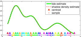
Figure 1: Visualization of the data, the shadow centers, and the associated KDE and ShKDE.

5 Analysis of Approximation Error

This section derives bounds on the MMD error for shadow densities, plus bounds on the difference between the eigenvalues and spectral projections of the operators associated to the original kernel matrix generated by KPCA, $K$, and the one generated by the shadow density, $\widetilde{K}$. The bounds demonstrate the claim that an accurate RSDE leads to an accurate eigendecomposition, since the bounds on the approximation error of the eigendecomposition are given in terms of the error of the approximated density estimate.

Consider a set of points $\mathcal{X}=\{x_{1},\dots,x_{n}\}$, sampled from the distribution ${p}$. Let the shadow centers be given by $\mathcal{C}=\{c_{1},\dots,c_{m}\}$, and define the data-to-center mapping $\alpha:\{1,\dots,n\}\to\{1,\dots,m\}$. The shadow quantized dataset generated from $\mathcal{X}$ is given by  $\vbox{\hrule height=0.25pt\kern 1.07639pt\hbox{\kern-1.99997pt$\mathcal{C}$\kern-1.99997pt}}=\{c_{\alpha(1)},\dots,c_{\alpha(n)}\}$.

Here, as in [20], kernels that satisfy the following inequality are considered,

$$(k(a,b)-k(c,d))^{2}\leq C_{\mathcal{X}}^{k}(\|a-b\|^{2}+\|b-d\|^{2}),$$ (18)

where $C_{\mathcal{X}}^{k}$ is a constant depending on $k$ and the sample set $\mathcal{X}$, and that can be written as

$$k(x,y)=\varphi\left(\frac{\|x-y\|^{p}}{\sigma^{p}}\right)$$ (19)

The Laplacian and Gaussian, in particular, satisfy (18) and (19) for $\varphi(s)=e^{-s}$. The constant $C_{\mathcal{X}}^{k}$ is $\frac{1}{\sigma^{2}}$ for the Laplacian, and is $\frac{1}{2\sigma^{2}}$ for the Gaussian [19].

The maximum mean discrepancy (MMD) is a distance measure between probability distributions in the Hilbert space $\mathcal{H}$ induced by the kernel $k$ [14]. The (biased) MMD is defined to be

$$\operatorname{MMD}(\mathcal{X},\mathcal{Y})_{b}^{2}:=\left\|\sum_{i=1}^{n}\frac{1}{n}\psi(x_{i})-\sum_{i=1}^{n}\frac{1}{n}\psi(y_{i})\right\|^{2}_{\mathcal{H}},$$ (20)

where the $b$ denotes bias and $\psi$ is the mapping from the input space $\mathbb{R}^{d}$ to $\mathcal{H}$, $\psi(x):=k(x,\cdot)$. The points $x_{i}\in\mathcal{X}$ and $y_{i}\in\mathcal{Y}$ are generated by probability distributions $p$ and $q$ respectively; both sets have the same number of elements. The MMD can be thought of as the squared $L^{2}$ distance between two KDEs of the form (8) (up to scaling factors induced by $\mathcal{H}$) [14]. Since the kernel in KPCA induces a smoothing effect on the samples from the true probability density ${p}$, a small value for the MMD between the KDE and an RSDE is indicative of the RSDE acting as an effective surrogate for ${p}$ in the KPCA space, thus generating an effective approximation to (2) via the use of Algorithm 1.

The theorem below bounds the difference in MMD between the KDE $\widehat{p}(x)$ and the ShDE $\widetilde{p}(x)$.

Theorem 5.1.

(MMD Worst Case Bound) Let $n$ be the number of samples, $\mathcal{X}$ be defined as above,     $\mathcal{C}$    be the quantized dataset, and let $k$ satisfy (19). Then

$$\operatorname{MMD}(\mathcal{X},\ \vbox{\hrule height=0.25pt\kern 1.07639pt\hbox{\kern-1.99997pt$\mathcal{C}$\kern-1.99997pt}}\ )_{b}\leq\sqrt{2\left(\kappa-\varphi\left(\frac{1}{\ell^{p}}\right)\right)}.$$ (21)

Proof.

Follows from (19) and (20) through the identity $\sum_{c_{i}\in\mathcal{C}}w_{i}\psi(c_{i})=\sum_{x_{i}\in\mathcal{X}}\psi(c_{\alpha(i)}),$ which gives the ShDE and the KDE the same cardinality, $n$. ∎

The ShDE+RSKPCA procedure creates a matrix $\widetilde{K}$ that acts as an $m\times m$ surrogate for the quantized kernel matrix $\vbox{\hrule height=0.25pt\kern 1.07639pt\hbox{\kern-1.99997pt$K$\kern-1.99997pt}}_{ij}=k(c_{\alpha(i)},c_{\alpha(j)}),\ \text{for}\ i,j=1\dots n$. Exploiting the quantization effect, the following theorems bound the eigenvalue difference between the two spectral decompositions and also the difference between the operators in $\mathcal{H}$ in terms of the Hilbert-Schmidt norm.

Theorem 5.2.

Let $k$ be such that (18) holds, and let $\lambda_{i}$ and $\bar{\lambda}_{i}$ be the eigenvalues of the normalized matrices $K$ and  $K$ respectively. Then

$$\sum_{i=1}^{n}(\lambda_{i}-\bar{\lambda}_{i})^{2}\leq 2C_{\mathcal{X}}^{k}\left(\frac{\sigma}{\ell}\right)^{2}.$$

Proof.

Follows from the Hoffman-Wielandt inequality and (18). ∎

Given a kernel function $k$ and $\mathcal{X}$, a finite dimensional operator $K_{n}:\mathcal{H}\to\mathcal{H}$ approximating the ideal operator (2) can be defined via

$$K_{n}(\cdot):=\frac{1}{n}\sum_{i=1}^{n}\langle\cdot,k_{x_{i}}\rangle_{\mathcal{H}}k_{x_{i}},$$ (22)

where $x_{i}\in\mathcal{X}$ and $\langle\cdot,k_{x_{i}}\rangle_{\mathcal{H}}$ projects the point onto the kernel function $k_{x_{i}}:=k(\cdot,x_{i})\in\mathcal{H}$ [10]. The operator can be used to bound the error in Hilbert-Schmidt norm between the empirical operators generated by KPCA and ShDE+RSKPCA.

Theorem 5.3.

Let $K_{n}$ and $\ \vbox{\hrule height=0.25pt\kern 1.07639pt\hbox{\kern-1.99997pt$K$\kern-1.99997pt}}_{n}$ be defined using (22) with $\mathcal{X}$ and     $\mathcal{C}$ , respectively. Then

$$\|K_{n}-\vbox{\hrule height=0.25pt\kern 1.07639pt\hbox{\kern-1.99997pt$K$\kern-1.99997pt}}_{n}\|_{\operatorname{HS}}\leq 2\kappa\sqrt{2\left(\kappa-\varphi\left(\frac{1}{\ell^{p}}\right)\right)}.$$ (23)

Proof.

Define the operators $K_{n}$ and $\ \vbox{\hrule height=0.25pt\kern 1.07639pt\hbox{\kern-1.99997pt$K$\kern-1.99997pt}}_{n}$ via the extrapolation (22) using $k_{x_{i}}$ and $k_{c_{\alpha(i)}}$ respectively, and define the kernel residual in $\mathcal{H}$ to be $\epsilon_{i}:=k_{x_{i}}-k_{c_{\alpha(i)}}$. Then

$$K_{n}-\vbox{\hrule height=0.25pt\kern 1.07639pt\hbox{\kern-1.99997pt$K$\kern-1.99997pt}}_{n} =\frac{1}{n}\sum_{i=1}^{n}\left(\langle\cdot,k_{x_{i}}\rangle_{\mathcal{H}}\epsilon_{i}+\langle\cdot,\epsilon_{i}\rangle_{\mathcal{H}}k_{c_{\alpha(i)}}\right),$$

leading to

$$\left\|K_{n}-\vbox{\hrule height=0.25pt\kern 1.07639pt\hbox{\kern-1.99997pt$K$\kern-1.99997pt}}_{n}\right\|_{\operatorname{HS}} \leq\left\|\frac{1}{n}\sum_{i=1}^{n}\langle\cdot,k_{x_{i}}\rangle_{\mathcal{H}}\epsilon_{i}\right\|_{\operatorname{HS}}+\left\|\frac{1}{n}\sum_{i=1}^{n}\langle\cdot,\epsilon_{i}\rangle_{\mathcal{H}}k_{c_{\alpha(i)}}\right\|_{\operatorname{HS}}.$$

Using the properties of the Hilbert-Schmidt norm, and the maximizer $\epsilon^{\prime}$ such that the centroid error $\|\epsilon_{i}\|_{\mathcal{H}}$ is largest, the theorem follows. ∎

Proposition 5.3 shows that the centroid error in $\mathcal{H}$ is the key to the performance of the learning algorithm, and that the error is controlled solely in terms of the parameter $\ell$. The independence of the performance from the weights shows that ShDE effectively learns the percentage of the data that needs to be retained based on the value of $\ell$, which is dependent on the kernel and not the data. Finally, $\ell$ controls both the MMD and operator approximations, implying that the density estimate used in the shadow density procedure is sensible for learning in the eigenspace. Using this result, the following theorem follows.

Theorem 5.4.

Let $K_{n}$ and $\vbox{\hrule height=0.25pt\kern 1.07639pt\hbox{\kern-1.99997pt$K$\kern-1.99997pt}}_{n}$ be symmetric positive (finite) Hilbert-Schmidt operator of $\mathcal{H}$ defined by (22), and assume that $K_{n}$ has simple nonzero eigenvalues $\lambda_{1}>\lambda_{2}>\dots>\lambda_{n}$. Let $D>0$ be an integer such that $\lambda_{D}>0,\ \delta_{D}=\frac{1}{2}\left(\lambda_{D}-\lambda_{D+1}\right)$. If $2\sqrt{\kappa}\|\epsilon^{\prime}\|_{\mathcal{H}}<\delta_{D}/2$, then

$$\|P^{D}(K_{n})-P^{D}(\vbox{\hrule height=0.25pt\kern 1.07639pt\hbox{\kern-1.99997pt$K$\kern-1.99997pt}}_{n})\|_{\operatorname{HS}}\leq\frac{2\sqrt{2\kappa\left(\kappa-\varphi\left(\frac{1}{\ell^{p}}\right)\right)}}{\delta_{D}},$$ (24)

where $P^{D}(A)$ denotes the projection onto the $D$-dimensional eigenspace of $A\in\operatorname{HS}(\mathcal{H})$ associated to the largest eigenvalues.

Proof.

Follows from Theorem 3 in [21] and Proposition 5.3. ∎

6 Experimental Results

This section demonstrates the effectiveness of RSKPCA on real-world data. Approximation accuracy tests include eigenembedding and classification tasks with the Gaussian kernel. The datasets used and the bandwidths chosen (via cross-validation) are given in Table 2. In the figures, $n_{t}$ refers to the number of the points the model is trained on. All of the comparison algorithms require specification of the reduced set size $m$. To compare, the shadow method is run with $\ell$ then the average of all $m$ achieved on the datasets determines the value $m$ for the other methods. Table 2 compares the training time and storage size (which relates to evaluation time). All comparisons are made with KPCA as the baseline. Speedup is relative to the equivalent KPCA execution time.

Eigenembedding comparison with Nyström methods.

This experiment demonstrates the fidelity of the eigenfunctions computed by ShDE+RSKPCA to those generated by KPCA. The capacity of generalization of the approximate eigenfunctions is tested. Using KPCA as the baseline, ShDE+RSKPCA is compared with three other methods: 1) subsampled KPCA with bases chosen via random uniform sampling, 2) the regular Nyström method with bases chosen via random uniform sampling, and 3) the density weighted Nyström (WNyström) method [20]. The experimental methodology is as follows. First, the KPCA model is trained on the entire dataset. Then, shadow, uniform, Nyström, and WNyström KPCA models are trained using $80\%$ of the data for $\ell\in[3.0,5.0]$, in increments of $0.1$. The reason $\ell=3.0$ is chosen as a lower bound for the Gaussian is because lower values of $\ell$ pick points that are no longer similar to the centroid, while $\ell>5$ generally results in a loss in training efficiency. The KPCA eigenfunction embedding is computed for the remaining $20\%$ of the data for all the models, with rank $r=5$. The embeddings are aligned with each other using the transform ${\rm argmin}_{A\in\mathbb{R}^{r\times r}}\|O-\tilde{O}A\|_{F}$, where $O$ is the matrix representing the KPCA embedding, and $\tilde{O}$ represents the approximate KPCA embedding. The Frobenius norm difference of the embeddings and eigenvalues, the training and testing speedup, and the amount of data retained are averaged over 50 runs for each $\ell$, and are shown in Figures 2 and 3 for the german and pendigits datasets. As expected, while subsampled KPCA is faster in the training stage, it performs worse than any other method, implying that an appropriate weighting is necessary to approximate the eigenfunctions of KPCA. For larger values of $\ell$, ShDE+RSKPCA always performs well when it comes to approximating the eigenvalues and eigenfunctions of the operator. In terms of eigenembedding accuracy, using ANOVA with a value of $\alpha=0.05$, ShDE+RSKPCA is better than the Nyström embeddings after $\ell=3.2(3.3)$ and no worse than the WNyström embeddings after $\ell=4.0(4.8)$ for pendigits (german), and asymptotically approaches the KPCA baseline. While slower than the Nyström method for training, ShDE+RSKPCA is faster than KPCA for training and achieves significant testing speedups. It does so by retaining a subset of the data via selection of $\ell$, c.f. Fig. 6(a,b).

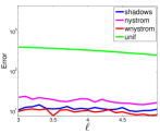
(a) Eigenvalue Deviation

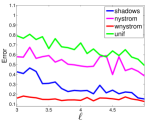
(b) Embedding Accuracy

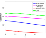
(c) Eigen speedup

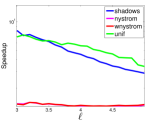
(d) Testing speedup

Figure 2: Eigenembedding comparison w/Nyström methods for german as $\ell$ is varied ($n_{t}=800$).

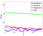
(a) Eigenvalue Deviation

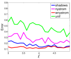
(b) Embedding Accuracy

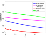
(c) Eigen speedup

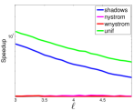
(d) Testing speedup

Figure 3: Eigenembedding comparison w/Nyström for pendigits as $\ell$ is varied ($n_{t}=2,800$).

Table 1: Datasets used.

german pendigits usps yale $n$ 1,000 3,500 9,298 5,768 dim 24 16 256 520 classes 2 10 10 10 $k$ 5 5 15 10 $\sigma$ 30 120 18 17

Table 2: Training cost and storage comparison.

ShDE+RSKPCA Nyström WNyström time $\mathcal{O}(mn+m^{3})$ $\mathcal{O}(mn+m^{3})$ $\mathcal{O}(mn+m^{3})$ space $\mathcal{O}(mr)$ $\mathcal{O}(nr)$ $\mathcal{O}(nr)$

KPCA classification comparison with Nyström methods.

This experiment examines the effectiveness of ShDE+RSKPCA for classification compared with the Nyström methods used previously. Classification utilizes the $k$-nn classifier with $k=3$, using $10$-fold cross-validation. The accuracy, training and testing speedups, and the percentage of data are reported. The results are shown in Figures 4 and 5 for the usps and yale methods respectively (none = KPCA). For the $k$-nn classification case, ShDE+RSKPCA has competitive accuracy with the Nyström methods, while providing significant training and testing speedups. The training speedup over the Nyström method in this case is because the eigenembedding of the data needs to be computed as part of the $k$-nn classifier training. Note that the data retained here, Fig. 6(c,d), is less than 10% for $\ell\in[3,5]$, implying noticeable speedup in the KPCA step of the classifier (during training and evaluation).

RSKPCA with different RSDE schemes.

RSKPCA is performed using alternative RSDEs to demonstrate the influence of the RSDE algorithm on accuracy, Figs. 7 and 8. Following [20], $k$-means provides a means to generate an RSDE at a time complexity of $\mathcal{O}(mn)$ (but tends to be slow due being iterative). Second, KDE paring [8] subsamples from the original dataset and computes the estimate from the reduced set, at an $\mathcal{O}(m)$ cost. Third, kernel herding is examined [5], which provides a mechanism to sample from a KDE using a nonlinear dynamical system. The samples are shown to be good representative samples. Their generation is $\mathcal{O}(n^{2}m)$. All of these algorithms require the user to provide the number $m$. It can be seen that the quality of the RSDE does influence the accuracy for small $\ell$, less so for larger $\ell$. The center selection schemes that lead to improved accuracy are costlier than ShDE, thus decreasing training gains. Evaluation speedup is the same for all methods.

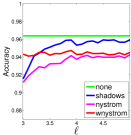
(a) Accuracy

(b) Training speedup

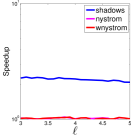
(c) Testing speedup

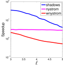
(d) Total speedup

Figure 4: Classification comparison w/Nyström for usps as $\ell$ is varied ($n_{t}=8,368$).

(a) Accuracy

(b) Training speedup

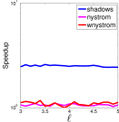
(c) Testing speedup

(d) Total speedup

Figure 5: Classification comparison w/Nyström methods for yale as $\ell$ is varied ($n_{t}=5,191$).

(a) german

(b) pendigits

(c) usps

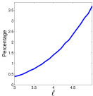
(d) yale

Figure 6: Percentage of data retained.

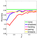
(a) Accuracy

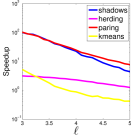
(b) Training speedup

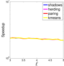
(c) Testing speedup

(d) Total speedup

Figure 7: Classification comparisons w/RSDEs for usps as $\ell$ is varied ($n_{t}=8,368$).

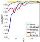
(a) Accuracy

(b) Training speedup

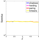
(c) Testing speedup

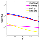
(d) Total speedup

Figure 8: Classification comparisons w/RSDEs for yale as $\ell$ is varied ($n_{t}=5,191$).

7 Conclusion

This paper presented (1) a reduced set KPCA algorithm for speeding up KPCA given a reduce set density estimate of the training data, and (2) a simple, efficient, single-pass algorithm for generating a suitable RSDE, called the shadow density estimate (ShDE), which relies on a user-selected parameter $\ell$. The spectral decomposition error was shown to be bounded and directly related to the bound of the empirical error of the ShDE. Through ShDE+RSKPCA, significant reductions in both training and evaluation time are achieved with minimal performance loss for large, redundant datasets. Competitive overall speedups and performance were achieved versus Nyström methods.

References

- [1] D. Achlioptas, F. McSherry, and B. Schölkopf. Sampling techniques for kernel methods. In NIPS.
- [2] O. Arif and P.A. Vela. Kernel map compression for speeding the execution of kernel-based methods. IEEE Transactions on Neural Networks, 22(6):870–879, 2011.
- [3] M. Belkin and P. Niyogi. Laplacian Eigenmaps for dimensionality reduction and data representation. Neural Computation, 15(6):1373–1396, June 2003.
- [4] Y. Bengio, P. Vincent, and J-F. Paiement. Learning eigenfunctions links Spectral Embedding and Kernel PCA. Neural Computation, 16(10):2197–2219, October 2004.
- [5] Y. Chen, M. Welling, and A. Smola. Super-samples from kernel herding. In Uncertainty in Artificial Intelligence, 2010.
- [6] R.R Coifman and S. Lafon. Diffusion maps. Applied and Computational Harmonic Analysis, 21:5–30, 2006.
- [7] P. Drineas and M.W. Mahoney. On the Nystrom method for approximating a gram matrix for improved kernel-based learning. Journal of Machine Learning Research, 6(10):2153–2175, October 2005.
- [8] D. Freedman and P. Kisilev. KDE Paring and a faster mean shift algorithm. SIAM Journal of Imaging Sciences, 3(4):878–903, March 2010.
- [9] J. Ham, D.D. Lee, S. Mika, and Bernhard Schölkopf. A kernel view of the dimensionality reduction of manifolds. In ICML, 2004.
- [10] L. Rosasco, M. Belkin, and E.D. Vito. On learning with integral operators. Joural of Machine Learning Research, 11:905–934, March 2010.
- [11] B. Schölkopf, S. Mika, C.J.C. Burges, P. Knirsch, K. Müller, G. Rätsch, and A.J. Smola. Input space versus feature space in kernel-based methods. IEEE Transactions on Neural Networks, 10(5):1000–1017, 1999.
- [12] B. Scholköpf, A. Smola, and R. Müller. Nonlinear component analysis as a kernel eigenvalue problem. Neural Computation, 10(5):1299–1319, July 1998.
- [13] J. Shawe-Taylor and N. Cristianini. Kernel Methods for Pattern Analysis. Cambridge University Press, New York, NY, USA, 2004.
- [14] A.J. Smola, A. Gretton, L. Song, and B. Scholkopf. A Hilbert space embedding for distributions. Algorithmic Learning Theory, 2007.
- [15] M. E. Tipping. Sparse kernel principal component analysis. In NIPS, pages 633–639, 2000.
- [16] X. Wang, P. Tino, M.A. Fardal, S. Raychaudhury, and A. Babul. Fast parzen window density estimator. In International Joint Conference on Neural Networks, pages 3267–3274, 2009.
- [17] L. Wasserman. All of Statistics. Springer, 2004.
- [18] C.K.I. Williams and M. Seeger. The effect of the input density distribution on kernel-based classifiers. In ICML, pages 1159–1166, 2000.
- [19] K. Zhang and J.T. Kwok. Improved nystrom low rank approximation and error analysis. In ICML, pages 1232–1239, 2008.
- [20] K. Zhang and J.T. Kwok. Density-weighted Nystrom method for computing large kernel eigensystems. Neural Computation, 21(1):1299–1319, January 2010.
- [21] L. Zwald and G. Blanchard. On the convergence of eigenspaces in kernel principal component analysis. In NIPS, 2005.