2+1-dimensional wormhole from a doublet of scalar fields

Abstract

We present a class of exact solutions in the framework of $2+1-$dimensional Einstein gravity coupled minimally to a doublet of scalar fields. Our solution can be interpreted upon tuning of parameters as an asymptotically flat wormhole as well as a particle model in $2+1-$dimensions.

I Introduction

Multiplets theory of real-valued scalar fields constitutes a model that naturally generalizes the theory of single scalar field model 1 . $\sigma-$Model 2 , the Higgs formalism 3 and global monopole theory 4 are just a few to be mentioned in this category. Extra fields amount always to extra degrees of freedom and richness in the underlying theory. The kinetic part of the Lagrangian in this approach  is proportional to $\left(\nabla\phi^{a}\right)^{2},$ (with $a,$ a symmetry group index) which is invariant under the symmetry transformations. In flat spacetime this makes a linear theory but in a curved spacetime intrinsic non-linearity automatically develops. Existence of an additional potential is employed as instrumental to apply spontaneous symmetry breaking in the generation of mass. Additional topological properties also are interesting subjects in this context.

Our aim in this study firstly, is to add new degrees of freedom to scalar fields with internal indices in the spacetime of $2+1-$dimensional gravity. This amounts to consider multiplets of scalar fields and obtain exact wormhole solutions in $2+1-$dimensions with non-zero curvature. $2+1-$dimensional wormholes were considered before 5 . In this particular dimension such a study with scalar doublets has not been conducted before. We are motivated in this line of thought mainly by the $2+1-$dimensional analogue of a Barriola-Vilenkin 4  type global monopole solution which is not any simpler than its $3+1-$dimensional counterpart 6 . We recall that the original idea of a spacetime wormhole, namely the Einstein-Rosen bridge 7 aimed to construct a geometrical model for an elementary particle. For the popularity of wormholes, however, we owe to the pioneering work of Morris and Thorne 8 .

Expectedly the invariance group in our case is $O\left(2\right)$ instead of $O\left(3\right).$ It should be added that in $2+1-$dimensions even the single scalar field solutions are very rare and restrictive 9 . This situation alone gives enough justification to search for alternatives such as the non-isotropic scalar multiplets. Secondly, we show that the solution obtained is a wormhole solution with the particular  red-shift function $\Phi\left(r\right)=0,$ leaving us with the shape function $b\left(r\right)$. It should be emphasized that vanishing of the red-shift function is not a choice but rather imposed as a result of the field equations. Our wormhole is powered by an exotic matter 10 and the scalar field doublet $\phi^{a}\left(r,\theta\right)$ is expressed in transcendental Lambert functions. When these are brought together our solution for the wormhole becomes supported by a phantom scalar field doublet. Wormholes with a phantom scalar in $3+1-$dimensions were studied in 11 . Phantom wormholes in $2+1-$dimensions were considered in 12 . Another interpretation for our solution can be considered a la’ Einstein and Rosen to represent a localized particle model in $2+1-$dimensions. We wish to comment that $2+1-$dimensional gravity gained enough prominence during recent decades all due to the discovery of a cosmological black hole 13 . This gave birth to the general consensus among relativists that the $2+1-$dimensional geometrical structures such as black holes and wormholes provide useful test-beds for understanding their higher dimensional cousins. Within this context we see certain advantages in studying and understanding better the $2+1-$dimensional wormhole solutions.

The organization of the paper is as follows. In Section II we introduce our action and derive the field equations. We solve and plot the metric function in Section III either as a wormhole or particle. Our conclusion in Section IV completes the paper.

II Action and field equations

The $2+1-$dimensional action in the Einstein gravity coupled to a scalar field, without cosmological constant and self interacting potential is given by ($16\pi G=c=1$)

$$S=\int d^{3}x\sqrt{-g}\left(R-\frac{\epsilon}{2}\left(\nabla\phi^{a}\right)^{2}\right)$$ (1)

in which $\epsilon=+1/-1$ corresponds to normal / phantom scalar field where $\phi^{a}$ is the doublet scalar field with $a=1,2$. The standard form of the line element for a wormhole in circularly symmetric $2+1-$dimensional spacetime is given by

$$ds^{2}=-e^{2\Phi}dt^{2}+\frac{1}{1-\frac{b\left(r\right)}{r}}dr^{2}+r^{2}d\theta^{2}.$$ (2)

Here $\Phi=\Phi\left(r\right)$ is the red-shift function and $b\left(r\right)$ is the shape function satisfying the so called flare-out conditions to which we shall refer in the sequel. Our doublet scalar field ansatz is given by

$$\phi^{a}=\eta f\left(r\right)\frac{x^{a}}{r},$$ (3)

where $x^{1}=r\cos\theta$ and $x^{2}=r\sin\theta,$ $\eta$ is a coupling constant and $f\left(r\right)$ is a real function of $r.$ This ansatz is well-known from the particle-like global monopole solution in the gravity coupled field theory model 4 . It admits topological properties and due to its angular dependence it exhibits non-isotropic properties in the radial plane. In particular the asymptotic behaviors are comparable with those of cosmic strings which are known to possess deficit angles. Such a model gives rise to lumpy structures in cosmic formations and naturally modifies all tests of general relativity ranging from planetary motion to the light bending. The reality of the model can only be tested by comparing geodesics of all kinds with the experimental data.

Considering the doublet field given in (3) one finds

$$\left(\nabla\phi^{a}\right)^{2}=\eta^{2}\left(\left(1-\frac{b}{r}\right)f^{\prime 2}+\frac{f^{2}}{r^{2}}\right)$$ (4)

such that after applying the variation of the action with respect to $f$ the field equation becomes

$$f^{\prime\prime}+\left(\Phi^{\prime}+\frac{2r-\left(b+rb^{\prime}\right)}{2r\left(r-b\right)}\right)f^{\prime}-\frac{f}{r\left(r-b\right)}=0.$$ (5)

We note that a prime stands for the derivative with respect to $r.$ Einstein’s equations are given as

$$G_{\mu}^{\nu}=T_{\mu}^{\nu}$$ (6)

for

$$T_{\mu}^{\nu}=\frac{\epsilon}{2}\left(\partial_{\mu}\phi^{a}\partial^{\nu}\phi^{a}-\frac{1}{2}\partial_{\rho}\phi^{a}\partial^{\rho}\phi^{a}\delta_{\mu}^{\nu}\right).$$ (7)

The latter implies

$$T_{t}^{t}=-\epsilon\frac{\eta^{2}}{4}\left(\left(1-\frac{b}{r}\right)f^{\prime 2}+\frac{1}{r^{2}}f^{2}\right),$$ (8)

$$T_{r}^{r}=\epsilon\frac{\eta^{2}}{4}\left(\left(1-\frac{b}{r}\right)f^{\prime 2}-\frac{1}{r^{2}}f^{2}\right)$$ (9)

and

$$T_{\theta}^{\theta}=-T_{r}^{r}.$$ (10)

Accordingly, Einstein’s equations read

$$\frac{b-rb^{\prime}}{2r^{3}}=-\epsilon\frac{\eta^{2}}{4}\left(\left(1-\frac{b}{r}\right)f^{\prime 2}+\frac{1}{r^{2}}f^{2}\right),$$ (11)

$$\frac{\left(r-b^{\prime}\right)\Phi^{\prime}}{r^{2}}=\epsilon\frac{\eta^{2}}{4}\left(\left(1-\frac{b}{r}\right)f^{\prime 2}-\frac{1}{r^{2}}f^{2}\right)$$ (12)

and

$$\frac{2r\left(r-b\right)\Phi^{\prime\prime}+2\Phi^{\prime}\left(r\left(r-b\right)\Phi^{\prime}+\frac{1}{2}\left(b-rb^{\prime}\right)\right)}{2r^{2}}=\\ -\epsilon\frac{\eta^{2}}{4}\left(\left(1-\frac{b}{r}\right)f^{\prime 2}-\frac{1}{r^{2}}f^{2}\right).$$ (13)

In the next section we shall find an exact solution for the four field equations given in (5), (11), (12) and (13).

III Exact solutions

The field equations admit an exact solution for $\Phi=0.$ The field equations, in this setting become

$$f^{\prime\prime}+\left(\frac{2r-\left(b+rb^{\prime}\right)}{2r\left(r-b\right)}\right)f^{\prime}-\frac{f}{r\left(r-b\right)}=0,$$ (14)

$$\frac{b-rb^{\prime}}{2r^{3}}=-\epsilon\frac{\eta^{2}}{4}\left(\left(1-\frac{b}{r}\right)f^{\prime 2}+\frac{1}{r^{2}}f^{2}\right)$$ (15)

and

$$\left(1-\frac{b}{r}\right)f^{\prime 2}-\frac{1}{r^{2}}f^{2}=0.$$ (16)

The last equation implies

$$b=\left(r-\frac{1}{r}\frac{f^{2}}{f^{\prime 2}}\right)$$ (17)

and upon substitution into (14) one finds that it is satisfied. Therefore the only equation left becomes

$$2rf^{\prime 2}-2ff^{\prime}-2rf^{\prime\prime}f+\epsilon\eta^{2}r^{2}ff^{\prime 3}=0$$ (18)

which can be rewritten as

$$\left(\frac{f}{rf^{\prime}}\right)^{\prime}=-\frac{1}{2}\epsilon\eta^{2}ff^{\prime}.$$ (19)

An integration yields

$$\frac{f}{rf^{\prime}}=-\frac{\epsilon\eta^{2}}{4}f^{2}+C_{1}$$ (20)

with the integration constant $C_{1}$. The resulting equation simply reads

$$\frac{dr}{r}=\left(-\frac{\epsilon\eta^{2}}{4}f+\frac{C_{1}}{f}\right)df$$ (21)

which is integrable as

$$\ln\left(\frac{r}{r_{0}}\right)=-\frac{\epsilon\eta^{2}}{8}f^{2}+C_{1}\ln f$$ (22)

with $r_{0}$ another integration constant. Finally, $f$ is found to be

$$f=\left(\frac{r}{r_{0}}\right)^{\xi}\exp\left[-\frac{1}{2}LW\left(-\frac{\epsilon\eta^{2}\xi}{4}\left(\frac{r}{r_{0}}\right)^{2\xi}\right)\right]$$ (23)

in which $\xi=\frac{1}{C_{1}}$ and $LW\left(x\right)$ is the Lambert-W function 14 . Using (23) we also find the exact form of $b\left(r\right)$ which is determined as

$$b=r\left[1-\frac{\left(1+LW\left(-\frac{\epsilon\eta^{2}\xi}{4}\left(\frac{r}{r_{0}}\right)^{2\xi}\right)\right)^{2}}{\xi^{2}}\right].$$ (24)

The only non-zero component of the energy momentum tensor is $T_{0}^{0}=-\rho$ in which the energy density is given by

$$\rho=-\frac{2}{r^{2}\xi}LW\left(-\frac{\epsilon\eta^{2}\xi}{4}\left(\frac{r}{r_{0}}\right)^{2\xi}\right).$$ (25)

In these solutions there are four parameters: $\eta$ and $\epsilon$ from the action and $r_{0}$ and $\xi=\frac{1}{C_{1}}$ as integration constants. Setting $\eta=0$ directly yields $\phi^{a}=0$ and $b\left(r\right)=\frac{1}{\xi^{2}}$ which corresponds to the flat spacetime. Due to the quadratic form of $\eta^{2}$, both in the action and in the solution, $\eta\lessgtr 0$ have similar contribution. Also, $r_{0}$ is a scale factor with dimension as $r$ and therefore we restrict $r_{0}>0.$ Unlike $\eta$, the sign of the other two parameters bring different features for the general solutions. Here we study each case separately.

III.1 $\epsilon=1,\xi>0$

The first setup corresponds to $\epsilon=1,\xi>0.$ In this setting, $f\left(r\right)$ is defined for $r<r_{c}=\left(2/\eta\sqrt{\xi e}\right)^{1/\xi}r_{0}$ and therefore the solution is bounded from above and we shall call it a particle model. In this confined model the particle is supported by normal matter with $\rho>0.$

III.2 $\epsilon=1,\xi<0$

The second setup for the two free parameters is considered as $\epsilon=1$ and $\xi<0$. In this case the line-element can be written as

$$ds^{2}=-dt^{2}+\frac{1}{B\left(r\right)}dr^{2}+r^{2}d\theta^{2}$$ (26)

where

$$B\left(r\right)=\frac{1}{\xi^{2}}\left(1+LW\left(-\frac{\eta^{2}\xi}{4}\left(\frac{r}{r_{0}}\right)^{2\xi}\right)\right)^{2}$$ (27)

which is positive for $r>0.$ For $r=0$ there exists a singularity while for large $r$, $B\left(r\right)$ asymptotes to $\frac{1}{\xi^{2}}.$ Therefore without loss of generality one may set $\xi=-1.$ (We note that unlike the $3+1-$dimensional spacetime where

$$ds^{2}=-dt^{2}+\xi^{2}dr^{2}+r^{2}\left(d\theta^{2}+\sin^{2}\theta d\phi^{2}\right)$$ (28)

is flat only if $\xi^{2}=1,$ in $2+1-$dimensions for any value of $\xi\neq 0$, the spacetime is flat.) In Fig. 1 we plot $B\left(r\right)$ in terms of $r$ for various values for $\eta$. The solution is supported by normal matter of doublet scalar field which is naked singular at $r=0$ and asymptotically flat. We observe from this figure that larger value of $\eta^{2}$ makes the spacetime more deviated from the flat spacetime corresponding to $\eta^{2}=0.$ Therefore the larger the $\eta^{2}$ the stronger the doublet scalar fields which results in stronger curvature. Having $\epsilon=1$ in the action makes the scalar fields physical and also $\xi<0$ makes the energy density $\rho>0.$ Therefore this solution represents a naked singular solution supported by normal doublet of scalar field which is asymptotically flat. This solution can also be interpreted as a particle model constructed from the doublet of scalar fields. To complete this part, we add that the field function $f\left(r\right)$ is well defined for $r>0$ and its asymptotic behaviors are

$$\lim_{r\rightarrow 0}f\left(r\right)=\infty$$ (29)

and

$$\lim_{r\rightarrow\infty}f\left(r\right)=0.$$ (30)

It is observed that the source of the field looks to be diverging at $r=0,$ where the spacetime is curved maximally and is singular.

Figure 1: $B\left(r\right)$ versus $r$ (Eq. (27)) for various values of $\eta=5.0,1.0,0.5,0.1$ and $0.0$ from top to bottom, respectively, with $\xi=-1,\epsilon=1,r_{0}=1.$

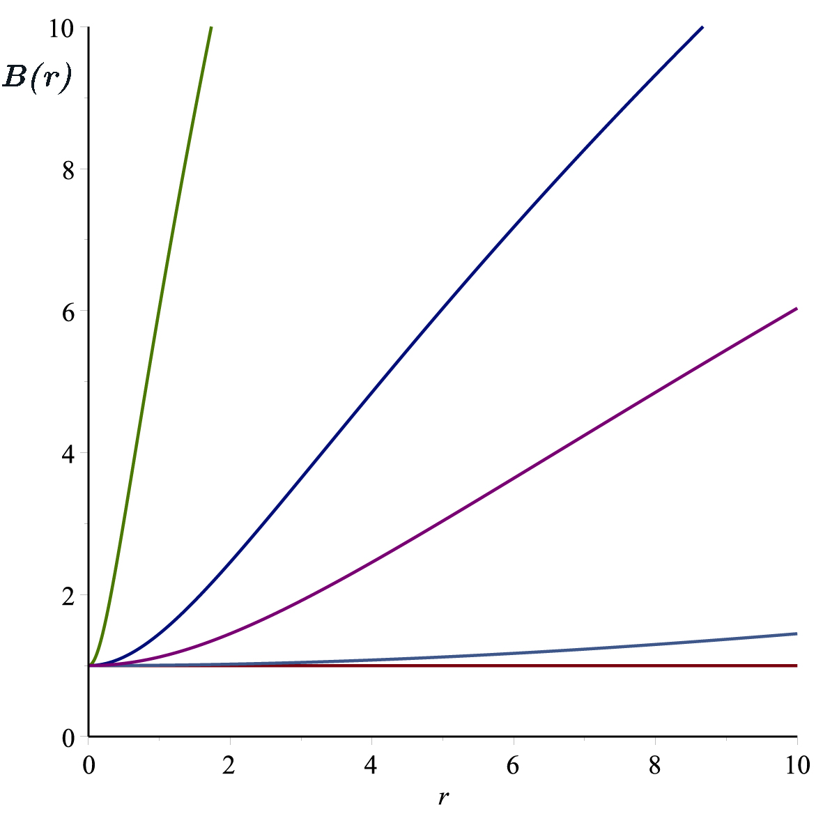
Figure 2: $B\left(r\right)$ versus $r$ (Eq. (27)) for various values of $\eta=5.0,1.0,0.5,0.1$ and $0.0$ from top to bottom, respectively, with $\xi=1,\epsilon=-1,r_{0}=1.$

Figure 3: (a) From top to bottom (Eqs. (35)-(38)); $K,$ $R_{\mu\nu}R^{\mu\nu},$ $\rho$ and $R$ versus $r>b_{0}$ (b) $B\left(r\right)$ (dashed) and $\eta f\left(r\right)$ (solid) in terms of $r$ for $r>b_{0}.$ For both we set $b_{0}=1,$ $\epsilon=-1$ and $\xi=-1.$

Figure 4: $B\left(r\right)$ versus $r$ from Eq. (27) for various values of $\eta=5.0,1.0,0.5,0.1$ and $0.0$ from bottom to top, respectively, with $\xi=-1,\epsilon=-1,r_{0}=1.$

III.3 $\epsilon=-1,\xi>0$

In this setting for $\epsilon=-1$ and $\xi>0$ the solution is exotic, supported by negative energy density. The field function $f\left(r\right)$ is well defined for $r>0,$ and while at $r=0$ it vanishes at large $r$ it diverges.

In Fig. 2 we plot $B\left(r\right)$ versus $r$ for different values of $\eta.$ The solution is supported by exotic matter / phantom doublet of scalar fields, which is flat near $r=0$ and non-asymptotically flat for $r\rightarrow\infty$. Larger value of $\eta^{2}$ makes the spacetime more deviated from the flat spacetime with $\eta^{2}=0.$ Note that the asymptotic behaviors of the solution at small $r$ and large $r$ in the present case look to be the opposite of the previous case. The two cases are still different solutions and by a change of variable, for instance $r\rightarrow\frac{1}{r},$ one can not obtain one from the other.

III.4 Wormhole solution for $\epsilon=-1,\xi<0$

Our last general setting addresses to the most interesting case where $\epsilon=-1,\xi<0$ and the solution represents a wormhole with a throat located at

$$b_{0}=r_{0}\left(\frac{e\eta^{2}\left|\xi\right|}{4}\right)^{\frac{1}{2\left|\xi\right|}}$$ (31)

in which $e$ stands for the natural base of logarithm. The wormhole is asymptotically flat with

$$\lim_{r\rightarrow\infty}B\left(r\right)=\frac{1}{\xi^{2}}$$ (32)

where we shall choose $\xi=-1.$ Both $b\left(r\right)$ and $f\left(r\right)$ are positively defined for $r>b_{0}$ and $b\left(r\right)$ satisfies the flare-out conditions i.e., i) $b(b_{0})=b_{0}$; and ii) for $r>b_{0}$, $rb^{\prime}<b$ such that the field function smoothly vanishes at infinity from its maximum value $\frac{\sqrt{2}}{\left|\eta\right|}$ at the throat. In terms of the throat radius one may write

$$f=\frac{2\left(\frac{b_{0}}{r}\right)^{\left|\xi\right|}}{\eta\sqrt{e\left|\xi\right|}}\exp\left[-\frac{1}{2}LW\left(\frac{-1}{e}\left(\frac{b_{0}}{r}\right)^{2\left|\xi\right|}\right)\right],$$ (33)

$$b=r\left(1-\frac{1}{\xi^{2}}\left[1+LW\left(\frac{-1}{e}\left(\frac{b_{0}}{r}\right)^{2\left|\xi\right|}\right)\right]^{2}\right)$$ (34)

with the scalar invariants given by

$$K=R_{\mu\nu\alpha\beta}R^{\mu\nu\alpha\beta}=\frac{16LW\left(\frac{-1}{e}\left(\frac{b_{0}}{r}\right)^{2\left|\xi\right|}\right)^{2}}{r^{4}\xi^{2}},$$ (35)

$$R_{\mu\nu}R^{\mu\nu}=\frac{8LW\left(\frac{-1}{e}\left(\frac{b_{0}}{r}\right)^{2\left|\xi\right|}\right)^{2}}{r^{4}\xi^{2}}$$ (36)

and

$$R=R_{\mu}^{\mu}=\frac{4LW\left(\frac{-1}{e}\left(\frac{b_{0}}{r}\right)^{2\left|\xi\right|}\right)}{r^{2}\left|\xi\right|}.$$ (37)

The only non-zero component of the energy momentum tensor is the $tt$ component which is given by

$$T_{t}^{t}=-\rho=-\frac{2LW\left(\frac{-1}{e}\left(\frac{b_{0}}{r}\right)^{2\left|\xi\right|}\right)}{r^{2}\left|\xi\right|}.$$ (38)

Let’s add that on the range of $r$ i.e., $r\geq b_{0}$ all of the quantities given above are finite and asymptotically they vanish. In addition one finds

$$\lim_{r\rightarrow b_{0}^{+}}f=\frac{2}{\eta\sqrt{\left|\xi\right|}},\text{ \ }\lim_{r\rightarrow b_{0}^{+}}b=b_{0}$$ (39)

$$\lim_{r\rightarrow b_{0}^{+}}\rho=-\frac{2}{b_{0}^{2}\sqrt{\left|\xi\right|}},\text{ \ }\lim_{r\rightarrow b_{0}^{+}}K=\frac{16}{b_{0}^{4}\xi^{2}}$$ (40)

and

$$\lim_{r\rightarrow b_{0}^{+}}R_{\mu\nu}R^{\mu\nu}=\frac{8}{b_{0}^{4}\xi^{2}},\text{ \ }\lim_{r\rightarrow b_{0}^{+}}R=-\frac{4}{b_{0}^{2}\left|\xi\right|}.$$ (41)

In Fig. 3a we plot the scalars given above to show that they are finite everywhere and in Fig. 3b the curve of energy density $\rho$ together with the corresponding metric function $B\left(r\right)$ are displayed. The energy density is negative everywhere but finite, indicating the wormhole is supported by exotic matter 10 . In Fig. 4 we plot $B\left(r\right)$ versus $r$ for different values of $\eta$ with fixed values for $\xi=-1$ and $r_{0}=1$ (Note that with $r_{0}=1$ and different values for $\eta$ the throat $b_{0}$ is not fixed). The magnitude of $\eta$ plays a critical role to form the throat of the wormhole such that the larger value for $\eta$ implies larger size of the throat.

III.5 $\xi=0$ and $\xi=\infty$

Among the possible values for $\xi$ the case with $\xi=0$ corresponds to $f=1$ and consequently to the flat space solution. In contrast to that, when $\xi\rightarrow\infty$ the solution becomes (this can be seen from (22) when $C_{1}=0$)

$$f^{2}=-\frac{8}{\epsilon\eta^{2}}\ln\left(\frac{r}{r_{0}}\right)$$ (42)

so that

$$b=r\left(1-4\left(\ln\frac{r}{r_{0}}\right)^{2}\right)$$ (43)

and

$$ds^{2}=-dt^{2}+\frac{dr^{2}}{\left(2\ln\frac{r}{r_{0}}\right)^{2}}+r^{2}d\theta^{2}.$$ (44)

This line element has the following scalar invariants

$$R=R_{\mu}^{\mu}=-\frac{8\ln\frac{r}{r_{0}}}{r^{2}}$$ (45)

$$K=R_{\mu\nu\alpha\beta}R^{\mu\nu\alpha\beta}=\frac{64\ln^{2}\frac{r}{r_{0}}}{r^{4}}$$ (46)

and

$$R_{\mu\nu}R^{\mu\nu}=\frac{32\ln^{2}\frac{r}{r_{0}}}{r^{4}}.$$ (47)

It is seen clearly that $r=0$ is a spacetime singularity while at $r=r_{0}$ it is regular. This metric can’t be interpreted as a wormhole since from (43) as $r>r_{0}$ the sign of $b\left(r\right)$ turns negative which is in contrast to the definition of a wormhole. The only non-zero component of the energy-momentum tensor is given by

$$T_{t}^{t}=\frac{4\ln\frac{r}{r_{0}}}{r^{2}},$$ (48)

with a divergent energy density at the origin given by

$$\rho=-T_{t}^{t}$$ (49)

IV Conclusion

For a number of reasons in recent decades the lower / higher dimensional curved spacetimes received much popularity. Our aim in this paper was to consider a doublet of non-isotropic scalar fields $\phi^{a}\left(r,\theta\right)$ transforming under the group $O\left(2\right).$ We present parametric solutions for such a system to determine the underlying $2+1-$dimensional spacetime. Our solution involves the restrictive condition of vanishing red-shift function. By making $g_{tt}=-1$ leaves us with a single metric function $g_{rr}=\frac{1}{B\left(r\right)}$ besides $\phi^{a}\left(r,\theta\right).$ Once the red-shift function vanishes our solution loses its chance to represent a black hole. However, the wormhole and particle interpretations are admissible and as a matter of fact this summarizes the contribution made in this paper. Our only metric function as well as the doublet scalar functions are expressed in terms of a Lambert function which is tabulated extensively in the literature. The source supporting our wormhole turns out to be exotic which persists to be a deep-rooted problem in general. We wish to remark finally that in order to overcome this problem of exoticity we proposed recently one resolution, which is to change the circular topological character of the throat 15 .

References

- (1) C. Barceloand M. Visser, Class. Quantum Grav. 17, 3843 (2000); S.-W. Kim and S. P. Kim, Phys. Rev. D 58, 087703 (1998); O. Hauser, R. Ibadov, B. Kleihaus and J. Kunz, Phys. Rev. D 89, 064010 (2014); A. Anabalón, D. Astefanesei and R. Mann, JHEP 10, 184 (2013); T. Torii and H.-aki Shinkai, Phys. Rev. D 88, 064027 (2013).
- (2) M. Gell-Mann and M. Lévy, Il Nuovo Cimento 16, 705 (1960).
- (3) P. W. Higgs, Phys. Rev. Lett. 13, 508 (1964).
- (4) M. Barriola and A. Vilenkin, Phys. Rev. Lett. 63, 341 (1989).
- (5) G.P. Perry, R.B. Mann, Gen. Relativ. Grav. 24, 305 (1992); S. W. Kim, H. J. Lee, S. K. Kim and J. Yang, Phys. Lett. A 183, 359 (1993); M. S. R. Delgaty and R. B. Mann, Int. J. Mod. Phys. D 4, 231 (1995); W. T. Kim, J. J. Oh and M. S. Yoon, Phys. Rev. D 70, 044006 (2004); F. Rahaman, A. Banerjee and I. Radinschi, Int. J. Theor. Phys. 51, 1680 (2012); A. Banerjee, Int. J. Theor. Phys. 52, 2943 (2013); C. Bejarano, E.F. Eiroa, and C. Simeone, Eur. Phys. J. C 74, 3015 (2014).
- (6) S. H. Mazharimousavi and M. Halilsoy, arXiv:1408.3008 ”Global Monopole-BTZ black hole”.
- (7) A. Einstein and N. Rosen, Phys. Rev. 48, 73 (1935).
- (8) M. S. Morris and K. S. Thorne, Am. J. Phys. 56, 395 (1988).
- (9) K. S. Virbhadra, Pramana 44, 317 (1995).
- (10) M. Visser, S. Kar and N. Dadhich, Phys. Rev. Lett. 90, 201102 (2003); S.V. Bolokhov, K.A. Bronnikov and M.V. Skvortsova, Class. Quantum Grav. 29, 245006 (2012).
- (11) K. A. Bronnikov, S. V. Chervon and S.V. Sushkov, Grav.Cosmol. 15, 241 (2009).
- (12) M. Jamil, M. U. Farooq, Int. J. Theor. Phys. 49, 835 (2010).
- (13) M. Bañados, C. Teitelboim, J. Zanelli, Phys. Rev. Lett. 69, 1849 (1992). M. Bañados, M. Henneaux, C. Teitelboim and J. Zanelli, Phys. Rev. D 48, 1506 (1993). C. Martinez, C. Teitelboim and J. Zanelli, Phys. Rev. D 61, 104013 (2000). S. Carlip, Quantum Gravity in 2 + 1-Dimensions, Cambridge University Press, 1998.
- (14) R. M. Corless, ”On the Lambert W Function”: University of Waterloo, Computer Science Department, 1993.
- (15) S. H. Mazharimousavi and M. Halilsoy, Eur. Phys. J. C 75, 81 (2015).