Sampling-based Learning Control for Quantum Systems with Uncertainties

Abstract

Robust control design for quantum systems has been recognized as a key task in the development of practical quantum technology. In this paper, we present a systematic numerical methodology of sampling-based learning control (SLC) for control design of quantum systems with uncertainties. The SLC method includes two steps of “training” and “testing”. In the training step, an augmented system is constructed using artificial samples generated by sampling uncertainty parameters according to a given distribution. A gradient flow based learning algorithm is developed to find the control for the augmented system. In the process of testing, a number of additional samples are tested to evaluate the control performance where these samples are obtained through sampling the uncertainty parameters according to a possible distribution. The SLC method is applied to three significant examples of quantum robust control including state preparation in a three-level quantum system, robust entanglement generation in a two-qubit superconducting circuit and quantum entanglement control in a two-atom system interacting with a quantized field in a cavity. Numerical results demonstrate the effectiveness of the SLC approach even when uncertainties are quite large, and show its potential for robust control design of quantum systems.

I Introduction

The control and manipulation of quantum phenomena lie at the heart of developing practical quantum technologies, and the exploration of quantum control theory and methods is drawing wide interests from scientists and engineers [1]-[4]. In the development of practical quantum technologies, robustness has been recognized as a key performance measure since the existence of uncertainties and noises is unavoidable in the modeling and control process for real quantum systems [5]-[8]. For example, the chemical shift may not be exactly known in the model of a spin system in nuclear magnetic resonance (NMR) [9], [10]. In a superconducting quantum circuit, there exist possible fluctuations in the coupling energy of a Josephson junction [11], [12]. In the dipole approximation for a molecular system interacting with laser fields, imprecision in the model parameters is unavoidable [13]. It is also common that there exist errors in control pulses or fields applied to quantum systems. Hence, it is important to develop systematic robust design methods for the analysis and synthesis of quantum systems with uncertainties. Several methods have been proposed for the robust control of quantum systems [14]-[26]. For example, James et al. [14] have formulated and solved an $H^{\infty}$ controller synthesis problem for a class of quantum linear stochastic systems. Adiabatic techniques (e.g., STIRAP - stimulated Raman adiabatic passage) [27]-[31] have been widely applied to robust control problems of quantum systems when the adiabatic limit can be satisfied. Optimized composite pulses have been applied in NMR to improve robustness performance [9], [32]. A noise filtering approach has been presented to enhance robustness in quantum control [33]. A sequential convex programming method has been proposed for designing robust quantum gates [34]. A sliding mode control approach has been presented to deal with Hamiltonian uncertainties in two-level quantum systems [15], [16].

In classical (non-quantum) control systems, feedback control is the dominant method for robust control design. Feedback control (including measurement-based feedback control and coherent feedback control) has been applied to some quantum systems for improved control performance [3], [35]-[40]. However, open-loop control is more practical than feedback control for most quantum systems with current technology considering the small time scales and measurement backaction in the quantum domain [34]. Several open-loop control strategies have been presented to design robust control laws for specific quantum systems. For example, dynamical decoupling has been developed for control design of quantum systems with uncertainties [41]-[43]. Existing results showed that control fields designed by learning have the property of robustness [34], [44], [45]. Recently, Zhang et al. [46] employed a gradient-based algorithm to design robust control pulses for electron shuttling. They considered that parameter uncertainties exist in the energy difference when an electron is transported along a chain of donors. An effective optimization algorithm has been developed to find robust control pulses by discretizing the uncertainty range and deriving the gradient of an aggregate fidelity with respect to sinusoidal control fields [46].

In this paper, we present a systematic numerical methodology of sampling-based learning control (SLC) for robust design of quantum systems with uncertainties. Sampling-based learning control was first presented for control design of inhomogeneous quantum ensembles where the SLC method includes two steps of “training” and “testing” [47]. A generalized system is constructed from some samples with different values of the inhomogeneous parameters in the training step and a control field is learned through a gradient flow based optimization algorithm. The control is evaluated using additional samples for some possible values of the inhomogeneous parameters. The results showed that the SLC approach can find an effective control law to drive the members in an inhomogeneous ensemble to a given target state with high fidelity. In this paper, we contribute a systematic SLC method with specific learning algorithms for the robust control of quantum systems with uncertainties. In particular, we generate artificial samples by sampling the uncertainty parameters in the system model and construct an augmented system using these samples in the training step [48]. Then a gradient flow based learning and optimization algorithm is developed to learn a control law with desired performance for the augmented system. In the process of testing, we test a number of samples of the uncertainties to evaluate the control performance. The SLC method is applied to three significant examples of quantum robust control. The first example is a three-level quantum system that is found widely in natural atoms and artificial atoms [49]. A problem of state preparation is investigated when uncertainties exist in the three-level system. In the second example, we consider superconducting quantum circuits which have been recognized as promising candidates for quantum information processing due to their advantages of scalability and design flexibility (see, e.g., [50], [51], [52], [53]). In particular, we employ the SLC method to learn a robust control law that can be applied to a two-qubit superconducting circuit for generating quantum entanglement. The third example investigates the application of the SLC approach to the robust control of quantum entanglement in a two-atom system interacting with a quantized field in a cavity [54], [55]. Numerical results show that the SLC method is effective for robust control design of these classes of quantum systems with uncertainties.

This paper is organized as follows. Section II formulates the quantum control problem. Section III presents the sampling-based learning control approach and introduces a gradient flow based learning algorithm. Numerical results on control design in three-level quantum systems are presented in Section IV. The SLC method is applied to robust entanglement generation in a two-qubit superconducting circuit in Section V. In Section VI, the SLC approach is used to learn a robust control law for a two-atom system interacting with a quantized field in a cavity. Concluding remarks are presented in Section VII.

II Problem formulation of quantum robust control

We focus on a finite-dimensional quantum system that can be approximated as a closed system and whose state is described using a complex vector $|\psi\rangle$ or a density operator $\rho=|\psi\rangle\langle\psi|$ in an underlying Hilbert space. The evolution of its state $|\psi(t)\rangle$ can be described by the following Schrödinger equation:

$$\left\{\begin{array}[]{l}\frac{d}{dt}|{\psi}(t)\rangle=-\frac{i}{\hbar}H(t)|\psi(t)\rangle\\ \ |\psi(0)\rangle=|\psi_{0}\rangle.\\ \end{array}\right.$$ (1)

The dynamics of the system are governed by a time-dependent Hamiltonian of the form [56]

$$H(t)=H_{0}+H_{c}(t)=H_{0}+\sum_{m=1}^{M}u_{m}(t)H_{m},$$ (2)

where $H_{0}$ is the free Hamiltonian of the system, $H_{c}(t)=\sum_{m=1}^{M}u_{m}(t)H_{m}$ is the time-dependent control Hamiltonian that represents the interaction of the system with the external fields $u_{m}(t)$ (scalar functions), and the $H_{m}$ are Hermitian operators through which external controls couple to the system.

The solution of (1) is given by $\displaystyle|\psi(t)\rangle=U(t)|\psi_{0}\rangle$, where the propagator $U(t)$ satisfies

$$\left\{\begin{array}[]{c}\frac{d}{dt}U(t)=-\frac{i}{\hbar}H(t)U(t),\\ \ U(0)=I.\\ \end{array}\right.$$ (3)

For an ideal model, there exist no uncertainties in (2). However, for a practical quantum system, the existence of uncertainties is unavoidable due to external disturbances, imprecise models and errors in control fields. In this paper, we suppose that the system Hamiltonian has the following form

$$H_{\Theta}(t)=f_{0}(\theta_{0})H_{0}+\sum_{m=1}^{M}f_{m}(\theta_{m})u_{m}(t)H_{m}.$$ (4)

We have denoted $\Theta=(\theta_{0},\theta_{1},\dots,\theta_{M})$ and the functions $f_{j}(\theta_{j})$ ($j=0,1,\dots,M$) characterize possible uncertainties. For example, $f_{0}(\theta_{0})$ corresponds to uncertainties in the free Hamiltonian (e.g., due to chemical shift in NMR). $f_{m}(\theta_{m})$ can characterize possible multiplicative noises in the control fields or imprecise parameters in the dipole approximation. When the $f_{m}(\theta_{m})$ are allowed to be time-dependent, the corresponding uncertainties may originate from time-varying errors in the control fields. For example, the time-dependent non-Markovian noise in the control field considered in [57] can be described using the model. It is also straightforward to include additive noises in control fields by slightly modifying (4). We assume that $f_{j}(\theta_{j})$ are continuous functions of $\theta_{j}$ and the parameters $\theta_{j}$ could be time-dependent and $\theta_{j}\in[1-E_{j},1+E_{j}]$. For simplicity, we assume the uncertainty bounds $E_{0}=\dots=E_{j}=\dots=E_{M}=E$ are all equal in this paper. We assume that the nominal values of $\theta_{j}$ are 1 and the fluctuations of the uncertainty parameters $\theta_{j}$ are $2E$ (where $E\in[0,1]$). The objective is to design the controls $\{u_{m}(t),m=1,2,\ldots,M\}$ to steer the quantum system with uncertainties from an initial state $|\psi_{0}\rangle$ to a target state $|\psi_{\text{target}}\rangle$ with high fidelity. The fidelity between two quantum states $|\psi_{1}\rangle$ and $|\psi_{2}\rangle$ is defined as [58], [59]:

$$F(|\psi_{1}\rangle,|\psi_{2}\rangle)=|\langle\psi_{1}|\psi_{2}\rangle|.$$ (5)

The control performance is described by a performance function $J(u)$ for each control strategy $u=\{u_{m}(t),m=1,2,\ldots,M\}$. The control problem can then be formulated as a maximization problem as follows:

$$\begin{split}\displaystyle\max_{u}\ \ &J(u):=\max_{u}\mathbb{E}|\langle\psi(T)|\psi_{\text{target}}\rangle|^{2}\\ \text{s.t.}\ \ &\frac{d}{dt}|\psi(t)\rangle=-\frac{i}{\hbar}H_{\Theta}(t)|\psi(t)\rangle,\ |\psi(0)\rangle=|\psi_{0}\rangle\\ &H_{\Theta}(t)=f_{0}(\theta_{0})H_{0}+\sum_{m=1}^{M}f_{m}(\theta_{m})u_{m}(t)H_{m},\\ &\textrm{ with }\theta_{j}\in[1-E,1+E],~{}t\in[0,T].\end{split}$$ (6)

Note that $J(u)$ depends implicitly on the control $u$ through the Schrödinger equation and $\mathbb{E}(\cdot)$ denotes the expectation with respect to the uncertainty parameters $\Theta=(\theta_{0},\theta_{1},\dots,\theta_{M})$.

III Sampling-based learning control method

Gradient-based methods [4], [60], [61] have been successfully applied to search for optimal solutions to a variety of quantum control problems, including theoretical and laboratory applications. In this paper, a gradient-based learning method is employed to optimize the control fields for quantum systems with uncertainties. However, it is impossible to directly calculate the derivative of $J(u)$ since there exist uncertainties and some parameters in the model are unknown. Hence, we present a systematic numerical methodology of sampling-based learning control which includes two steps of “training” and “testing”. In the training step, some artificial samples are generated through sampling the uncertainty parameters to construct an augmented system and a learning algorithm is developed to find an optimal control strategy for the augmented system. Then the designed control law is applied to additional samples to test and evaluate the control performance in the testing step.

III-A Sampling-based learning control

In the training step, we first generate $N$ samples through sampling the uncertainty parameters according to a given probability distribution (e.g., the uniform distribution). We could choose any of the combination $(\theta_{0n_{0}},\theta_{1n_{1}},\dots,\theta_{Mn_{M}})$ of the sampled parameters $\{\theta_{j},j=0,1,\ldots,M\}$, where $\theta_{jn_{j}}$ is a possible value of the uncertainty parameter $\theta_{j}$, $n_{j}=1,\dots,N_{j}$ and $N_{j}$ is the number of samples of the parameter $\theta_{j}$ ($j=0,1,\ldots,M$). The total number of potential samples is $N=\prod_{j=0}^{M}N_{j}$. We denote these different sample systems as $\{n\}\ (n=1,2,\ldots,N)$ and $\Theta_{n}\in\{(\theta_{0n_{0}},\theta_{1n_{1}},\dots,\theta_{Mn_{M}})|n_{j}=1,\dots,N_{j}\}$. With these samples, we can construct an augmented system as follows

$$\frac{d}{dt}\left(\begin{array}[]{c}|{\psi}_{1}(t)\rangle\\ |{\psi}_{2}(t)\rangle\\ \vdots\\ |{\psi}_{N}(t)\rangle\\ \end{array}\right)=-\frac{i}{\hbar}\left(\begin{array}[]{c}H_{\Theta_{1}}(t)|\psi_{1}(t)\rangle\\ H_{\Theta_{2}}(t)|\psi_{2}(t)\rangle\\ \vdots\\ H_{\Theta_{N}}(t)|\psi_{N}(t)\rangle\\ \end{array}\right),$$ (7)

where $H_{\Theta_{n}}(t)=f_{0}(\theta_{0n_{0}})H_{0}+\sum_{m}f_{m}(\theta_{mn_{m}})u_{m}(t)H_{m}$ with $n=1,2,\dots,N$. The performance function for the augmented system is defined by

$$J_{N}(u):=\frac{1}{N}\sum_{n=1}^{N}J_{\Theta_{n}}(u)=\frac{1}{N}\sum_{n=1}^{N}|\langle\psi_{n}(T)|\psi_{\text{target}}\rangle|^{2}.$$ (8)

The task of the training step is to find a control strategy $u^{*}$ that maximizes the performance function defined in Eq. (8). We will develop a gradient flow based learning algorithm to solve this optimization problem in an iterative way [47], [48]. Assume that the performance function is $J_{N}(u^{0})$ with an initial control strategy $u^{0}=\{u^{0}_{m}(t)\}$. We can apply the gradient flow method to obtain an (approximate) optimal control strategy $u^{*}=\{u^{*}_{m}(t)\}$. It is clear that we may take $u^{*}$ as an approximate optimal control solution when $J_{N}(u)\rightarrow 1$. For the nominal system (without uncertainties), the quantum control landscape theory [45] has shown that there are no local maxima in the optimization problem for closed quantum systems when they are controllable and the critical points of their control landscapes are regular (for details, see, e.g., [4], [45]). For the augmented system, it may be also possible to use a similar method to the quantum landscape theory to prove the optimal characteristics. Numerical results in this paper show that a gradient method can be used to achieve excellent performance in finding an approximate optimal solution. The detailed gradient flow algorithm will be presented in Subsection III-B.

As for the issue of choosing $N$ samples, we generally choose them according to possible distributions of the uncertainty parameters $\theta_{j}\in[1-E,1+E]$. The basic motivation of the proposed sampling-based approach is to design the control law using some artificial samples instead of unknown uncertainties. Therefore, it is necessary to choose the set of samples that are representatives of these uncertainty parameters.

For example, we consider the case with two uncertainty parameters $\theta_{0}$ and $\theta_{1}$. If the distributions of both $\theta_{0}$ and $\theta_{1}$ are uniform, we may choose equally spaced samples for $\theta_{0}$ and $\theta_{1}$. For example, the intervals $[1-E,1+E]$ for $\theta_{0}$ and $[1-E,1+E]$ for $\theta_{1}$ are divided into $N_{0}+1$ and $N_{1}+1$ subintervals, respectively, where $N_{0}$ and $N_{1}$ are usually positive odd numbers. Then the number of samples is $N=N_{0}N_{1}$, and $\Theta_{n}=(\theta_{0n_{0}},\theta_{1n_{1}})$ is chosen from the set of sample points

$$\Theta_{n}\in\{(\theta_{0n_{0}},\theta_{1n_{1}}): \theta_{0n_{0}}=1-E+\frac{(2n_{0}-1)E}{N_{0}},\ \ \ \ \ \ \ \ \ \ \ \ \$$

$$\theta_{1n_{1}}=1-E+\frac{(2n_{1}-1)E}{N_{1}}),\ \ \ \ \ \ \ \ \ \ \ \$$

$$n_{0}\in\{1,\ldots,N_{0}\},\ n_{1}\in\{1,\ldots,N_{1}\}\}.$$ (9)

In practical applications, the numbers of $N_{0}$ and $N_{1}$ can be chosen by experience or through numerical computation. As long as the augmented system can model the quantum system with uncertainties and is effective to find the optimal control strategy, we prefer to choose small numbers for $N_{0}$ and $N_{1}$ to speed up the training process and simplify the augmented system. Numerical results show that five or seven samples for each uncertainty parameter are enough to achieve excellent performance.

In the testing step, we apply the optimized control $u^{*}$ obtained in the training step to a large number of additional samples obtained through randomly sampling the uncertainty parameters. The control performance is evaluated for each sample in terms of the fidelity $F(|\psi(T)\rangle,|\psi_{\text{target}}\rangle)$ between the final state $|\psi(T)\rangle$ and the target state $|\psi_{\text{target}}\rangle$. If the fidelity for all the tested samples is satisfactory, we accept the designed control law and end the control design process. Otherwise, we go back to the training step to find another optimized control strategy by changing the settings (e.g., restarting the training step with a new initial control strategy or a new set of samples).

III-B Gradient flow based learning algorithm

To find an optimal control strategy $u^{*}=\{u^{*}_{m}(t),(t\in[0,T]),m=1,2,\ldots,M\}$ for the augmented system (7), a good choice is to follow the direction of the gradient of $J_{N}(u)$ as an ascent direction so as to speed up the learning process. For ease of notation, we present the method for the case $M=1$. We introduce a time-like variable $s$ to characterize different control strategies $u^{(s)}(t)$. Then the gradient flow in the control space can be defined as

$$\frac{du^{(s)}}{ds}=\nabla J_{N}(u^{(s)}),$$ (10)

where $\nabla J_{N}(u)$ denotes the gradient of $J_{N}$ with respect to the control $u$. If $u^{(s)}$ is the solution of (10) starting from an arbitrary initial condition $u^{(0)}$, then the value of $J_{N}$ is increasing along $u^{(s)}$, i.e., $\frac{d}{ds}J_{N}(u^{(s)})\geq 0$. In other words, starting from an initial guess $u^{0}$, we solve the following initial value problem

$$\left\{\begin{split}&\frac{du^{(s)}}{ds}=\nabla J_{N}(u^{(s)})\\ &u^{(0)}=u^{0}\\ \end{split}\right.$$ (11)

in order to find a control strategy which maximizes $J_{N}$. This initial value problem can be solved numerically by using a forward Euler method over the $s$-domain, i.e.,

$$u(s+\triangle s,t)=u(s,t)+\triangle s\nabla J_{N}(u^{(s)}).$$ (12)

For practical applications, we present an iterative approximation version of the above algorithm to find the optimal controls $u^{*}(t)$ in an iterative learning way, where we use $k$ as an index of iterations instead of the variable $s$ and denote the control at iteration step $k$ as $u^{k}(t)$. Equation (12) can be rewritten as

$$u^{k+1}(t)=u^{k}(t)+\eta_{k}\nabla J_{N}(u^{k}),$$ (13)

where $\eta_{k}$ is the updating step (learning rate) for the $k$th iteration. Using (8), we also have

$$\nabla J_{N}(u)=\frac{1}{N}\sum_{n=1}^{N}\nabla J_{\Theta_{n}}(u).$$ (14)

Recall that $J_{\Theta}(u)=|\langle\psi_{\Theta}(T)|\psi_{\textrm{target}}\rangle|^{2}$ and $|\psi_{\Theta}(\cdot)\rangle$ satisfies

$$\frac{d}{dt}|\psi_{\Theta}\rangle=-\frac{i}{\hbar}H_{\Theta}(t)|\psi_{\Theta}\rangle,\quad|\psi_{\Theta}(0)\rangle=|\psi_{0}\rangle.$$ (15)

We now derive an expression for the gradient of $J_{\Theta}(u)$ with respect to the control $u$ by using a first order perturbation. Let $\delta\psi(t)$ be the modification of $|\psi(t)\rangle$ induced by a perturbation of the control from $u(t)$ to $u(t)+\delta u(t)$. By keeping only the first order terms, we obtain the equation satisfied by $\delta\psi$:

$$\begin{split}\frac{d}{dt}\delta\psi=&-\frac{i}{\hbar}\left(f_{0}(\theta_{0})H_{0}+u(t)f_{1}(\theta_{1})H_{1}\right)\delta\psi\\ &-\frac{i}{\hbar}\delta u(t)f_{1}(\theta_{1})H_{1}|\psi_{\Theta}(t)\rangle,\\ \delta\psi(0)=&0.\end{split}$$

Let $U_{\Theta}(t)$ be the propagator corresponding to (15). Then, $U_{\Theta}(t)$ satisfies

$$\frac{d}{dt}U_{\Theta}(t)=-\frac{i}{\hbar}H_{\Theta}(t)U_{\Theta}(t),\quad U(0)=I.$$

Therefore,

$$\delta\psi(T)=-\frac{i}{\hbar}U_{\Theta}(T)\int_{0}^{T}\delta u(t)U_{\Theta}^{\dagger}(t)f_{1}(\theta_{1})H_{1}|\psi_{\Theta}(t)\rangle dt\ \ \ \ \$$

$$\ =-\frac{i}{\hbar}U_{\Theta}(T)\int_{0}^{T}U_{\Theta}^{\dagger}(t)f_{1}(\theta_{1})H_{1}U_{\Theta}(t)\delta u(t)dt~{}|\psi_{0}\rangle.$$ (16)

Using (16), we compute $J_{\Theta}(u+\delta u)$ as follows

$$J_{\Theta}(u+\delta u)-J_{\Theta}(u)\ \ \ \ \ \ \ \ \ \ \ \ \ \ \ \ \ \ \ \ \ \ \ \ \ \ \ \ \ \ \ \ \ \ \ \ \ \$$

$$\approx 2\Re\left(\langle\psi_{\Theta}(T)|\psi_{\textrm{target}}\rangle\langle\psi_{\textrm{target}}|\delta\psi(T)\right)\ \ \ \ \ \ \ \ \ \ \ \ \ \ \ \ \ \ \$$

$$= 2\Re\left(-i\langle\psi_{\Theta}(T)|\psi_{\textrm{target}}\rangle\langle\psi_{\textrm{target}}|\int_{0}^{T}V(t)\delta u(t)dt~{}|\psi_{0}\rangle\right)$$

$$= \int_{0}^{T}2\Im\left(\langle\psi_{\Theta}(T)|\psi_{\textrm{target}}\rangle\langle\psi_{\textrm{target}}|V(t)|\psi_{0}\rangle\right)\delta u(t)dt,\ \ \$$ (17)

where $\Re(\cdot)$ and $\Im(\cdot)$ denote, respectively, the real and imaginary parts of a complex number, and $V(t)=U_{\Theta}(T)U_{\Theta}^{\dagger}(t)f_{1}(\theta_{1})H_{1}U_{\Theta}(t)$.

Recall also that the definition of the gradient implies that

$$J_{\Theta}(u+\delta u)-J_{\Theta}(u)= \langle\nabla J_{\Theta}(u),\delta u\rangle_{L^{2}([0,T])}+o(\|\delta u\|)$$

$$= \int_{0}^{T}\nabla J_{\Theta}(u)\delta u(t)dt+o(\|\delta u\|).$$ (18)

Therefore, by identifying (17) with (18), we obtain

$$\nabla J_{\Theta}(u)=2\Im\left(\langle\psi_{\Theta}(T)|\psi_{\textrm{target}}\rangle\langle\psi_{\textrm{target}}|V(t)|\psi_{0}\rangle\right).$$ (19)

The gradient flow method can be generalized to the case with $M>1$ as shown in Algorithm 1. For a termination criterion of the iterative learning process, we use the following: if the change of the performance function for $100$ consecutive iterations is less than a given small threshold $\epsilon>0$, i.e., $|J(u^{k+100})-J(u^{k})|<\epsilon$, we end the learning process. In this paper we choose $\epsilon=10^{-4}$ for all numerical experiments.

Algorithm 1 Gradient flow based iterative learning

1:Set the index of iterations $k=0$

2:Choose a set of arbitrary controls $u^{k=0}=\{u_{m}^{0}(t),\ m=1,2,\ldots,M\},t\in[0,T]$

3:repeat (for each iterative process)

4:     repeat (for each training sample $n=1,2,\ldots,N$)

5:         Compute the propagator $U_{\Theta_{n}}^{k}(t)$ with the control strategy $u^{k}(t)$

6:     until  $n=N$

7:     repeat (for each control $u_{m}\ (m=1,2,\ldots,M)$ of the control vector $u$)

8:         $\delta_{m}^{k}(t)=\frac{2}{N}\sum^{N}_{n=1}\Im\left(\langle\psi_{n}(T)|\rho_{\textrm{target}}V^{k}_{\Theta_{n}}(t)|\psi_{0}\rangle\right)$ where $\rho_{\textrm{target}}=|\psi_{\textrm{target}}\rangle\langle\psi_{\textrm{target}}|$, $V^{k}_{\Theta_{n}}(t)=U^{k}_{\Theta_{n}}(T)(U_{\Theta_{n}}^{k}(t))^{\dagger}f_{m}(\theta_{mn_{m}})H_{m}U^{k}_{\Theta_{n}}(t)$ and $n_{m}\in\{1,2,\dots,N_{m}\}$

9:         $u_{m}^{k+1}(t)=u_{m}^{k}(t)+\eta_{k}\delta_{m}^{k}(t)$

10:     until  $m=M$

11:     $k=k+1$

12:until  the learning process ends

13:The optimal control strategy $u^{*}=\{u_{m}^{*}\}=\{u_{m}^{k}\},\ m=1,2,\ldots,M$

In practical applications, it is usually difficult to find the numerical solution to a time varying continuous control strategy $u(t)$ using Algorithm 1. In simulation, we usually divide the time interval $[0,T]$ equally into a number of smaller time intervals $\triangle t$ and assume that the controls are constant within each $\triangle t$. Instead of $t\in[0,T]$, the time index will be $t_{w}=wT/W$, where $W=T/\triangle t$ and $w=0,1,\ldots,W$.

In the following three sections, we apply the SLC method to three examples. The first example is the state preparation in a general three-level quantum system where the main focus is on demonstrating the SLC method. We assume that there are no constraints on the control fields and the uncertainty parameters have uniform distributions or time-varying distributions. In the second example, we consider entanglement generation in superconducting quantum circuits. We use some practical models and relevant parameters in the literature. Bounded control fields and truncated Gaussian distributions for uncertainty parameters are assumed. The third example considers the application of the SLC method to a two-atom system interacting with a quantized field.

IV State preparation in three-level quantum systems

In this section, we demonstrate the application of the proposed SLC method to robust state preparation in a $V$-type three-level quantum system with uncertainties. $V$-type three-level systems are a typical class of quantum systems in atomic physics. Some natural and artificial atoms can be described by a $V$-type three-level model [49]. State preparation is an essential task in quantum information processing [58]. For example, specific quantum states are required to be prepared for initialization in quantum computation and transfer in quantum communication. It is important to achieve robust preparation of these specific states for practical applications of quantum technology. For simplicity, we assume no constraints on the external controls and use atomic units (i.e., setting $\hbar=1$) in this section. The aim is to show how to apply the proposed SLC method for robust control design of quantum systems with uncertainties.

IV-A State preparation in a $V$-type quantum system

We consider a $V$-type quantum system and demonstrate the SLC design process. Assume that the initial state is $|\psi(t)\rangle=c_{1}(t)|1\rangle+c_{2}(t)|2\rangle+c_{3}(t)|3\rangle$. Let $C(t)=(c_{1}(t),c_{2}(t),c_{3}(t))$ where the $c_{i}(t)$’s are complex numbers. We have

$$i\dot{C}(t)=(f_{0}(\theta_{0})H_{0}+\sum_{m=1}^{M}f_{m}(\theta_{m})u_{m}(t)H_{m})C(t).$$ (20)

We take $H_{0}=\textrm{diag}(1.5,1,0)$ and choose $H_{1}$, $H_{2}$, $H_{3}$ and $H_{4}$ as follows [62]:

$$H_{1}=\left(\begin{array}[]{ccc}0&1&0\\ 1&0&0\\ 0&0&0\\ \end{array}\right),\ H_{2}=\left(\begin{array}[]{ccc}0&-i&0\\ i&0&0\\ 0&0&0\\ \end{array}\right),\ \ \ \ \ \ \ \ \ \ \ \ \ \ \$$

$$\ H_{3}=\left(\begin{array}[]{ccc}0&0&1\\ 0&0&0\\ 1&0&0\\ \end{array}\right),\ \ \ H_{4}=\left(\begin{array}[]{ccc}0&0&-i\\ 0&0&0\\ i&0&0\\ \end{array}\right).$$ (21)

For simplicity, we assume $f_{m}(\theta_{m})=f(\vartheta)$ for all $m=1,2,3,4$ and $f_{0}(\theta_{0})=f_{0}(\vartheta)$. After we sample the uncertainty parameters, every sample can be described as follows:

$$\left(\begin{array}[]{c}\dot{c_{1}}(t)\\ \dot{c_{2}}(t)\\ \dot{c_{3}}(t)\\ \end{array}\right)=\left(\begin{array}[]{ccc}-1.5f_{0}(\vartheta)i&G_{1}(\vartheta)&G_{2}(\vartheta)\\ G^{*}_{1}(\vartheta)&-f_{0}(\vartheta)i&0\\ G^{*}_{2}(\vartheta)&0&0\\ \end{array}\right)\left(\begin{array}[]{c}c_{1}(t)\\ c_{2}(t)\\ c_{3}(t)\\ \end{array}\right)$$ (22)

where $G_{1}(\vartheta)=f(\vartheta)[u_{2}(t)-iu_{1}(t)]$, $G_{2}(\vartheta)=f(\vartheta)[u_{4}(t)-iu_{3}(t)]$ and $\vartheta\in[1-E,1+E]$ . $E\in[0,1]$ is a given constant and $G^{*}$ is the complex conjugate of $G$.

To construct an augmented system for the training step of the SLC design, we choose $N$ training samples (denoted as $n=1,2,\ldots,N$) through sampling the uncertainties as follows:

$$\left(\begin{array}[]{c}\dot{c}_{1,n}(t)\\ \dot{c}_{2,n}(t)\\ \dot{c}_{3,n}(t)\\ \end{array}\right)=B_{n}(t)\left(\begin{array}[]{c}c_{1,n}(t)\\ c_{2,n}(t)\\ c_{3,n}(t)\\ \end{array}\right),$$ (23)

$$B_{n}(t)=\left(\begin{array}[]{ccc}-1.5f_{0}(\vartheta_{n})i&G_{1}(\vartheta_{n})&G_{2}(\vartheta_{n})\\ G^{*}_{1}(\vartheta_{n})&-f_{0}(\vartheta_{n})i&0\\ G^{*}_{2}(\vartheta_{n})&0&0\\ \end{array}\right),$$

where $G_{1}(\vartheta_{n})=f(\vartheta_{n})[u_{2}(t)-iu_{1}(t)]$, $G_{2}(\theta_{n})=f(\vartheta_{n})[u_{4}(t)-iu_{3}(t)]$. For simplicity, we assume that $f_{0}(\vartheta)=f(\vartheta)=\vartheta$ have uniform distributions over $[1-E,1+E]$. Now the objective is to find a robust control strategy $u(t)=\{u_{m}(t),m=1,2,3,4\}$ to drive the quantum system from $|\psi_{0}\rangle=|1\rangle$ (i.e., $C_{0}=(1,0,0)$) to $|\psi_{\text{target}}\rangle=\frac{1}{\sqrt{2}}(|2\rangle+|3\rangle)$ (i.e., $C_{\text{target}}=(0,\frac{1}{\sqrt{2}},\frac{1}{\sqrt{2}})$).

If we write (23) as $\dot{C}_{n}(t)=B_{n}(t)C_{n}(t)$ ($n=1,2,\ldots,N$), we can construct the following augmented system

$$\left(\begin{array}[]{c}\dot{C}_{1}(t)\\ \dot{C}_{2}(t)\\ \vdots\\ \dot{C}_{N}(t)\\ \end{array}\right)=\left(\begin{array}[]{cccc}B_{1}(t)&0&\cdots&0\\ 0&B_{2}(t)&\cdots&0\\ \vdots&\vdots&\ddots&\vdots\\ 0&0&\cdots&B_{N}(t)\\ \end{array}\right)\left(\begin{array}[]{c}C_{1}(t)\\ C_{2}(t)\\ \vdots\\ C_{N}(t)\\ \end{array}\right).$$ (24)

For this augmented system, we use the training step to learn an optimal control strategy $u(t)$ to maximize the following performance function

$$J(u)=\frac{1}{N}\sum_{n=1}^{N}|\langle C_{n}(T)|C_{\text{target}}\rangle|^{2}.$$ (25)

Now we employ Algorithm 1 to find an optimal control strategy $u^{*}(t)=\{u^{*}_{m}(t),m=1,2,3,4\}$ for the augmented system. Then we apply the optimal control strategy to additional samples to evaluate the performance of the control strategy.

IV-B Numerical results

For numerical experiments on a $V$-type quantum system, we use the parameter settings listed as follows: The initial state $|\psi_{0}\rangle=|1\rangle$ and the target state $|\psi_{\text{target}}\rangle=\frac{1}{\sqrt{2}}(|2\rangle+|3\rangle)$; The end time is $T=5$ and the total time duration $[0,T]$ is equally discretized into $W=200$ time intervals with each time interval $\Delta t=(t_{w}-t_{w-1})|_{w=1,2,\ldots,W}=T/W=0.025$; The learning rate is $\eta_{k}=0.2$; The control strategy is initialized with $u^{k=0}(t)=\{u^{0}_{m}(t)=\sin t,m=1,2,3,4\}$.

First, we assume that there exists only the uncertainty $f_{0}(\vartheta)$ (i.e., $f(\vartheta)\equiv 1$), $E=0.21$ and $f_{0}(\vartheta)$ has a uniform distribution in the interval $[0.79,1.21]$. To construct an augmented system for the training step, we use the training samples for this $V$-type quantum system defined as follows

$$\left\{\begin{split}&f_{0}(\vartheta_{n})=1-0.21+\frac{0.21(2n-1)}{7},\\ &f(\vartheta_{n})=1,\\ \end{split}\right.$$ (26)

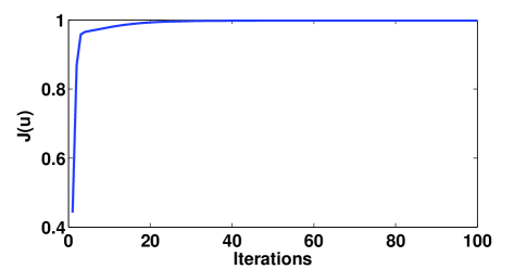
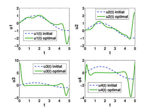
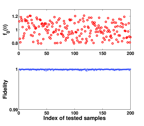
where $n=1,2,\ldots,7$. The training performance for the augmented system is shown in Fig. 1. It is clear that the learning process converges to a quite accurate stage very quickly. The optimal control strategy is demonstrated in Fig. 2, which is compared with the initial one. To test the optimal control strategy obtained from the training step, we choose $200$ samples obtained by sampling the uncertainty $f_{0}(\vartheta)$ according to a uniform distribution and demonstrate the testing performance in Fig. 3. For the 200 tested samples, an average fidelity of 0.9999 is achieved.

Figure 1: Training performance to find the optimal control strategy by maximizing $J(u)$ for the $V$-type quantum system with only uncertainty $f_{0}(\vartheta)$ where $f_{0}(\vartheta)\in[0.79,1.21]$.

Figure 2: The learned optimal control strategy with maximized $J(u)$ for the $V$-type quantum system with only the uncertainty $f_{0}(\vartheta)$ where $f_{0}(\vartheta)\in[0.79,1.21]$.

Figure 3: The testing performance (with respect to fidelity) of the learned optimal control strategy for the $V$-type quantum system with only uncertainty $f_{0}(\vartheta)$ where $f_{0}(\vartheta)\in[0.79,1.21]$. For the 200 tested samples, the average fidelity is 0.9999.

Now, we consider the more general case where there exist the uncertainties $f_{0}(\vartheta)$ and $f(\vartheta)$. Assume $E=0.21$, $f_{0}(\vartheta)=1-\vartheta_{0}\cos t$, $f(\vartheta)=1-\vartheta\cos t$, and both $\vartheta_{0}$ and $\vartheta$ have uniform distributions on the interval $[-0.21,0.21]$. To construct an augmented system for the training step, we use the training samples defined as follows

$$\left\{\begin{split}&f_{0}(\vartheta_{n})=1-0.21+\frac{0.21(2\text{fix}(n/7)-1)}{7},\\ &f(\vartheta_{n})=1-0.21+\frac{0.21(2\text{mod}(n,7)-1)}{7},\\ \end{split}\right.$$ (27)

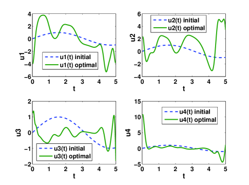
where $n=1,2,\ldots,49$, $\text{fix}(x)=\max\{z\in\mathbb{Z}|z\leq x\}$, $\text{mod}(n,7)=n-7z\ (z\in\mathbb{Z}\ \text{and}\ \frac{n}{7}-1<z\leq\frac{n}{7})$ and $\mathbb{Z}$ is the set of integers. The algorithm converges after around 9000 iterations and the optimal control strategy is presented in Fig. 4. To test the optimal control strategy obtained in the training step, we randomly choose $200$ samples by uniformly sampling the uncertainties $\vartheta_{0}$ and $\vartheta$ and an average fidelity of 0.9961 is achieved. However, if we use only one sample (i.e., the nominal system) for training to obtain a control law, the testing performance shows a 0.9152 average fidelity. These numerical results show that the proposed SLC method using an augmented system for training is effective for control design of quantum systems with uncertainties.

Figure 4: The learned optimal control strategy with maximized $J(u)$ for the $V$-type quantum system with the uncertainties $f_{0}(\vartheta)$ and $f(\vartheta)$ where $f_{0}(\vartheta)=1-\vartheta_{0}\cos t$, $f(\vartheta)=1-\vartheta\cos t$, and both $\vartheta_{0}$ and $\vartheta$ have uniform distributions on the interval $[-0.21,0.21]$.

V Robust entanglement generation in quantum superconducting circuits

Superconducting quantum circuits based on Josephson junctions are macroscopic circuits which can behave quantum mechanically like artificial atoms [50]-[53]. These artificial atoms can be used to test the laws of quantum mechanics on macroscopic systems and also offer a promising way to realize qubits in quantum information technology [11]. Superconducting quantum circuits have been recognized as promising candidates for quantum information processing due to their advantages of scalability and design flexibility. They have been widely investigated theoretically and experimentally in recent years [49], [63]-[70]. Superconducting qubits can be controlled by adjusting external parameters such as currents, voltages and microwave photons, and the coupling between two superconducting qubits can be turned on and off at will [50]. In practical applications, the existence of noise (including extrinsic and intrinsic) and inaccuracies (e.g., inaccurate operation in the coupling between qubits) in superconducting quantum circuits is unavoidable. In this section, we apply the SLC method to robust control design for a superconducting circuit system with uncertainties.

In superconducting quantum circuits, two typical classes of qubits are flux qubits and charge qubits which correspond to different ratios between the Josephson coupling energy $E_{J}$ and the charging energy $E_{C}$ (For a brief introduction to superconducting quantum circuits, see, e.g., [51], [69]). The simplest charge qubit is based on a small superconducting island (called a Cooper-pair box) coupled to the outside world through a weak Josephson junction and driven by a voltage source through a gate capacitance within the charge regime (i.e., $E_{C}\gg E_{J}$) [51]. In practical applications, the Josephson junction in the charge qubit is usually replaced by a dc superconducting quantum interference device (SQUID) with low inductance to make it easier to control the qubit. When we concentrate on a voltage range near a degeneracy point, the Hamiltonian of a superconducting charge qubit can be described as follows

$$H=F_{z}(V_{g})\sigma_{z}-F_{x}(\Phi)\sigma_{x}$$ (28)

where $F_{z}(V_{g})$ is related to the charging energy $E_{C}$ and this term can be adjusted through external parameters such as the voltage $V_{g}$, $F_{x}(\Phi)$ corresponds to a controllable term including different control parameters such as the flux $\Phi$ in the SQUID, and the Pauli matrices $\sigma=(\sigma_{x},\sigma_{y},\sigma_{z})$ with

$$\sigma_{x}=\begin{pmatrix}0&1\\ 1&0\\ \end{pmatrix},\ \ \ \ \sigma_{y}=\begin{pmatrix}0&-i\\ i&0\\ \end{pmatrix},\ \ \ \ \sigma_{z}=\begin{pmatrix}1&0\\ 0&-1\\ \end{pmatrix}.$$ (29)

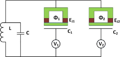
In this section, we consider the coupled two-qubit circuit in [69] where an LC-oscillator is used to couple two charge qubits (see Fig. 5). Each qubit is realized by a Cooper-pair box with Josephson coupling energy $E_{Ji}$ and capacitance $C_{Ji}$ ($i=1,2$). Each Cooper-pair box is biased by an applied voltage $V_{i}$ through a gate capacitance $C_{i}$ ($i=1,2$). The Hamiltonian of the coupled charge qubits can be described as [69]

$$\begin{split}H=&F_{z}(V_{1})\sigma^{(1)}_{z}\otimes I^{(2)}+F_{z}(V_{2})I^{(1)}\otimes\sigma^{(2)}_{z}\\ &-F_{x}(\Phi_{1})\sigma^{(1)}_{x}\otimes I^{(2)}-F_{x}(\Phi_{2})I^{(1)}\otimes\sigma^{(2)}_{x}\\ &-\chi(t)\sigma^{(1)}_{y}\otimes\sigma^{(2)}_{y}\end{split}$$ (30)

where $A^{(j)}$ denotes an operation $A$ on the qubit $j$ and $\otimes$ denotes the tensor product. Let $u_{1}(t)=F_{z}(V_{1})/\hbar$, $u_{2}(t)=F_{z}(V_{2})/\hbar$, $u_{3}(t)=F_{x}(\Phi_{1})/\hbar$, $u_{4}(t)=F_{x}(\Phi_{2})/\hbar$, $u_{5}(t)=\chi(t)/\hbar$. For simplicity, we assume the uncertainty parameters $f_{m}(\theta_{m})=\theta_{m}$ for all $m=1,2,3,4,5$. The Hamiltonian for the practical system can be described as

$$\begin{split}H/\hbar=&\theta_{1}u_{1}(t)\sigma^{(1)}_{z}\otimes I^{(2)}+\theta_{2}u_{2}(t)I^{(1)}\otimes\sigma^{(2)}_{z}\\ &-\theta_{3}u_{3}(t)\sigma^{(1)}_{x}\otimes I^{(2)}-\theta_{4}u_{4}(t)I^{(1)}\otimes\sigma^{(2)}_{x}\\ &-\theta_{5}u_{5}(t)\sigma^{(1)}_{y}\otimes\sigma^{(2)}_{y}\end{split}$$ (31)

where $\theta_{m}\in[1-E,1+E]$ ($m=1,2,3,4,5$).

For practical systems, $E_{J}$ could be around $10$ GHz and $E_{C}$ could be around $100$ GHz (e.g., the experiment in [67] used $E_{J1}=13.4\ \text{GHz}$, and $E_{C2}=152\ \text{GHz}$). In (31), we assume $u_{1}(t)\in[0,50.2]\ \text{GHz}$, $u_{2}(t)\in[0,50.2]\ \text{GHz}$, $u_{3}(t)\in[0,11.1]\ \text{GHz}$, $u_{4}(t)\in[0,11.1]\ \text{GHz}$, $|u_{5}(t)|\leq 0.5\ \text{GHz}$, and the operation time $T=2\ \text{ns}$. As an example, we let the task be to generate a maximally entangled state $|\psi_{\text{target}}\rangle=\frac{1}{\sqrt{2}}(|g_{1},g_{2}\rangle+|e_{1},e_{2}\rangle)$, where $|g_{j}\rangle$ and $|e_{j}\rangle$ denote the ground state and the excited state of qubit $j$, respectively. In quantum information, we usually use $|0\rangle$ (or $|1\rangle$) to denote $|g\rangle$ (or $|e\rangle$).

Quantum entanglement is a unique quantum phenomenon that occurs when quantum subsystems are generated or interact in ways such that the quantum state of each subsystem cannot be described independently [58], [71], [72]. Quantum entanglement shows nonclassical correlation and has been demonstrated as an important physical resource in quantum cryptography, quantum communication and quantum computation [58], [73]. We may use concurrence to measure how entangled a two-qubit state is [74]. For a two-qubit state $\rho$, let $\rho^{*}$ denote the complex conjugate of $\rho$, $\tilde{\rho}=(\sigma_{y}\otimes\sigma_{y})\rho^{*}(\sigma_{y}\otimes\sigma_{y})$ and $R=\sqrt{\sqrt{\rho}\tilde{\rho}\sqrt{\rho}}$. Let $\lambda_{1},\lambda_{2},\lambda_{3},\lambda_{4}$ be the eigenvalues of $R$ in decreasing order. The concurrence is defined as

$$\mathcal{C}(\rho)\equiv\max(0,\lambda_{1}-\lambda_{2}-\lambda_{3}-\lambda_{4}).$$

Let $\theta_{1}=\theta_{2}$, $\theta_{3}=\theta_{4}$, $\theta_{j}\in[0.79,1.21]$. In the training step, we uniformly select 7 values for each uncertainty parameter to generate samples for constructing an augmented system. In the testing step, we assume $\theta_{j}$ has a truncated Gaussian distribution. We also assume $|\psi_{0}\rangle=|g_{1},g_{2}\rangle$.

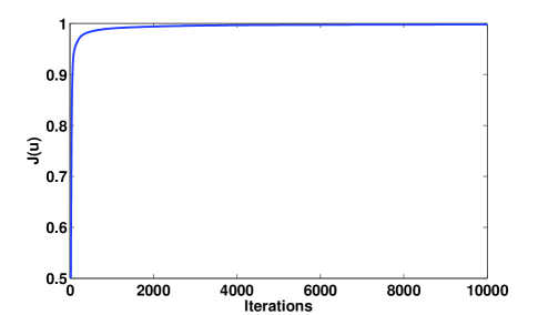
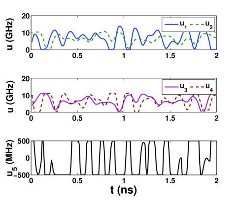
In numerical experiments, we divide $t\in[0,2]\ \text{ns}$ equally into $200$ time intervals. The control fields are initialized as: $u_{1}(0)=u_{2}(0)=u_{3}(0)=u_{4}(0)=\sin t+5\ \text{GHz}$, $u_{5}(0)=0.25\sin t\ \text{GHz}$. Assume the control fields satisfy $|u_{j}(t)|\leq V$. During the learning process, if the calculated control $u_{j}^{k}\geq V$ using the gradient algorithm, we let $u_{j}^{k}=V$. Similarly, if the calculated control $u_{j}^{k}\leq-V$, we let $u_{j}^{k}=-V$. The learning algorithm converges after about $9800$ iterations and the performance is shown in Fig. 6. A set of optimal control fields is shown in Fig. 7. Then the learned optimal control fields are applied to 2000 samples that are generated through selecting different values of uncertainty parameters according to the truncated Gaussian distribution with mean $\mu=1$ and standard deviation $\nu=0.07$ within the interval of $[1-3\nu,1+3\nu]=[0.79,1.21]$. The average concurrence is obtained from 2000 samples. When $\theta_{i}\in[0.79,1.21]$, the testing process (using 2000 randomly selected samples) shows that the average fidelity is 0.9992 and the average concurrence is 0.9981. Hence, the learned control fields can still drive the system to a maximally entangled state with high concurrence when the uncertainty parameters have $42\%$ fluctuations.

Figure 5: Two charge qubits coupled to a common LC-oscillator.

Figure 6: Training performance to find the optimal control strategy by maximizing $J(u)$ for coupled qubits via an LC-oscillator when the uncertainty bound is $E=0.21$.

Figure 7: The learned control field for the problem of coupled qubits via an LC-oscillator when the uncertainty bound is $E=0.21$.

VI Robust entanglement control between two atoms in a cavity

VI-A The system

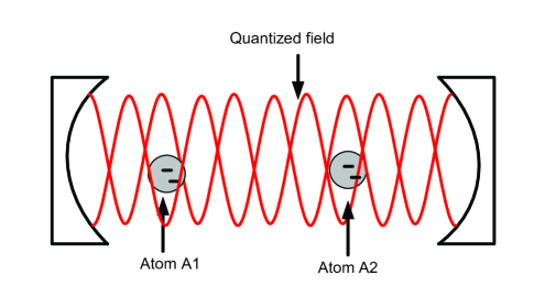
In this section, we apply the SLC method to a quantum system consisting of two two-level atoms interacting with a quantized field in an optical cavity (see Fig. 8) or in a microwave cavity. This model has been wieldy used in experimental quantum optics and quantum information [54, 55, 75, 76, 77]. The two-qubit system can be represented using four basis vectors $|g_{1},g_{2}\rangle$, $|e_{1},g_{2}\rangle$, $|g_{1},e_{2}\rangle$ and $|e_{1},e_{2}\rangle$ where $|e_{j}\rangle$ denotes the excited state of the atom $j$ and $|g_{j}\rangle$ denotes the ground state of the atom $j$. The Hamiltonian which describes the two-atom system interacting with a quantized field can be written as follows

$$H(t)=H_{0}+H_{I}+H_{u}.$$ (32)

Here, the first term in (32)

$$H_{0}=\frac{1}{2}\sum\limits_{i=1}^{2}\omega_{Ai}\sigma_{z}^{(i)}+\omega_{r}a^{\dagger}a$$ (33)

is the Hamiltonian describing the energy of the atoms and the quantized field. $\omega_{Ai}$ is the atomic transition frequency for atom $i$, and the operators $a,a^{\dagger}$ represent the annihilation and creation operators. An annihilation operator lowers the number of particles in a given state by one. A creation operator is the adjoint of the annihilation operator. The second term

$$H_{I}=\sum\limits_{i\neq j}^{2}\Omega_{ij}\sigma_{+}^{(i)}\otimes\sigma_{-}^{(j)}+\sum\limits_{j}^{2}\nu_{j}(a^{\dagger}\sigma_{-}^{(j)}+a\sigma_{+}^{(j)}),$$ (34)

represents the interactions. The first term is the dipole-dipole interaction between the two qubits (atoms), where $\Omega_{ij}$ is the dipole-dipole interaction parameter, $\sigma_{+}^{(i)}=|e_{i}\rangle\langle g_{i}|$ and $\sigma_{-}^{(i)}=|g_{i}\rangle\langle e_{i}|$. Most atoms have attractive forces between each other due to fluctuation dipole moments when the electrons of an atom leave the positively charged nucleus unshielded. This is called dipole-dipole interaction [78]. The second term in the Hamiltonian in (34) represents the interaction between the field and the atoms, where $\nu_{j}$ is the coupling constant between the atoms and the quantized field. The last term in the Hamiltonian given in (32) is the control Hamiltonian:

$$\begin{split}H_{u}=&\sum\limits_{i=1}^{2}u_{\omega_{Ai}}\sigma_{z}^{(i)}+u_{\omega_{r}}a^{\dagger}a+\sum\limits_{i\neq j}^{2}u_{\Omega_{ij}}\sigma_{+}^{(i)}\otimes\sigma_{-}^{(j)}\\ &+\sum\limits_{j}^{2}u_{\nu_{j}}(a^{\dagger}\sigma_{-}^{(j)}+a\sigma_{+}^{(j)}).\end{split}$$

The aim is to find functions $u_{\omega_{Ai}},u_{\omega_{r}},u_{\Omega_{ij}},u_{\nu_{j}}$ to drive the quantum system to a particular target state with a desired level of fidelity even when uncertainties exist. The proposed control Hamiltonian includes several terms. The first two terms $u_{\omega_{Ai}}\sigma_{z}^{(i)}+u_{\omega_{r}}a^{\dagger}a$ represent the control of the energy in the system through the atomic transition frequency $\omega_{Ai}$ and field frequency $\omega_{r}$. The term $u_{\Omega_{ij}}\sigma_{+}^{(i)}\otimes\sigma_{-}^{(j)}$ represents the change in the dipole-diploe interaction between the atoms, and can be controlled by changing the distance between the two atoms, or tuning the frequency of the driving field. The term $u_{\nu_{j}}(a^{\dagger}\sigma_{-}^{(j)}+a\sigma_{+}^{(j)})$ represents the control of the interaction between the atoms and the field. In this paper, we let $u_{1}(t)=u_{\omega_{A1}}=u_{\omega_{A2}}$, $u_{2}(t)=u_{\omega_{r}}$, $u_{3}(t)=u_{\Omega_{ij}}$, $u_{4}(t)=u_{\nu_{1}}$ and $u_{5}(t)=u_{\nu_{2}}$.

We consider that a steady number of photons is in the cavity. The state of the quantum system consisting of two atoms interacting with a quantized field in a cavity can be described as follows

$$|\psi(t)\rangle =c_{1}(t)|n+2,g_{1},g_{2}\rangle+c_{2}(t)|n+1,e_{1},g_{2}\rangle$$

$$+c_{3}(t)|n+1,g_{1},e_{2}\rangle+c_{4}(t)|n,e_{1},e_{2}\rangle,$$

where $|n\rangle$ is the number state of photons in the cavity and the complex coefficients $c_{1}(t),c_{2}(t),c_{3}(t)$ and $c_{4}(t)$ satisfy $|c_{1}(t)|^{2}+|c_{2}(t)|^{2}+|c_{3}(t)|^{2}+|c_{4}(t)|^{2}=1$.

Figure 8: Schematic for two atoms interacting with a quantized field in a cavity.

We assume that the Hamiltonian with uncertainties can be written as follows:

$$H(t)=\theta_{0}H_{0}+\theta_{I}H_{I}+\theta_{u}H_{u},$$ (35)

where $\theta_{0}$, $\theta_{I}$ and $\theta_{u}$ represent uncertainty parameters in the free Hamiltonian, the interaction Hamiltonian and the control Hamiltonian, respectively. We assume that the uncertain parameters satisfy $\theta_{0}\in[1-E,1+E]$, $\theta_{I}\in[1-E,1+E]$ and $\theta_{u}\in[1-E,1+E]$.

The density matrix of the system under consideration is given as follows:

$$\rho(t)=|\psi(t)\rangle\langle\psi(t)|.$$ (36)

The density matrix carries information about the two subsystems of the atoms and the field. However, we are interested in the entanglement between the two atoms. Hence, the field needs to be traced out of the density matrix (36). This task can be accomplished by a partial trace operation $\text{Tr}_{f}$ over the field (see, e.g., [58] for a detailed description of the partial trace).

Now, we define the performance function as follows

$$J(u)=\text{Tr}[\sqrt{\sqrt{\rho_{A}(T)}\rho^{A}_{\text{target}}\sqrt{\rho_{A}(T)}}]$$ (37)

where $\rho_{A}(T)=\text{Tr}_{f}[|\psi(T)\rangle\langle\psi(T)|]$ is the density matrix of the two-atom subsystem at the end time $T$ of the evolution, and $\rho^{A}_{\text{target}}=|\psi^{A}_{\text{target}}\rangle\langle\psi^{A}_{\text{target}}|$ is the target density matrix of the two-atom subsystem. During the learning process, this performance function is used to measure the fidelity of the system for a given control law. An optimal control law can be found by maximizing $J(u)$.

VI-B Numerical results

For the proposed two-qubit system (two atoms) interacting with a quantized electromagnetic field, we are interested in generating maximum entanglement $|\psi^{A}_{\text{target}}\rangle=\frac{1}{\sqrt{2}}(|e_{1},g_{2}\rangle+|g_{1},e_{2}\rangle)$ between the two qubits (atoms). The parameters in atomic units are set as follows: The atomic transition frequencies are $(\omega_{1},\omega_{2})=(6.44,3.34)$ and the dipole-dipole interaction parameter is $\Omega_{12}=0.0259$. The same relative relationship between the atomic transition frequencies and the dipole-dipole interaction as that in the experiment in [76] has been considered. The evaluation time is $T=2$ and the interval $[0,T]$ is discretized equally into $W=350$ time steps, where $\Delta t=\frac{T}{W}$. The learning rate is set as $\eta_{k}=0.1$. The initial control law is assumed to be $u^{0}_{i}=\sin t$ ($i=1,2,\cdots,5$).

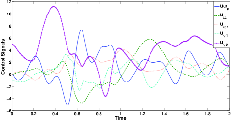
The uncertainty parameters $\theta_{0}$, $\theta_{I}$ and $\theta_{u}$ are assumed to have a uniform distribution in the interval $[1-E,1+E]$ with $E=0.2$. We select 5 values for each uncertainty parameter to construct an augmented system. We assume that the five controls $u_{m}(t)$ ($m=1,2,3,4,5$) are permitted in the Hamiltonian $H(t)$. The initial state is chosen to be the ground state $|\psi^{A}(0)\rangle=|g_{1},g_{2}\rangle$ and the target state is chosen to be $|\psi\rangle=\frac{1}{\sqrt{2}}(|e_{1},g_{2}\rangle+|g_{1},e_{2}\rangle)$. The algorithm converges with around 8000 iterations. In the evaluation step, we select 500 additional samples to test the control performance. The average fidelity we can achieve is 0.9966 and the average concurrence is 0.9880. Fig. 9 gives the learned control strategy $u_{m}(t)$ ($m=1,2,3,4,5$).

Figure 9: The learned control strategy, where the initial state is $|\psi^{A}(0)\rangle=|g_{1},g_{2}\rangle$ and the target state $|\psi^{A}_{\text{target}}\rangle=\frac{1}{\sqrt{2}}(|e_{1},g_{2}\rangle+|g_{1},e_{2}\rangle)$. The uncertainty bound is $E=0.2$, $u_{1}(t)=u{\omega_{a}}$, $u_{2}(t)=u_{\omega r}$, $u_{3}(t)=u_{\Omega}$, $u_{4}(t)=u_{\nu 1}$ and $u_{5}(t)=u_{\nu 2}$.

VII Conclusion

In this paper, we presented a systematic numerical methodology for robust control design of quantum systems. The proposed sampling-based learning control (SLC) method includes two steps of “training” and “testing”. In the training step, the control is learned using a gradient flow based learning algorithm for an augmented system constructed from samples. The learned control is evaluated for additional samples in the testing step. The proposed numerical method has been applied to three significant examples of quantum robust control including state preparation in a three-level system, entanglement generation in a superconducting quantum circuit and in a two-atom system interacting with a quantized field in a cavity. In these examples, we considered the uncertainty parameters to have uniform distributions, truncated Gaussian distributions or possibly time-varying distributions. However, numerical results showed that the uniform distribution is a sound choice for sampling the uncertainty parameters in the training step. Before we start the training step, we may first analyze the controllability of the nominal system (e.g., using Lie group and Lie algebra theory [1], [56]). Such an analysis may be difficult when we consider the constraints on control strengths and control durations. Even if we prove that the nominal system is not controllable, it may still be possible to achieve accurate state transfer between specific states that correspond to some useful practical applications. One advantage of the proposed method is that it is numerically tractable in achieving convergence since we can use a small number of samples (e.g., five or seven) for each uncertainty parameter in the training step to obtain excellent performance. Based on the training performance (whether the cost $J$ is close to one), it is easy to verify when an optimal solution has been found. The results in this paper have demonstrated the effectiveness of the SLC method for control design of quantum systems even when the uncertainty parameters have quite large fluctuations.

References

- [1] D. Dong and I.R. Petersen, “Quantum control theory and applications: A survey,” IET Control Theory & Applications, Vol.4, pp.2651-2671, 2010.
- [2] C. Altafini and F. Ticozzi, “Modeling and control of quantum systems: an introduction,” IEEE Transactions on Automatic Control, Vol.57, No.8, pp.1898-1917, 2012.
- [3] H.M. Wiseman and G.J. Milburn, Quantum Measurement and Control, Cambridge, England: Cambridge University Press, 2010.
- [4] C. Brif, R. Chakrabarti and H. Rabitz, “Control of quantum phenomena: past, present and future,” New Journal of Physics, Vol.12, p.075008, 2010.
- [5] M.A. Pravia, N. Boulant, J. Emerson, E.M. Fortunato, T.F. Havel, D.G. Cory and A. Farid, “Robust control of quantum information,” Journal of Chemical Physics, Vol.119, pp.9993-10001, 2003.
- [6] B. Qi, “A two-step strategy for stabilizing control of quantum systems with uncertainties,” Automatica, Vol.49, pp.834-839, 2013.
- [7] D. Dong, I.R. Petersen and H. Rabitz, “Sampled-data design for robust control of a single qubit”, IEEE Transactions on Automatic Control, Vol.58, pp.2654-2659, 2013.
- [8] M.R. James, “Risk-sensitive optimal control of quantum systems”, Physical Review A, Vol.69, p.032108, 2004.
- [9] N. Khaneja, T. Reiss, C. Kehlet, T. Schulte-Herbrüggen and S. J. Glaser, “Optimal control of coupled spin dynamics: desing of NMR pulse sequences by gradient ascent algorithms”, Journal of Magnetic Resonance, Vol.172, pp.296-305, 2005.
- [10] J.S. Li and N. Khaneja, “Ensemble control of Bloch equations,” IEEE Transactions on Automatic Control, Vol.54, pp.528-536, 2009.
- [11] Y. Makhlin, G. Sch n and A. Shnirman, “Quantum-state engineering with Josephson-junction devices,” Reviews of Modern Physics, Vol.73, pp.357-400, 2001.
- [12] S. Montangero, T. Calarco and R. Fazio, “Robust optimal quantum gates for Josephson charge qubits,” Physical Review Letters, Vol.99, p.170501, 2007.
- [13] H. Zhang and H. Rabitz, “Robust optimal control of quantum molecular systems in the presence of disturbances and uncertainties,” Physical Review A, Vol.49, pp.2241-2254, 1994.
- [14] M.R. James, H.I. Nurdin and I.R. Petersen, “ control of linear quantum stochastic systems”, IEEE Transactions on Automatic Control, Vol.53, pp.1787-1803, 2008.
- [15] D. Dong and I.R. Petersen, “Sliding mode control of quantum systems”, New Journal of Physics, Vol.11, p.105033, 2009.
- [16] D. Dong and I.R. Petersen, “Sliding mode control of two-level quantum systems”, Automatica, Vol.48, pp.725-735, 2012.
- [17] J. Zhang, R.B. Wu, C.W. Li and T.J. Tarn, “Protecting coherence and entanglement by quantum feedback controls”, IEEE Transactions on Automatic Control, Vol.55, No.3, pp.619-633, 2010.
- [18] F. Ticozzi, A. Ferrante and M. Pavon, “Robust steering of -level quantum systems”, IEEE Transactions on Automatic Control, Vol.49, No.10, pp.1742-1745, 2004.
- [19] G. Zhang and M.R. James, “Quantum feedback networks and control: a brief survey”, Chinese Science Bulletin, Vol.57, pp.2200-2214, 2012.
- [20] J. Zhang and R.L. Kosut, “Quantum potential design for electron transmission in semiconductor nanodevices”, IEEE Transactions on Control Systems Technology, Vol. 21, pp.869-874, 2013.
- [21] C. Chen, D. Dong, J. Lam, J. Chu and T.J. Tarn, “Control design of uncertain quantum systems with fuzzy estimators,” IEEE Transactions on Fuzzy Systems, Vol.20, No.5, pp.820-831, 2012.
- [22] B. Qi, H. Pan and L. Guo, “Further results on stabilizing control of quantum system”, IEEE Transactions on Automatic Control, Vol.58, No.5, pp.1349-1354, 2013.
- [23] D. Daems, A. Ruschhaupt, D. Sugny and S. Guérin, “Robust quantum control by a single-shot shaped pulse”, Physical Review Letters, Vol.111, p.050404, 2013.
- [24] I.R. Petersen, V. Ugrinovskii and M.R. James, “Robust stability of uncertain linear quantum systems,” Philosophical Transactions of the Royal Society A, Vol.370, pp.5354-5363, 2012.
- [25] D. Dong and I.R. Petersen, “Notes on sliding mode control of two-level quantum systems”, Automatica, Vol.48, pp.3089-3097, 2012.
- [26] N. Yamamoto, and L. Bouten, “Quantum risk-sensitive estimation and robustness”, IEEE Transactions on Automatic Control, Vol.54, pp.92-107, 2009.
- [27] G.S. Vasilev, A. Kuhn and N.V. Vitanov, “Optimum pulse shapes for stimulated Raman adiabatic passage”, Physical Review A, Vol.80, p.013417, 2009.
- [28] G. Dridi, S. Guérin, V. Hakobyan, H.R. Jauslin and H. Eleuch, “Ultrafast simulated Raman parallel adiabatic passage by shaped pulses”, Physical Review A, Vol.80, p.043408, 2009.
- [29] S. Guérin, V. Hakobyan and H.R. Jauslin, “Optimal adiabatic passage by shaped pulses: Efficiency and robustness”, Physical Review A, Vol.84, p.013423, 2011.
- [30] B.T. Torosov, S. Guérin and V. Vitanov, “High-fidelity adiabatic passage by composite sequences of chirped pulses”, Physical Review Letters, Vol.106, p.233001, 2011.
- [31] U.V. Boscain, F. Chittaro, P. Mason and M. Sigalotti, “Adiabatic control of the Schrödinger equation via conical intersections of the eigenvalues, IEEE Transactions on Automatic Control, Vol.57, pp.1970-1983, 2012.
- [32] P. Owrutsky and N. Khaneja, “Control of inhomogeneous ensembles on the Bloch sphere”, Physical Review A, Vol.86, p.022315, 2012.
- [33] A. Soare, H. Ball, D. Hayes, J. Sastrawan, M.C. Jarratt, J.J. McLoughlin, Z. Zhen, T.J. Green and M.J. Biercuk, “Experimental noise filtering by quantum control”, Nature Physics, Vol.10, pp.825-829, 2014.
- [34] R. L. Kosut, M. D. Grace and C. Brif, “Robust control of quantum gates via sequential convex programming,” Physical Review A, Vol.88, p.052326, 2013.
- [35] C. Sayrin, I. Dotsenko, X. Zhou, B. Peaudecerf, T. Rybarczyk, S. Gleyzes, P. Rouchon, M. Mirrahimi, H. Amini, M. Brune, J.-M. Raimond and S. Haroche, “Real-time quantum feedback prepares and stabilizes photon number states” Nature, Vol.477, pp.73-77, 2011.
- [36] C. Altafini, “Feedback stabilization of isospectral control systems on complex flag manifolds: Application to quantum ensembles,” IEEE Transactions on Automatic Control, Vol.52, pp.2019-2028, 2007.
- [37] R. van Handel, J. K. Stockton and H. Mabuchi, “Feedback control of quantum state reduction,” IEEE Transactions on Automatic Control, Vol.50, No.6, pp.768-780, 2005.
- [38] A.C. Doherty and K. Jacobs, “Feedback control of quantum systems using continuous state estimation,” Physical Review A, Vol.60, No.4, pp.2700-2711, 1999.
- [39] H.I. Nurdin, M.R. James and I.R. Petersen, “Coherent quantum LQG control,” Automatica, Vol.45, pp.1837-1846, 2009.
- [40] M. Mirrahimi and R. van Handel, “Stabilizing feedback controls for quantum systems”, SIAM Journal on Control and Optimization, Vol.46, No.2, pp.445-467, 2007.
- [41] L. Viola, E. Knill, and S. Lloyd, “Dynamical decoupling of open quantum systems”, Physical Review Letters, Vol.82, pp.2417-2421, 1999.
- [42] K. Khodjasteh, D.A. Lidar and L. Viola, “Arbitrarily accurate dynamical control in open quantum systems”, Physical Review Letters, Vol. 104, p.090501, 2010.
- [43] M.J. Biercuk, H. Uys, A.P. VanDevender, N. Shiga, W.M. Itano and J.J. Bollinger, “Optimized dynamical decoupling in a model quantum memory”, Nature, Vol.458, pp.996-1000, 2009.
- [44] H. Rabitz, R. de Vivie-Riedle, M. Motzkus and K. Kompa, “Whither the future of controlling quantum phenomena?” Science, Vol.288, pp.824-828, 2000.
- [45] R. Chakrabarti, and H. Rabitz, “Quantum control landscapes,” International Reviews in Physical Chemistry, Vol.26, No.4, pp.671-735, 2007.
- [46] J. Zhang, L. Greenman, X. Deng, K.B. Whaley, “Robust control pulses design for electron shuttling in solid state devices,” IEEE Transactions on Control Systems Technology, Vol.22, No.6, pp.2354-2359, 2014.
- [47] C. Chen, D. Dong, R. Long, I.R. Petersen and H. Rabitz, “Sampling-based learning control of inhomogeneous quantum ensembles”, Physical Review A, Vol.89, p.023402, 2014.
- [48] D. Dong, C. Chen, R. Long, B. Qi, I.R. Petersen, “Sampling-based learning control for quantum systems with Hamiltonian uncertainties,” Proceedings of the 52th IEEE Conference on Decision and Control, pp.1924-1929, December 10-13, 2013, Firenze, Italy.
- [49] J.Q. You and F. Nori, “Atomic physics and quantum optics using superconducting circuits,” Nature, Vol.474, pp.589-597, 2011.
- [50] J. Clarke and F. K. Wilhelm, “Superconducting quantum bits,” Nature, Vol.453, pp.1031-1042, 2008.
- [51] J.Q. You and F. Nori, “Superconducting circuits and quantum information,” Physics Today, Vol.58, pp.42-47, 2005.
- [52] Z. L. Xiang, S. Ashhab, J. Q. You and F. Nori, “Hybrid quantum circuits: Superconducting circuits interacting with other quantum systems,” Reviews of Modern Physics, Vol.85, pp.623-653, 2013.
- [53] D. Dong, C. Chen, B. Qi, I.R. Petersen and F. Nori, “Robust manipulation of superconducting qubits in the presence of fluctuations”, Scientific Reports, Vol.5, p.7873, 2015.
- [54] F. Altomare, J. I. Park, K. Cicak, M. A. Sillanpää, M. S. Allman, D. Li, A. Sirois, J. A. Strong, J. D. Whittaker and R. W. Simmonds, “Tripartite interactions between two phase qubits and a resonant cavity,” Nature Physics, Vol. 6, p.777-781, 2010.
- [55] M.A. Mabrok, D. Dong, C. Chen, I.R. Petersen, “Robust entanglement control between two atoms in a cavity using sampling-based learning control,” Proceedings of the 53th IEEE Conference on Decision and Control, pp.5802-5807, December 15-17, 2014, Los Angeles, California, USA.
- [56] D. D’Alessandro, Introduction to Quantum Control and Dynamics, Chapman & Hall/CRC, 2007.
- [57] C. Kabytayev, T.J. Green, K. Khodjasteh, M.J. Biercuk, L. Viola and K.R. Brown, “Robustness of composite pulses to time-dependent control noise”, Physical Reveiw A, Vol.90, p.012316, 2014.
- [58] M.A. Nielsen and I.L. Chuang, Quantum Computation and Quantum Information, Cambridge, England: Cambridge University Press, 2000.
- [59] C. Chen, D. Dong, H.X. Li, J. Chu and T.J. Tarn, “Fidelity-based probabilistic Q-learning for control of quantum systems”, IEEE Transactions on Neural Networks and Learning Systems, Vol. 25, pp.920-933, 2014.
- [60] R. Long, G. Riviello and H. Rabitz, “The gradient flow for control of closed quantum systems”, IEEE Transactions on Automatic Control, Vol.58, pp.2665-2669, 2013.
- [61] J. Roslund and H. Rabitz, “Gradient algorithm applied to laboratory quantum control”, Physical Reveiw A, Vol.79, p.053417, 2009.
- [62] S.C. Hou, M.A. Khan, X.X. Yi, D. Dong and I.R. Petersen, “Optimal Lyapunov-based quantum control for quantum systems,” Physical Review A, Vol.86, p.022321, 2012.
- [63] R.J. Schoelkopf and S. M. Girvin, “Wiring up quantum systems,” Nature, Vol.451, pp.664-669, 2008.
- [64] I. Chiorescu, P. Bertet, K. Semba, Y. Nakamura, C. J. P. M. Harmans and J. E. Mooij, “Coherent dynamics of a flux qubit coupled to a harmonic oscillator,” Nature, Vol.431, pp.159-162, 2004.
- [65] M.A. Sillanpää, J.I. Park and R.W. Simmonds, “Coherent quantum state storage and transfer between two phase qubits via a resonant cavity,” Nature, Vol.449, pp.438-442, 2007.
- [66] T. Yamamoto, Yu. A. Pashkin, O. Astafiev, Y. Nakamura and J. S. Tsai, “Demonstration of conditional gate operation using superconducting charge qubits,” Nature, Vol.425, pp.941-944, 2003.
- [67] Yu. A. Pashkin, T. Yamamoto, O. Astafiev, Y. Nakamura, D.V. Averin and J. S. Tsai, “Quantum oscillations in two coupled charge qubits,” Nature, Vol.421, pp.823-826, 2003.
- [68] M. Steffen, M. Ansmann, R. C. Bialczak, N. Katz, E. Lucero, R. McDermott, M. Neeley, E. M. Weig, A.N. Cleland and J. M. Martinis, “Measurement of the entanglement of two superconducting qubits via state tomography,” Science, Vol.313, pp.1423-1425, 2006.
- [69] G. Wendin and V.S. Shumeiko, in Handbook of Theoretical and Computational Nanotechnology, edited by M. Rieth and W. Schommers (American Scientific Publishers, Karlsruhe, Germany, 2006), Chap. 12; arXiv:cond-mat/0508729
- [70] M. Hofheinz, H. Wang, M. Ansmann, R.C. Bialczak, E. Lucero, M. Neeley, A.D. O’Connell, D. Sank, J. Wenner, J.M. Martinis and A.N. Cleland, “Synthesizing arbitrary quantum states in a superconducting resonator,” Nature, Vol.459, pp.546-549, 2009.
- [71] W. Cui, Z.R. Xi and Y. Pan, “The entanglement dynamics of the bipartite quantum system: toward entanglement sudden death,” Journal of Physics A: Mathematical and Theoretical, Vol.42, p.025303, 2009.
- [72] M.A. Mabrok, D. Dong, I.R. Petersen and C. Chen, “Entanglement generation in uncertain quantum systems using sampling-based learning control,” Proceedings of 19th IFAC World Congress, August 24-29, 2014, Cape Town, South Africa.
- [73] D. Bouwmeester, J.-W. Pan, K. Mattle, M. Eibl, H. Weinfurter, and A. Zeilinger, “Experimental quantum teleportation,” Nature, Vol.390, pp.575-579, 1997.
- [74] W.K. Wootters, “Entanglement of formation of an arbitrary state of two qubits”, Physical Review Letters, Vol.80, pp.2245-2248, 1998.
- [75] Z. Ficek and R. Tanaś, “Entangled states and collective nonclassical effects in two-atom systems,” Physics Reports, Vol.372, pp.369-443, 2002.
- [76] J. Majer, J. M. Chow, J. M. Gambetta, J. Koch, B. R. Johnson, J. A. Schreier, L. Frunzio, D. I. Schuster, A. A. Houck, A. Wallraff, A. Blais, M. H. Devoret, S. M. Girvin, and R. J. Schoelkopf., “Coupling superconducting qubits via a cavity bus,” Nature, Vol.449, pp.443-447, 2007.
- [77] S. Filipp, M. Göppl, J. M. Fink, M. Baur, R. Bianchetti, L. Steffen, and A. Wallraff, “Multimode mediated qubit-qubit coupling and dark-state symmetries in circuit quantum electrodynamics,” Physical Review A, Vol. 83, p.063827, 2011.
- [78] D. Jaksch, J. I. Cirac, P. Zoller, S. L. Rolston, R. Côté, and M. D. Lukin, “Fast quantum gates for neutral atoms,” Physical Review Letters, Vol. 85, pp.2208-2211, 2000.