A multiscale strategy for Bayesian inference using transport maps

Abstract

In many inverse problems, model parameters cannot be precisely determined from observational data. Bayesian inference provides a mechanism for capturing the resulting parameter uncertainty, but typically at a high computational cost. This work introduces a multiscale decomposition that exploits conditional independence across scales, when present in certain classes of inverse problems, to decouple Bayesian inference into two stages: (1) a computationally tractable coarse-scale inference problem; and (2) a mapping of the low-dimensional coarse-scale posterior distribution into the original high-dimensional parameter space. This decomposition relies on a characterization of the non-Gaussian joint distribution of coarse- and fine-scale quantities via optimal transport maps. We demonstrate our approach on a sequence of inverse problems arising in subsurface flow, using the multiscale finite element method to discretize the steady state pressure equation. We compare the multiscale strategy with full-dimensional Markov chain Monte Carlo on a problem of moderate dimension (100 parameters) and then use it to infer a conductivity field described by over 10 000 parameters.

1 Introduction

Mathematical models often contain parameters that must be estimated from observational data, before the models can be used for prediction or design. Deterministic approaches have long been applied to such inverse problems (e.g., [14, 65, 4, 20, 10]). Yet observations can seldom constrain model parameters precisely, and the resulting inverse problems are thus ill-posed. In this context, statistical approaches—e.g., the Bayesian approach [61, 38, 58]—provide a rigorous framework for simultaneously characterizing model parameters and their uncertainties [6]. This characterization is particularly crucial for applications requiring quantified uncertainties in model predictions (e.g., [67, 22, 19, 62]).

Ill-posed inverse problems often result from the combination of high-dimensional parameters and indirect observations, especially when the observations smooth or integrate the parameter field of interest. In this setting, the map from parameters to observations is called the forward model. Smoothing forward models are ubiquitous in science and engineering applications, ranging from flow through porous media to tomography and remote sensing. A significant body of research has sought to develop and analyze multiscale methods for evaluating such forward models [29, 31, 3, 26, 17, 35, 36, 1, 37]. Many of these methods rely on the idea that a finite dimensional coarse-scale representation can include the impact of fine-scale structure in the parameters without resolving the problem to that level. For example, in the context of partial differential equations (PDEs), fine-scale spatial variation in a coefficient or initial condition can be captured by homogenized coefficients, coarse-scale basis functions, or other correction terms to the variational statement of the problem, enabling the PDE solution to be accurately approximated at reduced cost. A host of theoretical developments and numerical approaches [30, 53, 32] have yielded multiscale solution strategies for linear and nonlinear PDEs, ODEs, and other systems [45].

Implicit in the success of a multiscale strategy for solving the forward model is a notion of conditional independence: observations of the solution can be directly predicted by some coarse-scale quantities; conditioned on these coarse-scale quantities, the observations and the original parameter field of interest (which resolves fine-scale structure) are independent. We will use this notion to design a multiscale Bayesian inference approach. Our approach will decompose the inverse problem into a coarse-scale inference problem, where coarse-scale quantities are inferred from data, and a fine-scale inference problem, where fine-scale parameters are conditioned on realizations of the coarse scale. This strategy will reduce the effective parameter dimension of the inverse problem, increase parameter identifiability, and provide significant opportunities for parallel computation. Our framework will accommodate nonlinear, non-deterministic, and non-Gaussian relationships between the coarse- and fine-scale quantities. The specific coarse-scale quantity that we employ is entirely flexible in that it is a consequence of the multiscale solution method chosen for the forward problem; our framework is thus, in principle, applicable to a variety of multiscale modeling methods and a broad array of problems containing multiscale structure.

In the Bayesian setting, knowledge about the values and structure of the parameters is represented via the assignment of probabilities [33, 34, 61, 38, 58, 23]. The prior probability distribution represents an initial state of knowledge, which is updated via the likelihood function to obtain the posterior distribution. The likelihood often couples a physics-based forward model (e.g., a PDE) with a probabilistic description of observation and model errors. Except in simple cases, the posterior distribution cannot be characterized in closed form and one must instead resort to sampling approaches, e.g., Markov chain Monte Carlo (MCMC) [54, 9, 41], importance sampling [41], sequential Monte Carlo [16], or variational approaches including transport maps [47]. High-dimensional parameter spaces and computationally expensive models make all of these methods more challenging to apply. Significant research effort has thus been devoted to dimension reduction approaches that can make sampling more efficient, and reduce the number of forward model evaluations required.

For example, in the Bayesian approach to inverse problems, Karhunen-Loève (KL) expansions based on the prior [40, 18, 43] have proven useful in reducing parameter dimension. But this approach is practically limited to rather smoothing priors, and does not account for the forward model and the data in identifying relevant parameter directions. More recent work has introduced the notion of a likelihood-informed subspace (LIS), which contains parameter directions where the posterior distribution is most different from the prior [13, 56, 12]. Construction of the LIS requires finding the dominant eigenmodes of the Hessian of the log-likelihood, preconditioned by the prior covariance, at many points in the parameter space. These approaches rely on a heuristic globalization of Hessian information, but yield only a linear subspace of the original parameter space.

Other approaches to dimension reduction in Bayesian inversion explicitly take advantage of multiscale structure. Existing approaches generally do so in two ways: (1) by using multiple discretizations of the parameter field itself [27, 28, 68], or (2) by employing efficient multiscale numerical solvers for the forward model. [18] and [15] are in this second category and are most related to the present work. These efforts perform inference on a single discretization of the parameter field, but use a multiscale forward solver to drive a “delayed-acceptance” MCMC scheme [11], where proposed samples are first accepted or rejected according to an approximation of the forward model solution. These approaches improve MCMC efficiency but still require, per accepted sample, at least one new forward solve that explicitly resolves the fine scales. [48, 49] analyze the impact of the homogenization of elliptic operators on parameter estimates. This analysis requires specific forms for the parameter fields, however, and focuses on maximum a posteriori (MAP) estimation rather than the full Bayesian posterior.

With the exception of [48] and [49], the multiscale sampling approaches described above seek to accelerate asymptotically exact sampling of a posterior distribution on a fine-scale representation of the parameters. Repeated calls to a forward solver that resolves the fine scales then remain an “online” part of each inference algorithm—in the sense that these calls must be performed after observations are obtained. This requirement carries significant computational expense. We will exploit multiscale structure in a different manner, approximating the posterior according to the conditional independence assumptions described earlier and reducing the online time required for posterior exploration. We generate a posterior on the coarse-scale representation and use the conditional distribution of the fine scales to “prolong” samples of the coarse-scale posterior to the original high-dimensional parameter space containing fine-scale structure. In contrast with many previous approaches, we do not require particular forms for the forward model or prior distribution; we avoid globally resolving the fine scales in any forward solves; and we allow for rather general multiscale models whose coarse or fine features may not even lie on a mesh.

To capture the stochastic and in general non-Gaussian relationship among the scales, we will rely on transport maps—deterministic functions that push forward a reference distribution to a more complex target distribution. We will construct transport maps in a particular form that enables efficient marginalization and conditioning, both of which are basic operations for our multiscale inference framework. Importantly, these transport maps can be constructed a priori, before any data is observed, significantly reducing online computational effort. We will also take advantage of stationarity and locality, when present in the problem, to accelerate the construction of transport maps that represent the joint distribution of the fine and coarse scales.

The remainder of this paper is organized as follows. Section 2 introduces a multiscale decomposition of the inverse problem in a Bayesian setting. Section 3 introduces transport maps and shows how they can be used to render the decomposition of Section 2 into an effective algorithm. Section 4 provides a small illustrative example, Section 5 describes strategies for applying the multiscale framework to elliptic PDE inverse problems, and Section 6 demonstrates the efficiency of our approach on two large subsurface flow applications.

2 A framework for multiscale Bayesian inference

Let $\theta$ be a random variable taking values in ${}^{d_{\theta}}$. In the discussion below, $\theta$ will represent the parameter field we wish to infer, which may contain fine scale structure. For simplicity, we will assume that all probability distributions have densities with respect to Lebesgue measure. To keep notation straightforward, we will also specify density functions by their arguments, except where this might be ambiguous.

In the Bayesian context, the prior probability density $\pi(\theta)$ represents prior knowledge about the random variable $\theta$. Observations are represented by an ${}^{d_{y}}$-valued random variable $y$; conditioning on a particular value of these observations then yields a posterior probability density according to Bayes’ rule:

(1) $$\pi(\theta|y)=\frac{\pi(y,\theta)}{\pi(y)}=\frac{\pi(y|\theta)\pi(\theta)}{\pi(y)}\propto\pi(y|\theta)\pi(\theta).$$

Here $\pi(y|\theta)$, viewed as a function of $\theta$, is the likelihood function. The normalizing constant $\pi(y)$ is called the evidence. In the Bayesian setting for inverse problems, the likelihood function typically contains a deterministic forward model $f$, and compares $f(\theta)$ to $y$ according to a statistical model for observation and model errors [38, 58].

2.1 A statistical definition for multiscale models

Many systems contain parameterized features or dynamics that span multiple scales of spatial or temporal variation. Of course, this is a rather general observation. To be more precise, our framework employs a specific definition of “multiscale” structure. We will say that a model mapping $\theta$ to $y$ has multiscale structure if there is a quantity $\gamma$ such that $y$ and $\theta$ are conditionally independent given $\gamma$, i.e.:

(2) $$\pi(y|\gamma,\theta)=\pi(y|\gamma).$$

Very often $\gamma$ will be naturally suggested by the forward model, and will represent a coarse-scale quantity derived from the parameters $\theta$ and the forward operator. To make the introduction of the coarse-scale quantity useful, the dimension of $\gamma$, denoted by $d_{\gamma}$, should be smaller than the dimension of $\theta$.

Even though this definition might seem abstract, many real systems exhibit behavior that approximately satisfies (2). For example, any deterministic model $f(\theta)$ that can be written as $f(\theta)=\tilde{f}\left(g(x)\right)$, where $\tilde{f}:^{d_{\gamma}}\rightarrow^{d_{y}}$ and $g:^{d_{\theta}}\rightarrow^{d_{\gamma}}$, will yield a posterior that satisfies (2). In subsurface flow applications, for instance, $\theta$ could be a conductivity field discretized on a mesh that resolves the fine scales and $\gamma=g(\theta)$ could be a coarse “upscaled” conductivity field, where $f$ and $\tilde{f}$ provide predictions of hydraulic head. Further examples exist in any application where observables depend on some aggregate, integrated, or homogenized behavior of the fine scale parameter $\theta$.

Of course, in many systems, the equality (2) is only approximately satisfied. With the resulting likelihood approximation $\pi(y|\gamma,\theta)\approx\pi(y|\gamma)$, only approximate posterior samples of $\theta$ can be obtained. In applications where multiscale forward modeling has been successful, however, this approximation error can be quite small. Moreover, in practice, the computational advantages of using the coarse parameter $\gamma$ may greatly outweigh the drawbacks of a posterior approximation. As we will demonstrate in Section 6.2, exploiting multiscale structure can allow us to tackle very large problems where directly sampling $\pi(\theta|y)$ is otherwise intractable.

2.2 Algorithmic building blocks: decoupling the coarse and fine scales

In the usual “single-scale” setting, we obtain a posterior $\pi(\theta|y)$ according to Bayes’ rule as shown in (1). Let us instead consider the joint posterior distribution of the coarse- and fine-scale parameters $(\theta,\gamma)$:

$$\pi(\theta,\gamma|y) \propto \pi(y|\theta,\gamma)\pi(\gamma,\theta)$$

$$\approx \pi(y|\gamma)\pi(\gamma,\theta)$$

$$= \pi(y|\gamma)\pi(\gamma)\pi(\theta|\gamma)\,.$$

In moving from the first line to the second, we applied the conditional independence assumption (2). Then we expanded the joint prior $\pi(\gamma,\theta)$ into the marginal prior of the coarse quantity $\gamma$ and the conditional prior distribution of the fine scales given the coarse. This resulting expression is the foundation of our multiscale inference framework. The three densities on the right hand side of (2.2) can be understood as a coarse likelihood, a coarse prior, and a downscaling “prolongation” density. Notice that only the downscaling density involves the high-dimensional fine scale parameters $\theta$.

It is trivial to remove $\theta$ from (2.2) via marginalization, leaving the posterior density of the coarse parameters alone: $\pi(\gamma|y)\propto\pi(y|\gamma)\pi(\gamma)$. We can now break sampling the fine-scale posterior $\pi(\theta|y)$ into two steps: (1) coarse-scale inference, which samples the posterior $\pi(\gamma|y)$ directly and ignores the fine scale parameters; and (2) fine-scale conditioning, which generates one or more samples of the fine-scale parameter from $\pi(\theta|\gamma^{(i)})$, for each posterior sample $\gamma^{(i)}$. Since $\pi(\theta|y,\gamma)=\pi(\theta|\gamma)$ under the conditional independence assumption, the combination of these two steps will generate samples from the joint posterior $\pi(\theta,\gamma|y)=\pi(\theta|\gamma,y)\pi(\gamma|y)$. Marginalizing out the coarse parameter (i.e., simply ignoring the coarse component of each joint sample) will produce samples of the fine-scale posterior $\pi(\theta|y)=\int\pi(\theta,\gamma|y)d\gamma$.

While this two-step process is conceptually simple, two important issues remain:

1. Sampling the coarse-scale posterior in principle requires evaluating the prior density $\pi(\gamma)$ of the coarse parameter $\gamma$. But the original inference problem only specifies a prior on the fine-scale parameter $\theta$.

2. Generating fine-scale posterior samples requires that we sample from the conditional density $\pi(\theta|\gamma)$; in general cases, this task may be nontrivial.

Both of these issues will be addressed through the construction of transport maps that represent the joint prior distribution of the coarse- and fine-scale quantities, with a particular structure described in the next section.

3 Transport maps for multiscale inference

Transport maps are deterministic nonlinear variable transformations between (probability) measures [63, 64]. Transport maps have recently been used to accelerate Bayesian inference, coupled with MCMC [52] or in a standalone approach [47]. Compositions of many simple transport maps have also been used for density estimation in [60, 59]. Here we will use transport maps to transform the joint prior density $\pi(\gamma,\theta)$ into a standard normal distribution that can be easily sampled. Constructing this transformation with the appropriate structure will enable easy characterization of the coarse prior density $\pi(\gamma)$ and sampling from downscaling density $\pi(\theta|\gamma)$.

3.1 Transport maps

To define a transport map, consider two Borel probability measures on ^d, denoted by $\mu$ and $\nu$. We will call these the target and reference measures, respectively, and associate them with random variables $x\sim\mu$ and $r\sim\nu$. An exact transport map $T:^{d}\rightarrow^{d}$ is a deterministic transformation that pushes forward $\mu$ to $\nu$, yielding

(4) $$\nu(A)=\mu\left(T^{-1}(A)\right)$$

for any Borel measurable set $A\subseteq^{d}$. This pushforward relationship is denoted concisely by $\nu=T_{\sharp}\mu$. In terms of the random variables, we may write $r\buildrel i.d.\over{=}T(x)$, where $\buildrel i.d.\over{=}$ denotes equality in distribution.

Existence of a $T$ satisfying (4) is guaranteed when $\mu$ has no atoms [8, 44], but there can be infinitely many transport maps between two arbitrary probability measures. To regularize the problem, and for additional reasons described below, we restrict our attention to maps with the following lower triangular structure:

(5) $$T(x_{1},x_{2},\ldots,x_{d})=\left[\begin{array}[]{l}T_{1}(x_{1})\\ T_{2}(x_{1},x_{2})\\ \vdots\\ T_{d}(x_{1},x_{2},\ldots,x_{d})\end{array}\right],$$

where subscripts denote components of $x\in^{d}$. This lower triangular map is known as the Knothe-Rosenblatt (K-R) rearrangement. For absolutely continuous target and reference measures, the K-R map exists and is uniquely defined (up to ordering of the coordinates), and has a lower triangular Jacobian with positive diagonal entries ($\mu$-a.e.). The map is thus a bijection between the ranges of $x$ and $r$. This lower triangular structure will be particularly useful for our multiscale approach, as we explain in the next section.

3.2 Exact multiscale inference

Let the reference random variable be composed of independent standard Gaussians, $r\sim N(0,I)$, and let the target measure be the joint prior on $x:=(\gamma,\theta)$. In this section, we suppose that we have a lower triangular map $T:^{d_{\gamma}+d_{\theta}}\rightarrow^{d_{\gamma}+d_{\theta}}$ that pushes forward the prior to the reference, i.e.,

(6) $$r=\left[\begin{array}[]{c}r_{c}\\ r_{f}\end{array}\right]\buildrel i.d.\over{=}\left[\begin{array}[]{l}T_{c}(\gamma)\\ T_{f}(\gamma,\theta)\end{array}\right]=T(\gamma,\theta),$$

where $r_{c}$ and $r_{f}$ are standard Gaussian random variables with dimensions $d_{\gamma}$ and $d_{\theta}$, respectively. In Section 3.3 we will discuss how to construct such a map, but for now we proceed as if we have an exact transport map in hand. It will be convenient to define $S:^{d_{\gamma}+d_{\theta}}\rightarrow^{d_{\gamma}+d_{\theta}}$ as the lower triangular inverse of $T(\gamma,\theta)$, such that

(7) $$S(r)=\left[\begin{array}[]{l}S_{c}(r_{c})\\ S_{f}(r_{c},r_{f})\end{array}\right]\buildrel i.d.\over{=}\left[\begin{array}[]{l}\gamma\\ \theta\end{array}\right].$$

We now wish to use the upper block of (7) to rewrite the prior and posterior on the coarse-scale quantity $\gamma$. Effectively we will “transfer” the coarse-scale inference problem to the reference variable $r_{c}$ via the bijection $T_{c}=S_{c}^{-1}$. The pullback of the prior marginal $\pi_{\gamma}(\gamma)$ through $S_{c}$ has the following density:

$$\pi_{\gamma}\left(S_{c}(r_{c})\right)|\det\nabla S_{c}(r_{c})|=p(r_{c}),$$

where $p$ denotes the standard normal density. Thus, knowing the transport map $S_{c}$ enables us to evaluate the coarse-scale prior density $\pi_{\gamma}$. But we can go one step further, applying the same variable transformation to the coarse posterior $\pi_{\gamma|y}(\gamma|y)\propto\pi_{y|\gamma}(y|\gamma)\pi_{\gamma}(\gamma)$ in order to obtain a posterior on $r_{c}$:

$$\pi(r_{c}|y) = \pi_{\gamma|y}\left(S_{c}(r_{c})|y\right)|\det\nabla S_{c}(r_{c})|$$

$$\propto \pi_{y|\gamma}\left(y|S_{c}(r_{c})\right)\pi_{\gamma}\left(S_{c}(r_{c})\right)|\det\nabla S_{c}(r_{c})|$$

$$= \pi_{y|\gamma}\left(y|S_{c}(r_{c})\right)p(r_{c})$$

$$= \pi(y|r_{c})\,p(r_{c}).$$

Parameterizing the coarse-scale inference problem in terms of $r_{c}$ is convenient as now the prior is simply standard normal.

Next, we can use the maps (6) and (7) to generate samples from the fine-scale conditional density $\pi(\theta|\gamma)$. Since $T_{c}$ is a bijection, sampling from $\pi(\theta|\gamma^{\ast})$ for a fixed value $\gamma^{\ast}$ is equivalent to sampling $\pi(\theta|r_{c}^{\ast})$ when $T_{c}(\gamma^{\ast})=r_{c}^{\ast}$. With the help of $S_{f}$, we can simulate the random variable $\theta|r_{c}^{\ast}$ whose density is $\pi(\theta|r_{c}^{\ast})$ using the fact that

(9) $$\theta|r_{c}^{\ast}\buildrel i.d.\over{=}S_{f}(r_{c}^{\ast},r_{f}).$$

According to this expression, samples of $\theta|r_{c}^{\ast}$ can be generated by first sampling the standard Gaussian $r_{f}$ and then evaluating the map $S_{f}$.

We combine these coarse- and fine-scale sampling strategies to define our complete multiscale framework. The conditional independence property (2) and the maps $S$ and $T$ allow us to sample the fine-scale posterior $\theta|y$ in two steps:

1. Use MCMC or any other standard sampling strategy to sample the coarse posterior $\pi(r_{c}|y)$ defined in (3.2).

2. For each coarse posterior sample $r_{c}^{\ast}$, generate one or more samples of $r_{f}$ from a standard normal distribution and evaluate $S_{f}(r_{c}^{\ast},r_{f})$ to obtain fine-scale posterior samples.

This procedure is detailed on lines 10–14 of Algorithm 1. Clearly, the maps $T$ and $S$ are critical to our approach. Next we will discuss how to construct these transformations.

3.3 Constructing transport maps from samples

Our construction of the “forward” (reference to target) map $S$ will depend on the “inverse” (target to reference) map $T$, so we will first focus on the construction of $T$. Consider the pullback of the standard normal reference measure through a candidate map $T$; this pullback distribution has density $\tilde{\pi}(\gamma,\theta)$:

(10) $$\tilde{\pi}(\gamma,\theta)=p\left(T(\gamma,\theta)\right)\left|\det{\nabla T}(\gamma,\theta)\right|,$$

where ${\nabla T}$ is the Jacobian of $T$ and $\det{\nabla T}$ is the determinant of the Jacobian. To simplify notation, we again let $x=(\gamma,\theta)$, so that the target density is $\pi(\gamma,\theta)=\pi(x)$.

We evaluate the difference between the target density $\pi$ and map-induced density $\tilde{\pi}$ using the Kullback-Leibler (KL) divergence:

$$D_{\text{KL}}(\pi\|\tilde{\pi}) = \mathbb{E}_{\pi}\left[\log{\left(\frac{\pi(x)}{\tilde{\pi}(x)}\right)}\right]$$

$$= \mathbb{E}_{\pi}\left[\log{\left(\frac{\pi(x)}{p\left(T(x)\right)\left|\det{\nabla T}(x)\right|}\right)}\right]$$

$$= \mathbb{E}_{\pi}\left[\log{\pi(x)}-\log{p\left(T(x)\right)}-\log{\left|\det{\nabla T}(x)\right|}\right],$$

where $\mathbb{E}_{\pi}$ denotes the expectation with respect to the joint prior density $\pi(x)$. Using (3.3), we will find transport maps by solving the minimization problem

(12) $$\min_{T\in{\mathcal{T}}}\mathbb{E}_{\pi}\left[-\log{p\left(T(x)\right)}-\log{\left|\det{\nabla T}(x)\right|}\right].$$

Note that $\log{\pi(x)}$ was removed from the objective because it does not depend on $T$. ${\mathcal{T}}$ is the space of monotone, continuously differentiable, and lower triangular maps from ${}^{d_{\gamma}+d_{\theta}}$ to ${}^{d_{\gamma}+d_{\theta}}$. For a sufficiently smooth joint density $\pi(x)$, ${\mathcal{T}}$ will contain the Knothe-Rosenblatt map and hence the solution to (12) will be an exact measure transformation, for which $D_{\text{KL}}(\pi\|\tilde{\pi})=0$.

In most situations, the minimization problem (12) must be approximated in two respects: first, because the expectation cannot be computed exactly, and second, because the map might be represented in a space ${\widetilde{\mathcal{T}}}\subset{\mathcal{T}}$ that does not include the exact Knothe-Rosenblatt map. In these situations, we instead find an approximate lower triangular map ${\widetilde{T}}$ such that ${\widetilde{T}}(x)\buildrel i.d.\over{\approx}r$. Suppose we have $K$ samples $x^{(k)}$ from the joint prior $\pi(x)$. We can use these samples to define a Monte Carlo approximation of the expectation in (12). As detailed in [52], one can define the approximate map ${\widetilde{T}}$ as the solution of the minimization problem

(13) $$\underset{{\widetilde{T}}\in{\widetilde{\mathcal{T}}}}{\min} -\frac{1}{K}\sum_{k=1}^{K}\left[\log{p\left({\widetilde{T}}(x^{(k)})\right)}+\sum_{i=1}^{d_{\gamma}+d_{\theta}}\log{\frac{\partial{\widetilde{T}}(x^{(k)})}{\partial x_{i}}}\right],$$

s.t. $$\frac{\partial{\widetilde{T}}_{i}(x^{(k)})}{\partial x_{i}}\geq\lambda_{\text{min}}>0,\quad k\in\{1,2,\ldots,K\},\quad i\in\{1,2,\ldots,d_{\gamma}+d_{\theta}\},$$

where $\lambda_{\text{min}}$ is a small positive scalar introduced to ensure monotonicity and ${\widetilde{\mathcal{T}}}$ is the space of maps spanned by a finite set of basis functions $\{\psi_{1},\psi_{2},\ldots,\psi_{N}\}$. Note that the log-determinant term has been expanded into a sum and that the absolute value has been removed; this is a result of using a monotonically increasing lower triangular map. In this work, we use multivariate Hermite polynomials to represent the map. These polynomial basis functions will also be combined with problem-specific structure (discussed in Section 5) to facilitate map construction in high dimensions.

While [52] solved (14) directly (though in a different context, with samples generated via MCMC), the applications in this paper are of much higher dimension. We have found that additional constraints on ${\widetilde{T}}$ can help obtain accurate maps with fewer samples. Using the fact that the reference density $p(r)$ is a standard normal, we constrain the output of ${\widetilde{T}}$ to have unit sample variance and zero sample mean. With these constraints, the optimization problem for ${\widetilde{T}}_{i}$ becomes

(14) $$\underset{{\widetilde{T}}\in{\widetilde{\mathcal{T}}}_{i}}{\min} -\frac{1}{K}\sum_{k=1}^{K}\left[\sum_{i=1}^{d_{\gamma}+d_{\theta}}\log{\frac{\partial{\widetilde{T}}_{i}(x^{(k)})}{\partial x_{i}}}\right]$$

s.t. $$\frac{\partial{\widetilde{T}}_{i}(x^{(k)})}{\partial x_{i}}\geq\lambda_{\text{min}}>0,\quad k\in\{1,2,\ldots,K\},\quad i\in\{1,2,\ldots,d_{\gamma}+d_{\theta}\}$$

$$\frac{1}{K}\sum_{k=1}^{K}{\widetilde{T}}_{i}(x^{(k)})=0,\quad i\in\{1,2,\ldots,d_{\gamma}+d_{\theta}\}$$

$$\frac{1}{K}\sum_{k=1}^{K}{\widetilde{T}}_{i}^{2}(x^{(k)})=1,\quad i\in\{1,2,\ldots,d_{\gamma}+d_{\theta}\}.$$

Notice that we have removed the $\log{p\left({\widetilde{T}}(x^{(k)})\right)}$ term from the objective. Because the reference density $p(\cdot)$ is standard normal, $\sum_{k=1}^{K}\log{p\left({\widetilde{T}}(x^{(k)})\right)}\propto-\sum_{k=1}^{K}{\widetilde{T}}^{2}(x^{(k)})$; hence, satisfying the variance constraint ensures that this term is constant. The additional constraints in (14) make it slightly more difficult to solve than (13), but in our experience, imposing the mean and variance information yields more accurate maps, warranting the extra effort required during optimization. We should note that (14) is non-convex because of the quadratic constraint. However, we have not found this property to cause convergence issues in practice; future work might be able to explain this fact by extending the global minimum ideas from [46].

The structure of the constrained optimization problem (14) also enables several efficient solution approaches. First, when the map parameterization is independent across each dimension (e.g., each component of the map is represented with its own expansion), the optimization problem in (14) is separable. Thus we can independently solve $d_{\gamma}+d_{\theta}$ smaller optimization problems instead of one large optimization problem. Next, we will ensure that each ${\widetilde{T}}_{i}$ is linear in the coefficients of its basis representation (e.g., a polynomial expansion); as a result, the objective can be evaluated using efficient linear algebra routines.

Let each component ${\widetilde{T}}_{i}$ of the map be expressed in the form

(15) $${\widetilde{T}}_{i}(x)=\sum_{\mathbf{j}\in\mathcal{J}_{i}}\alpha_{i,\mathbf{j}}\psi_{\mathbf{j}}(x),$$

where $\alpha_{i,\mathbf{j}}$ is the coefficient for the basis function $\psi_{\mathbf{j}}(x)$, $\psi_{\mathbf{j}}(x)$ is a multivariate Hermite polynomial whose degrees in each coordinate are specified by the multi-index $\mathbf{j}$, and the multi-index set $\mathcal{J}_{i}$ defines the basis functions used for output dimension $i$ of the map. Note that the triangular structure of the map can be encoded through the choices of $\mathcal{J}_{i}$. With this representation, optimization over ${\widetilde{T}}$ is equivalent to optimizing over the map coefficients. Using (15), we now define two Vandermonde matrices $A_{i}$ and $G_{i}$ containing evaluations of the basis functions and their derivatives, respectively. Let $\mathcal{J}_{i}=\{j_{i,1},j_{i,2},\ldots,j_{i,|\mathcal{J}_{i}|}\}$, where $|\mathcal{J}_{i}|$ is the cardinality of $\mathcal{J}_{i}$. Then these matrices take the form

(16) $$A_{i}=\left[\begin{array}[]{cccc}\psi_{j_{i,1}}(x^{(1)})&\psi_{j_{i,2}}(x^{(1)})&\ldots&\psi_{j_{i,|\mathcal{J}_{i}|}}(x^{(1)})\\ \psi_{j_{i,1}}(x^{(2)})&\psi_{j_{i,2}}(x^{(2)})&\ldots&\psi_{j_{i,|\mathcal{J}_{i}|}}(x^{(2)})\\ \vdots&\vdots&&\vdots\\ \psi_{j_{i,1}}(x^{(K)})&\psi_{j_{i,2}}(x^{(K)})&\ldots&\psi_{j_{i,|\mathcal{J}_{i}|}}(x^{(K)})\end{array}\right],$$

and

(17) $$G_{i}=\left[\begin{array}[]{cccc}\frac{\partial\psi_{j_{i,1}}}{\partial x_{i}}(x^{(1)})&\frac{\partial\psi_{j_{i,2}}}{\partial x_{i}}(\gamma^{(1)})&\ldots&\frac{\partial\psi_{j_{i,|\mathcal{J}_{i}|}}}{\partial x_{i}}(x^{(1)})\\ \frac{\partial\psi_{j_{i,1}}}{\partial x_{i}}(x^{(2)})&\frac{\partial\psi_{j_{i,2}}}{\partial x_{i}}(x^{(2)})&\ldots&\frac{\partial\psi_{j_{i,|\mathcal{J}_{i}|}}}{\partial x_{i}}(x^{(2)})\\ \vdots&\vdots&&\vdots\\ \frac{\partial\psi_{j_{i,1}}}{\partial x_{i}}(x^{(K)})&\frac{\partial\psi_{j_{i,2}}}{\partial x_{i}}(x^{(K)})&\ldots&\frac{\partial\psi_{j_{i,|\mathcal{J}_{i}|}}}{\partial x_{i}}(x^{(K)})\end{array}\right].$$

With these matrices in hand, the optimization problem from (14) can be written simply as

(18) $$\underset{\alpha_{i}}{\min} -c^{\top}\log{\left(G_{i}\alpha_{i}\right)}$$

s.t. $$G_{i}\alpha_{i} \geq\lambda_{\text{min}},$$

$$c^{\top}A_{i}\alpha_{i} =0,$$

$$\alpha_{i}^{\top}A_{i}^{\top}A_{i}\alpha_{i} =K,$$

for each $i\in\{1,\ldots,d_{\gamma}+d_{\theta}\}$, where the $\log$ is taken componentwise, $c$ is a length-$K$ vector of ones, and $\alpha_{i}$ is a vector of the expansion coefficients. This problem can now be solved easily using any technique for constrained optimization. In particular, we use an augmented Lagrangian method [2, 39] to handle the constraints and a full Newton optimizer with backtracking line search on the unconstrained subproblems. More advanced methods or implementations like IPOPT [66] or ADMM [7] might reduce the computational effort needed to solve the optimization problem in (18). In our experience, however, the main computational cost of map construction does not lie in solving (18), but rather in generating the $K$ prior samples of $x=(\gamma,\theta)$ needed to define (16) and (17).

3.4 From inverse map to forward map

Recall that the posterior sampling procedure in Section 3.2 requires evaluations of the maps $S_{c}$ and $S_{f}$ in (7), which push forward the standard normal reference distribution to the joint prior distribution $\pi(x)$. As proposed in [52], taking advantage of the lower triangular structure, it is possible to evaluate the inverse of $T$ (that is, $S$) using a sequence of one-dimensional polynomial solves. However, when many evaluations of $\widetilde{S}$ are required, it is more efficient to approximate $S$ directly and to evaluate this approximation without explicitly inverting $T$. We now define a regression procedure that constructs an approximation $\widetilde{S}$ of $S$, using the map ${\widetilde{T}}$ and the samples $\{x^{(k)}\}$.

Using each joint sample $x^{(k)}$, we can compute $r^{(k)}={\widetilde{T}}\left(x^{(k)}\right)$ to obtain sample pairs corresponding to the input and output of $S$. With these pairs, we can construct $S$ with standard least squares regression. The least squares objective is

(19) $$\min_{\widetilde{S}}\sum_{k=1}^{K}\left(\widetilde{S}(r^{(k)})-x^{(k)}\right)^{2}.$$

As with ${\widetilde{T}}$, we represent the triangular map $\widetilde{S}$ using an expansion of multivariate Hermite polynomials. This allows us to find the coefficients of the map that minimizes (19) using standard linear least squares techniques (i.e., the QR decomposition of a Vandermonde matrix). The convergence properties of similar regression-based maps were studied by [57] in a discrete optimal transport setting.

3.5 A complete algorithm for multiscale inference

The entire process of generating fine-scale posterior samples using our multiscale inference framework is described in Algorithm 1.

Input: A way to sample the fine-scale prior distribution $\pi(\theta)$; a way to sample the upscaling distribution $\pi(\gamma|\theta)$; the number of coarse posterior samples $N$; and the number of fine samples per coarse sample $M$.

Output: Samples of the fine scale posterior $\pi(\theta|y)$

/* Step 1: Generate prior samples */

1 for $k\leftarrow 1\textbf{ to }K$ do

2       Sample $\theta^{(k)}$ from $\pi(\theta)$

3       Sample $\gamma^{(k)}$ given $\theta^{(k)}$

/* Step 2: Compute the forward map ${\widetilde{T}}$ */

4 for $i\leftarrow 1\textbf{ to }d_{\theta}+d_{\gamma}$ do

5       Solve (18) to get ${\widetilde{T}}_{i}$

6      

/* Step 3: Generate sample pairs and solve for the inverse map $\widetilde{S}$ */

7 for $k\leftarrow 1\textbf{ to }K$ do

8       $\left(r_{c}^{(k)},r_{f}^{(k)}\right)={\widetilde{T}}\left(\gamma^{(k)},\theta^{(k)}\right)$

9      

10Solve (19) to get $\widetilde{S}_{c}$ and $\widetilde{S}_{f}$

/* Step 4: Sample the coarse posterior */

11 Generate $\left\{r_{c}^{(1)},r_{c}^{(2)},\ldots,r_{c}^{(N)}\right\}$ from $\pi(r_{c}|y)$ (3.2), using MCMC or another sampling method

/* Step 5: Generate fine scale posterior samples */

12 for $i\leftarrow 1\textbf{ to }N$ do

13       for $j\leftarrow 1\textbf{ to }M$ do

14             Sample $r_{f}^{(i,j)}$ from a standard Gaussian

15             $\theta^{(iM+j)}\leftarrow\widetilde{S}_{f}\left(r_{c}^{(i)},r_{f}^{(i,j)}\right)$

16            

17      

18return Posterior samples $\left\{\theta^{(1)},\theta^{(2)},\ldots,\theta^{(NM)}\right\}$

Algorithm 1 Overview of the entire multiscale inference framework.

3.6 Choosing the number of fine scale samples

After sampling the coarse-scale posterior (line 9 of Algorithm 1), we have a set of (possibly correlated) samples $\{r_{c}^{(1)},r_{c}^{(2)},\ldots,r_{c}^{(N)}\}$ from $\pi(r_{c}|y)$. The next step is to “prolong” these samples back to the fine scale by sampling $\pi(\theta|r_{c}^{(i)})$ for each $i$. If our goal is to minimize the computational effort required to estimate the posterior expectation of a $\theta$-dependent quantity with a certain accuracy, it is useful to consider how the variance of the estimator depends on the number of fine scale samples $M$ produced for each coarse scale sample. There is a tradeoff between reducing the coarse-scale contribution to the variance (by increasing $N$) and reducing the conditional fine-scale contribution to the variance (by increasing $M$). The optimal choice depends on the computational cost of generating each kind of sample, on the degree of correlation among the coarse-scale samples, and on the magnitudes of the variances on the coarse and fine scales.

For simplicity, suppose that we are interested in the fine-scale posterior mean $\mathbb{E}[\theta|y]$. Using $M$ fine scale samples for each of the $N$ coarse samples, a Monte Carlo estimator of $\mathbb{E}[\theta|y]$ is

(20) $$\widehat{{\theta}}(\mathbf{r_{c}},\mathbf{r_{f}})=\frac{1}{NM}\sum_{i=1}^{N}\sum_{j=1}^{M}\widetilde{S}_{f}\left(r_{c}^{(i)},r_{f}^{(i,j)}\right),$$

where $\mathbf{r_{c}}$ is a set of $N$ correlated samples of $\pi(r_{c}|y)$ and $\mathbf{r_{f}}$ is a set containing the $NM$ fine scale samples.

We wish to choose $M$ in order to minimize the variance of the estimator $\widehat{\theta}$ for a given computational effort. This variance can be expanded (using the law of total variance) as

$${\mathbb{V}\mathrm{ar}}_{\mathbf{r_{c}},\mathbf{r_{f}}}\left[\widehat{{\theta}}(\mathbf{r_{c}},\mathbf{r_{f}})\right] = {\mathbb{V}\mathrm{ar}}_{\mathbf{r_{c}}}\left[\mathbb{E}_{\mathbf{r_{f}}}\left\{\widehat{\theta}(\mathbf{r_{c}},\mathbf{r_{f}})|\mathbf{r_{c}}\right\}\right]+\mathbb{E}_{{\mathbf{r_{c}}}}\left[{\mathbb{V}\mathrm{ar}}_{\mathbf{r_{f}}}\left\{\widehat{\theta}(\mathbf{r_{c}},\mathbf{r_{f}})|\mathbf{r_{c}}\right\}\right]$$

$$= \frac{C_{1}}{N}+\frac{C_{2}}{NM},$$

where $C_{1}$ and $C_{2}$ are constants depending on the form of $\pi(\theta|r_{c})$ and $\pi(r_{c}|y)$, and on the degree of autocorrelation in $\mathbf{r_{c}}$ (e.g., how well the coarse MCMC chain mixes). More details on derivation of $C_{1}$ and $C_{2}$ can be found in [50]. In Section 6, we will discuss the estimation of $C_{1}$ and $C_{2}$.

The expression in (3.6) is quite intuitive: part of the estimator variance stems from limited coarse posterior sampling (the $C_{1}$ term) and part of the variance is a result of limited coarse-to-fine sampling (the $C_{2}$ term). However, the coarse samples have a different computational cost than the fine samples. With this in mind, we now try to find the values of $N$ and $M$ that minimize ${\mathbb{V}\mathrm{ar}}_{\mathbf{r_{c}},\mathbf{r_{f}}}[\widehat{{\theta}}(\mathbf{r_{c}},\mathbf{r_{f}})]$ for a fixed computational cost.

Let $t_{\text{tot}}$ be the total sampling time, which for this discussion is fixed a priori. Let $t_{\text{c}}$ be the average time it takes to generate one coarse sample and let $t_{\text{f}}$ be the average time required to generate a fine sample from $\pi(\theta|r_{c})$ using $\widetilde{S}_{f}(r_{c},r_{f})$. Because $t_{\text{tot}}$ is fixed, $t_{\text{c}}$ and $t_{\text{f}}$ must satisfy the constraint

(22) $$t_{\text{tot}}=t_{\text{c}}N+t_{\text{f}}NM.$$

Solving (22) for $M$, plugging the result into (3.6), and minimizing over $N$, we find that minimum variance under the constraint (22) occurs at the following optimal value of $N$:

(23) $$N^{\ast}=\frac{t_{\text{tot}}\left(C_{1}t_{\text{c}}-\sqrt{C_{1}C_{2}t_{\text{c}}t_{\text{f}}}\right)}{C_{1}t_{\text{c}}^{2}-C_{2}t_{\text{c}}t_{\text{f}}},$$

which corresponds to an optimal value of $M$:

(24) $$M^{\ast}=\frac{t_{\text{c}}}{t_{\text{f}}}\left[\frac{C_{1}t_{\text{c}}-C_{2}t_{\text{f}}}{\left(C_{1}t_{\text{c}}-\sqrt{C_{1}C_{2}t_{\text{c}}t_{\text{f}}}\right)}-1\right].$$

Notice that the optimal number of fine samples $M^{\ast}$ does not depend on the number of coarse samples $N$ or the total time $t_{\text{tot}}$. As we will show in Section 6, the values of $C_{1}$ and $C_{2}$ can be estimated and (24) can be used as a guideline for choosing $M$. The qualitative behavior of (24) is also informative. Figure 1 illustrates $M^{\ast}$ for varying $t_{\text{c}}$ and $t_{\text{f}}$, with fixed $C_{1}$ and $C_{2}$. As one would expect, when fine samples are less expensive than coarse samples ($t_{\text{f}}<t_{\text{c}}$), it is usually advantageous to produce more than one fine sample per coarse sample. This advantage diminishes as $t_{\text{f}}\rightarrow t_{\text{c}}$.

Fig. 1: Optimal $M$ from (24) for varying sample costs $t_{\text{c}}$ and $t_{\text{f}}$. $C_{1}=1$ and $C_{2}=0.7$ are fixed in this illustration.

4 A small proof-of-concept example

For illustration, we now consider a small multiscale inference problem with only two fine scale parameters, $\theta_{1}$ and $\theta_{2}$. The fine scale prior is a bivariate Gaussian with zero mean and identity covariance. The fine-to-coarse model defines the coarse-scale quantity $\gamma$ as a modified harmonic mean of two a priori log-normal random variables associated with the fine scale:

(25) $$\gamma=\frac{1}{1+\exp(-\theta_{1})+\exp(-\theta_{2})}+\eta_{f},$$

where $\eta_{f}\sim N(-0.3,1.5\times 10^{-3})$. The data $y\in$ are related nonlinearly to the coarse quantity through

(26) $$y=\text{atan}(\gamma)+\eta_{c},$$

where $\eta_{c}\sim N(0,10^{-2})$. We have thus defined $\pi(\theta_{1},\theta_{2})$, $\pi(\gamma|\theta_{1},\theta_{2})$, and $\pi(y|\gamma)$.

We solve this problem using Algorithm 1, producing samples from the posterior $\pi(\theta_{1},\theta_{2}|y)$. The maps ${\widetilde{T}}$ and $\widetilde{S}$ are represented with total-degree truncated multivariate Hermite polynomials. Figure 2 and Table 1 compare the true posterior density with the posterior density obtained using third, fifth, and seventh degree maps. Complete implementation details and code for this example can be found at http://muq.mit.edu/examples. As the map degree is increased, the posterior density converges to the truth. This convergence is also seen in Table 1. Note that some of the small wiggles in the plots are artifacts of the kernel density estimator used to visualize the multiscale posterior densities.

(a) Third degree

(b) Fifth degree

(c) Seventh degree

(d) True posterior

Fig. 2: Convergence of the multiscale posterior to the true posterior as the total polynomial degree is increased. In all cases, $150\,000$ samples of $\pi(\gamma,\theta)$ were used to build the maps.

Table 1: Convergence of posterior from multiscale method on small test problem. The KL divergence between the true posterior $\pi$ and the multiscale posterior $\tilde{\pi}$ was computed using quadrature with the exact posterior density and a kernel density estimate of the multiscale posterior. The values reported here are the average KL divergences obtained from $30$ runs of the multiscale method.

Map Order	1	3	5	7
Error, $D_{KL}\left[\pi\|\tilde{\pi}\right]$	2.366e-01	5.549e-2	3.507e-2	3.407e-2

5 Application in simple groundwater flow

To illustrate the accuracy and performance of our multiscale approach, we now consider an inverse problem from subsurface hydrology. Our goal is to characterize subsurface structure by inferring a spatially distributed conductivity field using limited observations of hydraulic head. An elliptic equation, commonly called the pressure equation, will serve as a simple steady-state model of groundwater flow in a confined aquifer:

(27) $$-\nabla\cdot\left(\kappa(x)\nabla h(x)\right)=f(x),$$

where $x\in\Omega\subset^{d}$ is a spatial coordinate in $d=1$ or $d=2$ dimensions, $\kappa(x)$ is the hydraulic conductivity field we wish to characterize, $f(x)$ contains well or recharge terms, and $h(x)$ is the hydraulic head that we can measure at several locations throughout the domain. See [5] for a derivation of this model and a comprehensive discussion of flow in porous media.

The elliptic model in (27) acts as a nonlinear lowpass filter, removing high frequency features of $\kappa(x)$ from $h(x)$. This means that some features of $\kappa(x)$ cannot be estimated even when $h(x)$ is observed with high precision. Variational discretization methods such as multiscale finite element methods (MsFEM) [29, 1], multiscale finite volume methods  [36], variational multiscale methods [31, 37], heterogeneous multiscale methods [17], and subgrid upscaling [3] take advantage of this smoothing to create a smaller, easy-to-solve, coarse scale problem. The common idea behind all of these strategies is to (implicitly or explicitly) coarsen the elliptic operator in a way that allows for more efficient, yet accurate, solutions. In the examples below, MsFEM will be used to solve (27) and to define the coarse parameter $\gamma$.

5.1 Multiscale finite element method

Here, we present a very brief description of MsFEM, with only enough detail to understand its use in the multiscale inference setting. See [29] for a comprehensive discussion of MsFEM theory and implementation.

Let $\Omega$ be the spatial domain on which we want to solve (27), and let $\mathcal{P}$ be a mesh discretization of $\Omega$. Then, for a suitable function space $X$, the weak formulation of (27) seeks $u\in X$ such that

$$\int_{\Omega}\kappa(x)\nabla u\cdot\nabla vdx=\int_{\Omega}fvdx,\quad\forall v\in X.$$

Projecting $u$ and $v$ onto a finite number of nodal basis functions $\{\phi_{1},\phi_{2},\ldots,\phi_{B}\}$ associated with $\mathcal{P}$ yields a finite-dimensional linear system $A\tilde{u}=b$, where $\tilde{u}$ is a vector of coefficients of the basis functions and

(28) $$A_{ij}=\int_{\Omega}\kappa(x)\nabla\phi_{i}\cdot\nabla\phi_{j}dx=\sum_{C\in\mathcal{P}}\int_{C}\kappa(x)\nabla\phi_{i}\cdot\nabla\phi_{j}dx\,.$$

Here $C$ is an element in the discretization $\mathcal{P}$ of $\Omega$. We refer to the quantity

$$e_{ij,C}=\int_{C}\kappa(x)\nabla\phi_{i}\cdot\nabla\phi_{j}\,dx$$

as an elemental integral. Note that the elemental integrals are assembled to construct $A$, and thus are sufficient to characterize the coefficients $\tilde{u}$—and hence the values of the pressure head $h(x)$ at the coarse element nodes. This property will be important for the use of MsFEM in the context of inference.

For the pressure equation in (27), the key difference between an MsFEM formulation and a standard continuous Galerkin formulation lies in the choice of basis functions $\{\phi_{i}\}$. In the standard Galerkin setting, one might use hat functions or another standard basis. In the MsFEM context, however, the basis functions are chosen to satisfy a homogeneous version of (27) over each element $C$. These basis functions depend on—and thus encode—local fine-scale spatial variation in the coefficient $\kappa(x)$. The advantage of this choice is that a good approximation of $h(x)$ can be achieved with a coarse discretization $\mathcal{P}$ and subsequently a smaller linear system. See [29], [35], or [36] for important implementation details, such as the choice of boundary conditions when solving for the MsFEM basis functions.

5.2 Multiscale framework applied to MsFEM

Recall that our goal is to accelerate inference of the conductivity field $\kappa(x)$, which may contain fine-scale spatial features that are represented with a high-dimensional discretization. The MsFEM approach implies that elemental integrals are sufficient to describe the head $h(x)$, which is equivalent to the conditional independence assumption in (2). The elemental integrals can therefore be used to define the coarse parameters $\gamma$ in the multiscale inference framework. The exact relationship between the elemental integrals $e_{ij,C}$ and the coarse parameters $\gamma$ will depend on the spatial dimension (one or two in our case) and will be discussed below. In all cases, however, the fine scale parameter will be defined as $\theta=\log{\kappa}$. Here and below, when we omit the argument $x$ and write $\kappa$ rather than $\kappa(x)$, we refer to a discretized version of the conductivity, $\kappa\in^{d_{\theta}}$.

The large dimension of $\theta$ makes this problem interesting, but at the same time makes construction of the transport map difficult. For example, a map of total degree three in $110$ dimensions will have $234136$ polynomial coefficients! Such a general form for the map is infeasible, and a more judicious choice of map parameterization is required.

5.2.1 Strategies for building maps in one spatial dimension

In one spatial dimension, MsFEM produces one independent elemental integral per coarse element. Thus the coarse parameter dimension $d_{\gamma}$ is equal to the number of coarse elements. The log-conductivity $\theta$ has finer scale features, so its dimension $d_{\theta}$ is typically much higher. Let $n$ be the number of fine elements in each coarse element, so that $d_{\theta}=nd_{\gamma}$. In the numerical example of Section 6.1, we will use $d_{\gamma}=10$ and $d_{\theta}=100$, so $n=10$.

Now consider the impact of these dimensions on the map representation. A polynomial map of total degree three in $O(10)$ dimensions is straightforward to handle, for example, and thus we do not need to employ any special truncations or structure in defining the coarse-scale maps ${\widetilde{T}}_{c}$ and $\widetilde{S}_{c}$; polynomial maps of moderate degree will suffice in practice. The coarse-to-fine map ${\widetilde{T}}_{f}$, however, would be a function from ¹¹⁰ to ¹⁰⁰ in the example mentioned above. A generic total-order polynomial representation for such a function is not tractable. Instead, we will take advantage of spatial locality to construct a much more efficient parameterization of ${\widetilde{T}}_{f}$.

First, let us endow $\theta$ with a Gaussian prior. (This does not sacrifice generality, as other prior distributions can be written as deterministic transformations of this Gaussian; indeed, we are actually using a log-normal prior on the conductivity $\kappa(x)$, since $\theta=\log\kappa$.) Now each of $\theta$, $r_{c}$, and $r_{f}$ are multivariate Gaussians. While this does not imply that $\theta$, $r_{c}$, and $r_{f}$ are jointly Gaussian, it does suggest that a linear map may characterize much of the joint structure between these random variables, allowing localized nonlinearities in the map to characterize non-Gaussian features of the joint distribution. Consider the vector of reference random variables

$$r=\left[r_{c},r_{f}\right]^{\top}=\left[r_{c,1},r_{c,2},\dots,r_{c,d_{\gamma}},r_{f,1},r_{f,2},\dots,r_{f,d_{\theta}}\right]^{\top}.$$

We begin with a linear representation of the map ${\widetilde{T}}_{f}$ and then enrich the collection of linear terms with selected nonlinear terms. The initial set of linear multi-indices for output $i$ of ${\widetilde{T}}_{f}$ is

(29) $$\mathcal{J}_{i}^{1}=\left\{\mathbf{j}:\mathbf{j}\in\mathbb{N}_{0}^{d_{\gamma}+i},\,\,\|\mathbf{j}\|_{1}\leq 1\right\}\quad\text{for }i=1\ldots d_{\theta}.$$

Now, to introduce some nonlinear structure, we will take advantage of spatial locality in the definition of the coarse quantities $\gamma$ according to MsFEM. Every component of $r$ is spatially related to one element in the coarse mesh and thus one component of $\gamma$. Specifically, for our structured mesh, component $i$ of the fine scale field $\theta$ is related to component $\rho(i)$ of the coarse parameter, where

(30) $$\rho(i)=\lfloor{i/n}\rfloor+1.$$

Thus, to introduce local nonlinear terms for the $i^{\text{th}}$ output of $\widetilde{S}_{f}$, we will include nonlinear terms in the inputs $r_{c,\rho(i)}$ and $r_{f,i}$. Similarly, the $i^{\text{th}}$ output of ${\widetilde{T}}_{f}$ will be nonlinear in $\gamma_{\rho(i)}$ and $\theta_{i}$. Combining these terms with the linear multi-indices yields a multi-index set tuned to the coarse/fine quantities in our one-dimensional application of MsFEM:

(31) $$\mathcal{J}_{i}=\mathcal{J}_{i}^{1}\cup\left\{\mathbf{j}:\mathbf{j}\in\mathbb{N}_{0}^{d_{\gamma}+i},\,\,\|\mathbf{j}\|_{1}\leq P,\,\,j_{k}=0\text{ for }k\notin\{\rho(i),i+d_{\gamma}\}\right\}.$$

where $P$ is the maximum polynomial degree of the nonlinear terms. To help assure monotonicity of the map, $P$ should be odd. When constructing maps from a finite number of samples $K$, $P$ should also be chosen no larger than needed to adequately Gaussianize the target samples; this value is problem-dependent, of course, but in practice is often as low as $P=3$. This localized multi-index for ${\widetilde{T}}_{i}$ will result in nonlinear terms and interactions between $\gamma_{\rho(i)}$ and $\theta_{i}$, and linear terms for all components of $\gamma$ and components $\theta_{k}$ with $k\leq i$. The localized set $\mathcal{J}_{i}$ will contain $i+d_{\gamma}+(P+1)(P+2)/2$ terms, whereas a standard total degree multi-index set would require $\frac{(i+d_{\gamma}+P)!}{(i+d_{\gamma})!P!}$ terms.

A further simplification occurs if we temporarily restrict our attention to $P=1$ in the multi-index set above. Now the fine-scale maps $\widetilde{S}_{f}$ and ${\widetilde{T}}_{f}$ are completely linear. (The smaller coarse-scale maps $\widetilde{S}_{c}$ and ${\widetilde{T}}_{c}$ can remain nonlinear.) While the optimization and regression approach from Section 3 can still be used, directly appealing to cross-covariance matrices can enable more efficient construction of $\widetilde{S}_{f}$ when the prior $\pi(\theta)$ is Gaussian, $\theta\sim N(\mu_{\theta},\Sigma_{\theta\theta})$. Recall that when constructing $\widetilde{S}_{c}$ using regression, samples of $\gamma$ are pushed through ${\widetilde{T}}_{c}$ to obtain corresponding samples of $r_{c}$: $r_{c}^{(i)}={\widetilde{T}}_{c}(\gamma^{(i)})$. Furthermore, because prior-distributed samples $\gamma^{(i)}$ are generated by sampling the conditional $\gamma^{(i)}\sim\pi(\gamma|\theta^{(i)})$, each reference sample $r_{c}^{(i)}$ is matched with a sample $\theta^{(i)}$ from the prior $\pi(\theta)$. We know that $r_{c}$ and $\theta$ are individually Gaussian. For this special linear–map case, we can make the further assumption that they are jointly Gaussian, or at least can be well-approximated as such. Under this temporary assumption, an empirical estimate of the cross-covariance of $r_{c}$ and $\theta$, denoted by $\Sigma_{r_{c}\theta}$, can be used to define $\widetilde{S}_{f}$. Then the conditional distribution of $\theta$ given $r_{c}$ is simply

(32) $$\pi(\theta|r_{c})=N\left(\mu_{\theta}+\Sigma_{r_{c}\theta}^{\top}r_{c},\Sigma_{\theta\theta}-\Sigma_{r_{c}\theta}^{\top}\Sigma_{r_{c}\theta}\right),$$

which implies that $\widetilde{S}_{f}$ is given by

(33) $$\theta=\widetilde{S}_{f}(r_{c},r_{f})=\mu_{\theta}+\Sigma_{r_{c}\theta}^{\top}r_{c}+\left(\Sigma_{\theta\theta}-\Sigma_{r_{c}\theta}^{\top}\Sigma_{r_{c}\theta}\right)^{1/2}r_{f}.$$

The map in (33) is similar to an ensemble Kalman filter (EnKF) update [21]. In fact, the Kalman gain would be given by $\Sigma_{r_{c}\theta}$ and the observation matrix by $H=\Sigma_{r_{c}\theta}\Sigma_{\theta\theta}^{-1}$. However, our approach estimates $H$ from samples, while the EnKF estimates $\Sigma_{\theta\theta}$.

In our numerical experiments, we have observed that this method of constructing a linear $\widetilde{S}_{f}$ is much more efficient than the more general optimization and regression approach from Section 3. Just as importantly, in our applications, this linear $\widetilde{S}_{f}$ map seems to give the same posterior accuracy as a linear $\widetilde{S}_{f}$ produced with optimization and regression. The accuracy and efficiency tables in Section 6 will illustrate the performance of this cross-covariance approach for constructing the map, and compare it to the nonlinear $P>1$ case.

5.2.2 Strategies for building maps in two spatial dimensions

In two spatial dimensions, we use quadrilateral coarse elements, resulting in ten elemental integrals per coarse element. Among these ten quantities, however, there are only six degrees of freedom. The six degrees of freedom are coefficients of an orthogonal basis for the elemental integrals. As the number of coarse elements increases, the number of coarse quantities quickly becomes too large to tackle with a simple total-degree map. We will again use the problem structure to find a more tractable representation for ${\widetilde{T}}_{c}$ and $\widetilde{S}_{c}$. In particular, we will restrict our attention to problems with stationary prior distributions and use this stationarity in combination with the locality of MsFEM. For convenience of notation, let $V=d_{\gamma}/6$ denote the number of coarse elements in our 2D discretization.

As in the one-dimensional formulation above, we will again combine $r_{c}$ and $r_{f}$ into a single vector, but now the expression

$$r=\left[r_{c},r_{f}\right]^{\top}=\left[r_{c,1},\,r_{c,2},\,\ldots,\,r_{c,V},\,r_{f,1},\,r_{f,2},\,\ldots,\,r_{f,d_{\theta}}\right]^{\top},$$

represents the coarse reference random variables in blocks. That is, $r_{c,i}\in^{6}$ contains the six components of $r_{c}$ corresponding to coarse element $i$. On the other hand, each $r_{f,k}$ is a scalar. Similar to $r_{c}$, $\gamma=\left[\gamma_{1},\gamma_{2},\ldots,\gamma_{V}\right]$, with each $\gamma_{i}\in^{6}$, represents a block definition of $\gamma$. Each of the six scalar components of $\gamma_{i}$ (i.e., $\gamma_{i,k}\in$, $k=1\ldots 6$) represents a particular coefficient of the orthogonal basis for the elemental integrals in coarse element $i$. With a stationary prior on $\theta$, we will have a stationary prior on $\gamma$. Stationarity implies that the marginal distribution of any $\gamma_{i,k}$ will be the same for all $i$ and, moreover, that the six-dimensional distribution of the coefficients is the same across elements:

(34) $$\gamma_{i}\buildrel i.d.\over{=}\gamma_{j},$$

for $i,j\in\{1,2,\ldots,V\}$. We will exploit this structure to build $\widetilde{S}_{c}$.

First, consider a map $\widetilde{S}_{c}^{m}$ that pushes a 6-dimensional standard Gaussian to the prior marginal distribution $\pi(\gamma_{i})$. This map is $6$-dimensional regardless of how many coarse elements are used, and it captures the nonlinear dependence among the six coarse degrees of freedom. Now, assume that we have constructed $\widetilde{S}_{c}^{m}$ and its inverse ${\widetilde{T}}_{c}^{m}$ using the optimization and regression approach from Section 3. Using ${\widetilde{T}}_{c}^{m}$, we can define the random variable $r_{c}^{m}\in^{d_{\gamma}}$ as

(35) $$r_{c}^{m}=\left[{\widetilde{T}}_{c}^{m}(\gamma_{1}),{\widetilde{T}}_{c}^{m}(\gamma_{2}),\ldots,{\widetilde{T}}_{c}^{m}(\gamma_{V})\right]^{\top}.$$

Notice that each block of $r_{c}^{m}$ is marginally a standard Gaussian with iid components, but the entire variable $r_{c}^{m}$ is not; correlations between coarse elements remain in $r_{c}^{m}$ (due to correlations in the fine scale field). To remove these correlations, we use a lower triangular Cholesky decomposition of the covariance of $r_{c}^{m}$ given by

(36) $$\mathbb{C}\mathrm{ov}\left[r_{c}^{m}\right]=LL^{\top}.$$

The lower triangular Cholesky factor $L$ can itself be divided into blocks corresponding to each of the coarse elements

(37) $$L=\left[\begin{array}[]{ccccc}L_{1,1}&0&0&\cdots&0\\ L_{2,1}&L_{2,2}&0&\cdots&0\\ \vdots&&\ddots&&\vdots\\ L_{(V-1),1}&L_{(V-1),2}&\cdots&L_{(V-1),(V-1)}&0\\ L_{V,1}&L_{V,2}&\cdots&L_{V,(V-1)}&L_{V,V}\end{array}\right],$$

where each diagonal entry is a $6\times 6$ lower triangular matrix. Notice that applying $L^{-1}$ to $r_{c}^{m}$ will remove linear correlations from $r_{c}^{m}$, leading to

(38) $$r_{c}=L^{-1}r_{c}^{m},\ \ \Rightarrow Lr_{c}=r_{c}^{m}.$$

Combining $L$ with the local nonlinear map $\widetilde{S}_{c}^{m}$, the entire coarse map $\widetilde{S}_{c}$ is defined as

(39) $$\gamma\buildrel i.d.\over{=}\widetilde{S}_{c}(r_{c})=\left[\begin{array}[]{l}\widetilde{S}_{c}^{m}\left(L_{1,1}r_{c,1}\right)\\ \widetilde{S}_{c}^{m}\left(L_{2,1}r_{c,1}+L_{2,2}r_{c,2}\right)\\ \vdots\\ \widetilde{S}_{c}^{m}\left(L_{V,1}r_{c,1}+L_{V,2}r_{c,2}+\ldots+L_{V,V}r_{c,V}\right)\end{array}\right].$$

Importantly, constructing this map only requires building a nonlinear map in six dimensions, which can be accomplished easily with total degree polynomial expansions.

In the two-dimensional example below, $\widetilde{S}_{f}$ is constructed using the cross covariance approach described in Section 5.2.1 for the one-dimensional problem. The samples of $r_{c}$ used in the sample covariance $\Sigma_{r_{c}\theta}$ are computed using the nonlinear inverse map ${\widetilde{T}}_{c}^{m}$ composed with $L^{-1}$.

6 Numerical results

6.1 One spatial dimension

Here we apply our multiscale framework and the previous section’s problem-specific map structure to our first “large-scale” inference problem. The goal of this section is to analyze the efficiency and accuracy of our multiscale inference strategy by comparing it with a standard MCMC approach. The inverse problem involves inferring the spatially distributed conductivity field in (27) from noisy observations of the hydraulic head, using MsFEM as the forward model. The spatial domain is one-dimensional, $\Omega=[0,1]$. While our multiscale approach can handle much larger problems (see Section 6.2), the problem size is restricted in this example in order to enable comparison with full-dimensional MCMC.

We wish to sample the posterior distribution $\pi(\theta|y)$, where $\theta=\log\kappa$ is the discretized log conductivity field and the data $y$ are a set of pointwise head observations. We use a Gaussian prior on $\theta$ with zero mean and exponential covariance kernel

(40) $$\mathbb{C}\mathrm{ov}\left(\theta(x_{1}),\theta(x_{2})\right)=\sigma_{\theta}^{2}\exp{\left[-\frac{\left|x_{1}-x_{2}\right|}{L}\right]}.$$

We set the correlation length to $L=0.1$ and the prior variance to $\sigma_{\theta}^{2}=1.0$. An exponential kernel was chosen for two reasons: (i) this class of covariance kernel yields rough fields that are often found in practice, but difficult to handle with dimension reduction techniques such as the Karhunen-Loève decomposition; and (ii) MsFEM is more accurate for problems with stronger scale separation, which is the case for rougher coefficient fields. We use $10$ coarse elements and $n=10$ fine elements per coarse element. Thus $\theta$ is a $100$-dimensional random variable. The data $y$ are $9$-dimensional, coming from observations at the interior nodes of the coarse mesh. Zero Dirichlet boundary conditions are imposed: $h(0)=h(1)=0$. To generate the data, a realization of the prior log-conductivity (shown in Figure 4) is combined with a very fine-mesh FEM forward solver to produce a representative head field. The head field is then down-sampled and combined with additive iid Gaussian noise to obtain the data. The noise has zero mean and variance $10^{-4}$.

Benchmark results are obtained by running MCMC on the full 100 dimensional representation of $\theta$, with MsFEM as the forward model. We use two variants of MCMC in our tests: the delayed rejection adaptive Metropolis (DRAM) MCMC algorithm [25] and a preconditioned Metropolis-adjusted Langevin algorithm (preMALA) [55]. The DRAM algorithm is tuned to have an acceptance rate of 35%. Two stages are used for the DR part of DRAM, but the second stage was turned off after $7\times 10^{4}$ MCMC steps. We set the covariance of the preMALA proposal to the inverse of the Gauss-Newton Hessian at the posterior MAP point. The preMALA algorithm also uses gradient information to shift the proposal towards higher density regions of the posterior. For the single-scale posterior here, finite differences were used to compute the Hessian, which may have hindered preMALA performance in Table 3. For both preMALA and DRAM, we run long chains of $5\times 10^{6}$ samples, discarding the first $10^{5}$ steps as burn-in after starting the chain from the MAP point. Because the DRAM chain seems to mix better than the preMALA chain, we use the former for the accuracy comparison in Table 2.

In the multiscale approach of Algorithm 1, we must sample the coarse posterior $\pi(r_{c}|y)$. We do so using preMALA with the Hessian at MAP as a preconditioner; for this target distribution, preMALA was found to be more efficient than DRAM. preMALA was tuned to have an acceptance rate of around 55%.

When the multiscale definition in (2) is completely satisfied (as it is in this case) and exact transport maps are used, posterior samples produced by our multiscale framework will be samples from $\pi(\theta|y)$. As described in the preceding sections, however, various approximations are required to efficiently compute the transport maps. Hence in this application, our multiscale method produces only approximate samples of $\pi(\theta|y)$. Table 2 and Figure 3 show that this approximation is quite good. Table 2 reports quantiles of the marginal posterior $\pi(\theta_{i}|y)$ for $\theta_{i}$ at particular spatial locations. The “exact” quantiles are taken to be those produced by the long full-dimensional DRAM run. These are compared with quantiles computed using $\theta$-samples from our multiscale framework. The multiscale 95% intervals in Figure 3 are computed from the mean and variance of 50 independent runs of the multiscale method. Each run used $5\times 10^{4}$ prior samples to construct the maps, and then generated $10^{5}$ posterior samples of $\theta$, which were used to estimate the quantiles. Importantly, these posterior quantiles provide a diagnostic that is sensitive to non-Gaussian posterior structure.

As shown in Figure 3, there is a negative bias in the results near $x=0.3$. This is likely caused by the approximation of $\widetilde{S}_{f}$ for parameters near that point. A coarse element boundary exists at $x=0.3$ and there is large dip in the true value of $\theta$ over this boundary. Such large dips do not occur in high-density regions of the prior, and restricting $\widetilde{S}_{f}$ to have only local nonlinearities might prevent the map from adequately capturing the tail behavior necessary to exactly characterize this posterior. With a more expressive coarse-to-fine map $\widetilde{S}_{f}$, this bias would decrease. In all other locations, however, the true MCMC posterior and the multiscale posterior are in excellent agreement.

Table 2: Estimated bias in posterior quantile estimates for the multiscale inference framework, at different spatial locations $x$. $E_{\alpha}$ is the average error (i.e., the bias) between the full-dimensional MCMC estimate and multiscale estimate of the $\alpha/100$ quantile. Focusing on the median $(\alpha=50)$, biases do not seem to change significantly as the degree of $\widetilde{S}_{f}$ changes. Values of $E_{50}$ are more sensitive to the degree of $\widetilde{S}_{c}$.

$\widetilde{S}_{c}$ degree	$\widetilde{S}_{f}$ degree	$x$	$E_{05}$	$E_{25}$	$E_{50}$	$E_{75}$	$E_{95}$
1	1	0.1	1.11e-02	4.72e-02	5.92e-02	5.67e-02	3.35e-02
		0.3	-3.58e-01	-3.05e-01	-2.83e-01	-2.75e-01	-2.83e-01
		0.5	-1.28e-01	-1.40e-01	-1.62e-01	-1.95e-01	-2.60e-01
		0.9	1.86e-02	6.46e-02	7.85e-02	7.92e-02	5.02e-02
	3	0.1	2.16e-01	1.26e-01	5.42e-02	-2.58e-02	-1.53e-01
		0.3	-1.49e-01	-2.21e-01	-2.80e-01	-3.44e-01	-4.42e-01
		0.5	7.50e-02	-5.98e-02	-1.61e-01	-2.67e-01	-4.23e-01
		0.9	2.45e-01	1.54e-01	7.91e-02	-4.53e-03	-1.35e-01
3	1	0.1	-9.24e-04	3.60e-02	4.77e-02	4.76e-02	2.28e-02
		0.3	-3.60e-01	-3.05e-01	-2.84e-01	-2.73e-01	-2.79e-01
		0.5	-1.00e-01	-1.12e-01	-1.34e-01	-1.69e-01	-2.34e-01
		0.9	2.17e-03	4.84e-02	6.26e-02	6.31e-02	3.53e-02
	3	0.1	2.15e-01	1.22e-01	4.17e-02	-4.46e-02	-1.90e-01
		0.3	-4.11e-02	-9.15e-02	-1.32e-01	-1.78e-01	-2.54e-01
		0.5	1.06e-01	-3.52e-02	-1.39e-01	-2.49e-01	-4.15e-01
		0.9	2.42e-01	1.30e-01	4.74e-02	-3.97e-02	-1.79e-01

(a) 95% region of multiscale quantile estimator (shaded blue) using cross-covariance map, compared to “benchmark” MCMC quantile.

(b) 95% region of multiscale quantile estimator (shaded red) using local polynomial map, compared to “benchmark” MCMC quantile.

Fig. 3: Comparison of multiscale estimates of posterior 5%, 50%, and 95% quantiles with a fine-scale MCMC approach. The fine-scale MCMC chain was run for 4.9 million steps and the resulting quantiles are taken as the “true” quantiles in our analysis. Note that the vertical grid lines correspond to coarse element boundaries. A quantitative summary of these plots is given in Table 2.

Marginal posterior diagnostics such as quantiles only tell part of the story. Another important feature is the correlation structure of the posterior realizations. As shown in Figure 4, our multiscale approach correctly produces posterior samples with the same fine-scale roughness as the prior.

Fig. 4: Comparison of posterior realizations with true log conductivity. The posterior samples maintain the same fine-scale correlation structure as the true log conductivity. As in Figure 3, the vertical grid lines correspond to coarse element boundaries.

Now consider the computational efficiency of the multiscale method. The effective sample size (ESS) is one measure of the information contained in a set of posterior samples. The ESS represents the number of effectively independent samples contained in the set. In an MCMC context, we can easily compute this quantity for a chain at equilibrium [69]. Here, however, we will use a more direct definition of ESS using the variance of a Monte Carlo estimator. Suppose that we have a Monte Carlo estimator $\widehat{{\theta}_{i}}$ of the mean of $\theta_{i}$. The ESS for such an estimator is given by the ratio of the variances of the target random variable and the estimator:

(41) $$\text{ESS}_{i}=\frac{{\mathbb{V}\mathrm{ar}}(\theta_{i})}{{\mathbb{V}\mathrm{ar}}(\widehat{{\theta}_{i}})}$$

Here $\text{ESS}_{i}$ denotes the effective sample size for dimension $i$ of $\theta$; ESS can differ for each dimension, and we will typically report the minimum and maximum $\text{ESS}_{i}$ for $i=1\ldots d_{\theta}$. This expression for ESS is more costly to compute than methods based on MCMC autocorrelation [69] because evaluating ${\mathbb{V}\mathrm{ar}}(\widehat{{\theta}_{i}})$ requires many independent realizations of the Monte Carlo estimator (i.e., running the inference procedure many times). But this approach is less susceptible to errors stemming from autocorrelation integration and does not require us to use ordered samples like those from an MCMC scheme.

Table 3 shows the efficiency of our multiscale approach. Comparing full-scale DRAM MCMC with the multiscale results, we see that even when a nonlinear coarse-to-fine map $\widetilde{S}_{f}$ is used, proper tuning of the method can speed up the number of effectively independent samples generated per second by a factor of 2 to 5, with one fine sample generated per coarse sample ($M=1$). When a linear $\widetilde{S}_{f}$ is employed, we can see speedups of 4.5 to 9 times, using $M=5$. These results indicate that as long as minor approximations to the posterior are acceptable, there is a clear advantage to using our multiscale approach.

Table 3: Comparison of posterior sampling efficiency between full-dimensional MCMC and variants of our multiscale framework. The key column is ESS/$t_{on}$ (effectively independent samples generated per second), where higher numbers indicate better efficiency. The time $t_{on}$ measures the computation that must be performed after a particular value of $d$ is observed; it does not include map-construction time.

				ESS		ESS/$t_{on}$
Method	$N$	$M$	$t_{on}$ (sec)	Min	Max	Min	Max
MCMC-DRAM	4900000	NA	2252.63	6340	11379	$2.8$	$5.1$
MCMC-PreMALA	4900000	NA	2773.47	274	729	$0.1$	$0.3$
Cross Covariance	500000	1	287.31	2987	20244	$10.4$	$70.5$
Cross Covariance	500000	5	314.17	3971	14597	$12.6$	$46.5$
Local Cubic	450000	1	937.41	5408	23679	$5.8$	$25.3$
Local Cubic	450000	5	3555.05	5294	18759	$1.5$	$5.3$

Using the timing and ESS data from Table 3 for $M=1$ and $M=5$, we can also compute the optimal number of fine samples to generate for each coarse sample. To deploy the optimal expression in (24), we first use a least squares approach to compute the unknown coefficients $C_{1}$ and $C_{2}$. For the linear case, we obtain $C_{1}=22.7867$ and $C_{2}=10.2019$, which yield an optimal value of $M=4$. For the local cubic case, we obtain $C_{1}=11.6076$ and $C_{2}=3.3135$, which yield an optimal value of $M=1$. It is worth generating additional fine-scale samples for the inexpensive linear map, but for the slightly more expensive cubic map, the time to generate more fine-scale samples is not worthwhile. This time would be better spent generating coarse samples. These values for $M$ are dependent on the cost of each coarse model evaluation. In this one-dimensional problem, the coarse model is very cheap to evaluate—on par with the cost of evaluating the cubic map. However, for problems with more expensive model evaluations or with poorer coarse MCMC mixing, this will not be the case and larger values of $M$ will be optimal.

6.2 Two spatial dimensions

The relatively small dimension of $\theta$ in the one-dimensional problem above allowed us to compare our multiscale approach with very long “benchmark” MCMC runs. However, we expect our multiscale inference approach to yield even larger performance increases on large-scale problems where direct use of MCMC may not be feasible at all. Here we will again infer a log conductivity field in the elliptic equation (27); however, this example will have two spatial dimensions. The 2D grid is defined by an $8\times 8$ mesh of coarse elements over $[0,1]\times[0,1]$, with $13\times 13$ fine elements in each coarse element. The log-conductivity is piecewise constant on each fine element, resulting in a $10816$ dimensional inference problem. The zero mean Gaussian prior is again defined by an exponential kernel with correlation length $0.1$. In two dimensions, this kernel takes the form

(42) $$\mathbb{C}\mathrm{ov}\left(\theta(x_{1}),\theta(x_{2})\right)=\sigma_{\theta}^{2}\exp{\left[-\frac{\|x_{1}-x_{2}\|_{2}}{L}\right]},$$

where $\|\cdot\|_{2}$ is the usual Euclidean norm, $\sigma_{\theta}^{2}=1.0$, and $L=0.1$. Notice that this kernel is isotropic but not separable.

Synthetic data are generated by a full fine-scale simulation using a standard Galerkin FEM with additive iid Gaussian noise added to observations at each of the coarse nodes. The noise variance is $10^{-6}$. Homogeneous (i.e., no flow) boundaries are used for $x=0$ and $x=1$. Dirichlet conditions are used on the top and bottom of the domain. These conditions are given by

$$h(x,y=0) = x$$

$$h(x,y=1) = 1-x.$$

Since we cannot reasonably apply any other sampling method to this large problem directly, our confidence in the accuracy of the posterior can be judged from the accuracy of the transport maps $\widetilde{S}_{c}$ and $\widetilde{S}_{f}$. From the one-dimensional results, we know that linear $\widetilde{S}_{f}$ derived from the cross covariance of $r_{c}$ and $\theta$ performs quite well; it is reasonable to assume that the same is true in the 2D case. A qualitative validation of the coarse map $\widetilde{S}_{c}$ is given in Figure 5. The figure shows the true prior density of the coarse parameters over one coarse element, as well as the density induced by the coarse map, $\widetilde{S}_{c}$ in (39). We see that the coarse map represents the coarse prior quite well. In terms of computational effort, the map was constructed using 85000 prior samples and a multivariate Hermite polynomial representation of $\widetilde{S}_{c}^{m}$ of total degree seven. Using the MIT Uncertainty Quantification (MUQ) library [51], and taking advantage of 16 compute nodes, each employing four threads on a cluster with 3.6 GHz Intel Xeon E5-1620 processors, prior sampling, $\widetilde{S}_{c}$ construction, and $\widetilde{S}_{f}$ construction took less than one hour for this problem.

(a) True coarse density.

(b) Map-induced coarse density.

Fig. 5: Comparison of the true coarse prior density and the coarse prior density induced by the map $\widetilde{S}_{c}$. A degree-7 Hermite polynomial expansion was used to parameterize $\widetilde{S}_{f}$. The first coarse parameter on each coarse cell, corresponding to $\gamma_{1}$, is the most difficult for the map to capture because of its log-normal shape. The color scales, contour levels, and axis bounds are the same for both plots.

With confidence in the transport maps, we can move on to posterior sampling. The preMALA MCMC algorithm, using the Hessian at the MAP as a preconditioner, was again used to sample the coarse posterior. It is relatively simple to compute gradients of the coarse posterior using adjoint methods, allowing us to use the Langevin approach effectively. Even though the coarse sampling problem still has $d_{\gamma}=384$ parameters, the coarse map $\widetilde{S}_{c}$ itself captures much of the problem structure and the coarse MCMC chain mixes remarkably well, achieving a near-optimal acceptance rate of 60%. Each coarse MCMC chain was run for $2\times 10^{5}$ steps. Ten independent parallel chains were run, and coarse sampling was completed in 49 minutes. After coarse-scale MCMC sampling, the coarse samples were combined with independent samples of $r_{f}$ through $\widetilde{S}_{f}$ to generate posterior samples of the fine-scale variable $\theta$. This coarse-to-fine sampling took 61 minutes. Figure 6 shows the posterior mean and variance as well as two posterior samples. A single fine-scale sample was generated for each coarse sample. Notice that the fine-scale realizations have the same rough fine-scale structure as the true $\log(\kappa)$ field. This is an important feature that would not be present in many methods based on a priori dimension reduction, such as truncated KL expansions.

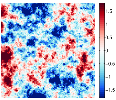
(a) True $\theta=\log(\kappa)$ field.

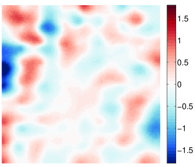
(b) Posterior mean using multiscale approach.

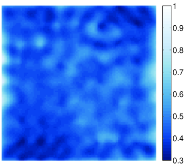
(c) Posterior variance using multiscale approach.

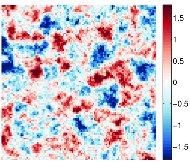
(d) Posterior realization

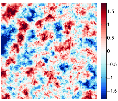
(e) Posterior realization

Fig. 6: Application of the multiscale inference framework to a $10816$-dimensional Bayesian inverse problem.

7 Discussion

We have developed a method for efficiently solving Bayesian inference problems containing multiscale structure, as defined in (2). The method uses transport maps to decouple the original inference problem into a well-conditioned and lower-dimensional coarse-scale sampling problem (sampling $\pi(r_{c}|y)$), followed by direct coarse-to-fine “prolongation” (evaluating $\widetilde{S}_{f}$ with posterior $r_{c}$ samples). By exploiting locality and stationarity, we are able to build these transport maps despite the large dimension of the spatially distributed parameters of interest. Our method accurately approximates the true posterior and can be applied to very large problems that are essentially intractable with other sampling methods. We also stress that our approach is not restricted to subsurface flow applications or elliptic PDE forward models. The construction of transport maps relies entirely on prior samples, and therefore is not problem-specific or tied to specific probability distributions. We should also point out that nothing in our formulation changes when the prior model is hierarchical, e.g., $\pi(\theta|\zeta)$ with some hyperparameters $\zeta$. If the posterior on the hyperparameters is not of particular interest, then marginal samples of $\pi(\theta)=\int\pi(\theta|\zeta)\pi(\zeta)d\zeta$ can directly be generated and our approach used as described. Indeed, exact or approximate satisfaction of the conditional independence assumption (2) is all that is required to apply our framework. Inverse problems with this structure exist in many areas, ranging from tree physiology [24] to materials modeling [45], and numerous other problems with scale separation and/or smoothing forward models.

A typical serial MCMC sampler could take weeks to run on a problem as large as the two-dimensional example from Section 6.2. Decoupling the problem using transport maps allowed us to solve it in only two hours. Part of this improvement lies in the parallelism intrinsic to our approach. All of the prior sampling, much of the optimization used to build the transport maps, and all of the post-MCMC coarse-to-fine map evaluations can be parallelized. This level of parallelism is not available in MCMC samplers, even when multiple chains are run, as MCMC is inherently a serial process. While we used some algorithm-level parallelism (employing MPI for parallel model evaluations and parallel map construction), our approach would lend itself well to more sophisticated distributed-memory or GPU-parallel implementations in the future. Such an implementation could further reduce the run time of our framework.

Of course, allowing our approach to generate approximate posterior samples enables computational savings as well. As demonstrated in Section 5, the accuracy of the posterior approximation can be controlled by the representations of $\widetilde{S}_{c}$ and $\widetilde{S}_{f}$. In Section 6.2, we let $\widetilde{S}_{f}$ be linear in order to mitigate the required computational effort. In applications where more exact posterior sampling is required, however, a higher polynomial degree or alternative functional representation could be employed. Additionally, if problem-specific information is available (such as the locality and stationarity used in Section 5.2.2), it can also be incorporated into the map representation to further increase accuracy and reduce computational expense. This flexibility is important in practice, and should allow our multiscale approach to be applied in diverse areas. Complementing the use of problem-specific information is the development of more advanced map construction techniques, which could adaptively construct and refine maps within a user-specified form, targeting a specified error in (3.3). This is an important area of future research. We emphasize that the fundamental idea underlying our approach—interpreting multiscale structure as conditional independence, and applying it in a Bayesian setting—is independent of the algorithmic specifics of map construction. But advances in the latter will enhance the efficiency and applicability of the inference strategy developed here.

References

- [1] J. E. Aarnes and Y. Efendiev, Mixed multiscale finite element methods for stochastic porous media flows, SIAM Journal on Scientific Computing, 30 (2008), pp. 2319–2339.
- [2] R. Andreani, E. G. Birgin, J. M. Martínez, and M. L. Schuverdt, On Augmented Lagrangian Methods with General Lower-Level Constraints, SIAM Journal on Optimization, 18 (2007), pp. 1286–1309.
- [3] T. Arbogast, Numerical subgrid upscaling of two-phase flow in porous media, Lecture Notes in Phyics, 552 (2000), pp. 35–49.
- [4] R. C. Aster, B. Borchers, and C. H. Thurber, Parameter estimation and inverse problems, Academic Press, 2011.
- [5] J. Bear, Dynamics of Fluids in Porous Media, Dover Publications, 1988.
- [6] L. Biegler, G. Biros, O. Ghattas, M. Heinkenschloss, D. Keyes, B. Mallick, L. Tenorio, B. van Bloemen Waanders, K. Willcox, and Y. Marzouk, Large-scale inverse problems and quantification of uncertainty, vol. 712, John Wiley & Sons, 2011.
- [7] S. Boyd, N. Parikh, E. Chu, B. Peleato, and J. Eckstein, Distributed optimization and statistical learning via the alternating direction method of multipliers, Foundations and Trends in Machine Learning, 3 (2011), pp. 1–122.
- [8] Y. Brenier, Polar factorization and monotone rearrangement of vector-valued functions, Communications on pure and applied mathematics, 44 (1991), pp. 375–417.
- [9] S. Brooks, A. Gelman, G. Jones, and X.-L. Meng, eds., Handbook of Markov Chain Monte Carlo, Chapman and Hall, 2011.
- [10] T. Bui-Thanh and O. Ghattas, Analysis of the Hessian for inverse scattering problems: I. Inverse shape scattering of acoustic waves, Inverse Problems, 28 (2012), p. 055001.
- [11] J. A. Christen and C. Fox, MCMC using an approximation, Journal of Computational and Graphical statistics, 14 (2005), pp. 795–810.
- [12] T. Cui, K. J. Law, and Y. M. Marzouk, Dimension-independent likelihood-informed MCMC, arXiv preprint arXiv:1411.3688, (2014).
- [13] T. Cui, J. Martin, Y. Marzouk, A. Solonen, and A. Spantini, Likelihood-informed dimension reduction for nonlinear inverse problems, Inverse Problems, 30 (2014), p. 114015.
- [14] J. Doherty, L. Brebber, and P. Whyte, PEST: Model-independent parameter estimation, Watermark Computing, Corinda, Australia, 122 (1994).
- [15] P. Dostert, Y. Efendiev, T. Y. Hou, and W. Luo, Coarse-gradient Langevin algorithms for dynamic data integration and uncertainty quantification, Journal of computational physics, 217 (2006), pp. 123–142.
- [16] A. Doucet, N. de Freitas, N. Gordon, and A. Smith, eds., Sequential Monte Carlo in Practice, Springer, 2001.
- [17] W. E, B. Engquist, X. Li, W. Ren, and E. Vanden-Eijnden, Heterogeneous multiscale methods: A review, Communications in Computational Physics, 2 (2007), pp. 367–450.
- [18] Y. Efendiev, T. Hou, and W. Luo, Preconditioning Markov chain Monte Carlo simulations using coarse-scale models, SIAM Journal on Scientific Computing, 28 (2006), pp. 776–803.
- [19] U. EPA, Contaminated Sediment Remediation Guidance for Hazardous Waste Sites, tech. report, United States Environmental Protection Agency, 2005.
- [20] I. Epanomeritakis, V. Akçelik, O. Ghattas, and J. Bielak, A newton-cg method for large-scale three-dimensional elastic full-waveform seismic inversion, Inverse Problems, 24 (2008), p. 034015.
- [21] G. Evensen, Data Assimilation: The Ensemble Kalman Filter, Springer, 2009.
- [22] R. A. Freeze, J. Massmann, L. Smith, T. Sperling, and B. James, Hydrogeological decision analysis: 1. A framework, Groundwater, 28 (1990), pp. 738–766.
- [23] A. Gelman, J. B. Carlin, H. S. Stern, and D. B. Rubin, Bayesian data analysis, vol. 2, Taylor & Francis, 2014.
- [24] I. Graf and J. M. Stockie, Homogenization of the Stefan problem, with application to maple sap exudation, arXiv preprint arXiv:1411.3039, (2014).
- [25] H. Haario, M. Laine, A. Mira, and E. Saksman, DRAM : Efficient adaptive MCMC, Statistics and Computing, 16 (2006), pp. 339–354.
- [26] C. He and L. Durlofsky, Structured flow-based gridding and upscaling for modeling subsurface flow, Advances in Water Resources, (2006), pp. 1876–1892.
- [27] D. Higdon, H. Lee, and Z. Bi, A Bayesian approach to characterizing uncertainty in inverse problems using coarse and fine-scale information, IEEE Transactions on Signal Processing, 50 (2002), pp. 389–399.
- [28] C. H. Holloman, H. K. Lee, and D. M. Higdon, Multiresolution genetic algorithms and Markov chain Monte Carlo, Journal of Computational and Graphical Statistics, 15 (2006).
- [29] T. Hou and Y. Efendiev, Multiscale Finite Element Methods: Theory and Applications, Springer, 2009.
- [30] T. Hughes and G. Sangalli, Variational multiscale analysis: the fine-scale Green s function, projection, optimization, localization, and stabilized methods, SIAM Journal on Numerical Analysis, 45 (2007), p. 539 557.
- [31] T. J. Hughes, G. R. Feijoo, L. Mazzei, and J.-B. Quincy, The variational multiscale method – a paradigm for computational mechanics, Computer Methods in Applied Mechanics and Engineering, 166 (1998), pp. 3–34.
- [32] J. Jagalur Mohan, O. Sahni, A. Doostan, and A. Oberai, Variational multiscale analysis: the fine-scale Green’s function for stochastic partial differential equations, SIAM/ASA Journal on Uncertainty Quantification, 2 (2014), pp. 397–422.
- [33] E. T. Jaynes, Probability Theory: the logic of science., Cambridge University Press, 2003.
- [34] H. Jeffreys, Scientific Inference, Cambridge University Press, 1957.
- [35] P. Jenny, S. Lee, and H. Tchelepi, Multi-scale finite-volume method for elliptic problems in subsurface flow simulation, Journal of Computational Physics, 187 (2003), pp. 47–67.
- [36] , Adaptive fully implicit multi-scale finite-volume method for multi-phase flow and transport in heterogeneous porous media, Journal of Computational Physics, 217 (2006), pp. 627–641.
- [37] R. Juanes and F.-X. Dub, A locally conservative variational multiscale method for the simulation of porous media flow with multiscale source terms., Computational Geosciences, 12 (2008), pp. 273–295.
- [38] J. Kaipio and E. Somersalo, Statistical and Computational Inverse Problems, Springer-Verlag, 2004.
- [39] R. Lewis and V. Torczon, A direct search approach to nonlinear programming problems using an augmented Lagrangian method with explicit treatment of linear constraints, tech. report, College of William & Mary, WM-CS-2010-01, 2010.
- [40] W. Li and O. A. Cirpka, Efficient geostatistical inverse methods for structured and unstructured grids, Water Resources Research, 42 (2006), pp. 1944–7973.
- [41] J. S. Liu, Monte Carlo Strategies in Scientific Computing, Springer, New York, New York, USA, 2004.
- [42] Y. M. Marzouk, T. Moselhy, M. Parno, and A. Spantini, An introduction to sampling via measure transport, in Handbook of Uncertainty Quantification, R. Ghanem, D. Higdon, and H. Owhadi, eds., Springer, 2016.
- [43] Y. M. Marzouk and H. N. Najm, Dimensionality reduction and polynomial chaos acceleration of Bayesian inference in inverse problems, Journal of Computational Physics, 228 (2009), pp. 1862–1902.
- [44] R. McCann, Existence and uniqueness of monotone measure-preserving maps, Duke Mathematical Journal, 80 (1995), pp. 309–323.
- [45] R. E. Miller and E. B. Tadmor, A unified framework and performance benchmark of fourteen multiscale atomistic/continuum coupling methods, Modelling and Simulation in Materials Science and Engineering, 17 (2009), p. 053001.
- [46] J. J. Moré, Generalizations of the trust region problem, Optimization methods and Software, 2 (1993), pp. 189–209.
- [47] T. A. Moselhy and Y. M. Marzouk, Bayesian inference with optimal maps, Journal of Computational Physics, 231 (2012), pp. 7815–7850.
- [48] J. Nolen and G. Papanicolaou, Fine scale uncertainty in parameter estimation for elliptic equations, Inverse Problems, 25 (2009), p. 115021.
- [49] J. Nolen, G. Pavliotis, and A. Stuart, Multiscale modelling and inverse problems, in Numerical Analysis of Multiscale Problems, I. G. Graham, T. Y. Hou, O. Lakkis, and R. Scheichl, eds., Springer Berlin Heidelberg, 2012, pp. 1–34.
- [50] M. Parno, Transport maps for accelerated Bayesian computation, PhD thesis, Massachusetts Institute of Technology, 2014.
- [51] M. Parno, A. Davis, and P. Conrad, MIT Uncertainty Quantification (MUQ) library, 2014. https://bitbucket.org/mituq/muq.
- [52] M. Parno and Y. Marzouk, Transport map accelerated Markov chain Monte Carlo, (2014). arXiv:1412.5492.
- [53] G. Pavliotis and A. Stuart, Multiscale Methods: Averaging and Homogenization, Springer, 2008.
- [54] C. Robert and G. Casella, Monte Carlo Statistical Methods, Springer, New York, New York, USA, 2004.
- [55] G. Roberts and O. Stramer, Langevin diffusions and Metropolis-Hastings algorithms, Methodology and computing in applied probability, (2002), pp. 337–357.
- [56] A. Spantini, A. Solonen, T. Cui, J. Martin, L. Tenorio, and Y. Marzouk, Optimal low-rank approximations of Bayesian linear inverse problems, arXiv preprint arXiv:1407.3463, (2014).
- [57] F. Stavropoulou and J. Muller, A polynomial chaos based Bayesian approach for on-line parameter estimation and control, 2011 IEEE International Symposium on Computer-Aided Control System Design (CACSD), (2011), pp. 1391–1396.
- [58] A. M. Stuart, Inverse problems: A Bayesian perspective, Acta Numerica, 19 (2010), pp. 451–559.
- [59] E. Tabak and C. Turner, A family of nonparametric density estimation algorithms, Communications on Pure and Applied Mathematics, LXVI (2013), p. 145 164.
- [60] E. G. Tabak and E. Vanden-Eijnden, Density estimation by dual ascent of the log-likelihood, Commun. Math. Sci., 8 (2010), pp. 217–233.
- [61] A. Tarantola, Inverse Problem Theory and Methods for Model Parameter Estimation, SIAM, 2005.
- [62] V. V. Vesselinov, D. O. Malley, and D. Katzman, Robust decision analysis for environmental management of groundwater contamination sites, arXiv preprint arXiv:1311.6014, (2013).
- [63] C. Villani, Topics in optimal transportation, American Mathematical Society, 2003.
- [64] , Optimal Transport: Old and New, Springer-Verlag, 2009.
- [65] C. R. Vogel, Computational methods for inverse problems, vol. 23, SIAM, 2002.
- [66] A. Wächter and L. Biegler, On the implementation of an interior-point filter line-search algorithm for large-scale nonlinear programming, Mathematical programming, 106 (2006), pp. 25—-57.
- [67] B. Wagner and S. Gorelick, Reliable aquifer remediation in the presence of spatially variable hydraulic conductivity: From data to design, Water Resources Research, 25 (1989), pp. 2211–2225.
- [68] J. Wan and N. Zabaras, A Bayesian approach to multiscale inverse problems using the sequential Monte Carlo method, Inverse Problems, 27 (2011), p. 105004.
- [69] U. Wolff, Monte carlo errors with less errors, Computer Physics Communications, 156 (2004), pp. 143–153.