monthyeardate[],

The JETSPIN User Manual

M. Lauricella^∗, G. Pontrelli^∗, I. Coluzza^#, D. Pisignano${}^{\text{\textdegree}}$, S. Succi^∗

^∗Istituto per le Applicazioni del Calcolo CNR,

^#Faculty of Physics, University of Vienna,

Boltzmanngasse 5, 1090 Vienna, Austria

${}^{\text{\textdegree}}$Dipartimento di Matematica e Fisica “Ennio De Giorgi”, University of Salento,

version 1.20 - March 3, 2024

Disclaimer

None of the authors, nor any contributor to the JETSPIN code or its derivatives guarantee that the software and associated documentation is free from error. Neither do they accept responsibility for any loss or damage that results from its use. The responsibility for ensuring that the software is fit for purpose lies entirely with the user.

JETSPIN Acknowledgements

The software development process has received funding from the European Research Council under the European Union’s Seventh Framework Programme (FP/2007-2013)/ERC Grant Agreement n. 306357 “NANO-JETS”.

About JETSPIN

The code is licensed under Open Software License v. 3.0 (OSL-3.0). The full text of the licence can be found on the website: http://opensource.org/licenses/OSL-3.0

If results obtained with this code are published, an appropriate citation would be:

Marco Lauricella, Giuseppe Pontrelli, Ivan Coluzza, Dario Pisignano, Sauro Succi, JETSPIN: A specific-purpose open-source software for electrospinning simulations of nanofibers, Submitted to Computer Physics Communications, 2015.

Chapter 1 Introduction

Scope of Chapter

This chapter describes the design and directory structure of JETSPIN.

1.1 The JETSPIN Package

In the recent years, electrospun nanofibers have gained a considerable industrial interest due to many possible applications, such as tissue engineering, air and water filtration, drug delivery and regenerative medicine. In particular, the high surface-area ratio of the fibers offers an intriguing prospect for technological applications. As consequence, several studies were focused on the characterization and production of uni-dimensionally elongated nanostructures. A number of reviews [1, 2, 3, 4, 5] and books [6, 7, 8] concerning electrospinning have been published in the last decade.

Typically, electrospun nanofibers are produced at laboratory scale by the uniaxial stretching of a jet, which is ejected at the nozzle from a charged polymer solution. The initial elongation of a jet can be produced by applying an externally electrostatic field between the spinneret and a conductive collector. Electrospinning involves mainly two sequential stages in the uniaxial elongation of the extruded polymer jet: an initial quasi steady stage, in which the electric field stretches the jet in a straight path away from the nozzle of the ejecting apparatus, and a second stage characterized by a bending instability induced from small perturbations, which misalign the jet from its axis of elongation [9]. These small disturbances may originate from mechanical vibrations at the nozzle or from hydrodynamic-aerodynamic perturbations within the experimental apparatus. Such a misalignment provides an electrostatic-driven bending instability before the jet reaches the conductive collector, where the fibers are finally deposited. As a consequence, the jet path length between the nozzle and the collector increases, and the stream cross-section undergoes a further decrease. The ultimate goal of electrospinning process is to minimize the radius of the collected fibers. By a simple argument of mass conservation, this is tantamount to maximizing the jet length by the time it reaches the collecting plane. By the same argument, it is therefore of interest to minimize the length of the initial stable jet region. Consequently, the bending instability is a desirable effect, as it produces a higher surface-area-to-volume ratio of the jet, which is transferred to the resulting nanofibers [10].

Computational models provide a useful tool to elucidate the physical phenomenon and provide information which might be used for the design of electrospinning experiments. Numerical simulations can be used to improve the capability of predicting the key processing parameters and exert a better control on the resulting nanofiber structure. In recent years, with a renewed interest in nanotechnology, electrospinning studies attracted the attention of many resarchers both from modeling, computational and experimental point of view [11, 12, 13, 14, 15, 9]. Although some author uses dissipative particle dynamics (DPD) mesoscale simulation method into electrospinning study [16], most models usually treat the jet filament as a series of discrete elements (beads) obeying the equations of continuum mechanics [11, 12]. Each bead is subject to different types of interactions, such as long-range Coulomb repulsion, viscoelastic drag, the external electric field. The main aim of such models is to explain the complexity of the resulting dynamics and provide the set of parameters driving the optimal process. The effect of fast-oscillating loads on the bending instability have been explored in an extensive modeling and computational study [17].

JETSPIN delivers a FORTRAN code especially designed to simulate the electrospinning process in a variety of different conditions and experimental settings. This comprehensive platform is devised such that different cases and input variables can be described and simulated. The framework is developed to exploit several computational architectures, both serial and parallel.

JETSPIN, as open-source software, can be used to carry out a systematic sensitivity analysis over a broad range of parameter values. The results of simulations provide valuable insight on the physics of the process and can be used to assess experimental procedures for an optimal design of the equipment and to control processing strategies of technological advanced nanofibers.

1.2 Structure

JETSPIN is written in free format FORTRAN90, and it consists of approximately 160 subroutines. The source exploits the modular approach provided by the programming language. All the variables having in common description of certain features or method are grouped in modules. The convention of explicit type declaration is adopted, and all the arguments passed in calling sequences of functions or subroutines have defined intent. We use the PRIVATE and PUBLIC accessibility attributes in order to decrease error-proneness in programming.

The main routines have been gathered in the main.f90 file, which drives all the CPU-intensive computations needed for the capabilities mentioned below. The variables describing the main features of nanofibers (position, velocity, etc.) are declared in the nanojet_mod.f90 file, which also contains the main subroutines for the memory management of the fundamental data of the simulated system. Since the size system is strictly time-dependent, JETSPIN exploits the dynamic array allocation features of FORTRAN90 to assign the necessary array dimensions. In particular, the size system is modified by the routines add_jetbead and erase_jetbead, while the decision of the main array size, declared as mxnpjet, is handled by the routine reallocate_jet. The sizes of various service bookkeeping arrays are handled within a parallel implementation strategy, witch exploits few dedicated subroutines (see Sec 1.3). All the implemented time integrators are written in the integrator_mod.f90 file, which contains the routine driver_integrator to select the proper integrator, as indicated in the input file. All the terms of equations of motion for the implemented model (see Sec 2.1) are computed by routines located in the eom_mod.f90 file, which call other subroutines in the files coulomb_force_mod.f90, viscoelastic_force_mod.f90 and support_functions_mod.f90. A summarizing scheme of the main JETSPIN program in the main.f90 file has been sketched in Fig 1.1.

The user can carry out simulations of nanofibers without a detailed understanding of the structure of JETSPIN code. All the parameters governing the system can be defined in the input file (see Sec 3.1), which is read by routines located in the io_mod.f90 and parse_mod.f90 files. Instead, the user should be acquainted with the model described in Cap 2. The content of the output file is completely customizable by the input file as described in Sec 3.1, and it can report different time-averaged observables computed by routines of the module statistic_mod (see Sec 3.2). The routines in the error_mod.f90 file can display various warning or error banners on computer terminal, so that the user can easily correct the most common mistakes in the input file.

JETSPIN is supplied as a single UNIX compressed (tarred and gzipped) directory with four sub-directories. All the source code files are contained in the source sub-directory. The examples sub-directory contains different test cases that can help the user to edit new input files. The build sub-directory stores a UNIX makefile that assembles the executable versions of the code both in serial and parallel version with different compilers. Note that JETSPIN may be compiled on any UNIX platform. The makefile should be copied (and eventually modified) into the source sub-directory, where the code is compiled and linked. A list of targets for several common workstations and parallel computers can be used by the command "make target ", where target is one of the options reported in Tab 1.1. On Windows system we advice the user to compile JETSPIN under the command-line interface Cygwin [18]. Finally, the binary executable file can be run in the execute sub-directory.

target:	meaning:
gfortran	compile in serial mode using the GFortran compiler.
gfortran-mpi	compile in parallel mode using the GFortran compiler and the Open Mpi library.
cygwin	compile in serial mode using the GFortran compiler under the command-line
	interface Cygwin for Windows.
cygwin-mpi	compile in parallel mode using the GFortran compiler and the Open Mpi library
	under the command-line interface Cygwin for Windows (note a precompiled
	package of the Open Mpi library is already available on Cygwin).
intel	compile in serial mode using the Intel compiler.
intel-mpi	compile in parallel mode using the Intel compiler and the Intel Mpi library.
intel-openmpi	compile in parallel mode using the Intel compiler and the Open Mpi library.
help	return the list of possible target choices

Table 1.1: List of targets for several common workstations and parallel computers, which can be used by the command "make target".

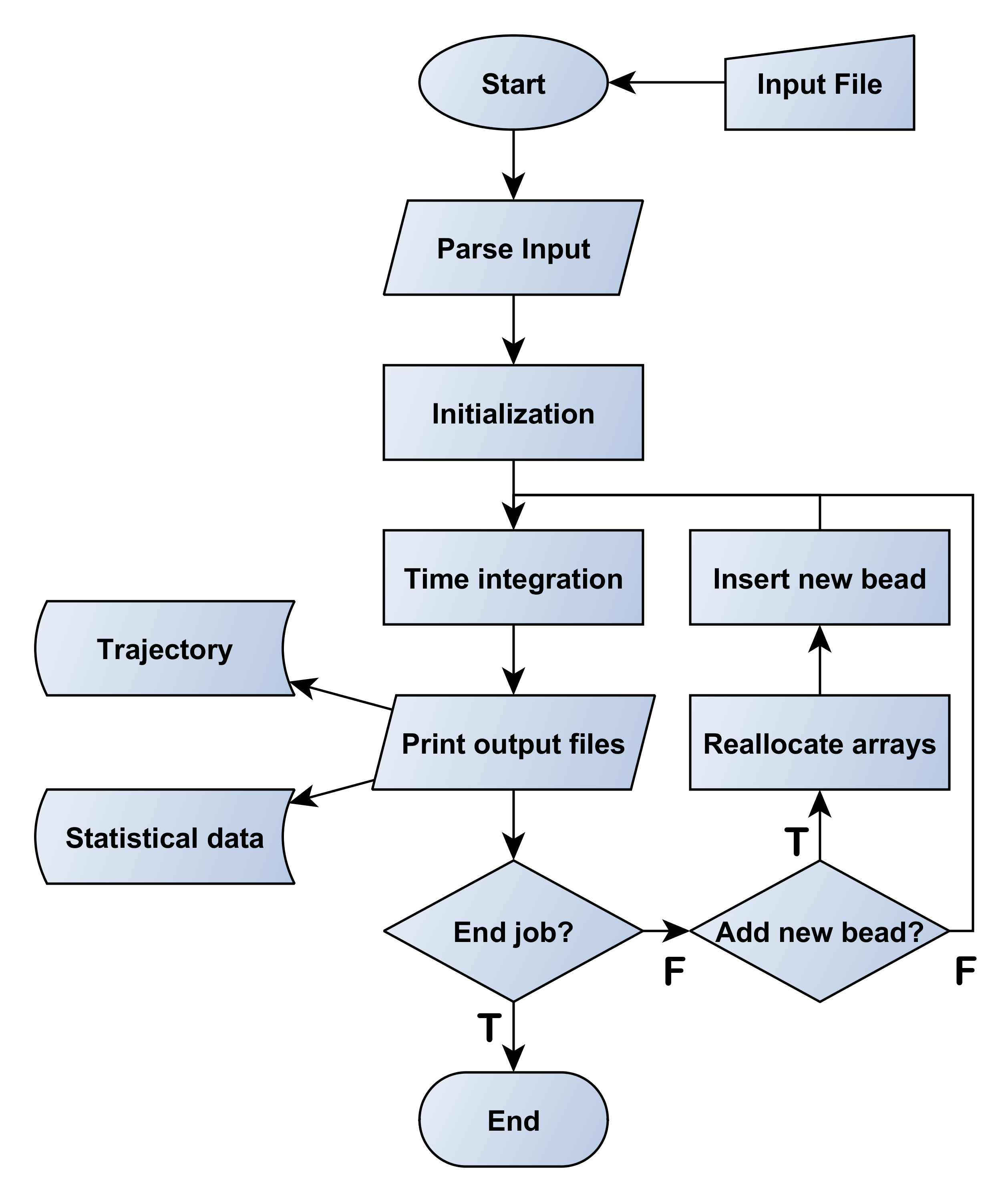
Figure 1.1: Structure of the main JETSPIN program.

1.3 Parallelization

The parallel infrastructure of JETSPIN incorporates the necessary data distribution and communication structures. The parallel strategy underlying JETSPIN is the Replicated Data (RD) scheme[19], where fundamental data of the simulated system are reproduced on all processing nodes. In simulations of nanofibers, the fundamental data consist of position, velocity, and viscoelastic stress arrays of each bead in which the nanojet is discretised (see below Cap 2). Further data defining mass and charge of each bead are also replicated. However, all auxiliary data are distributed in equal portion of data (as much as possible) for each processor. Despite being available other parallel strategies such as the Domain Decomposition[20], our experience has shown that such volume of data is by no means prohibitive on current parallel computers.

By the RD scheme, we adopt in JETSPIN a simple communication strategy of the communication between nodes, which is handled by global summation routines. The module version_mod located in the parallel_version_mod.f90 file contains all the global communication routines which exploit the MPI (Message Passing Interface) library. Note that a FORTRAN90 compiler and an MPI implementation for the specific machine architecture are required in order to compile JETSPIN in parallel mode. An alternative version of the module version_mod is located in the serial_version_mod.f90 file, and it can be easily selected by appropriate flags in the makefile at compile time. By selecting this version, JETSPIN can also be run on serial computers without modification, even though the code has been designed to run on parallel computers.

The size system is strictly time-dependent as mentioned in Sec 1.2 and, therefore, the memory of various service bookkeeping arrays is dynamically distributed over all the processing nodes. In particular, the bookkeeping array size, declared as mxchunk, is managed by the routine set_mxchunk. All the beads of the discretised nanofiber are assigned at every time step to a specific node by the routine set_chunk, and their temporary data are stored in bookkeeping arrays belonging to the assigned node. It is worth stressing that the communication latency makes the parallelization efficiency strictly dependent on the system size. Therefore, we only advice the use of JETSPIN in parallel mode whenever the user expects a system size with at least 50 beads for each node (further details in Ref [21]).

Chapter 2 JETSPIN Model and Algorithms

Scope of Chapter

This chapter describes the model and simulation algorithms incorporated into JETSPIN.

2.1 Equations of Motion

The model implemented in JETSPIN is an extension of the Lagrangian discrete model introduced by Reneker et al. [11] (in the following text referred as Ren model). The model provides a compromise of efficiency and accuracy by representing the filament as a series of $n$ beads (jet beads) at mutual distance $l$ connected by viscoelastic elements. The length $l$ is typically larger than the cross-sectional radius of the filament, but smaller than the characteristic lengths of other observables of interest (e.g. curvature radius). Each $i-th$ bead has mass $m_{i}$ and charge $q_{i}$ (not necessarily equal for all the beads). The nanofiber is modelled as a viscoelastic Maxwell fluid, so that the stress $\sigma_{i}$ for the element connecting bead $i$ with bead $i+1$ is given by the viscoelastic constitutive equation:

$$\frac{d\sigma_{i}}{dt}=\frac{G}{l_{i}}\frac{dl_{i}}{dt}-\frac{G}{\mu}\sigma_{i},$$ (2.1)

where $l_{i}$ is the length of the element connecting bead $i$ with bead $i+1$, $G$ is the elastic modulus, $\mu$ the viscosity of the fluid jet, and $t$ the time. Given $a_{i}$ the cross-sectional radius of the filament at the bead $i$, the viscoleastic force $\vec{\textbf{f}}_{\upsilon e}$ pulling bead $i$ back to $i-1$ and towards $i+1$ is

$$\vec{\textbf{f}}_{\upsilon e,i}=-\pi a_{i}^{2}\sigma_{i}\cdot\vec{\textbf{t}}_{i}+\pi a_{i+1}^{2}\sigma_{i+1}\cdot\vec{\textbf{t}}_{i+1}\text{,}$$ (2.2)

where $\vec{\textbf{t}}_{i}$ is the unit vector pointing bead $i$ from bead $i-1$. The surface tension force $\vec{\textbf{f}}_{st}$ for the $i-th$ bead is given by

$$\vec{\textbf{f}}_{st,i}=k_{i}\cdot\pi\left(\frac{a_{i}+a_{i-1}}{2}\right)^{2}\alpha\cdot\vec{\textbf{c}}_{i}\text{,}$$ (2.3)

where $\alpha$ is the surface tension coefficient, $k_{i}$ is the local curvature, and $\vec{\textbf{c}}_{i}$ is the unit vector pointing the center of the local curvature from bead $i$. Note the force $\vec{\textbf{f}}_{st}$ is acting to restore the rectilinear shape of the bending part of the jet.

In the electrospinning experimental configuration an intense external electric potential $\Phi_{0}$ is applied between the spinneret and a conducting collector located at distance $h$ from the injection point. As consequence, each $i-th$ bead endures the electric force

$$\vec{\textbf{f}}_{el,i}=e_{i}\frac{\Phi_{0}}{h}\cdot\vec{\textbf{x}}\text{,}$$ (2.4)

where $\vec{\textbf{x}}$ is the unit vector pointing the collector from the spinneret and assumed along the $x$ axis. Note that in Ren model the electric field $\Phi$ is assumed to be static in order to avoid the computationally expensive integration of Poisson equation, whereas in reality $\Phi$ is depending on the net charge of the nanofiber so as to maintain constant the potential at the electrodes. The latter issue was elegantly addressed by Kowalewski et al. [22], and its implementation in JETSPIN will be planned.

The net Coulomb force $\vec{\textbf{f}}_{c}$ acting on the $i-th$ bead from all the other beads is given by

$$\vec{\textbf{f}}_{c,i}=\sum_{\begin{subarray}{c}j=1\\ j\neq i\end{subarray}}^{n}\frac{q_{i}q_{j}}{R_{ij}^{2}}\cdot\vec{\textbf{u}}_{ij}\text{,}$$ (2.5)

where $R_{ij}=\left[\left(x_{i}-x_{j}\right)^{2}+\left(y_{i}-y_{j}\right)^{2}+\left(z_{i}-z_{j}\right)^{2}\right]^{1/2}$, and $\vec{\textbf{u}}_{ij}$ is the unit vector pointing the $i-th$ bead from $j-th$ bead.. Although the Ren model provides a reasonable description for the spiral motion of the jet, the last term $\vec{\textbf{f}}_{c}$ introduces mathematical inconsistencies due to the discretization of the fiber into point-charges. Indeed, the charge induces a field on the outer shell of the fiber and not on the center line (as in the implemented model). Different approaches were developed to overcome this issue which usually imply strong approximations[23, 10, 24]. Other strategies use a less crude approximation by accounting for the actual electrostatic form factors between two interacting sections of a charged fiber[25] or involving more sophisticated methods which exploit the tree-code hierarchical force calculation algorithm[22]. The implementation in JETSPIN of methods based on tree-code hierarchical force calculation algorithm will be considered in future.

Although usually much smaller than the other driving forces, the body force due to the gravity is computed in the model by the usual expression

$$\vec{\textbf{f}}_{g,i}=m_{i}g\cdot\vec{\textbf{x}},$$ (2.6)

where $g$ is the gravitational acceleration.

As shown in experimental evidences [26], the air drag force affects the dynamics of the nanofiber. The extended stochastic model developed in Refs [27, 28] was included in JETSPIN to reproduce the aerodynamic effects. In particular, the air drag is modelled by adding two force terms: a random term and a dissipative term. The dissipative air drag term is usually dependent on the geometry of the jet, which changes in time, and it combines longitudinal and lateral components. Based on experimental results[26], the longitudinal component of the air drag dissipative force term acting on bead $i$ is

$$\vec{\textbf{f}}_{air,i}=-0.65\pi a_{i}l_{i}\rho_{a}\left(2a_{i}/\nu_{a}\right)^{-0.81}\upsilon_{tan,i}^{1+0.19}\cdot\vec{\textbf{t}}_{i-1}$$ (2.7)

where $\rho_{a}$ and $\nu_{a}$ are the air density and kinematic viscosity, respectively, $\vec{\textbf{t}}_{i-1}$ is the unit vector pointing bead $i$ from bead $i-1$, and $\upsilon_{tan,i}=\vec{\boldsymbol{\upsilon}_{i}}\cdot\vec{\textbf{t}}_{i-1}$ is the projection of the vector velocity of bead $i$ along the unit vector $\vec{\textbf{t}}_{i-1}$. Further, it is possible to write $\vec{\textbf{f}}_{air,i}$ as

$$\vec{\textbf{f}}_{air,i}=-m_{i}\gamma_{i}\,l_{i}^{0.905}\upsilon_{t,i}^{1+0.19}\cdot\vec{\textbf{t}}_{i-1}$$ (2.8)

if we introduced the dissipative coefficient $\gamma_{i}$ equal to

$$\gamma_{i}=0.65\pi^{0.905}\frac{\rho_{a}}{m_{i}}\left(\frac{2}{\nu_{air}}\right)^{-0.81}V_{i}^{0.095},$$ (2.9)

where $V_{i}=\pi a_{i}^{2}\,l_{i}$ is the jet volume represented by the $i-th$ bead.

Following the expression introduced by A. Yarin[29, 6], under a high-speed air drag the lateral component $\vec{\textbf{f}}_{lift,i}$ of the aerodynamic dissipative force related to the flow speed is given in the linear approximation (for small bending perturbations) by

$$\vec{\textbf{f}}_{lift,i}=-k_{i}\cdot\rho_{a}\upsilon_{i}^{2}\pi\left(\frac{a_{i}+a_{i-1}}{2}\right)^{2}\cdot\vec{\textbf{c}}_{i},$$ (2.10)

where $k_{i}$ is still the local curvature, and $\vec{\textbf{c}}_{i}$ is the unit vector pointing the center of the local curvature from bead $i$. The combined action of such longitudinal and lateral components provide the dissipative force term acting on the $i-th$ bead

$$\vec{\textbf{f}}_{diss,i}=\vec{\textbf{f}}_{air,i}+\vec{\textbf{f}}_{lift,i}\>.$$ (2.11)

Instead, the random force term for the $i-th$ bead has the form

$$\vec{\textbf{f}}_{rand,i}=\sqrt{2m_{i}^{2}D_{\upsilon}}\cdot\vec{\boldsymbol{\eta}_{i}}(t),$$ (2.12)

where $D_{\upsilon}$ denotes a generic diffusion coefficient in velocity space (which is assumed constant and equal for all the beads), and $\vec{\boldsymbol{\eta}_{i}}$ is a three-dimensional vector, whereof each component $\eta$ is an independent stochastic process that is nowhere differentiable with $<\eta\left(t_{1}\right)\eta\left(t_{2}\right)>=\delta\left(\left|t_{2}-t_{1}\right|\right)$, and $<\eta\left(t\right)>=0$. Note that for the sake of simplicity we assume $\eta=d\omega(t)/dt$, where $\omega(t)$ is a Wiener process.

The combined action of these forces governs the elongation of the jet according to the Newton’s equation providing a non-linear Langevin-like stochastic differential equation:

$$m_{i}\frac{d\vec{\boldsymbol{\upsilon}}_{i}}{dt}=\vec{\textbf{f}}_{el,i}+\vec{\textbf{f}}_{c,i}+\vec{\textbf{f}}_{\upsilon e,i}+\vec{\textbf{f}}_{st,i}+\vec{\textbf{f}}_{g,i}+\vec{\textbf{f}}_{diss,i}+\vec{\textbf{f}}_{rand}\>\text{,}$$ (2.13)

where $\vec{\boldsymbol{\upsilon}}_{i}$ is the velocity of the $i-th$ bead. The velocity $\vec{\boldsymbol{\upsilon}}_{i}$ satisfies the kinematic relation:

$$\frac{d\vec{\textbf{r}}_{i}}{dt}=\vec{\boldsymbol{\upsilon}}_{i}$$ (2.14)

where $\vec{\textbf{r}}_{i}$ is the position vector of the $i-th$ bead, $\vec{\textbf{r}}_{i}=x_{i}\vec{\textbf{x}}+y_{i}\vec{\textbf{y}}+z_{i}\vec{\textbf{z}}$. The three Eqs 2.1, 2.13 and 2.14 form the set of equations of motion (EOM) governing the time evolution of system. It is worth stressing that Eq 2.13 recovers a deterministic EOM by imposing $\rho_{a}=0$ and $D_{\upsilon}=0$.

2.2 Perturbations at the nozzle

The spinneret nozzle is represented by a single mass-less point of charge $\bar{q}$ fixed at $x=0$ (nozzle bead). Its charge $\bar{q}$ is assumed equal to the mean charge value of the jet beads. Such charged point can be also interpreted as a small portion of jet which is fixed to the nozzle. In JETSPIN it is possible to add small perturbations to the $y_{n}$ and $z_{n}$ coordinates of the nozzle bead in order to model fast mechanical oscillations of the spinneret[17]. Given the initial position of the nozzle

$$y_{n}=A\cdot\cos\left(\varphi\right)$$ (2.15a)

$$z_{n}=A\cdot\sin\left(\varphi\right),$$ (2.15b)

the equations of motion for the nozzle bead are

$$\frac{dy_{n}}{dt}=-\omega\cdot z_{n}$$ (2.16a)

$$\frac{dz_{n}}{dt}=\omega\cdot y_{n},$$ (2.16b)

where $A$ denotes the amplitude of the perturbation, while $\omega$ and $\varphi$ are its frequency and initial phase, respectively.

2.3 Jet insertion

The jet insertion at the nozzle is modelled as follows. For the sake of simplicity, let us consider a simulation which starts with only two bodies: a single mass-less point fixed at $x=0$ representing the spinneret nozzle, and a bead modelling an initial jet segment of mass $m_{i}$ and charge $e_{i}$ located at distance $l_{step}$ from the nozzle along the $x$ axis. Here, $l_{step}$ denotes the length step used to discretise the jet in a sequence of beads. The starting jet bead is assumed to have a cross-sectional radius $a_{0}$, defined as the radius of the filament at the nozzle before the stretching process. Applying the condition that the volume of the jet is conserved, the relation $\pi a_{i}^{2}\,l_{i}=\pi a_{0}^{2}l_{step}$ is valid for any $i-th$ bead. Furthermore, the starting jet bead has an initial velocity $\upsilon_{s}$ along the $x$ axis equal to the bulk fluid velocity in the syringe needle. Once this traveling jet bead is a distance of $2\cdot l_{step}$ away from the nozzle, a new jet bead (third body) is placed at distance $l_{step}$ from the nozzle along the straight line joining the two previous bodies. Let us now label $i-1$ the farthest bead from the nozzle, and $i$ the last inserted bead. The $i-th$ bead is inserted with the initial velocity $\upsilon_{i}=\upsilon_{s}+\upsilon_{d}$, where $\upsilon_{d}$ denotes the dragging velocity computed as

$$\upsilon_{d}=\frac{\upsilon_{i-i}-\upsilon_{s}}{2}.$$ (2.17)

Here, the dragging velocity should be interpreted as an extra term which accounts for the drag effect of the electrospun jet on the last inserted segment. Note that the actual dragging velocity definition was chosen in order to not alter the strain velocity term $\left(1/l_{i-1}\right)\cdot\left(dl_{i-1}/dt\right)$ of Eq 2.1 before and after the bead insertion.

2.4 Dynamic refinement

In the original Ren model, each bead represent a constant quantity $V_{c}$ of jet volume, so that the relationship $\pi a_{i}^{2}\,l_{i}=\pi a_{0}^{2}l_{step}=V_{c}$ is valid for any $i-th$ bead. Despite such relationship can be sometimes a useful advantage (as example, see Sec 2.5), the radius reduction $a_{i}$ of the electrospun nanofiber provides a significant increase of the discretization length $l_{i}$ value along the jet path (also greater than two order of magnitude). As consequence, it was observed in literature [22] that the jet discretization close the collector becomes rather coarse to model efficiently the nanofiber. To get around this problem a dynamic refinement can be used in JETSPIN in order to maintain the the length of the elements $l_{i}$ below a prescribed characteristic length max $l_{max}$. Whenever a bead length $l_{i}$ is larger than $l_{max}$, the nanofiber is refined by discretizing uniformly the jet at the length step $l_{step}$ value given in input file. The discretization is performed by Akima spline interpolations [30, 31] of the main quantities describing the jet beads (positions, fiber radius, stress, velocities). In order to perform the interpolation we proceed as follows: First of all, we introduce the variable $\lambda\in[0,1]$ to parametrize the jet path, where $\lambda=0$ identifies the nozzle, and $\lambda=1$ the jet at the collector. For each bead we compute its respective $\lambda_{i}$ value by using the formula

$$\lambda_{i}=\frac{1}{l_{path}}\sum_{k=1}^{i}l_{k}$$ (2.18)

where $l_{path}=\sum_{k=1}^{N_{beads}}l_{k}$ is the jet path length from the nozzle to the collector, and $i=1$ and $i=N_{beads}$ denote the jet bead at the nozzle and collector, respectively ($i=0$ denotes the nozzle). The set of ${\lambda_{i}}$ values represent the mesh used to build the cubic spline. Given a generic quantity $y$, the data $y_{i}=y\left(\lambda_{i}\right)$ are tabulated and used in order to compute the coefficients of the Akima spline, following the algorithm reported in Ref [31]. Then, we enforce a uniform parametrization of the nanofiber by imposing all the lengths of the elements equal to $l_{step}$. The new mesh ${\lambda_{i}^{*}}$ is defined as

$$\lambda_{0}^{*}=0\;\lambda_{i}^{*}=\frac{i}{N_{beads}^{*}},\;i=1,2,\ldots,N_{beads}^{*}\text{.}$$ (2.19)

where $N_{beads}^{*}=l_{path}/l_{step}$ represents the number of jet beads in the new representation. Finally, the new values $y\left(\lambda_{i}^{*}\right)$ are computed for any $i-th$ bead by the spline interpolation. The procedure is repeated for positions, fiber radius, stress and velocities of the jet beads in order to provide the respective quantities in the new mesh ${\lambda_{i}^{*}}$. It is worth to sressing that the volume $V_{i}=\pi a_{i}^{2}\,l_{i}$ represented by each bead is not anymore constant, and, consequently, $\pi a_{i}^{2}\,l_{i}\neq\pi a_{0}^{2}l_{step}$. In the following text we will refer to this emended version of the Ren model as DyRen model.

2.5 Dimensionless quantities

In JETSPIN all the variables are automatically rescaled and stored in dimensionless units. In order to adopt a dimensionless form of the equations of motion, we use the dimensionless scaling procdure proposed by Reneker et al.[11]. We define a characteristic length

$$L_{0}=\sqrt{\frac{\bar{q}^{2}}{\pi a_{0}^{2}G}}=l_{step}\sqrt{\frac{\pi a_{0}^{2}\rho_{V}^{2}}{G}},$$ (2.20)

where we write the charge $q$ as $\pi a_{0}^{2}l_{step}\rho_{V}$, denoting $\rho_{V}$ the electric volume charge density of the filament. Further, we divide the time $t$ and the stress $\sigma$ by their respective characteristic scales reported in Tab2.1. Applying the condition that the volume of the jet is conserved $\pi a_{i}^{2}\,l_{i}=V_{i}$ for any $i-th$ bead, we rewrite the EOM as:

$$\frac{d\vec{\bar{\textbf{r}}}_{i}}{d\bar{t}}=\vec{\boldsymbol{\bar{\upsilon}}}_{\,i}$$ (2.21a)

$$\frac{d\bar{\sigma}_{i}}{d\bar{t}}=\frac{1}{\bar{l}_{i}}\frac{d\bar{l}_{i}}{d\bar{t}}-\bar{\sigma}_{i}$$ (2.21b)

$$\frac{d\vec{\boldsymbol{\bar{\upsilon}}}_{\,i}}{d\bar{t}}= \Phi\cdot\vec{\textbf{x}}+\sum_{\begin{subarray}{c}j=1\\ j\neq i\end{subarray}}^{n}\frac{Q_{ij}}{\bar{R}_{ij}^{2}}\cdot\vec{\textbf{u}}_{ij}-F_{ve,i}\bar{V}_{i}\frac{\bar{\sigma}_{i}}{\bar{l}_{i}}\cdot\vec{\textbf{t}}_{i}+F_{ve,i+1}\bar{V}_{i+1}\frac{\bar{\sigma}_{i+1}}{\bar{l}_{i+1}}\cdot\vec{\textbf{t}}_{i+1}$$ (2.21c)

$$+A_{i}\frac{\bar{k_{i}}}{4}\left(\frac{\sqrt{\bar{V}_{i}}}{\sqrt{\bar{l}_{i}}}+\frac{\sqrt{\bar{V}_{i-1}}}{\sqrt{\bar{l}_{i-1}}}\right)^{2}\cdot\vec{\textbf{c}}_{i}+F_{g}\cdot\vec{\textbf{x}}-\Gamma_{i}\,\bar{l}_{i}^{0.905}\bar{\upsilon}_{tan,i}^{1+0.19}\cdot\vec{\textbf{t}}_{i-1}-$$

$$-\Lambda_{i}\frac{\bar{k_{i}}\bar{\upsilon}_{tan,i}^{2}}{4}\left(\frac{\sqrt{\bar{V}_{i}}}{\sqrt{\bar{l}_{i}}}+\frac{\sqrt{\bar{V}_{i-1}}}{\sqrt{\bar{l}_{i-1}}}\right)^{2}\cdot\vec{\textbf{c}}_{i}+\sqrt{2\Theta_{\upsilon}}\cdot\vec{\boldsymbol{\eta}_{i}}(\bar{t})$$

where we used the dimensionless derived variables and groups defined in Tab2.1. It is worth stressing that the viscoelastic and surface tension force terms are slightly different from the dimensionless form provided by Reneker et al. [11], since we are considering the DyRen model presented in Sec 2.4. In particular, we do not use the relation $\pi a_{i}^{2}\,l_{i}=\pi a_{0}^{2}l_{step}$ since it is valid only for the Ren model (see discussion in Sec 2.4).

Finally, the dimensionless EOM of the nozzle are given as

$$\frac{d\bar{y}_{i}}{d\bar{t}}=-K_{s}\cdot\bar{z}_{i}$$ (2.22a)

$$\frac{d\bar{z}_{i}}{d\bar{t}}=K_{s}\cdot\bar{y}_{i}\>,$$ (2.22b)

with the dimensionless parameter $K_{s}$ defined in Tab2.1.

Characteristic Scales
$L_{0}=l_{step}\sqrt{\frac{\pi a_{0}^{2}\rho_{V}^{2}}{G}}$	$t_{0}=\frac{\mu}{G}$
$\sigma_{0}=G$
Dimensionless Quantities
$\bar{l}_{i}={\displaystyle\frac{l_{i}}{L_{0}}}$	$\bar{R}_{ij}={\displaystyle\frac{R_{ij}}{L_{0}}}$
$\bar{\sigma}_{i}={\displaystyle\frac{\sigma_{i}}{\sigma_{0}}}$	$\bar{\upsilon}_{i}=\upsilon_{i}{\displaystyle\frac{t_{0}}{L_{0}}}$
$\bar{k_{i}}=k_{i}L_{0}$	$\bar{\upsilon}_{tan,i}=\upsilon_{tan,i}{\displaystyle\frac{t_{0}}{L_{0}}}$
$\bar{V}_{i}={\displaystyle\frac{V_{i}}{L_{0}^{3}}}$
Dimensionless Groups
$\Phi_{i}={\displaystyle\frac{q_{i}\Phi_{0}\mu^{2}}{m_{i}h\,L_{0}\,G^{2}}}$	$Q_{ij}={\displaystyle\frac{q_{i}q_{j}\mu^{2}}{m_{i}L_{0}^{3}G^{2}}}$
$F_{ve,i}={\displaystyle\frac{L_{0}\mu^{2}}{m_{i}G}}$	$A_{i}={\displaystyle\frac{\alpha\mu^{2}}{m_{i}G^{2}}}$
$F_{g}={\displaystyle\frac{g\mu^{2}}{L_{0}G^{2}}}$	$K_{s}=\omega{\displaystyle\frac{\mu}{G}}$
$H={\displaystyle\frac{h}{L_{0}}}$	$L_{step}={\displaystyle\frac{l_{step}}{L_{0}}}$
$\Gamma_{i}={\displaystyle\gamma_{i}\cdot t_{0}L_{0}^{0.905}\left(\frac{L_{0}}{t_{0}}\right)^{0.19}}$	$\Theta_{\upsilon}=D_{\upsilon}\cdot{\displaystyle\frac{t_{0}^{3}}{L_{0}^{2}}}$
$\Lambda_{i}={\displaystyle\frac{\rho_{a}L_{0}^{2}}{m_{i}}}$

Table 2.1: Definitions of the characteristic scales, dimensionless derived variables, and groups employed in the text.

2.6 Integration schemes

In order to integrate the homogeneous differential equations of motion we discretise time as $t_{i}=t_{0}+i\Delta t$ with $i=1,\ldots,n_{steps}$, where $n_{steps}$ denotes the number of sub-intervals. Note that in JETSPIN the time step $\Delta t$ is automatically rescaled by the quantity $\tau$, in accordance with the mentioned dimensionless scaling convention. Three different integration schemes are available for deterministic simulations: the first-order accurate Euler scheme, the second-order accurate Heun scheme (sometimes called second-order accurate Runge-Kutta), and the fourth-order accurate Runge-Kutta scheme[32]. The user can select a specific scheme by using appropriate keys in the input file, as described in Sec 3.1. For the integration of stochastic simulations the explicit strong order scheme by Platen [33, 34, 35] was implemented, whereof the order of strong convergence was evaluated equal to 1.5. This scheme avoids the use of derivatives by corresponding finite differences in the same way as Runge-Kutta schemes do for ODEs in a deterministic setting, and it is briefly summarized as follows.

Let us consider a Brownian motion vector process $\textbf{X}=\left\{\textbf{X}_{t},t\right\}$ of d-dimensional satisfying the stochastic differential equation

$$\frac{d\textbf{X}}{dt}=\textbf{a}\left(t,X^{1},\ldots,X^{d}\right)+\textbf{b}d\Omega$$ (2.23)

where a and b are vectors of d-dimensional usually called drift and diffusion vector coefficients, and $\Omega\left(t\right)$ denotes a Wiener process. Denoted $Y_{t}^{k}$ the approximation for the k-th component of the vector X at time $t$, the integrator has the following form:

$$Y_{t+\varDelta t}^{k}=Y_{t}^{k}+b^{k}\Delta\Omega+\frac{1}{2\sqrt{\Delta t}}\left[a^{k}\left(\widetilde{\boldsymbol{\Upsilon}}_{+}\right)-a^{k}\left(\widetilde{\boldsymbol{\Upsilon}}_{-}\right)\right]\Delta\varPsi+\frac{1}{4}\left[a^{k}\left(\widetilde{\boldsymbol{\Upsilon}}_{+}\right)+2a^{k}+a^{k}\left(\widetilde{\boldsymbol{\Upsilon}}_{-}\right)\right]\Delta t,$$ (2.24)

with the vector supporting values

$$\widetilde{\boldsymbol{\Upsilon}}_{\pm} =\textbf{Y}_{t}+\textbf{a}\Delta t\pm\textbf{b}\sqrt{\Delta t}$$ (2.25)

$$\widetilde{\boldsymbol{\Phi}}_{\pm} =\widetilde{\boldsymbol{\Upsilon}}_{+}\pm\textbf{b}\left(\widetilde{\boldsymbol{\Upsilon}}_{+}\right)\sqrt{\Delta t}.$$

Here, $\Delta\Omega$ and $\Delta\varPsi$ indicate normally distributed random variables constructed from two independent $N\left(0,1\right)$ standard Gaussian distributed random variables ($U_{1}$, $U_{2}$) by means of the following linear transformation:

$$\Delta\Omega =U_{1}\sqrt{\Delta t}$$ (2.26)

$$\Delta\varPsi =\frac{1}{2}\Delta t^{3/2}\left(U_{1}+\frac{1}{\sqrt{3}}U_{2}\right).$$

Chapter 3 JETSPIN Data Files

Scope of Chapter

This chapter describes all the input and output files of JETSPIN.

3.1 Input file

In order to run JETSPIN simulations an input file has to be prepared, which is a free-format and case-insensitive. The input file has to be named input.dat, and it contains the selection of the model system, integration scheme directives, specification of various parameters for the model, and output directives. The input file does not requires a specific order of key directives, and it is read by the input parsing module. Every line is treated as a command sentence (record). Records beginning with the symbol # (commented) and blank lines are not processed, and may be added to aid readability. Each record is read in words (directives and additional keywords and numbers), which are recognized as such by separation by one or more space characters.

As in the example given in input test, the last record is a finish directive, which marks the end of the input data. Before the finish directive, a wide list of directives may be inserted (see Tab 3.1). The key systype should be used to set the nanofiber model. In JETSPIN two models are available: 1) the one dimensional model similar to the model of Cap 2 but assuming the nanofiber to be straight along the $\vec{\textbf{x}}$ axis, and, therefore, neglecting the surface tension force $\vec{\textbf{f}}_{st}$; 2) the three dimensional model described in Cap 2. Internally these options are handled by the integer variable systype, which assumes the values explained in Tab 3.1. Further details of the 1-D model can be found in Refs [36, 37]. A series of variables are mandatory and have to be defined. For example, timestep, final time, initial length, etc. (see underlined directives in Tab 3.1). A missed definition of any mandatory variable will call an error banner on the terminal. The user can use two possible ways to define the initial geometry of a nanofiber both given the mandatory directive initial length: 1) the discretization step length of nanofiber is specified by the directive resolution, which causes automatically the setting of the jet segments number (the number of segment in which the jet is discretised); 2) the jet segments number is declared by the directive points, while the value of the discretization step length is automatically set by the program (as in Example Test Case 3 in Sec 4.3). The directive cutoff indicates the length of the upper and lower proximal jet sections, which interact via Coulomb force on any bead. It is worth stressing that the length value is set at the nozzle, so that the effective cutoff increases along the simulation as the nanofiber is stretched.

The user should pay special attention in choosing the time integration step given by the directive timestep, whose detailed considerations are provided in Ref [21]. The reader is referred to Tab 3.1 for a complete listing of all directives defining the electrospinning setup parameters. Not all these quantities are mandatory, but the user is informed that whenever a quantity is missed, it is usually assumed equal to zero by default (exceptions are stressed in Tab 3.1). Note all the quantities have to be expressed in centimeter–gram–second unit system (e.g. charge in statcoulomb, electric potential in statvolt, etc.).

directive:	meaning:
airdrag yes	active the inclusion of the airdrag force in the model
	(note that if yes the directive “integrator 4” is mandatory)
airdrag airdensity $f$	mass density of the air surrounding the nanofiber (default: 0)
airdrag airviscosity $f$	kinematic viscosity of the air surrounding the nanofiber (default: 1)
airdrag airvelocity $f$	velocity of the air with respect to the z axis (default: 0)
airdrag amplitude $f$	amplitude of the randomic force rescaled by $\gamma$ (default: 1)
	(note that the dissipation coefficient $\gamma$ is automatically
	computed by JETSPIN using the input data)
collector distance $f$	distance of collector along the x axis from the nozzle
	(note the nozzle is assumed in the origin)
cutoff $f$	length of the proximal jet sections interacting by Coulomb
	force (default: equal to the collector distance)
density mass $f$	mass density of the nanofiber
density charge $f$	electric volume charge density of the nanofiber
dynam refin yes	active the dynamic refinement during the simultion
dynam refin threshold $f$	set the threshold beyond which the refinement is applied
dynam refin every $f$	the refinement is applied every $f$ seconds
dynam refin start $f$	the refinement is applied only if the simulation time is greater
	than or equal to $f$ seconds
elastic modulus $f$	elastic modulus of the nanofiber
external potential $f$	electric potential between the nozzle and collector
final time $f$	set the end time of the simulation
finish	close the input file (last data record)
gravity yes	active the inclusion of the gravity force in the model
initial length $f$	length of the nanofiber at the initial time
integrator $i$	set the integration scheme. The integer can be ’1’ for
	Euler, ’2’ for Heun, ’3’ for Runge-Kutta, and ’4’
	for the Platen scheme (only for airdrag force activated).
inserting yes	inject new beads as explained in Subsec
nozzle cross $f$	cross section radius of the nanofiber at the nozzle
nozzle stress $f$	viscoelastic stress of the nanofiber at the nozzle
nozzle velocity $f$	bulk fluid velocity of the nanofiber at the nozzle
perturb yes	active the periodic perturbation at the nozzle
perturb freq $f$	frequency of the perturbation at the nozzle
perturb ampl $f$	amplitude of the perturbation at the nozzle
points $i$	number of segment in which the jet is discretised
print list $s_{1}\,\ldots$	print on terminal statistical data as indicated by symbolic
	strings (see Tab 3.2 for detailed informations)
print time $f$	print data on terminal and output file every $f$ seconds
print xyz $f$	print the trajectory in XYZ file format in centimeters
	every $f$ seconds
print xyz frame $f$	print the jet geometry in a single XYZ file format in centimeters
	every $f$ seconds (default name of files: frame%06d.xyz)
print xyz maxnum $i$	print the XYZ file format with $i$ beads starting from the
	nearest bead to the collector (default: 100)
print xyz rescale $f$	print the XYZ file format data rescaled by $f$
printstat list $s_{1}\,\ldots$	print on output file statistical data as indicated by symbolic
	strings (see Tab 3.2 for detailed informations)
removing yes	remove beads at collector
resolution $f$	discretization step length of nanofiber
seed $i$	seed control to the internal random number generator
surface tension $f$	surface tension coefficient of the nanofiber
system $i$	set the nanofiber model. The integer can be equal to
	’1’ for select the 1d-model or ’3’ for the 3d-model
timestep $f$	set the time step for the integration scheme
viscosity $f$	viscosity of the nanofiber

Table 3.1: Here, we report the list of directives available in JETSPIN. Note $i$, $f$, and $s$ denote an integer number, a floating point number, and a string, respectively. The underlined directives are mandatory. The default value is zero (exceptions are stressed in parentheses).

3.2 Output files

A series of specific directives causes the writing of output files (see Tab 3.1). In JETSPIN three output files can be written: 1) the file statdat.dat containing time-dependent statistical data of simulated process; 2) the file traj.xyz reporting the nanofiber trajectory in XYZ format file; 3) the files frame%06d.xyz reporting the nanofiber geometries in splitted XYZ format files (a single file for each frame).

Various statistical data can be written on the file statdat.dat , and the user can select them in input using the directive printstat list followed by appropriate symbolic strings, whose the list with corresponding meanings is reported in Tab 3.2. The selected observables will be printed at time interval on the same line following the order specified in input file. In the same way, a list of statistical data can be printed on computer terminal using the directive print list followed by the symbolic strings of Tab 3.2.

The file traj.xyz is written as a continuous series of XYZ format frames taken at time interval, so that can be read by suitable visualization programs (e.g. VMD-Visual Molecular Dynamics [38], UCSF Chimera [39], etc.) to generate animations. The number of elements contained in the file is kept constant equal to the value specified by the directive print xyz maxnum, since few programs (e.g. VMD) do not manage a variable number of elements along the simulations. If the actual number of beads is lower than the given constant maxnum, the extra elements are printed in the origin point.

keys:	meaning:
t	unscaled time
ts	scaled time
x, y, z	unscaled coordinates of the farest bead
xs, ys, zs	scaled coordinates of the farest bead
st	unscaled stress of the farest bead
sts	scaled stress of the farest bead
vx, vy, vz	unscaled velocities of the farest bead
vxs, vys, vzs	scaled velocities of the farest bead
yz	unscaled normal distance from the x axis of the farest bead
yzs	scaled normal distance from the x axis of the farest bead
mass	last inserted mass at the nozzle
q	last inserted charge at the nozzle
cpu	time for every print interval
cpur	remaining time to the end
cpue	elapsed time
n	number of beads used to discretise the jet
f	index of the first bead
l	index of the last bead
curn	current at the nozzle
curc	current at the collector
vn	velocity modulus of jet at the nozzle
vc	velocity modulus of jet at the collector
svc	strain velocity at the collector
mfn	mass flux at the nozzle
mfc	mass flux at the collector
rc	radius of jet at the collector
rrr	radius reduction ratio of jet
lp	length path of jet
rlp	length path of jet divided by the collector distance

Table 3.2: In JETSPIN a series of instantaneous and statistical data are available to be printed by selecting the appropriate key. Here, the list of symbolic string keys is reported with their corresponding meanings. Note by scaled we mean that the observable was rescaled by the characteristic values provided in Tab2.1. The underlined keys correspond to data which are averaged on the time interval given by the directive print time in input file. Note by farest bead we mean the farest bead from the nozzle (with greatest $x$ value). Note all the quantities are expressed in centimeter–gram–second unit system, excepted the dimensionless scaled observables.

Chapter 4 Example Simulations

Scope of Chapter

This chapter describes the standard test cases for JETSPIN, the input and output files for which are in the examples sub-directory.

4.1 Test Case 1: 1-D case

This input file (located in the input-1 sub-directory) provides the dimensionless parameter values $Q=12$, $V=2$ and $F_{ve}=12$, which have been already used as reference case in Refs [11, 36].

4.2 Test Case 2: 1-D case with bead insertion at the nozzle activated

This input file (located in the input-2 sub-directory) provides the dimensionless parameter values $Q=12$, $V=2$ and $F_{ve}=12$, as in the previous test case, but here we have activated the injection of new beads by the directive inserting yes in the input file.

4.3 Test Case 3: Three-D simulations of a process leading to polymer nanofibers

The electrospinning of polyvinylpyrrolidone (PVP) nanofibers is a prototypical process, which has been largely investigated in literature.[6, 8, 5] By the input located in the input-3 sub-directory, we simulate the electrospinning process of PVP solutions. Then, the theoretical results predicted by the models are compared with the aforementioned experimental data. In particular, we reproduce an experiment in which a solution of PVP (molecular weight = 1300 kDa) is prepared by a mixture of ethanol and water (17:3 v:v), at a concentration of about 2.5 wt%. The applied voltage is in a range around 10 kV, and the collector is placed at distance 16 cm from the nozzle, which has radius $250\,$micron (further details are provided in Ref. [40, 21] ). As rheological properties of such system we consider the zero-shear viscosity $\mu_{0}=0.2\,\text{g}/(\text{cm}\cdot\text{s})$ [41, 42], the elastic modulus $G=5\cdot 10^{4}\,\text{g}/(\text{cm}\cdot\text{s}^{2})$ [43], and the surface tension $\alpha=21.1\,\text{g}/\text{s}^{2}$ [41]. We use for the simulation a viscosity value $\mu$ which is two order of magnitude larger than the zero-shear viscosity $\mu_{0}$ reported, since the strong longitudinal flows we are dealing with can lead to an increase of the extensional viscosity from $\mu_{0}$, as already observed in literature.[11, 29] The mass density is equal to $0.84\,\text{g}/\text{cm}^{3}$, while the charge density was estimated by experimental observations of the current measured at the nozzle. For convenience, all the simulation parameters are summarized in Tab4.1.

$\rho$	$\rho_{q}$	$a_{0}$	$\upsilon_{s}$	$\alpha$	$\mu$	$G$	$V_{0}$	$\omega$	$A$
($\text{kg}/\text{m}^{3}$)	($\text{C}/\text{L}$)	(cm)	(cm/s)	(mN/m)	(Pa$\cdot$s)	(Pa)	(kV)	($\text{s}^{-1}$)	(cm)
840	$2.8\cdot 10^{-7}$	$5\cdot 10^{-3}$	0.28	21.1	2.0	50000	9.0	$10^{4}$	$10^{-3}$

Table 4.1: Simulation parameters for the simulation of PVP nanofibers. The headings used are as follows: $\rho$: density, $\rho_{q}$: charge density, $a_{0}$: fiber radius at the nozzle, $\upsilon_{s}$: bulk fluid velocity in the syringe needle, $\alpha$: surface tension, $\mu$: viscosity, $G$ : elastic modulus, $V_{0}$ : applied voltage bias, $\omega$: frequency of perturbation, $A$ : amplitude of perturbation. The bulk fluid velocity $\upsilon_{s}$ was estimated considering that the solution was pumped at constant flow rate of 2 mL/h in a needle of radius $250\,$micron.

References

- [1] D. Li, Y. Wang, Y. Xia, Electrospinning nanofibers as uniaxially aligned arrays and layer-by-layer stacked films, Advanced Materials 16 (4) (2004) 361–366.
- [2] A. Greiner, J. H. Wendorff, Electrospinning: a fascinating method for the preparation of ultrathin fibers, Angewandte Chemie International Edition 46 (30) (2007) 5670–5703.
- [3] C. P. Carroll, E. Zhmayev, V. Kalra, Y. L. Joo, Nanofibers from electrically driven viscoelastic jets: modeling and experiments, Korea-Aust Rheol J 20 (2008) 153–164.
- [4] Z.-M. Huang, Y.-Z. Zhang, M. Kotaki, S. Ramakrishna, A review on polymer nanofibers by electrospinning and their applications in nanocomposites, Composites science and technology 63 (15) (2003) 2223–2253.
- [5] L. Persano, A. Camposeo, C. Tekmen, D. Pisignano, Industrial upscaling of electrospinning and applications of polymer nanofibers: a review, Macromolecular Materials and Engineering 298 (5) (2013) 504–520.
- [6] A. L. Yarin, B. Pourdeyhimi, S. Ramakrishna, Fundamentals and Applications of Micro and Nanofibers, Cambridge University Press, 2014.
- [7] J. H. Wendorff, S. Agarwal, A. Greiner, Electrospinning: materials, processing, and applications, John Wiley & Sons, 2012.
- [8] D. Pisignano, Polymer Nanofibers: Building Blocks for Nanotechnology, Royal Society of Chemistry, 2013.
- [9] Y. Zeng, Y. Wu, Z. Pei, C. Yu, Numerical approach to electrospinning, International Journal of Nonlinear Sciences and Numerical Simulation 7 (4) (2006) 385–388.
- [10] J. Feng, Stretching of a straight electrically charged viscoelastic jet, Journal of Non-Newtonian Fluid Mechanics 116 (1) (2003) 55–70.
- [11] D. H. Reneker, A. L. Yarin, H. Fong, S. Koombhongse, Bending instability of electrically charged liquid jets of polymer solutions in electrospinning, Journal of Applied physics 87 (9) (2000) 4531–4547.
- [12] A. L. Yarin, S. Koombhongse, D. H. Reneker, Taylor cone and jetting from liquid droplets in electrospinning of nanofibers, Journal of Applied Physics 90 (9) (2001) 4836–4846.
- [13] S. V. Fridrikh, H. Y. Jian, M. P. Brenner, G. C. Rutledge, Controlling the fiber diameter during electrospinning, Physical review letters 90 (14) (2003) 144502.
- [14] S. Theron, E. Zussman, A. Yarin, Experimental investigation of the governing parameters in the electrospinning of polymer solutions, Polymer 45 (6) (2004) 2017–2030.
- [15] C. Lu, P. Chen, J. Li, Y. Zhang, Computer simulation of electrospinning. part i. effect of solvent in electrospinning, Polymer 47 (3) (2006) 915–921.
- [16] X. Wang, Y. Liu, C. Zhang, Y. An, X. He, W. Yang, Simulation on electrical field distribution and fiber falls in melt electrospinning, Journal of nanoscience and nanotechnology 13 (7) (2013) 4680–4685.
- [17] I. Coluzza, D. Pisignano, D. Gentili, G. Pontrelli, S. Succi, Ultrathin fibers from electrospinning experiments under driven fast-oscillating perturbations, Physical Review Applied 2 (5) (2014) 054011.
- [18] J. Racine, The cygwin tools: a gnu toolkit for windows, Journal of Applied Econometrics 15 (3) (2000) 331–341.
- [19] W. Smith, Molecular dynamics on hypercube parallel computers, Computer Physics Communications 62 (2) (1991) 229–248.
- [20] D. Brown, J. H. Clarke, M. Okuda, T. Yamazaki, A domain decomposition parallelization strategy for molecular dynamics simulations on distributed memory machines, Computer Physics Communications 74 (1) (1993) 67–80.
- [21] M. Lauricella, G. Pontrelli, I. Coluzza, D. Pisignano, S. Succi, Jetspin: a specific-purpose open-source software for simulations of nanofiber electrospinning, submitted to Computer Physics Communications.
- [22] T. A. Kowalewski, S. Barral, T. Kowalczyk, Modeling electrospinning of nanofibers, in: IUTAM symposium on modelling nanomaterials and nanosystems, Springer, 2009, pp. 279–292.
- [23] J. Feng, The stretching of an electrified non-newtonian jet: A model for electrospinning, Physics of Fluids (1994-present) 14 (11) (2002) 3912–3926.
- [24] M. M. Hohman, M. Shin, G. Rutledge, M. P. Brenner, Electrospinning and electrically forced jets. i. stability theory, Physics of Fluids (1994-present) 13 (8) (2001) 2201–2220.
- [25] T. Kowalewski, S. NSKI, S. Barral, Experiments and modelling of electrospinning process, Technical Sciences 53 (4).
- [26] A. Ziabicki, H. Kawai, High-Speed Fiber Spinning: Science and Engineering Aspects, Krieger Publishing Co, 1991.
- [27] M. Lauricella, G. Pontrelli, I. Coluzza, D. Pisignano, S. Succi, Different regimes of the uniaxial elongation of electrically charged viscoelastic jets due to dissipative air drag, Submitted to Mech. Res. Comm., (2014).
- [28] M. Lauricella, G. Pontrelli, D. Pisignano, S. Succi, Non-linear langevin model for the early-stage dynamics of electrospinning jets, Submitted to Molecular Physics, (2015).
- [29] A. L. Yarin, Free liquid jets and films: hydrodynamics and rheology, Longman Scientific & Technical Harlow, 1993.
- [30] H. Akima, A new method of interpolation and smooth curve fitting based on local procedures, Journal of the ACM (JACM) 17 (4) (1970) 589–602.
- [31] H. Akima, A method of univariate interpolation that has the accuracy of a third-degree polynomial, ACM Transactions on Mathematical Software (TOMS) 17 (3) (1991) 341–366.
- [32] W. H. Press, Numerical recipes 3rd edition: The art of scientific computing, Cambridge university press, 2007.
- [33] E. Platen, Derivative free numerical methods for stochastic differential equations, in: Stochastic Differential Systems, Springer, 1987, pp. 187–193.
- [34] P. E. Kloeden, E. Platen, Numerical solution of stochastic differential equations, Vol. 23, Springer, 1992.
- [35] E. Platen, N. Bruti-Liberati, Numerical solution of stochastic differential equations with jumps in finance, Vol. 64, Springer, 2010.
- [36] G. Pontrelli, D. Gentili, I. Coluzza, D. Pisignano, S. Succi, Effects of non-linear rheology on the electrospinning process: a model study, Mechanics Research Communications 61 (2014) 41–46.
- [37] C. P. Carroll, Y. L. Joo, Discretized modeling of electrically driven viscoelastic jets in the initial stage of electrospinning, Journal of Applied Physics 109 (9) (2011) 094315.
- [38] W. Humphrey, A. Dalke, K. Schulten, Vmd: visual molecular dynamics, Journal of molecular graphics 14 (1) (1996) 33–38.
- [39] E. F. Pettersen, T. D. Goddard, C. C. Huang, G. S. Couch, D. M. Greenblatt, E. C. Meng, T. E. Ferrin, Ucsf chimera: a visualization system for exploratory research and analysis, Journal of computational chemistry 25 (13) (2004) 1605–1612.
- [40] M. Montinaro, V. Fasano, M. Moffa, A. Camposeo, L. Persano, M. Lauricella, S. Succi, D. Pisignano, Sub-ms dynamics of the instability onset of electrospinning, Submitted to Soft Matter.
- [41] N. Yuya, W. Kai, B.-S. Kim, I. Kim, Morphology controlled electrospun poly(vinyl pyrrolidone) fibers: effects of organic solvent and relative humidity, Journal of Materials Science and Engineering with Advanced Technology.
- [42] V. Bühler, Polyvinylpyrrolidone excipients for pharmaceuticals: povidone, crospovidone and copovidone, Springer Science & Business Media, 2005.
- [43] V. N. Morozov, A. Y. Mikheev, Water-soluble polyvinylpyrrolidone nanofilters manufactured by electrospray-neutralization technique, Journal of Membrane Science 403 (2012) 110–120.