Screening and plasmons in pure and disordered single- and bilayer black phosphorus

Abstract

We study collective plasmon excitations and screening of pure and disordered single- and bilayer black phosphorus beyond the low energy continuum approximation. The dynamical polarizability of phosphorene is computed using a tight-binding model that properly accounts for the band structure in a wide energy range. Electron-electron interaction is considered within the Random Phase Approximation. Damping of the plasmon modes due to different kinds of disorder, such as resonant scatterers and long-range disorder potentials, is analyzed. We further show that an electric field applied perpendicular to bilayer phosphorene can be used to tune the dispersion of the plasmon modes. For sufficiently large electric field, the bilayer BP enters in a topological phase with a characteristic plasmon spectrum, which is gaped in the armchair direction.

I Introduction

Phosphorene is a new kind of two-dimensional (2D) material that can be obtained by mechanical exfoliation method from black phosphorus (BP) filmsLi et al. (2014); Liu et al. (2014a); Xia et al. (2014); Koenig et al. (2014); Castellanos-Gomez et al. (2014); Li et al. (2014). It is a semiconductor with direct band gap and highly anisotropic electronic and optical propertiesMorita (1986); Ling et al. (2015); Qiao et al. (2014); Rudenko and Katsnelson (2014); Guan et al. (2014); Peng et al. (2014); Xia et al. (2014); Tran et al. (2014); Çakır et al. (2014); Low et al. (2014a, b); Li and Appelbaum (2014); Yuan et al. (2015). The band gap of thin BP films varies, depending on the thickness, from 0.3 eV to around 2 eV. Furthermore, the electronic band structure of this material is very sensitive to strain,Rodin et al. (2014); Liu et al. (2014a); Peng et al. (2014); Elahi et al. (2015); Roldán et al. (2015) making it a promising candidate for electromechanical applications. The plasmons and screening in pristine single-layer and multilayer phosphorene were studied theoretically in Ref. Low et al., 2014c within a low energy $\mathbf{k\cdot p}$ model, where it was found that the dispersion of the collective modes in this material strongly depends on the direction of propagation. A similar approximation was later used in Ref. Rodin and Castro Neto, 2015 to study a generic double layer anisotropic system with large interlayer distance. Collective excitations of BP in the presence of a quantizying magnetic field have been studied recently, finding that the excitation spectrum is discretized into a series of anisotropic magneto-excitons.Jiang et al. (2015)

A fundamental issue that needs to be addressed is the effect of disorder on the electronic and optical properties of this material. Phosphorene and its layered structures are highly sensitive to the environmentCastellanos-Gomez et al. (2014); Favron et al. (2014); Wood et al. (2014); Island et al. (2015), due to its high reactivity when the samples are exposed to air. In this paper, we study the plasmon modes of disordered single- and bilayer BP by using a tight-binding (TB) model which properly accounts for the electronic band dispersion in a wide energy window.Rudenko and Katsnelson (2014) Damping of plasmons due to different kinds of disorder, such as point defects (resonant scatterers) and long-range disorder potential, is analyzed. For this aim, the polarization function is calculated with the tight-binding propagation method (TBPM) Yuan et al. (2010a, 2011a, 2012), which is extremely efficient in large-scale calculations of systems with more than millions of atoms. The dielectric function is obtained within the random phase approximation (RPA). For the case of bilayer BP, we study the effect of an electric field applied perpendicular to the layers, which can be used to tune the dispersion of the plasmon modes. Finally we discuss the excitation spectrum of bilayer BP in the topological phase driven by the application of bias, in which the band structure is gapped in the armchair direction and dispersive in the zigzag direction.

The paper is organized as follows. In Sec. II we describe the method used in our calculations. The dielectric screening properties are discussed in Sec. III and the plasmon excitation spectrum of disordered BP is analyzed in Sec. IV. Our main conclusions are summarized in Sec. V.

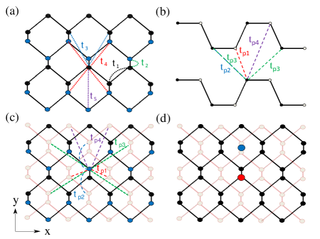
Figure 1: Lattice structure of single-layer and bilayer BP. The relevant hopping terms considered in the Hamiltonian (1) are shown. The red and blue dots in (d) represent a resonant scatterer and a Gaussian center, respectively.

II Model and Method

BP is a single-elemental layered crystalline material consisting of only phosphorus atoms arranged in a puckered orthorhombic lattice. As sketched in Fig. 1, single layer phosphorene contains two atomic layers and two kinds of bonds with 2.22 Å  and 2.24 Å  bond lengths for in-plane and inter-plane P-P connections, respectively.Morita (1986) The electronic band structure around the gap can be described with a TB Hamiltonian for pristine BP with the formRudenko and Katsnelson (2014)

$$\mathcal{H}=\sum_{i}\epsilon_{i}n_{i}+\sum_{i\neq j}t_{ij}c_{i}^{\dagger}c_{j}+\sum_{i\neq j}t_{p,ij}c_{i}^{\dagger}c_{j},$$ (1)

where we consider five intralayer ($t_{1}=-1.220$ eV, $t_{2}=3.665$ eV, $t_{3}=-0.205$ eV, $t_{4}=-0.105$ eV, $t_{5}=-0.055$ eV) and four interlayer hopping terms ($t_{p1}=0.295$ eV, $t_{p2}=0.273$ eV, $t_{p3}=-0.151$ eV, $t_{p4}=-0.091$ eV). For unbiased bilayer BP, there is an energy splitting of $\Delta\epsilon=1.0$ eV between the nonequivalent electrons in the sublayers. This model, which is based on first principle $GW$ calculations, accurately reproduces the conduction and valence bands for energies $\sim$0.3 eV beyond the gap. For a detailed description of the above TB Hamiltonian we refer the reader to Ref. Rudenko and Katsnelson, 2014.

We consider two main different sources of disorder in BP: local point defects and long range disorder potential. Point defects are modeled by elimination of atoms randomly over the whole sample, which can be viewed as vacancies, chemical adsorbates or substitution of other types of atoms which prevent the hopping of electrons to their neighbor sites.Neto et al. (2009); Das Sarma et al. (2011); Katsnelson (2012); Yuan et al. (2010a, b); Qiu et al. (2013); Yuan et al. (2014, 2015) This type of point defects are the so called resonant scatterers which provide resonances within the band gap Yuan et al. (2014); Qiu et al. (2013); Yuan et al. (2015), as confirmed by first-principles calculations which include single vacanciesLiu et al. (2014b); Hu and Yang (2014), adatoms (Si, Ge, Au, Ti, V)Kulish et al. (2015), absorption of organic moleculesZhang et al. (2014), substitutional p-dopants (Te, C)Liu et al. (2014b) or oxygen bridge-type defectsZiletti et al. (2015).

The long-range disorder potential (LRDP), on the other hand, can account for electron-hole puddles, which are random changes of the local potential due to the inhomogeneous distribution of charge in the sample. Within the TB model, it can be considered as a correlated Gaussian potential,Lewenkopf et al. (2008); Yuan et al. (2010b, 2011b) such that the potential at site $i$ follows

$$v_{i}=\sum_{k}U_{k}\exp\left(-\frac{\left|\mathbf{r}_{i}-\mathbf{r}_{k}\right|^{2}}{2d^{2}}\right),$$ (2)

where $\mathbf{r}_{k}$ is the position of the $k$-th Gaussian center, which are chosen to be randomly distributed over the centers of the projected lattice on the surface, $U_{k}$ is the amplitude of the potential at the $k$-th Gaussian center, which is uniformly random in the range $[-\Delta,\Delta]$, and $d$ is interpreted as the effective potential radius. Typical values of $\Delta$ and $d$ used in our model are $\Delta=5$ eV and $d=5a$ for LRDP.Yuan et al. (2010b, 2011b, 2015) Here $a\approx 2.216$Å is the atomic distance of two nearest neighbors within the same plane. The origin of LRDP could be screened charged impurities on the substrate Hwang et al. (2007); Zhang et al. (2009); Rudenko et al. (2011); Principi et al. (2013) or surface corrugations such as ripples and wrinklesGibertini et al. (2010, 2012). Although LRDP does not introduce resonances in the spectrum, they lead to an uniform increase of states in the gap.Yuan et al. (2015) The amount of resonant scatterers and Gaussian centers are quantified by $n_{x}$ and $n_{c}$, respectively, which are the probability for a scatterer or Gaussian center to exist.

The excitation spectrum and screening of single- and bilayer BP are calculated by using the TBPM.Yuan et al. (2010a, 2011a, 2012) The dynamic polarization function is obtained from the Kubo formula Kubo (1957)

$$\Pi\left(\mathbf{q},\omega\right)=\frac{i}{V}\int_{0}^{\infty}d\tau e^{i\omega\tau}\left\langle\left[\rho\left(\mathbf{q},\tau\right),\rho\left(-\mathbf{q},0\right)\right]\right\rangle,$$ (3)

where $V$ denotes the volume (or area in 2D) of the unit cell, $\rho\left(\mathbf{q}\right)$ is the density operator given by

$$\rho\left(\mathbf{q}\right)=\sum_{l=1}^{N_{layer}}\sum_{i}c_{l,i}^{\dagger}c_{l,i}\exp\left(i\mathbf{q\cdot r}_{l,i}\right),$$ (4)

and the average in (3) is taken over the canonical ensemble. For the case of the single-particle Hamiltonian, Eq. (3) can be written asYuan et al. (2011a)

$$\Pi\left(\mathbf{q},\omega\right)=-\frac{2}{V}\int_{0}^{\infty}d\tau e^{i\omega\tau}$$

$$\times\mathrm{Im}\left\langle\varphi\right|n_{F}\left(H\right)e^{iH\tau}\rho\left(\mathbf{q}\right)e^{-iH\tau}\left[1-n_{F}\left(H\right)\right]\rho\left(-\mathbf{q}\right)\left|\varphi\right\rangle,$$

where $n_{F}\left(H\right)=\frac{1}{e^{\beta\left(H-\mu\right)}+1}$ is the Fermi-Dirac distribution operator, $\beta=1/k_{B}T$ where $k_{B}$ is the Boltzmann constant and $T$ is the temperature, and $\mu$ is the chemical potential. We use units such that $\hbar=1$ and the average in Eq. (II) is performed over a random phase superposition of all the basis states in the real space, i.e.,Hams and De Raedt (2000); Yuan et al. (2010a)

$$\left|\varphi\right\rangle=\sum_{l,i}a_{l,i}c_{l,i}^{\dagger}\left|0\right\rangle,$$ (6)

where the coefficients $a_{l,i}$ are random complex numbers normalized as $\sum_{l,i}\left|a_{l,i}\right|^{2}=1$. We next introduce the time evolution of two wave functions

$$\left|\varphi_{1}\left(\mathbf{q,}\tau\right)\right\rangle = e^{-iH\tau}\left[1-n_{F}\left(H\right)\right]\rho\left(-\mathbf{q}\right)\left|\varphi\right\rangle,$$ (7)

$$\left|\varphi_{2}\left(\tau\right)\right\rangle = e^{-iH\tau}n_{F}\left(H\right)\left|\varphi\right\rangle,$$ (8)

which allows us to express the real and imaginary part of the dynamic polarization as

$$\mathrm{Re}\Pi\left(\mathbf{q},\omega\right) = -\frac{2}{V}\int_{0}^{\infty}d\tau\cos(\omega\tau)\leavevmode\nobreak\ \text{Im}\left\langle\varphi_{2}\left(\tau\right)\left|\rho\left(\mathbf{q}\right)\right|\varphi_{1}\left(\tau\right)\right\rangle,$$

$$\mathrm{Im}\Pi\left(\mathbf{q},\omega\right) = -\frac{2}{V}\int_{0}^{\infty}d\tau\sin(\omega\tau)\leavevmode\nobreak\ \text{Im}\left\langle\varphi_{2}\left(\tau\right)\left|\rho\left(\mathbf{q}\right)\right|\varphi_{1}\left(\tau\right)\right\rangle.$$

The time evolution operator $e^{-iH\tau}$ and Fermi-Dirac distribution operator $n_{F}\left(H\right)$ can be obtained from the standard Chebyshev polynomial decomposition.Yuan et al. (2010a) In our calculations, the chemical potential is set to be $\sim 0.1$ eV above the edge of conduction band, i.e., $\mu=0.4$ eV for single-layer and $0.73$ eV for bilayer BP. The temperature is fixed at $T=300$ K. We use periodic boundary conditions, and the system size is $8192\times 8192$ for single-layer BP, and $6000\times 6000$ for bilayer.

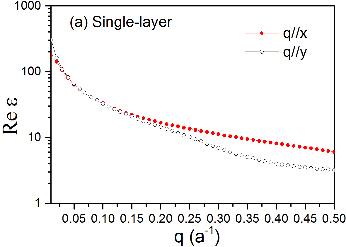
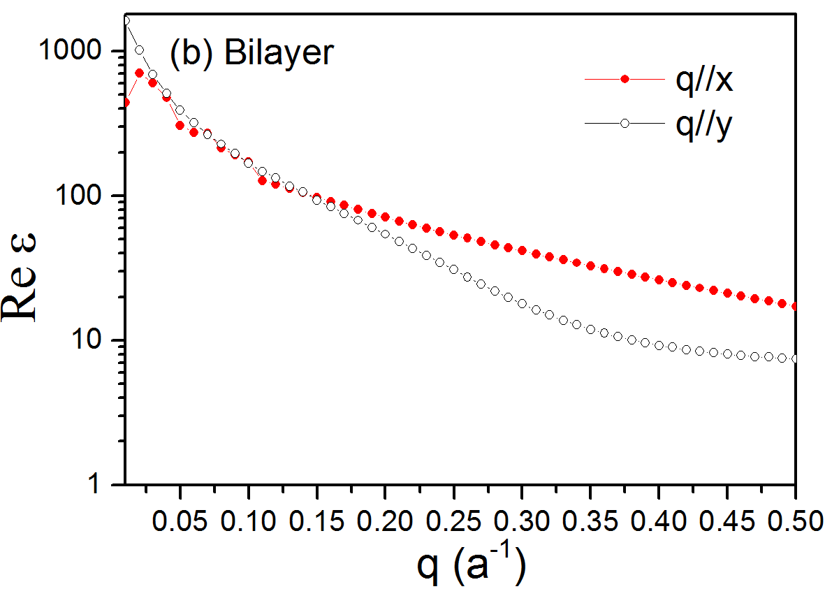
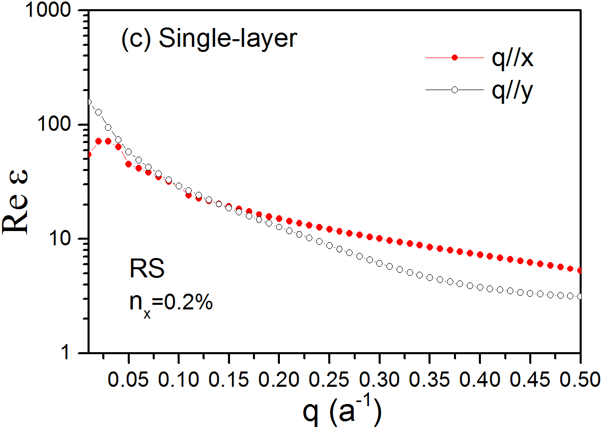
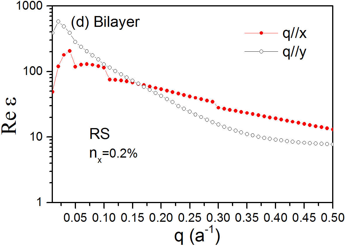
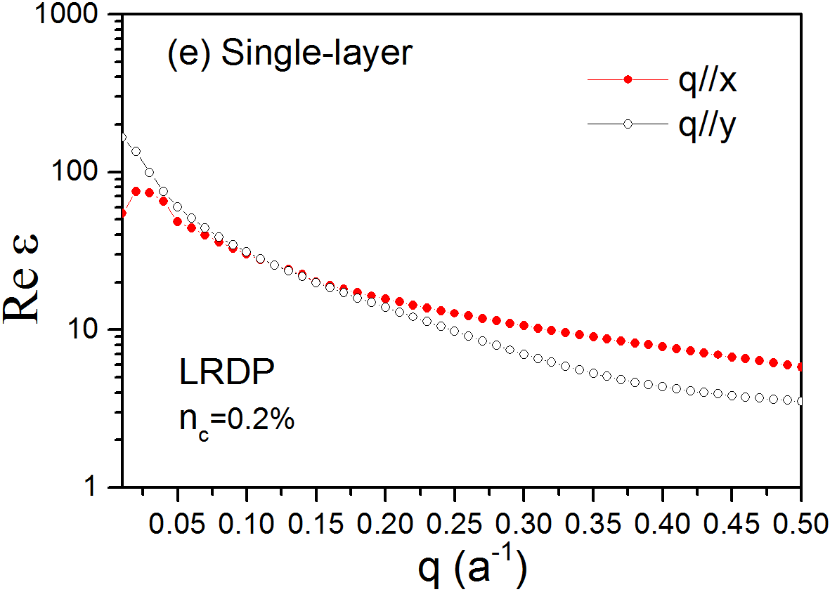
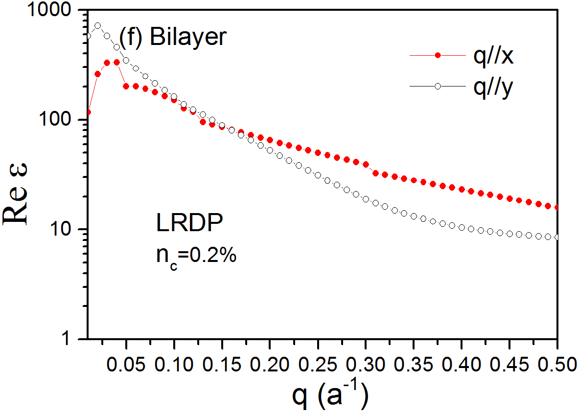
Figure 2: Static dielectric function of single- (left) and bilayer (right) BP. The chemical potential is set to be $\mu=0.4$ eV for single-layer and $0.73$ eV for bilayer. The temperature is fixed as the room tempertuare $T=300$ K. Plots (a) and (b) correspond to pristine BP, (c) and (d) correspond to samples with resonant scatterers originated from a concentration of $n_{x}=0.2\%$ vacant atoms, and (e) and (f) correspond to samples with long range disorder potential with a concentration of $n_{c}=0.2\%$ Gaussian centers.

Electron-electron interactions are considered within the RPA. The two-dimensional dielectric function for single-layer phosphorene is calculated as

$$\mathbf{\varepsilon}_{1L}\left(\mathbf{q},\omega\right)=\mathbf{1}-V\left(q\right)\Pi\left(\mathbf{q},\omega\right)$$ (10)

where

$$V\left(q\right)=\frac{2\pi e^{2}}{\kappa q}$$ (11)

is the Fourier component of the Coulomb interaction in two dimensions, in terms of the background dielectric constant $\kappa$. For bilayer BP, the Coulomb interaction has a matrix form

$${\tilde{\mathbf{V}}}(q)=\left(\begin{array}[]{cc}V_{\mathrm{intra}}(q)&V_{\mathrm{inter}}(q)\\ V_{\mathrm{inter}}(q)&V_{\mathrm{intra}}(q)\end{array}\right),$$

where $V_{\mathrm{intra}}(q)=V(q)$ as given by Eq. (11), and the interlayer interaction between electrons in different BP layers is $V_{\mathrm{inter}}=F(q)V(q)$ where $F(q)=e^{-qd}$ and $d=0.5455$ nm is the interlayer distance. From this we can express the dielectric tensor for bilayer BP, including the intralayer and interlayer contributions, as

$$\mathbf{\varepsilon}_{2L}\left(\mathbf{q},\omega\right)$$ (14)

$$= \left(\begin{array}[]{cc}\mathbf{\varepsilon}_{1L}\left(\mathbf{q},\omega\right)&-V\left(q\right)F\left(q\right)\Pi\left(\mathbf{q},\omega\right)\\ -V\left(q\right)F\left(q\right)\Pi\left(\mathbf{q},\omega\right)&\mathbf{\varepsilon}_{1L}\left(\mathbf{q},\omega\right)\end{array}\right).$$

In the next sections we use the polarization and dielectric functions defined here to study the effect of disorder on the screening properties and the collective plasmon modes of BP. To simplify the notation, we use $\mathbf{\ \varepsilon}\left(\mathbf{q},\omega\right)$ to represent $\mathbf{\varepsilon}_{1L}\left(\mathbf{q},\omega\right)$ for single-layer and the determinant of the dielectric tensor $\left|\mathbf{\varepsilon}_{2L}\left(\mathbf{q},\omega\right)\right|$ for bilayer.

III Dielectric screening

We start by studying the effect of disorder on the screening properties. In Fig. 2, we plot the static dielectric function $\mathbf{\varepsilon}\left(\mathbf{q},0\right)$ of single- and bilayer BP. There is a clear dependence of the static dielectric function with the direction of momentum, showing a different behavior for $\mathbf{q}$ along the zigzag (X) or armchair (Y) directions. For the pristine case, our numerical results for the momentum dependence of the static dielectric function of single-layer phosphorene, Fig. 2(a), agree with the analytic low energy model presented in Ref. Low et al., 2014c. The present calculation within the TBPM method allows us to extend the calculation of Ref. Low et al., 2014c to larger wave-vectors and to consider realistic impurities in the sample. We notice that the size of the lattices used in our simulations determines the rage of wave-vectors for our numerical results, which is $q\geq 0.01a^{-1}$. We do not perform calculations with momentum transfer smaller than $q=0.01a^{-1}$ since, in order to preserve the numerical accuracy for $q\rightarrow 0$, an extreamly large sample size $N\rightarrow\infty$ is required.

In both single- and bilayer BP, point-like resonant scatterers lead to the creation of midgap states inside the gap.Yuan et al. (2015) These states are quasi-localized around the center of the impurity. Therefore, the typical divergence of the dielectric function at $q\rightarrow 0$, characteristic of metallic behavior, is reduced for BP crystals with this kind of disorder, as it can be seen in Fig. 2(c)-(d). A similar result for the dielectric function is obtained for LRDP which can be associated to the existence of electron-hole puddles in the sample. A drop of the dielectric function at small $q$ appears also in disordered graphene with chemical absorbers. Yuan et al. (2012) The effect of disorder on the static dielectric function is negligible at short wave-lengths (large $q$ vectors).

IV Energy Loss Function and Plasmons

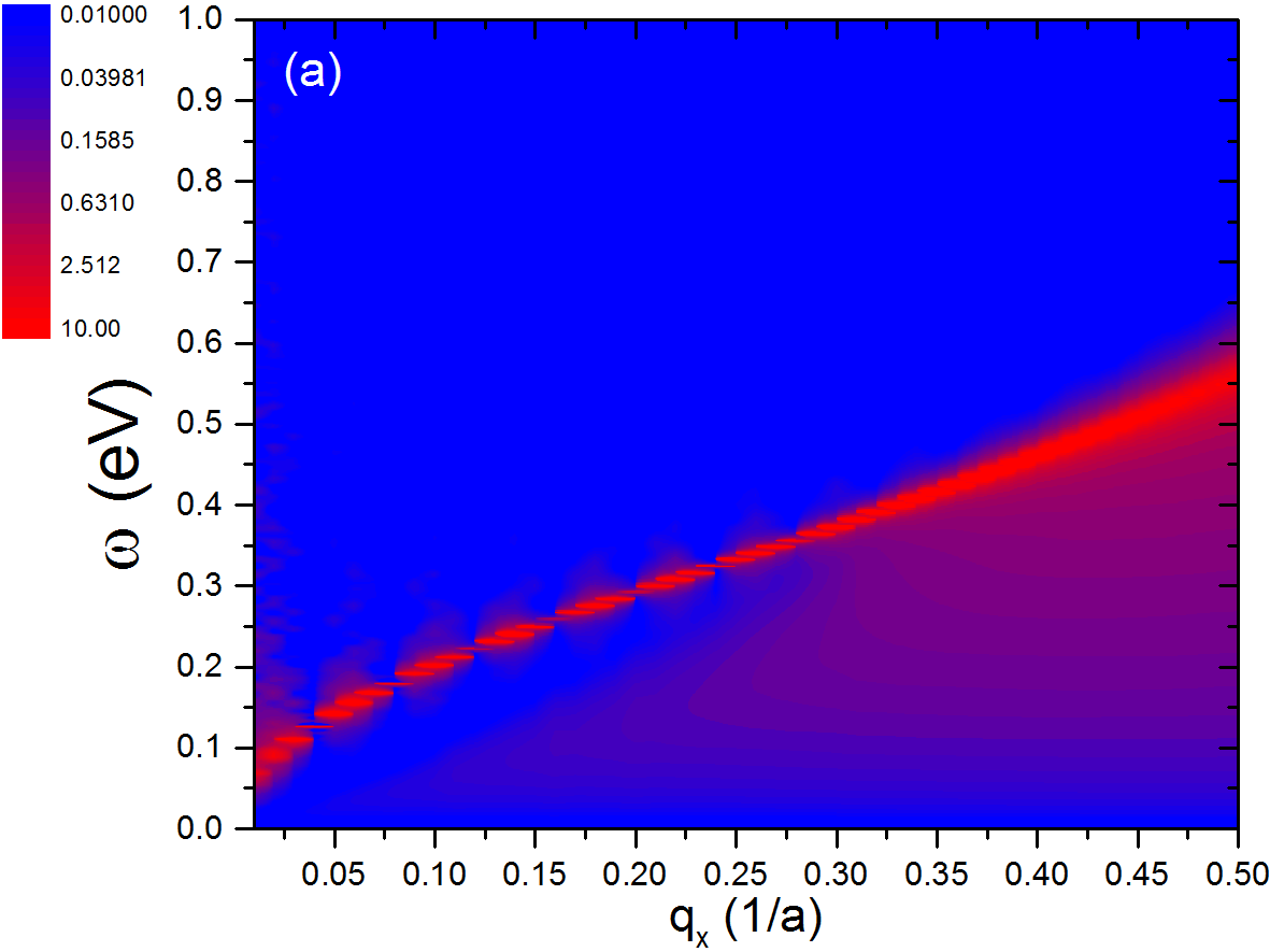
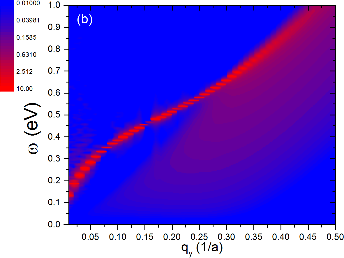
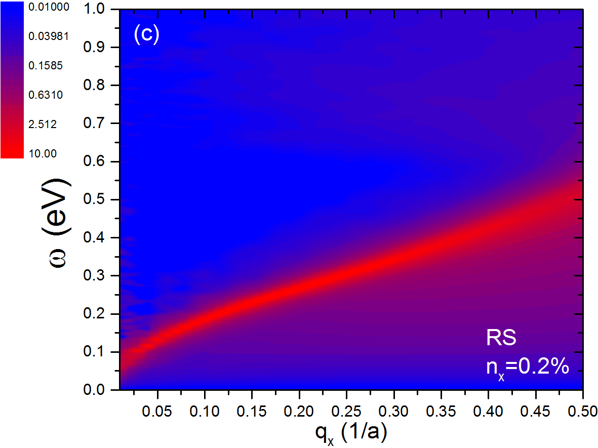
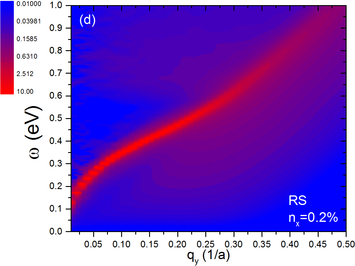
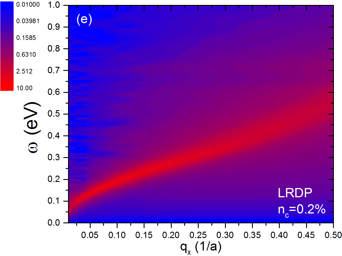
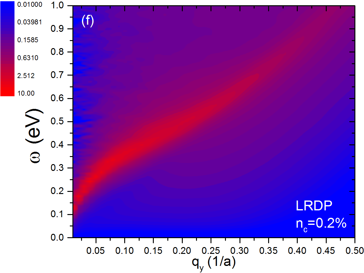
Figure 3: Energy loss functions of single-layer BP along zigzag (left) and armchair (right) directions. The simulations are done for: (a,b) pristine BP, (c,d) samples with resonant scatterers, and (e,f) samples with long-range disorder potentials. All the results are calculated at $T=300$ K. We notice that the apparent discretization of the spectrum in some of the plots is an artifact due to finite size limitations in our calculations.

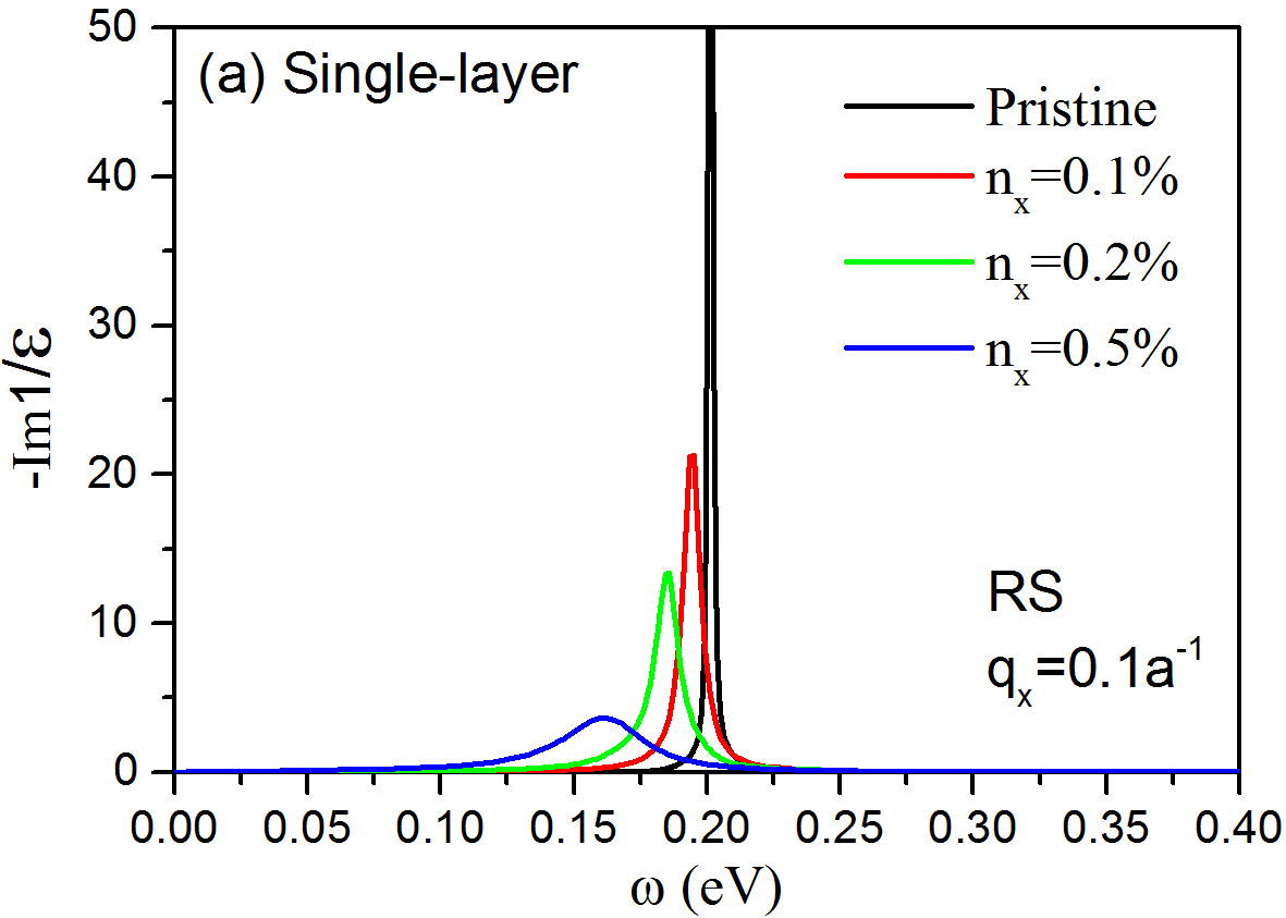
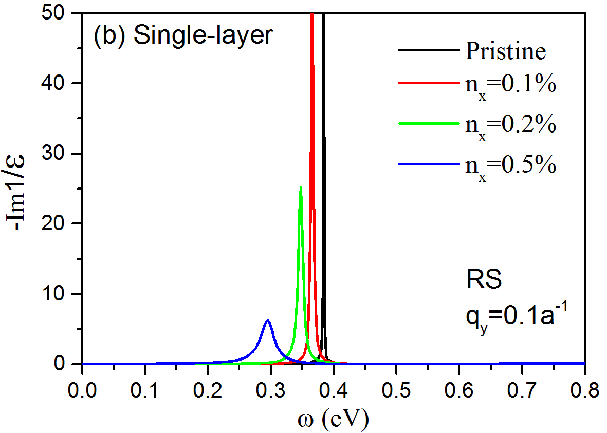
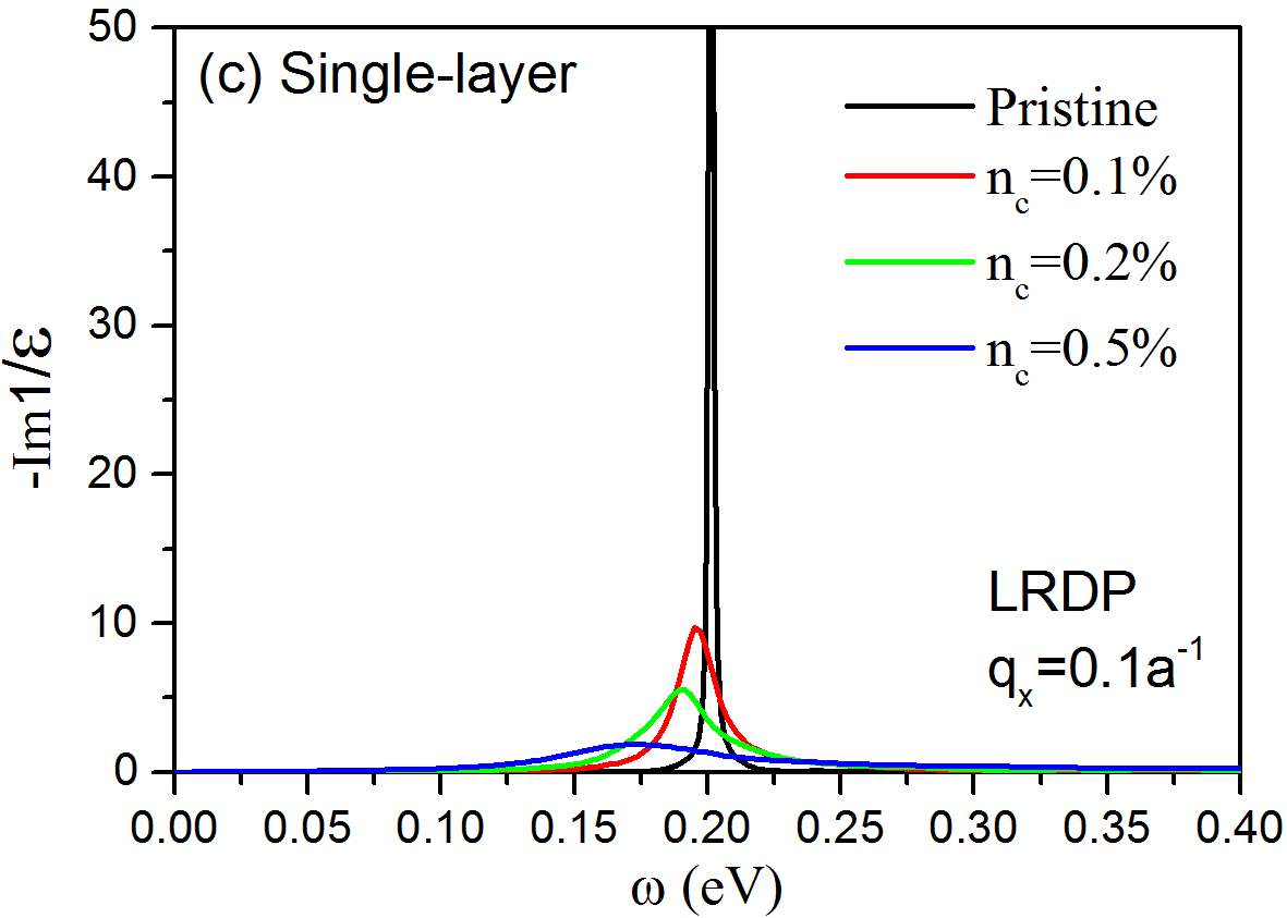
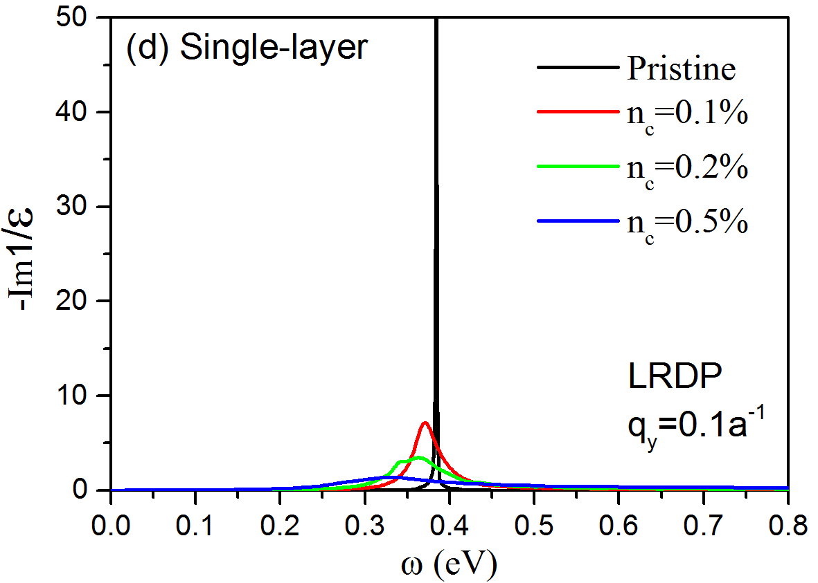
Figure 4: Energy loss functions of single-layer BP along zigzag (left) and armchair (right) directions. Panels (a) and (b) compare the loss function of pristine single-layer BP with that of samples with different concentrations of point defects. Panels (c) and (d) correspond to LRDP. All the results are calculated at $T=300$ K.

In this section we study the collective modes of the system, which are defined by the zeroes of the dielectric function $\mathbf{\varepsilon}\left(\mathbf{q},\omega\right)$ for single-layer BP (or zeroes of the dielectric tensor determinant for bilayer BP). The dispersion relation of the plasmon modes is defined from $\mathrm{Re}\leavevmode\nobreak\ \varepsilon(\mathbf{q},\omega_{pl})=0,$ which leads to poles in the energy loss function $-\Im 1/\varepsilon(q,\omega)$, that can be measured by means of electron energy loss spectroscopy (EELS).Politano and Chiarello (2014)

IV.1 Single-layer BP

For single-layer BP, our numerical results for the loss function are plotted in Fig. 3 and show anisotropic plasmon modes along the zigzag and armchair directions, both following a low energy $\sqrt{q}$ dependence at small momentum transfer. This is due to the paraboloidal band dispersion of BP at low energies, and it is consistent with the results for the excitation spectrum of BP within the $\mathbf{k\cdot p}$ approximation.Low et al. (2014c) The present method allows us to study the spectrum at higher energies and wave-vectors, including also the effect of disorder in the sample.

In the presence of disorder, there is a broadening and red shift of the plasmon modes, as it can be seen in Fig. 3(c)-(d) for single-layer samples with resonant scatterers, and in Fig. 3(e)-(f) for long range disorder potential. For a fixed wave-vector, the effect of disorder is better seen by the loss function shown in Fig. 4 for $q=0.1a^{-1}$ and different concentrations of disorder. Notice that the presence of LRPD induces a stronger damping of the plasmon, as compared to point defects. This is seen by comparing the broadening of the peaks of the top and bottom panels of Fig. 4. Since plasmons are collective electronic oscillations induced by long range Coulomb interaction, it is expected that long range disorder affects more the coherence of these modes than local scatterers as vacancies, which are relevant at short length scales.

Fig. 4 also shows that, for a given wavelength, the two kinds of disorder considered in our simulations lead to a shift of the plasmon resonance towards lower energies. This effect can be understood from a perturbative point of view, by using the disordered averaged response function introduced by Mermin in the context of a 2DEG with a parabolic band dispersion,Mermin (1970) and which has been recently used to study the effect of weak disorder on the plasmon dispersion of spin-polarized graphene.Agarwal and Vignale (2015) In the weak disorder limit, and assuming for simplicity an isotropic parabolic band dispersion, the disordered averaged response function has the formMermin (1970); Giuliani and Vignale (2005)

$$\Pi_{imp}(\mathbf{q},\omega)\approx-N(0)\left(1-\frac{\omega}{\sqrt{(\omega+i/\tau_{el})^{2}-v_{F}^{2}q^{2}}-i/\tau_{el}}\right)$$ (16)

where $\tau_{el}$ is the elastic life-time of the momentum eigenstates of the disordered system, $N(0)=gm_{b}/2\pi$ is the density of states (per unit area) at the Fermi energy, where $g=2$ is the spin degeneracy, $m_{b}$ is the effective mass, and $v_{F}$ is the Fermi velocity. In the presence of disorder the dispersion relation of the plasmon will have, even in the low energy and long wavelength limit, and imaginary part, due to finite damping of the plasmon. Within this approximation, it is possible to obtain an analytical expression for the plasmon dispersion by substituting (16) into (10) and then finding the zeros of the dielectric function, with the approximate solution

$$\omega_{pl}(q)\approx\frac{q+4r_{s}k_{F}}{q+8r_{s}k_{F}}\left(\sqrt{v_{F}^{2}q(q+8r_{s}k_{F})-1/\tau_{el}^{2}}-i/\tau_{el}\right)$$ (17)

where $r_{s}=2m_{b}e^{2}/\kappa k_{F}$ is the dimensionless interaction parameter of a 2DEG and $k_{F}$ is the Fermi wave-vector. Eq. (17) reduces to the standard plasmon dispersion in the clean ($1/\tau_{el}\rightarrow 0$) limit. We notice here that the presence of impurities limit the dispersion of collective plasmon modes for length scales longer than the mean free path, defining a minimal wave-vector below which the plasmon mode is not well defined. The existence of such length scale has been discussed, in the context of graphene, in Ref. Agarwal and Vignale, 2015. For the case of interest here such infrared cutoff takes the form $q_{min}=-4r_{s}k_{F}+\sqrt{8r_{s}^{2}k_{F}^{2}+1/\tau_{el}^{2}v_{F}^{2}}$, below which plasmon modes do not exist.

The next step in our analysis is to quantify the effect of disorder on plasmon losses. The physical observability of a damped collective mode depends on the sharpness of the resonance peak, and it is defined as a dimensionless inverse quality factor $\mathcal{R}=\gamma/\omega_{pl}$, where the damping rate $\gamma$ of the mode, which is proportional to $\mathrm{Im}\leavevmode\nobreak\ \Pi(\mathbf{q},\omega_{pl})$, is given by

$$\gamma=\frac{\mathrm{Im}\leavevmode\nobreak\ \Pi(\mathbf{q},\omega_{pl})}{\left.\frac{\partial}{\partial\omega}\mathrm{Re}\leavevmode\nobreak\ \Pi(\mathbf{q},\omega)\right|_{\omega=\omega_{pl}}}.$$ (18)

The plasmon lifetime $\tau$ is calculated via the inverse quality factor as $\tau=1/\mathcal{R}\omega_{pl}.$ We have calculated numerically $\mathcal{R}$ ($\gamma$) and $\tau$, and the results are shown in Fig. 5. We first notice that, for a given concentration of impurities and for a given wavelength, the plasmon rate is anisotropic. In fact, our results show that plasmons dispersing in the $y$-direction (armchair) are more efficiently damped than plasmons dispersing in the $x$ (zigzag) direction, which have a larger lifetime. Second, as discussed above, we find that short range resonant scatterers like point defects cause less losses in the plasmon coherence than LRDP.

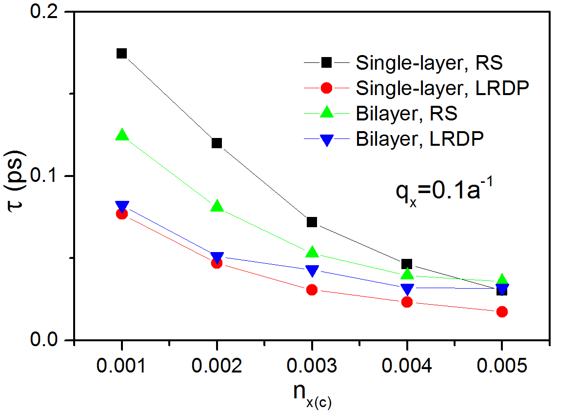
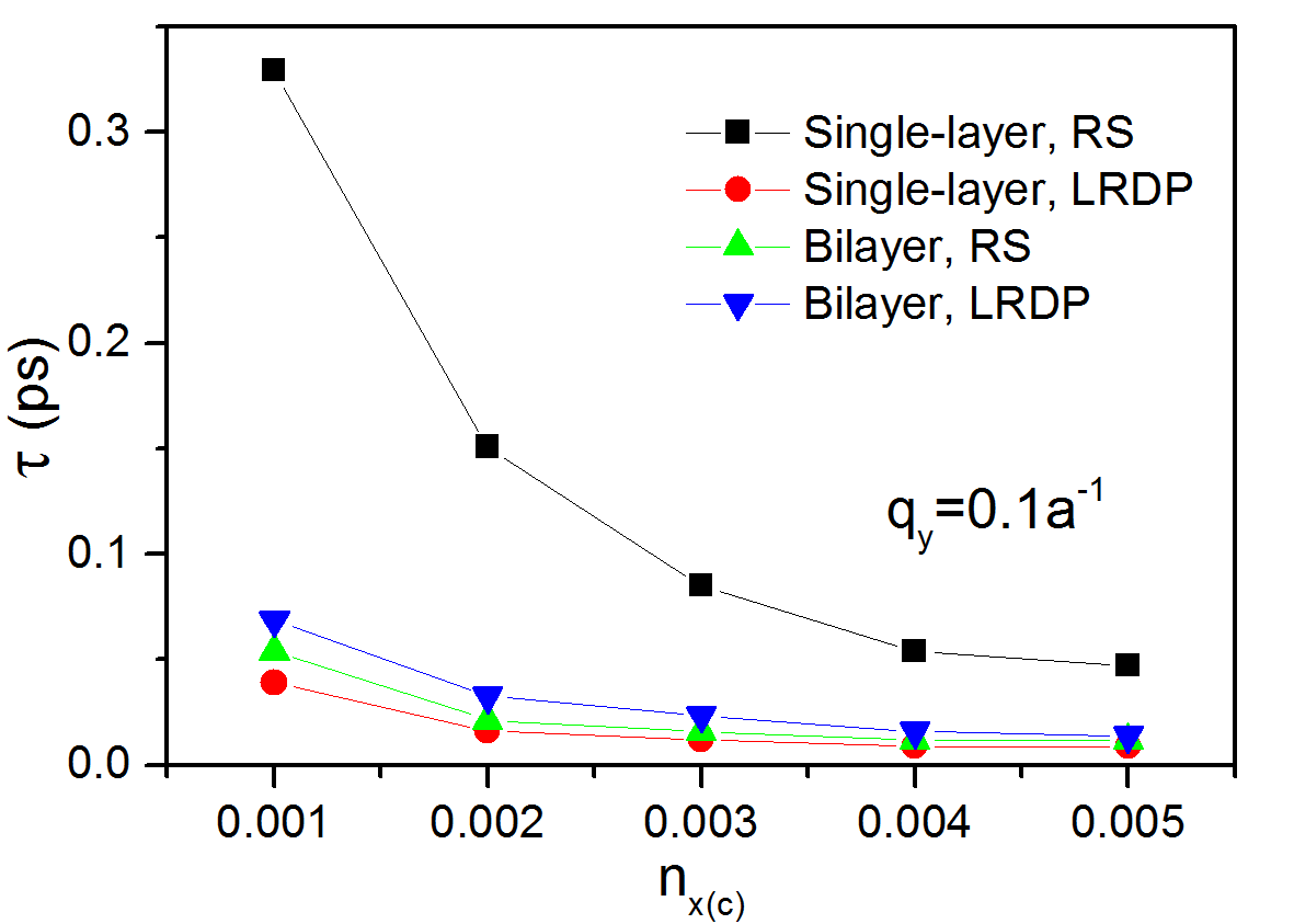
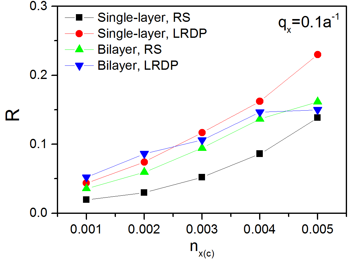
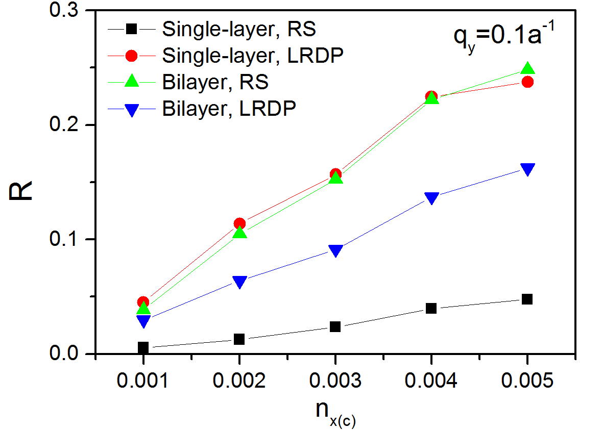
Figure 5: Effect of disorder on plasmon losses. Panels (a) and (b) show the plasmon life-time, and panels (c) and (d) show the corresponding damping rates (inverse quality factor). The results for bilayer BP samples correspond to the in-phase $\sim\sqrt{q}$ plasmon mode (see text).

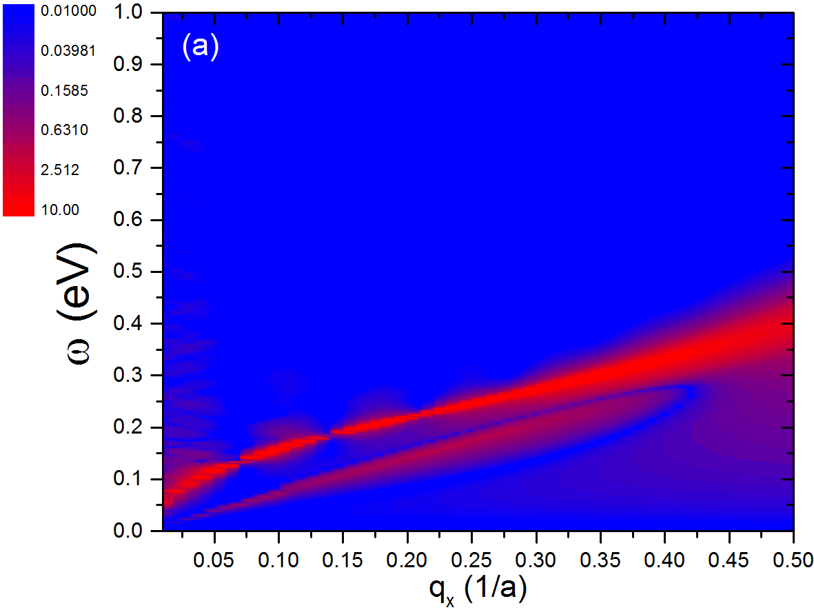
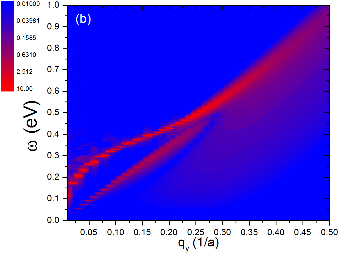
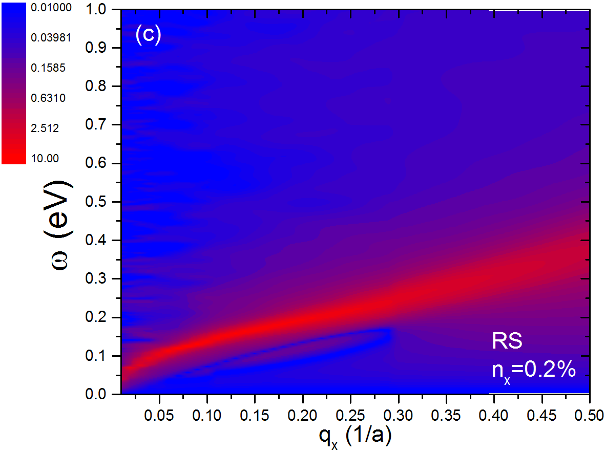
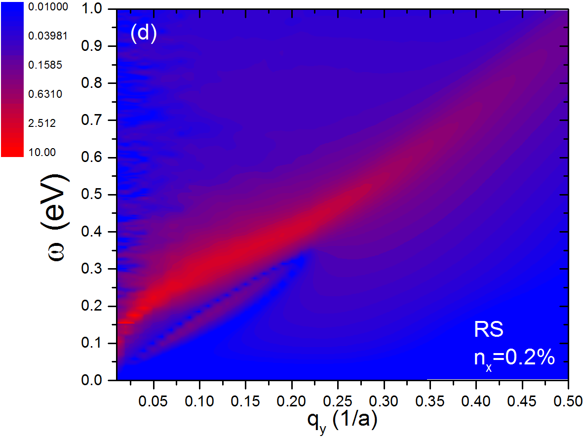
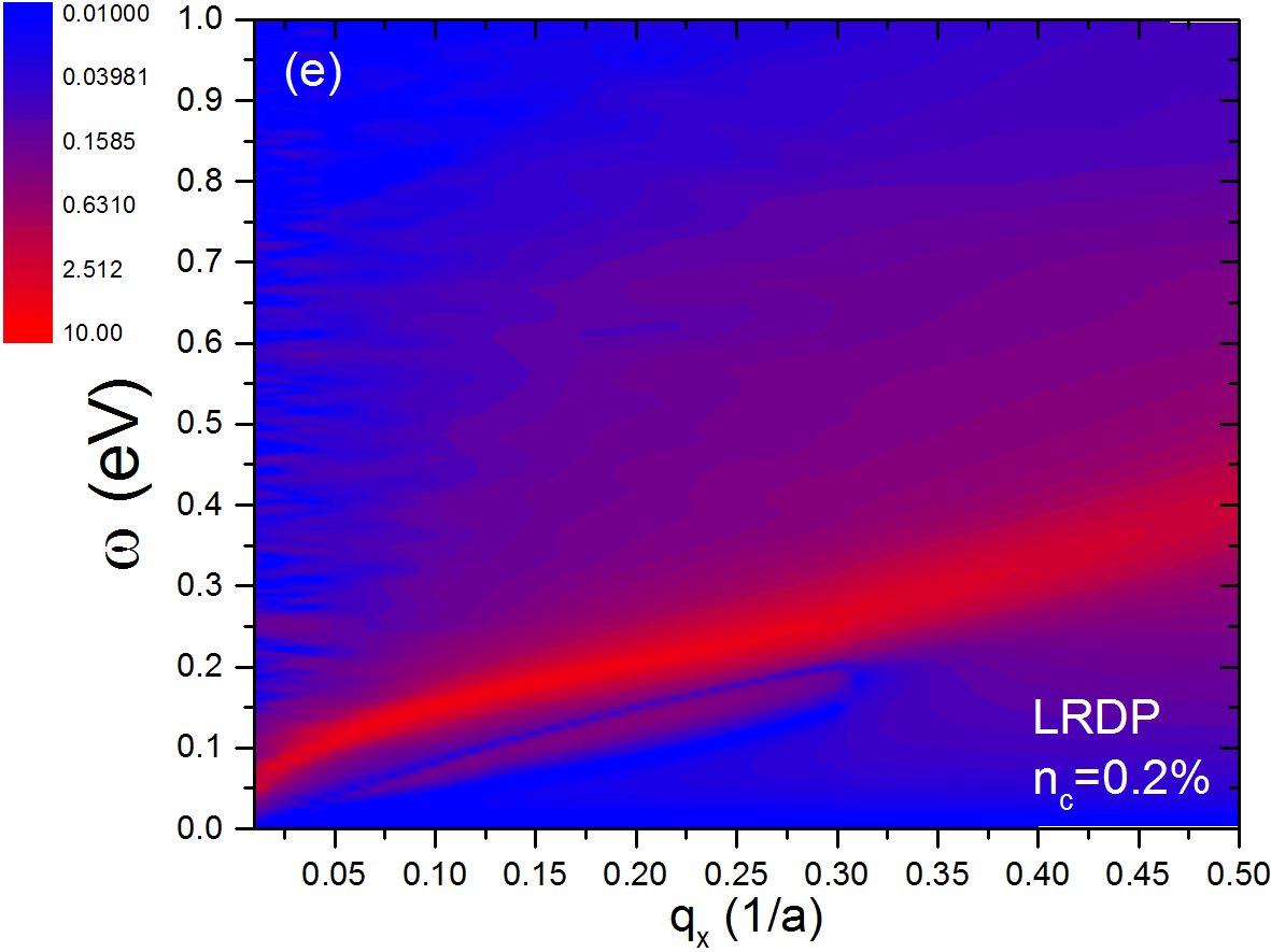
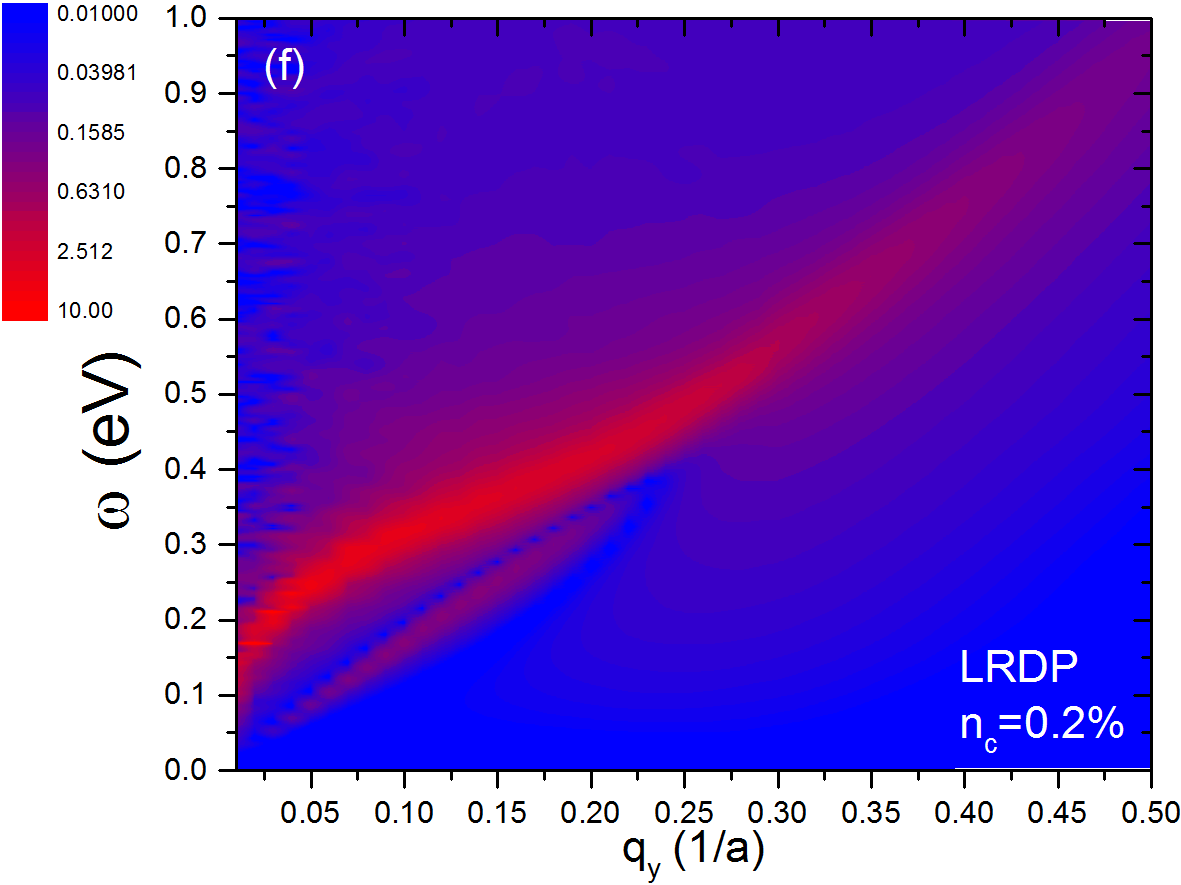
Figure 6: Energy loss functions of bilayer BP along zigzag (left) and armchair (right) directions. The simulations are done for: (a,b) pristine bilayer BP, (c,d) samples with resonant scatterers, and (e,f) samples with long-range disorder potentials. All the results are calculated at $T=300$ K.

IV.2 Bilayer BP

In the following we present results for bilayer BP, considered as two phosphorene layers coupled by interlayer hopping (see Fig. 1), and interacting via long range Coulomb potential, as explained in Sec. II. Our results for the loss function are shown in Fig. 6. The first thing to notice is the existence of two collective modes in the spectrum, as it is usual in bilayer systems.Das Sarma and Hwang (1998); Gamayun (2011); Roldán and Brey (2013); Rodin and Castro Neto (2015) One is the classical $\omega_{+}(q\rightarrow 0)\sim\sqrt{q}$ plasmon mode, which has its counterpart in single-layer samples (see Fig. 3). This mode correspond to a collective excitation of the electron liquid in which the carriers of both layers oscillate in-phase. In addition to this plasmon, in Fig. 6 we observe the existence of an additional mode in the excitation spectrum dispersing below the $\omega_{+}$ plasmon. This mode, with a low energy linear dispersion relation, $\omega_{-}(q\rightarrow 0)\sim q$, is characteristic of bilayer 2DEG systems and corresponds to a collective oscillation in which the carrier density in the two layers oscillates out-of-phase. The existence of this mode is also clear in Fig. 7, where it can be seen that, besides the peak in the loss function corresponding to the in-phase $\omega_{+}$ plasmon, there is a second resonance at lower energies (with less spectral weight) which corresponds to the $\omega_{-}\sim q$ plasmon (indicated by black arrows). The $\omega_{-}$ mode is much weaker as compared to the $\omega_{+}$ mode because of the short distance between the two layers, which complicates the out-of-phase density oscillation. In Ref. Rodin and Castro Neto, 2015, the two modes discussed above have been also obtained by using a general low energy model of anisotropic double-layer systems. We notice here that, since they study bilayer systems in which the two layers are separated by more than 5 nm,Rodin and Castro Neto (2015) their results show a $\omega_{-}$ mode that is more coherent and dispersing than the one obtained in our calculations. As a matter of fact, the dispersion relation of the out-of-phase mode is proportional to the layer separation, $\omega_{-}(q)\sim d^{1/2}q$, where $d$ is the interlayer distance. Here we restrict our study to real bilayer phosphorene, in which the two layers are separated by $d=0.524$ nm, and interlayer hopping of electrons is allowed. As a consequence, the $\omega_{-}$ mode obtained in our simulations for bilayer BP disperses with a smaller velocity than the mode of Ref. Rodin and Castro Neto, 2015.

We also observe that, as in the single-layer case, both modes are damped due to disorder. The characteristics of the damping of the in-phase $\omega_{+}\sim\sqrt{q}$ mode can be understood from the previous analysis for single-layer BP. Losses are stronger in the out-of-phase $\omega_{-}$ plasmon, whose coherence basically vanishes due to disorder. The reasons for this are twofold. On the one hand, the spectral weight of the $\omega_{-}$ mode is considerably weaker than the $\omega_{+}$ plasmon. On the other hand, the $\omega_{-}$ mode disperses in the $\omega-q$ spectrum very close to the electron-hole continuum, whose threshold can be reached due to disorder (and thermal) broadening of the plasmon peak, with the consequent Landau damping of the mode.

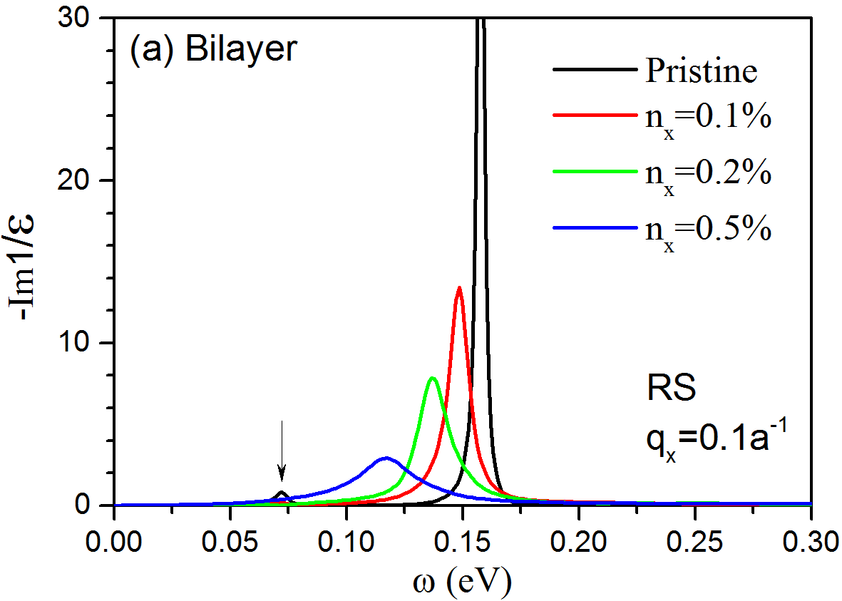
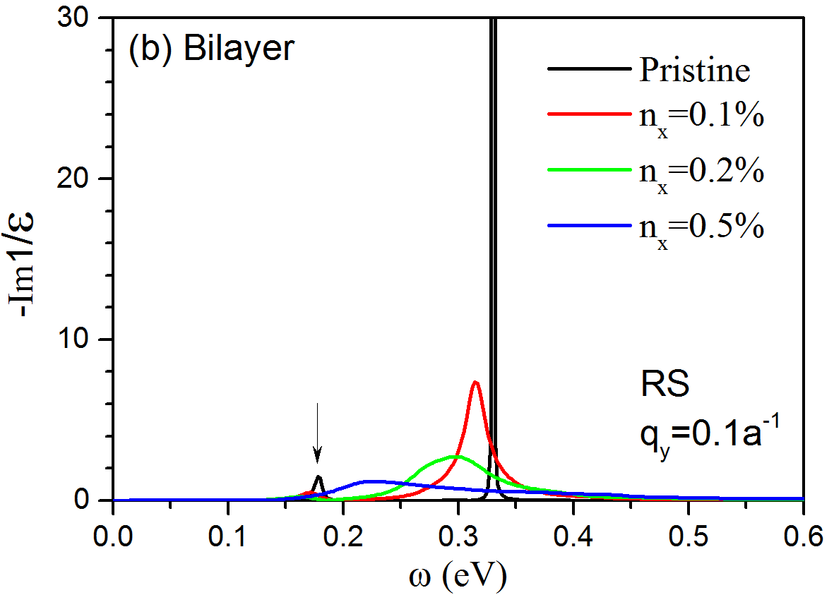
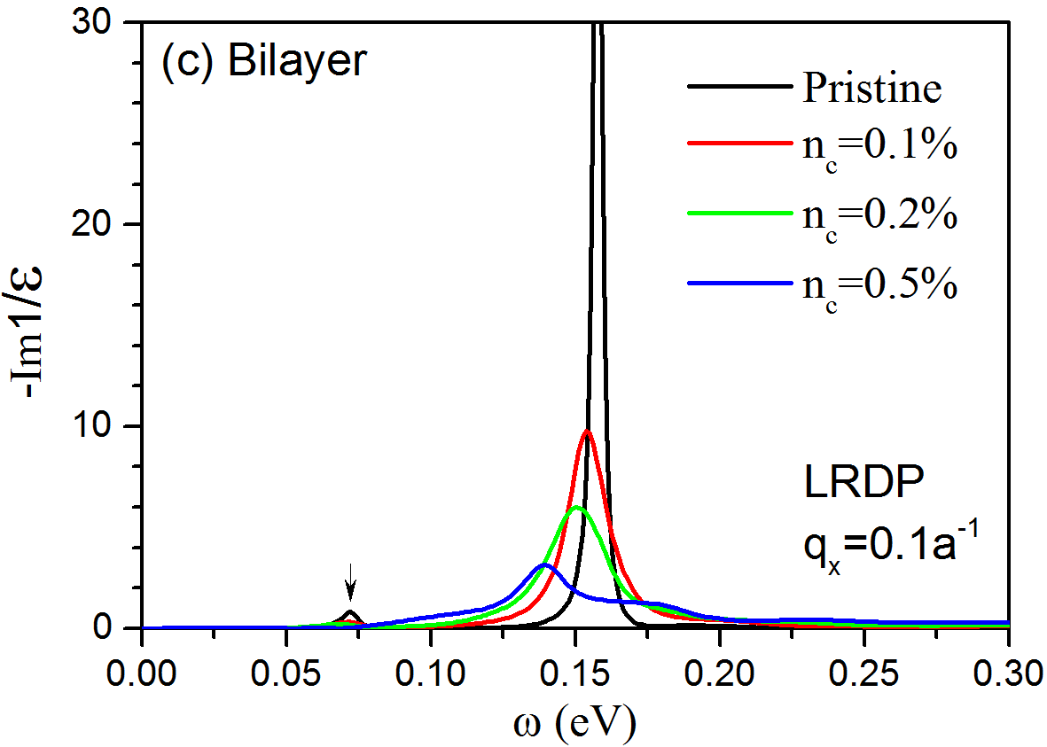
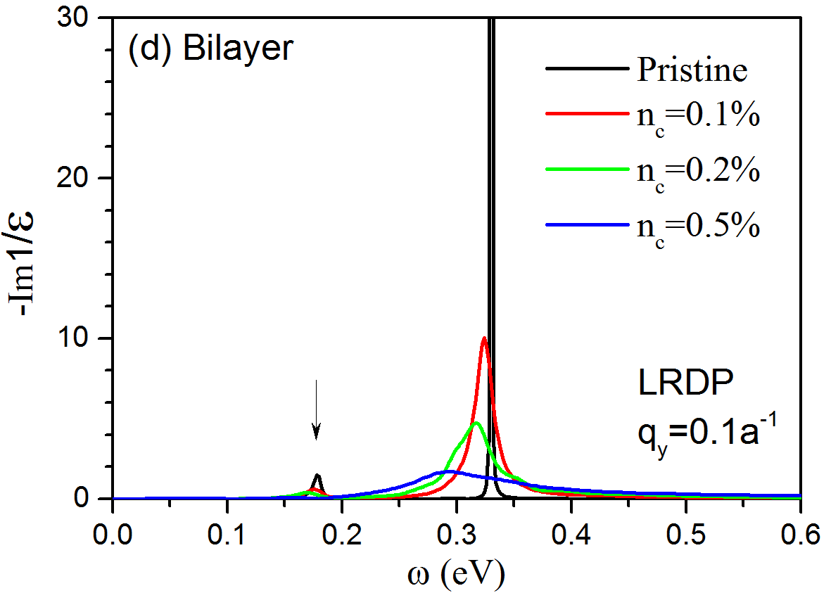
Figure 7: Energy loss functions of bilayer BP along zigzag (left) and armchair (right) directions. Panels (a) and (b) compare the loss function of pristine bilayer BP with that of samples with different concentrations of point defects. Panels (c) and (d) correspond to LRDP. All the results are calculated at $T=300$ K. The peak marked by arrows in each panel correspond to the out-of-phase $\omega_{-}(q)\sim q$ plasmon (see text).

IV.3 Biased Bilayer BP

In this section we include in our calculations the presence of a perpendicular electric field applied to the bilayer BP. This technique can be used to manipulate the electronic band structure of the system, and it has been proposed recently as an appropriate way to drive a normal to topological phase in this material.Liu et al. (2015); Dolui and Quek (2015) Here we are interested on studying the effect of an electric field on the dispersion relation of plasmons. For this aim, we introduce a biased on-site potential difference $\Delta$ between the two layers as described in Ref. Pereira and Katsnelson, 2015, and consider three representative cases, as shown in Fig. 8: $\Delta=1$ eV, for which the band gap is reduced, $\Delta=1.4$ eV, for which the gap completely closes, and $\Delta=1.8$ eV, for which the conduction and valence bands are overlapped, corresponding to the topological phase discussed in Refs. Liu et al., 2015; Dolui and Quek, 2015. It is interesting to notice that, for this last case, the band structure of bilayer BP presents Dirac like cones for the dispersion in the $k_{x}$ direction [Fig. 8(e)], and the spectrum is gapped in the $k_{y}$ direction [Fig. 8(f)]. For $\Delta=1$ eV and $1.4$ eV, the chemical potential is chosen to be about $0.1$ eV above the edge of the conduction band, to better compare with the results of unbiased bilayer BP of Fig. 6.

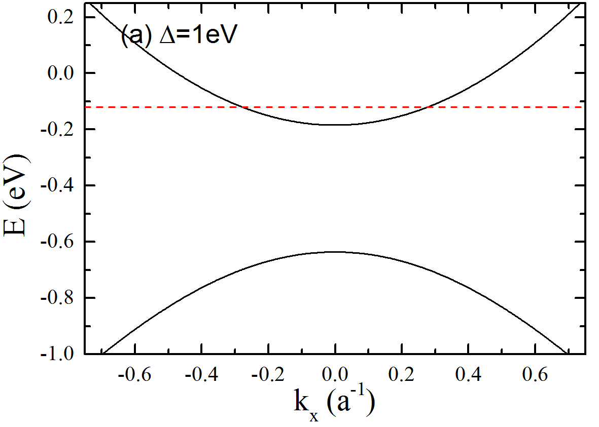
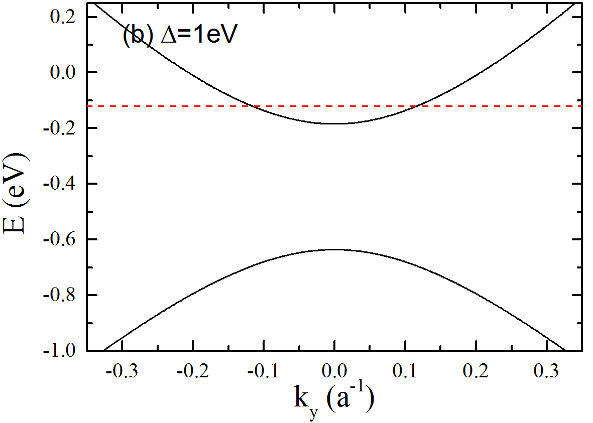
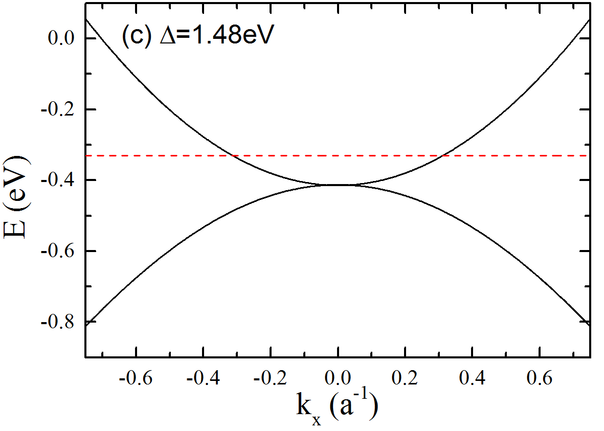
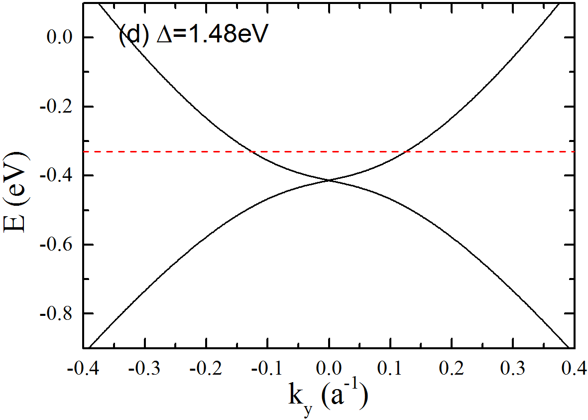
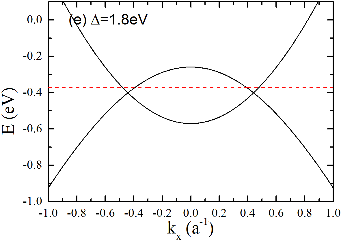
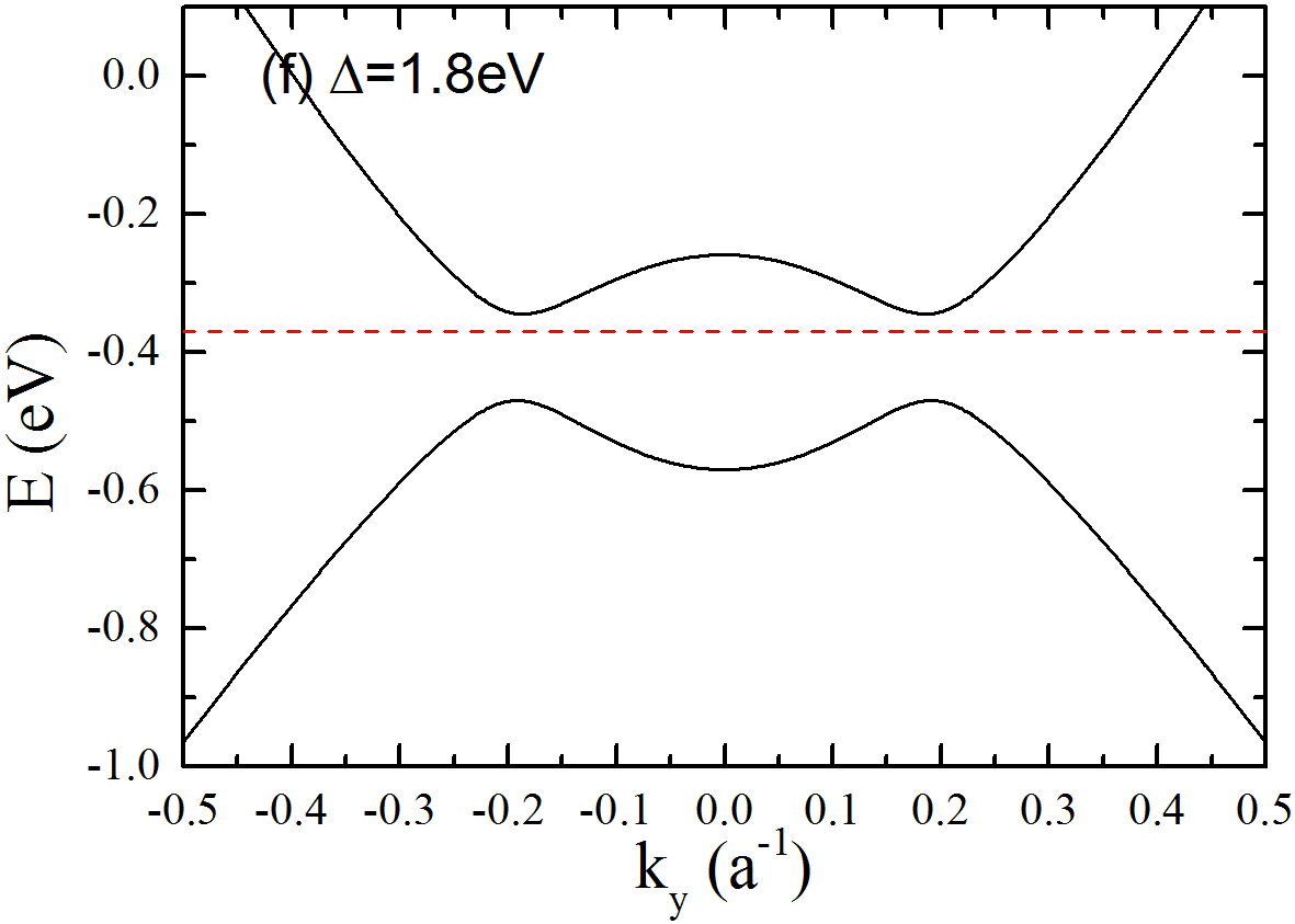
Figure 8: Low energy band structure of bilayer BP in the presence of a perpendicular electric field, for different biased potential energy between top and bottom layers. The red dashed line in each panel indicates the position of the chemical potential in the calculation of the plasmon modes.

Our results show that the velocity of the plasmon mode increases with the biased voltage, as it can be seen from the evolution of the excitation spectrum with the applied $\Delta$ in Fig. 9. This suggest the possibility to tune the plasmonic properties of this material with a perpendicular electric field. Interestingly, when the applied electric field exceeds the critical field and enters in the topological phase, the plasmons are more coherent, as it can be inferred by looking at the strength of the modes in the density plots of Fig. 9 (notice the different scales in the density bar of each panel). Furthermore, the plasmon dispersion is ungapped along $q_{x}$ direction, whereas the presence of a gap in the electronic band structure in the $\Gamma-$Y direction leads to a gapped collective mode along $q_{y}$, as it can be seen by looking Fig. 9(f) in the low energy and small wave-vector region. We notice again that, due to the finite size nature of our simulations, our results cannot reach the $q\rightarrow 0$ limit, for which we would need to consider an infinite sample. However, the existence of a gap in the plasmon spectrum $q_{y}$ direction is already clear in the present calculation for $\Delta=1.8$ eV. Notice that the peculiar band structure in the topological phase, with Dirac like band crossings in one direction and gap in the other direction, leads to a rich excitation spectrum with a numerous peaks corresponding to the plasmon collective excitations and to the enhanced optical transitions due to appearance of Van Hove singularities in the spectrum.

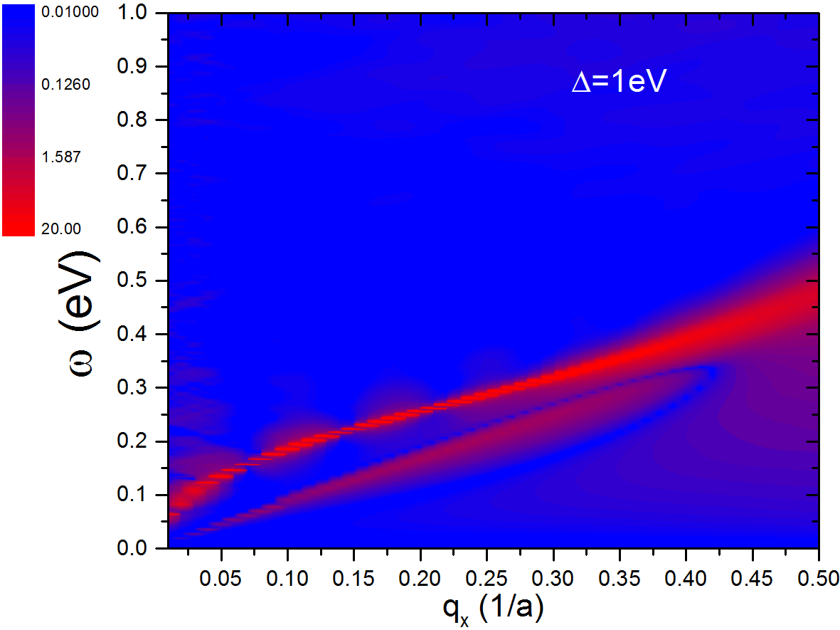
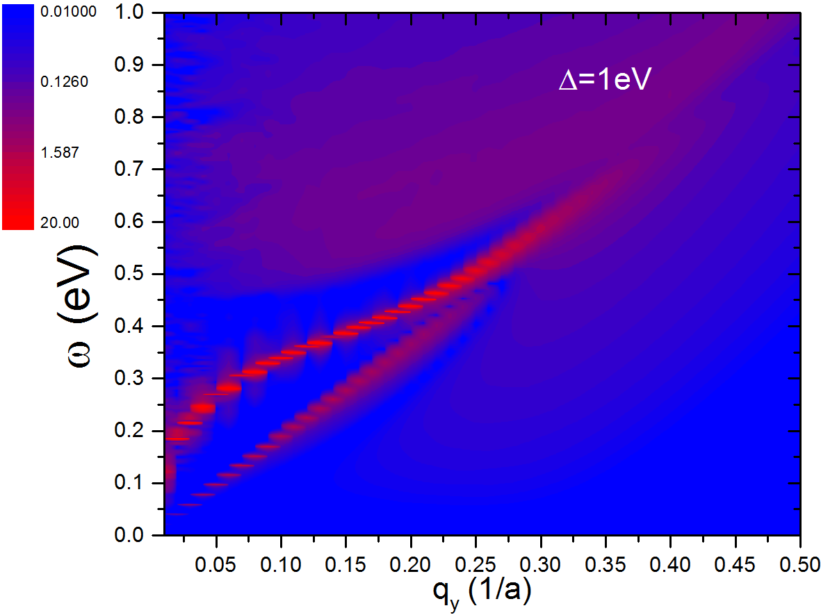
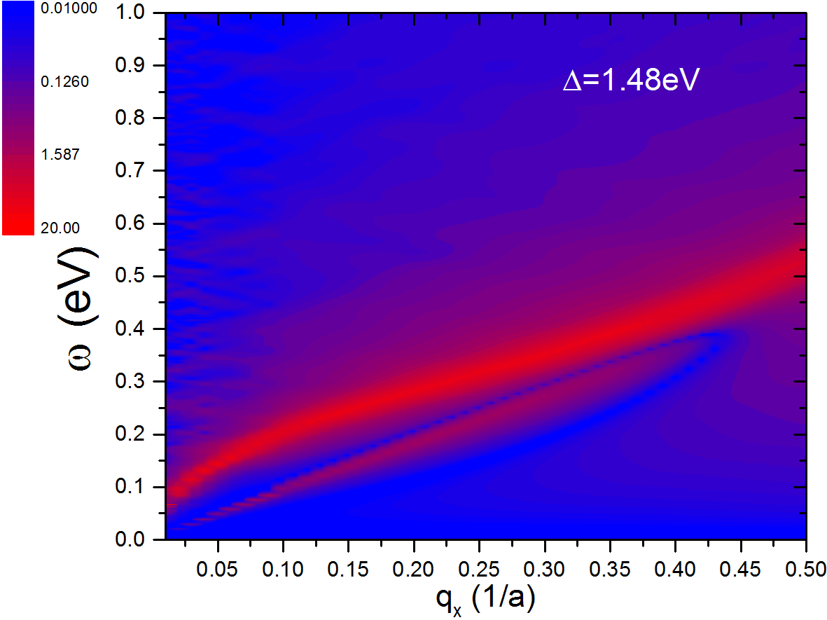
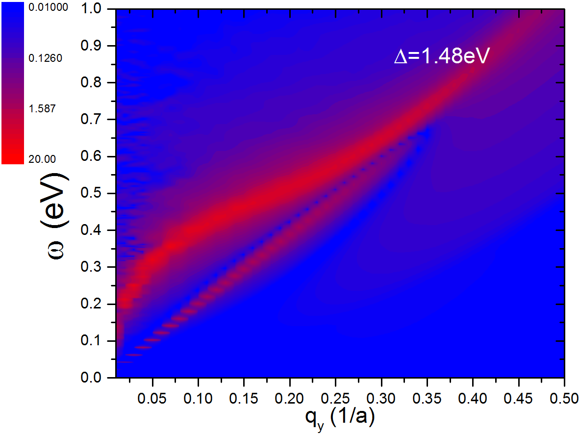
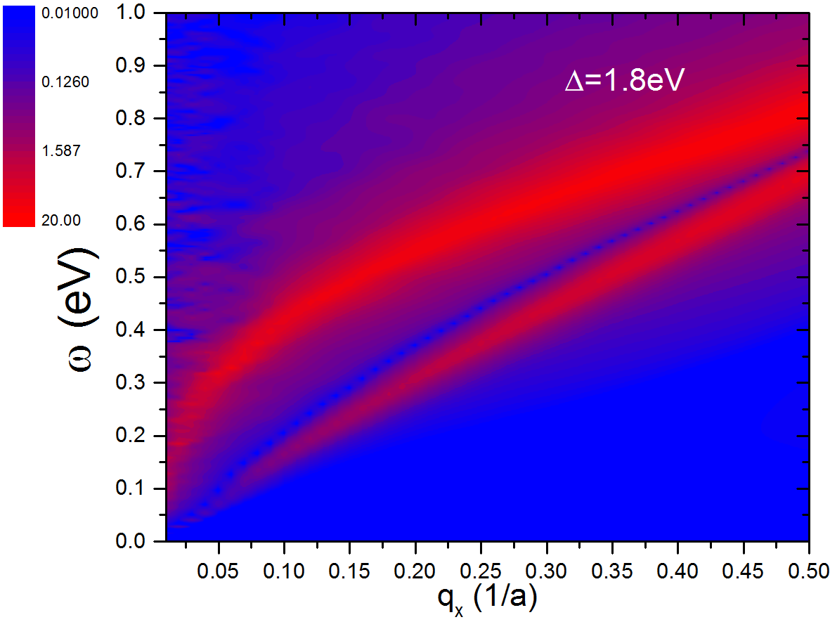
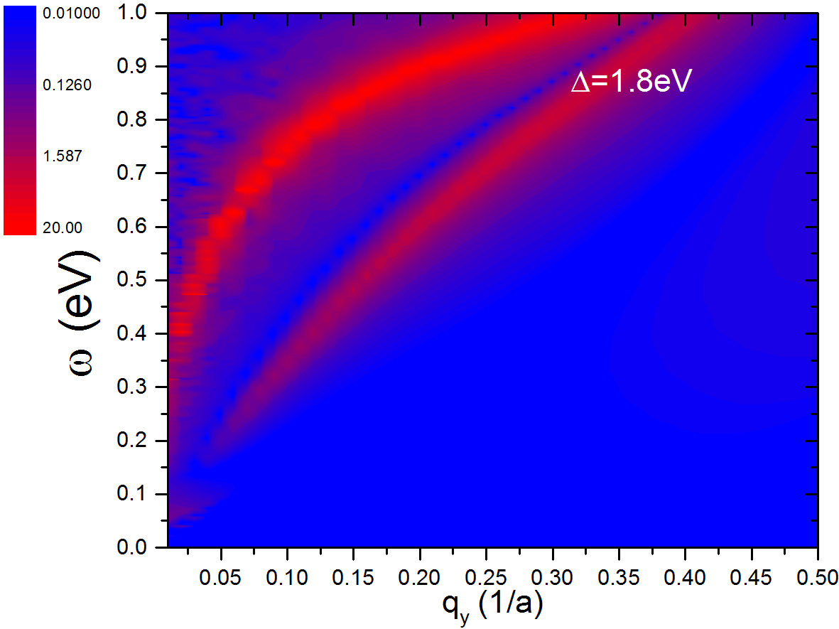
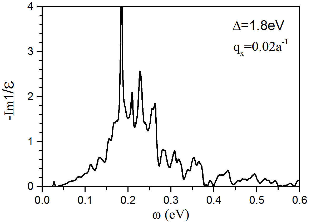
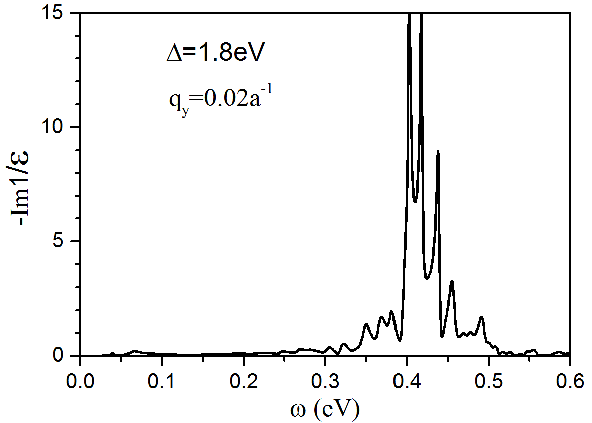
Figure 9: Energy loss functions of biased bilayer BP along zigzag (left) and armchair (right) directions. The strength of the biased potential is given in each panel.

V Conclusions

In conclusion, we have studied the effect of disorder in the excitation spectrum of single-layer and bilayer BP. The band structure has been calculated with an accurate tight-binding model which is valid within $\sim 0.3$ eV beyond the gap. The dynamical polarization function has been calculated with the Kubo formula, and from this, the energy loss function has been obtained within the RPA. We have found that disorder leads to a redshift of the plasmon resonance. This effect has been discussed from a perturbative point of view, within the framework of the disordered averaged response function.Mermin (1970)

The different kinds of disordered that have been analyzed show that, for the same concentration of impurities, LRPD leads to stronger damping rates as compared to local point defects. Such effect is understood from the intrinsic long wavelength nature of the plasmon oscillations, induced by long range Coulomb interaction. Therefore resonant scatterers as point vacancies, which modify the electronic properties at very short length scales, are less effective inducing losses of the plasmon modes than LRPD.

The spectrum of bilayer BP presents two plasmon modes. One mode in which the carrier density in the two planes oscillates in-phase, with a dispersion $\omega_{+}(q)\sim\sqrt{q}$, which is the counterpart of the standard plasmon in single-layer BP, and one mode in which the carriers in the two layers oscillate out-of-phase, with a liner dispersion relation at low energies, $\omega_{-}(q)\sim q$. The coherence of the $\omega_{-}$ mode is more dramatically affected by disorder.

Finally, we have studied the effect of a perpendicular electric field in the excitation spectrum of bilayer BP. We have shown that the dispersion of the collective modes can be tuned by the application of such biased field. Furthermore, we have shown that, beyond some critical field, the bilayer BP enters in a topological phase with Dirac like crossing of bands in one direction and gapped in the other direction. As a consequence, the excitation spectrum is highly rich in this limit, with highly coherent plasmon modes which are gapped in the $q_{y}$ direction of the spectrum. In summary, our results show a highly anisotropic excitation spectrum of single layer and bilayer BP, features that could be of high interest for future optoelectronic applications.

VI Acknowledgments

The support by the Stichting Fundamenteel Onderzoek der Materie (FOM) and the Netherlands National Computing Facilities foundation (NCF) are acknowledged. S.Y. and M.I.K. thank financial support from the European Research Council Advanced Grant program (contract 338957). The research has also received funding from the European Union Seventh Framework Programme under Grant Agreement No. 604391 Graphene Flagship. R.R. acknowledges support from the European Research Council Advanced Grant (contract 290846).

References

- Li et al. (2014) L. Li, Y. Yu, G. J. Ye, Q. Ge, X. Ou, H. Wu, D. Feng, X. H. Chen, and Y. Zhang, Nat. Nanotech. 9, 372 (2014).
- Liu et al. (2014a) H. Liu, A. T. Neal, Z. Zhu, Z. Luo, X. Xu, D. Tománek, and P. D. Ye, ACS Nano 8, 4033 (2014a).
- Xia et al. (2014) F. Xia, H. Wang, and Y. Jia, Nat. Commun. 5, 4458 (2014).
- Koenig et al. (2014) S. P. Koenig, R. A. Doganov, H. Schmidt, A. H. Castro Neto, and B. Özyilmaz, Appl. Phys. Lett. 104, 103106 (2014).
- Castellanos-Gomez et al. (2014) A. Castellanos-Gomez, L. Vicarelli, E. Prada, J. O. Island, K. L. Narasimha-Acharya, S. I. Blanter, D. J. Groenendijk, M. Buscema, G. A. Steele, J. V. Alvarez, et al., 2D Materials 1, 025001 (2014).
- Li et al. (2014) L. Li, G. J. Ye, V. Tran, R. Fei, G. Chen, H. Wang, J. Wang, K. Watanabe, T. Taniguchi, L. Yang, et al., ArXiv e-prints (2014), eprint 1411.6572.
- Morita (1986) A. Morita, Applied Physics A 39, 227 (1986).
- Ling et al. (2015) X. Ling, H. Wang, S. Huang, F. Xia, and M. S. Dresselhaus, Proceedings of the National Academy of Sciences 112, 4523 (2015).
- Qiao et al. (2014) J. Qiao, X. Kong, Z.-X. Hu, F. Yang, and W. Ji, Nat. Commun. 5, 4475 (2014).
- Rudenko and Katsnelson (2014) A. N. Rudenko and M. I. Katsnelson, Phys. Rev. B 89, 201408 (2014).
- Guan et al. (2014) J. Guan, Z. Zhu, and D. Tománek, Phys. Rev. Lett. 113, 046804 (2014).
- Peng et al. (2014) X. Peng, Q. Wei, and A. Copple, Phys. Rev. B 90, 085402 (2014).
- Tran et al. (2014) V. Tran, R. Soklaski, Y. Liang, and L. Yang, Phys. Rev. B 89, 235319 (2014).
- Çakır et al. (2014) D. Çakır, H. Sahin, and F. M. Peeters, ArXiv e-prints (2014), eprint 1411.1344.
- Low et al. (2014a) T. Low, A. S. Rodin, A. Carvalho, Y. Jiang, H. Wang, F. Xia, and A. H. Castro Neto, Phys. Rev. B 90, 075434 (2014a).
- Low et al. (2014b) T. Low, M. Engel, M. Steiner, and P. Avouris, Phys. Rev. B 90, 081408 (2014b).
- Li and Appelbaum (2014) P. Li and I. Appelbaum, Phys. Rev. B 90, 115439 (2014).
- Yuan et al. (2015) S. Yuan, A. N. Rudenko, and M. I. Katsnelson, Phys. Rev. B 91, 115436 (2015).
- Rodin et al. (2014) A. S. Rodin, A. Carvalho, and A. H. Castro Neto, Phys. Rev. Lett. 112, 176801 (2014).
- Elahi et al. (2015) M. Elahi, K. Khaliji, S. M. Tabatabaei, M. Pourfath, and R. Asgari, Phys. Rev. B 91, 115412 (2015).
- Roldán et al. (2015) R. Roldán, A. Castellanos-Gomez, E. Cappelluti, and F. Guinea, J. Phys.: Condens. Matter 27, 313201 (2015).
- Low et al. (2014c) T. Low, R. Roldán, H. Wang, F. Xia, P. Avouris, L. M. Moreno, and F. Guinea, Phys. Rev. Lett. 113, 106802 (2014c).
- Rodin and Castro Neto (2015) A. S. Rodin and A. H. Castro Neto, Phys. Rev. B 91, 075422 (2015).
- Jiang et al. (2015) Y. Jiang, R. Roldán, F. Guinea, and T. Low, arXiv preprint arXiv:1505.00175 (2015).
- Favron et al. (2014) A. Favron, E. Gaufrès, F. Fossard, P. L. Lévesque, A. Phaneuf-L’Heureux, N. Y-W. Tang, A. Loiseau, R. Leonelli, S. Francoeur, and R. Martel, ArXiv e-prints (2014), eprint 1408.0345.
- Wood et al. (2014) J. D. Wood, S. A. Wells, D. Jariwala, K.-S. Chen, E. Cho, V. K. Sangwan, X. Liu, L. J. Lauhon, T. J. Marks, and M. C. Hersam, Nano Letters 14, 6964 (2014).
- Island et al. (2015) J. O. Island, G. A. Steele, H. S. J. van der Zant, and A. Castellanos-Gomez, 2D Materials 2, 011002 (2015).
- Yuan et al. (2010a) S. Yuan, H. De Raedt, and M. I. Katsnelson, Phys. Rev. B 82, 115448 (2010a).
- Yuan et al. (2011a) S. Yuan, R. Roldán, and M. I. Katsnelson, Phys. Rev. B 84, 035439 (2011a).
- Yuan et al. (2012) S. Yuan, T. O. Wehling, A. I. Lichtenstein, and M. I. Katsnelson, Phys. Rev. Lett. 109, 156601 (2012).
- Neto et al. (2009) A. H. C. Neto, F. Guinea, N. M. R. Peres, K. S. Novoselov, and A. K. Geim, Rev. Mod. Phys 81, 109 (2009).
- Das Sarma et al. (2011) S. Das Sarma, S. Adam, E. H. Hwang, and E. Rossi, Rev. Mod. Phys. 83, 407 (2011).
- Katsnelson (2012) M. I. Katsnelson, Graphene: Carbon in Two Dimensions (Cambridge University Press, 2012).
- Yuan et al. (2010b) S. Yuan, H. De Raedt, and M. I. Katsnelson, Phys. Rev. B 82, 235409 (2010b).
- Qiu et al. (2013) H. Qiu, T. Xu, Z. Wang, W. Ren, H. Nan, Z. Ni, Q. Chen, S. Yuan, F. Miao, F. Song, et al., Nat. Commun. 4, 2642 (2013).
- Yuan et al. (2014) S. Yuan, R. Roldán, M. I. Katsnelson, and F. Guinea, Phys. Rev. B 90, 041402 (2014).
- Liu et al. (2014b) Y. Liu, F. Xu, Z. Zhang, E. S. Penev, and B. I. Yakobson, Nano Letters 14, 6782 (2014b).
- Hu and Yang (2014) W. Hu and J. Yang, ArXiv e-prints (2014), eprint 1411.6986.
- Kulish et al. (2015) V. V. Kulish, O. I. Malyi, C. Persson, and P. Wu, Phys. Chem. Chem. Phys. 17, 992 (2015).
- Zhang et al. (2014) R. Zhang, B. Li, and J. Yang, ArXiv e-prints (2014), eprint 1409.7190.
- Ziletti et al. (2015) A. Ziletti, A. Carvalho, D. K. Campbell, D. F. Coker, and A. H. Castro Neto, Phys. Rev. Lett. 114, 046801 (2015).
- Lewenkopf et al. (2008) C. H. Lewenkopf, E. R. Mucciolo, and A. H. Castro Neto, Phys. Rev. B 77, 081410 (2008).
- Yuan et al. (2011b) S. Yuan, R. Roldán, H. De Raedt, and M. I. Katsnelson, Phys. Rev. B 84, 195418 (2011b).
- Hwang et al. (2007) E. H. Hwang, S. Adam, and S. Das Sarma, Phys. Rev. Lett. 98, 186806 (2007).
- Zhang et al. (2009) Y. Zhang, V. W. Brar, C. Girit, A. Zettl, and M. F. Crommie, Nature Phys. 5, 722 (2009).
- Rudenko et al. (2011) A. N. Rudenko, F. J. Keil, M. I. Katsnelson, and A. I. Lichtenstein, Phys. Rev. B 84, 085438 (2011).
- Principi et al. (2013) A. Principi, G. Vignale, M. Carrega, and M. Polini, Phys. Rev. B 88, 121405 (2013).
- Gibertini et al. (2010) M. Gibertini, A. Tomadin, M. Polini, A. Fasolino, and M. I. Katsnelson, Phys. Rev. B 81, 125437 (2010).
- Gibertini et al. (2012) M. Gibertini, A. Tomadin, F. Guinea, M. I. Katsnelson, and M. Polini, Phys. Rev. B 85, 201405 (2012).
- Kubo (1957) R. Kubo, J. Phys. Soc. Jpn. 12, 570 (1957).
- Hams and De Raedt (2000) A. Hams and H. De Raedt, Phys. Rev. E 62, 4365 (2000).
- Politano and Chiarello (2014) A. Politano and G. Chiarello, Nanoscale 6, 10927 (2014).
- Mermin (1970) N. D. Mermin, Phys. Rev. B 1, 2362 (1970).
- Agarwal and Vignale (2015) A. Agarwal and G. Vignale, Phys. Rev. B 91, 245407 (2015).
- Giuliani and Vignale (2005) G. F. Giuliani and G. Vignale, Quatum Theory of the Electron Liquid (CUP, Cambridge, 2005).
- Das Sarma and Hwang (1998) S. Das Sarma and E. H. Hwang, Phys. Rev. Lett. 81, 4216 (1998).
- Gamayun (2011) O. V. Gamayun, Phys. Rev. B 84, 085112 (2011).
- Roldán and Brey (2013) R. Roldán and L. Brey, Phys. Rev. B 88, 115420 (2013).
- Liu et al. (2015) Q. Liu, X. Zhang, L. B. Abdalla, A. Fazzio, and A. Zunger, Nano Letters 15, 1222 (2015).
- Dolui and Quek (2015) K. Dolui and S. Y. Quek, ArXiv e-prints (2015), eprint 1503.03647.
- Pereira and Katsnelson (2015) J. M. Pereira, Jr. and M. I. Katsnelson, ArXiv e-prints (2015), eprint 1504.02452.