The long-tail distribution function of mutations in bacteria

Abstract

Levy flights in the space of mutations model time evolution of bacterial DNA. Parameters in the model are adjusted in order to fit observations coming from the Long Time Evolution Experiment with E. Coli.

The Long Time Evolution Experiment. I recall the extremely interesting experiment with E. Coli, conducted by Prof. R. Lenski and his group ref1 ; ref2 , and running already for more than 27 years. Among the reported results, I use the following ref3 :

1. In a culture of bacteria, after 20,000 generations, around $3\times 10^{8}$ single point mutations in the DNA are registered. These are local modifications of the DNA chain. I notice that the number of bacteria undergoing continuous evolution is around $5\times 10^{6}$.

2. They measure also the frequency of mutations involving rearrangements in segments of the DNA. In particular, mutations in which the repair mechanisms are damaged and the mutation rate increases 100 times. This mutator phenotype becomes dominant in two of twelve cultures (probability 1/6) after 2500 - 3000 generations, in a third culture (cumulative probability 1/4) after 8,500 generations, and in a fourth culture (cumulative probability 1/3) after 15,000 generations.

The purpose of my paper is to present a model for mutations in bacteria and to adjust the model parameters in order to qualitatively fit these data.

The accumulative character of mutations.

In my model, the time evolution of cells defines trajectories, as schematically represented in Fig. 1, where two of these trajectories are drawn in red.

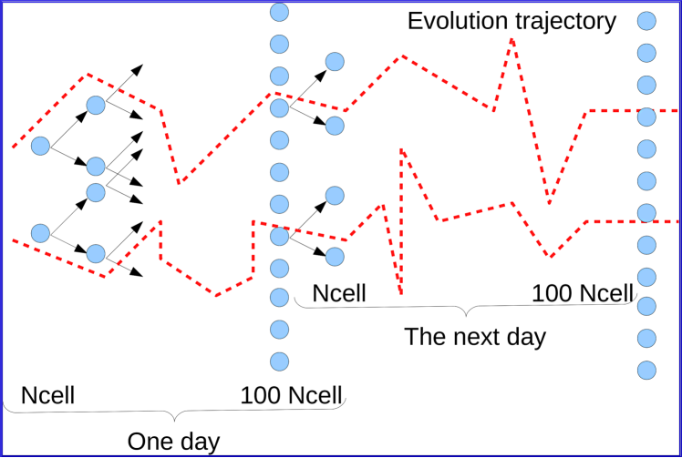
Figure 1: Schematic representation of the evolution of bacteria in the Long Time Evolution Experiment. Every day, the cells experience a clonal expansion in which the initial number $N_{cell}\approx 5\times 10^{6}$ is raised 100 times. However, only $N_{cell}$ bacteria pass to the next day. The evolution trajectories of two cells are marked by red dashed lines.

The idea about trajectories in the evolution of cells means that there are Markov chains ref4 of mutations, where the change in the DNA of a cell at step $i+1$, $x_{i+1}$, comes from the change in the previous step plus an additional modification:

$$x_{i+1}=x_{i}+\delta$$ (1)

Horizontal DNA transfer is not considered.

Measuring changes in the DNA A single strand of E. Coli DNA contains around $4.6\times 10^{6}$ bases of a four letter alphabet: A, G, C, and T. ref5 In order to measure changes in the DNA, one may use a variable similar to that one of paper ref6 .

First, define an auxiliary variable at site $\alpha$ in the molecule: $u_{\alpha}(G)=3/8$, $u_{\alpha}(A)=1/8$, $u_{\alpha}(T)=-1/8$, and $u_{\alpha}(C)=-3/8$. Then, define a walk along the DNA:

$$y(\beta)=\sum_{\alpha=1}^{\beta}u_{\alpha}.$$ (2)

As a function of $\beta$, the variable $y$ draws a profile of the DNA molecule, and modifications can be measured as: $X(\beta)=y(\beta)-y_{0}(\beta)$. where $y$ correspond to the mutated DNA, and $y_{0}$ – to the initial configuration. Of course, there are so many $X(\beta)$, five millions, that they are not of practical use. The strategy could be to use variables measuring global changes or distances to the original function:

$$X=\sum_{\alpha=1}^{L}(u^{\prime}_{\alpha}-u_{\alpha}),$$ (3)

$$X^{(1)}=\sum_{\alpha=1}^{L}\alpha(u^{\prime}_{\alpha}-u_{\alpha}),$$ (4)

$X^{(2)}$ (the second moment), etc. $L$ is the length of the molecule. The Shannon informational entropy ref7 could also be of use.

In what follows, I shall assume that mutations are well characterized by a few global variables.

Levy model of mutations The $\delta$ term in Eq. (1) represents mutations at step $i+1$. It may come from a partially repaired damage in the DNA that is fixed after replication, or from a prune error in the replication process. It should be stressed that both the repair mechanisms and the replication process guarantee very high fidelities. The error introduced by the latter, for example, is around one mistaken base per $10^{9}$ bases in the human DNA strand ref8 .

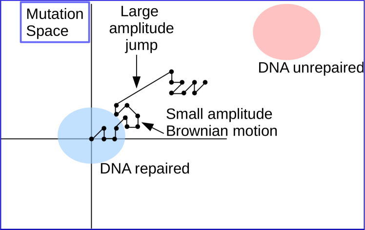
Figure 2: Schematic representation of a single cell mutation trajectory. The starting point is $X=0$. In the mutation space, I distinguished regions in which the DNA repair mechanism is active or damaged.

Let me stress once again that $\delta$ is not the damage caused by endogenous or external factors, but the resulting modification after the action of the repair mechanisms. It is known, for example, that ionizing radiation may cause double strand breaks in the DNA ref9 . These damages are very difficult to repair ref8 . The repair mechanism itself may introduce large changes in the resulting DNA composition after a double strand break event.

My proposal for $\delta$ is the following: $\delta=\delta_{B}+\delta_{LJ}$. The $\delta_{B}$ component corresponds to a Brownian motion with maximal amplitude $D_{B}$. Notice that $D_{B}=1$ would mean roughly a change of basis in each replication step because $u_{\alpha}(G)-u_{\alpha}(C)=3/4$. This Brownian motion introduces local modifications in the DNA. After $N_{step}$ replication steps, the characteristic dispersion of a trajectory due to this Brownian motion (something like the radius of the colored region near the origin in Fig. 2) is $D_{B}\sqrt{N_{step}}$. ref10

The large-jump component of $\delta$, $\delta_{LJ}$, on the other hand, is modeled with the help of rare events with total probability $p<<1$, and a probability density proportional to $1/\delta_{LJ}^{2}$, where the amplitude ranges from $D_{B}$ to infinity (in practice, I will introduce a cutoff, $D_{max}$). The combination of the Brownian motion and the large amplitude jumps leads to Levy flights ref11 in the mutation space, schematically represented in Fig. 2.

Let me notice that the distribution function associated to Levy flights is a fat- or long-tail one. This fact could be related to the long range correlations observed in the walks along the DNA ref6 .

The long-tail distribution function of mutations. Four parameters enter my oversimplified Levy model of mutations: $N_{cell}$, $N_{step}$, $D_{B}$ and $p$. As mentioned above, $N_{cell}=4.6\times 10^{6}$. On the other hand, $N_{step}$ is the number of replication steps along a trajectory.

$D_{B}$ is the amplitude of the Brownian motion. It shall be determined from the observed number of single point mutations (SPM) after 20,000 generations. The number of SPMs per bacteria is $3\times 10^{8}/(4.6\times 10^{6})\approx 65$. The characteristic dispersion of the trajectory, on his side, is the Brownian radius, $\sqrt{N_{step}}~{}D_{B}\approx 140~{}D_{B}$. In order to estimate que equivalent number of SPM, I divide the latter by the mean deviation involved in a SPM, that is 5/12. Notice that $u(G)-u(A)=1/4$, $u(G)-u(T)=1/2$, etc. Thus, $65=140~{}D_{B}/(5/12)$, and $D_{B}\approx 0.19$.

Finally, the parameter $p$ is fixed to $1.3\times 10^{-5}$ Below, I shall come back to the way of determining it.

In the simulations, all of the $N_{cell}$ trajectories start at $X=0$. In any replication step, mutations are given by Eq. (1), where $\delta$ contains both the Brownian and the large-amplitude components.

The probability distribution function for mutations in a cell, $P(X)$, is the probability that a cell arrives at the end point with an amplitude $X$. For convenience, I compute not $P(X)$, but the cumulative probability distribution, $P(|X|>Z)$, which is shown in Fig. 3 for $N_{step}=3000$.

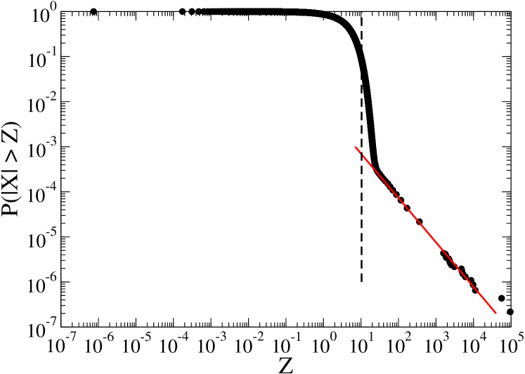
Figure 3: The average cumulative probability of mutations, $P(|X|>Z)$, for a single bacterium after 3000 generations. Points come from the numerical simulations, whereas the red solid line is a $1/Z$ fit to the tail. The Brownian radius, $D_{B}\sqrt{N_{step}}$, is marked by a dashed line.

The Brownian radius, $\sqrt{N_{step}}~{}D_{B}\sim 10.4$, concentrating most of the points, is apparent in the figure. In addition, the tail can be fitted to a $1/Z$ dependence. The coefficient is roughly $N_{step}D_{B}~{}p$.

The data on the mutator phenotype is to be used in order to fix the slope in the tail. I assume that the repair mechanisms are related to a coding region in the DNA of length $l$. The mechanisms are damaged when this region suffers modifications greater than a given $X_{u}$. The cumulative probability can be estimated as $N_{cell}~{}P(|X|>X_{u})$. Using the functional dependence in the tail, I get:

$$Cum.~{}Prob.\approx N_{cell}\frac{N_{step}D_{B}~{}p}{X_{u}}\frac{l}{L}=aN_{cell}N_{step}.$$ (5)

So far, I do not have precise values for $l$ and $X_{u}$. Reasonable numbers are $l/L\approx 10^{-2}$, $X_{u}/L\approx 10^{-3}$. From the observed probabilities, I get $a\approx 5.4\times 10^{-12}$, as shown in Fig. 4, from which it follows that $p=1.3\times 10^{-5}$.

The asymptotic formula for events in the tail of the distribution, Eq. (5), is valid no matter how precise are $l$ and $X_{unrep}$.

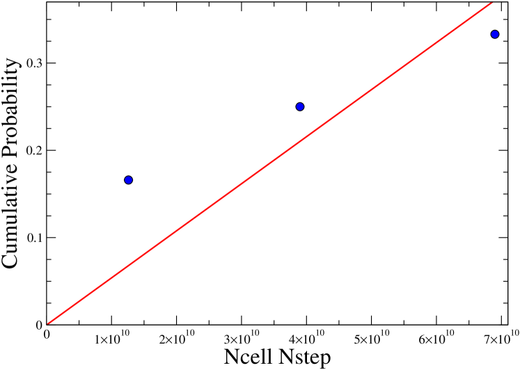
Figure 4: Cumulative probability of the mutator phenotype in the Long Time Evolution Experiment. The line is a fit according to Eq. (5).

Mutations and natural selection. Let me stress that in Fig. 4 probabilities are measured in a set of 12 cultures. Thus, one expects errors of the order of $1/\sqrt{12}\approx 0.3$. In addition, Lenski and his group report not the occurrence of the mutation, but the moment at which the phenotype becomes dominant in a population. In this process, natural selection plays a major role.

In both the DNA-repaired and DNA-unrepaired regions of the mutation space, there exist points with evolutive advantage. These points act as attractors in the mutation space.

Natural selection may be included in my model by introducing a relative fitness parameter, $w$. ref12 $w_{r}=1$ and $w_{u}$ apply to regions of radius three around the centers of the DNA-repaired and DNA-unrepaired areas. Out of these regions, $w_{o}=0.7$. I introduce a clonal expansion phase in which the number of cells increases 100 times, as in the Lenski experiment, but only $N_{cell}$ bacteria pass to the next step. The bacteria are selected according to the conditional probability $w/(w_{o}+w_{r}+w_{u})$. Results are to be published elsewhere ref13 .

Levy model of cancer. With appropriate parameters, my Levy model can also be applied to mutations in stem cells and, in particular, to the analysis of lifetime cancer risk in different tissues ref14 with the help of a formula like Eq. (5). Results are to be published elsewhere. ref15

I would like to stress only the intriguing fact that in cases, like the ovarian germinal cell cancer, where physical barriers act as protection, and the action of the immune system is partially depressed, the slope $a$ takes values similar to the number obtained for bacteria.

Acknowledgments. The author acknowledges support from the National Program of Basic Sciences in Cuba, and from the Office of External Activities of the International Centre for Theoretical Physics (ICTP).

References

- (1) R.E. Lenski, Summary data from the long-term evolution experiment, http://myxo.css.msu.edu/ecoli/summdata.html
- (2) A brief description can also be found in A. Gonzalez, Rev. Cub. Fis. 31, 71 (2014).
- (3) R.E. Lenski, Phenotypic and genomic evolution during a 20000 generation experiment with the bacterium E. Coli, in J. Janick, Ed., Plant Breeding Reviews, Vol. 24, Part 2, page 225, 2004.
- (4) V.S. Koroliuk, N.I. Portenko, A.V. Skorojod, and A.F. Turbin, Handbook on probability theory and mathematical statistics, Nauka, Moscow 1978.
- (5) F.R. Blattner, G. Plunkett, C.A. Bloch, et. al., The complete genome sequence of Escherichia Coli K-12, Science 277, 1453–62 (1977).
- (6) C.-K. Peng, S.V. Buldyrev, A.L. Goldberger, et. al., Physica A 191, 25 (1992).
- (7) T. D. Schneider. Information and entropy of patterns in genetic switches. In G. J. Erickson and C. R. Smith, Eds., Maximum-Entropy and Bayesian Methods in Science and Engineering, volume 2, pages 147–154, Dordrecht, Kluwer Academic, 1988.
- (8) Molecular Biology of the Cell, B. Alberts, A. Johnson, J. Lewis, M. Raff, K. Roberts, and P. Walter, New York: Garland Science, 2002.
- (9) Leon Mullenders, Mike Atkinson, Herwig Paretzke, Laure Sabatier and Simon Bouffler, Nature Reviews Cancer 9, 596 - 604 (2009).
- (10) A. Einstein, Investigations on the theory of the Brownian movement, Dover, 1956.
- (11) Levy flights and related phenomena in Physics, Eds. M.F. Shlesinger, G. Zaslavsky, and U. Frish, Lecture Notes in Physics, Vol. 450, Springer, Berlin 1995.
- (12) H. Allen Orr, Nature Reviews Genetics 10, 531 (2009).
- (13) Leo Cruz and A. Gonzalez, to be submitted.
- (14) C. Tomasetti and B. Vogelstein, Science 347, 78 - 81 (2015); Supplementary materials: www.sciencemag.org/content/347/6217/78/suppl/
- (15) A. Gonzalez, Levy model of cancer, submitted.