Determining solubility for finitely generated groups of PL homeomorphisms

Abstract.

The set of finitely generated subgroups of the group $PL_{+}(I)$ of orientation-preserving piecewise-linear homeomorphisms of the unit interval includes many important groups, most notably R. Thompson’s group $F$. In this paper we show that every finitely generated subgroup $G<PL_{+}(I)$ is either soluble, or contains an embedded copy of Brin’s group $B$, a finitely generated, non-soluble group, which verifies a conjecture of the first author from 2009. In the case that $G$ is soluble, we show that the derived length of $G$ is bounded above by the number of breakpoints of any finite set of generators. We specify a set of ‘computable’ subgroups of $PL_{+}(I)$ (which includes R. Thompson’s group $F$) and we give an algorithm which determines in finite time whether or not any given finite subset $X$ of such a computable group generates a soluble group. When the group is soluble, the algorithm also determines the derived length of $\langle X\rangle$. Finally, we give a solution of the membership problem for a family of finitely generated soluble subgroups of any computable subgroup of $PL_{+}(I)$.

1. Introduction

In [4, 2, 1, 3] a theory is built connecting the solubility class of a subgroup $G$ of the group $PL_{+}(I)$ of piecewise-linear orientation-preserving homeomorphisms of $I=[0,1]$ (with finitely many breaks in slope) with data on how the supports of the elements of $G$ overlap with each other, and how these supports relate to the support of the whole action of $G$ on $I$. One result in that theory is that there is a non-soluble group $W$ which is not finitely generated, and which contains an embedded copy of every soluble subgroup of $PL_{+}(I)$, such that any non-soluble subgroup of $PL_{+}(I)$ contains an embedded copy of $W$ (Corollary 1.2 and Theorem 1.1, respectively, of [3]). However, in the finitely generated case, it has been believed that one could considerably strengthen that result. Indeed, it is conjectured in [3] that any finitely generated non-soluble subgroup of $PL_{+}(I)$ contains an embedded copy of Brin’s group $B$, a two-generated non-soluble group introduced by Brin in Section 5 of [5] as $G_{1}$. In this paper we verify this conjecture.

To be more specific, we say that $G$ admits a transition chain if there are two elements $g,h\in G$ with components of support $(a,b),(c,d)$, respectively, such that $a<c<b<d$. If $G$ does not admit such a chain, then we say that $G$ is chainless. In a similar fashion, the group $G$ admits a one-sided overlap if there are two elements $g,h\in G$ with components of support $(a,b),(a,c)$ or $(a,b),(c,b)$, respectively, such that $a<c<b$. Finally, $G$ admits a tower of infinite height if there is an infinite sequence $\{g_{i}\}_{i\in\mathbb{N}}$ of elements of $G$ with components of support $A_{i}$, respectively, such that $A_{i+1}\subsetneq A_{i}$ for all $i$. We illustrate these three properties in the special case of elements with a single component of support in Figure 1.

In [2, Theorem 1.1 and Lemma 1.4] (restated with further details in Theorem 2.2 and Lemma 2.3 of Section 2.2 below) the first author shows that a soluble subgroup of $PL_{+}(I)$ must be chainless and does not admit a tower of infinite height. In our main theorem (Theorem 3.2) in Section 3 below, we show that in the finitely generated case the converse of each of these also holds. In Lemma 3.1 we show that for a subgroup $G\leq PL_{+}(I)$ generated by a finite set $X\subset PL_{+}(I)$, the number of $G$-orbits of the set of breakpoints of elements of $G$ is bounded above by the cardinality of the set of breakpoints of the elements of $X$ (a point $x\in(0,1)$ is a breakpoint of $g\in PL_{+}(I)$ if $g$ changes slope at $x$); this is applied in Theorem 3.2 to obtain a bound on the derived length in the soluble case.

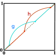
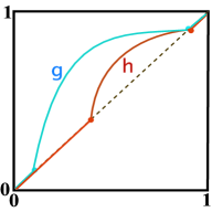
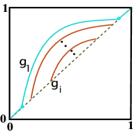
Figure 1. Transition chain, one-sided overlap, and tower of infinite height

Theorem 3.2. Let $G<PL_{+}(I)$ be generated by a finite set $X$. The following are equivalent.

1. $G$ is not soluble.

2. $G$ admits a transition chain.

3. $G$ admits a one-sided overlap.

4. $G$ admits a tower of infinite height.

Moreover, if $G$ is soluble, the derived length of $G$ is less than or equal to the cardinality of the set $\mathscr{B}_{X}$ of breakpoints of elements of $X$.

Our first application of Theorem 3.2 is a verification of the conjecture discussed in the first paragraph of this introduction. Note that since a soluble group cannot contain a non-soluble subgroup, a subgroup $G\leq PL_{+}(I)$ containing a copy of $B$ is also non-soluble. Theorem 1.4 of [3] (restated in Theorem 2.7 in Section 2.4) states that if $G$ admits a transition chain, then it admits an embedded copy of Brin’s group $B$, and so we obtain the following corollary resolving the conjecture.

Corollary 1.1.

Let $G$ be a finitely generated subgroup of $PL_{+}(I)$. Then $G$ is non-soluble if and only if Brin’s group $B$ embeds in $G$.

Thus $B$ not only contains every soluble subgroup of $PL_{+}(I)$, but $B$ is also contained in every finitely generated non-soluble subgroup of $PL_{+}(I)$.

In Section 4 we apply Theorem 3.2 to develop a solution to the soluble subgroup recognition problem (SSRP). Given a group $G$ with a finite generating set $Y$, the SSRP asks whether there is an algorithm that, upon input of a finite set $X$ of words over $Y^{\pm 1}$, can determine whether or not the subgroup $\langle X\rangle$ of $G$ generated by $X$ is a soluble group. For a subgroup $G<PL_{+}(I)$, we allow the the finite list $X$ of elements input into our procedure to have formats other than a list of words over a finite generating set of $G$; for example, if $G$ is R. Thompson’s group $F$, in which all breakpoints are 2-adic rational numbers and all slopes are powers of 2, we may input an element as an integer list of numerators and denominators of the breakpoints and slopes of the homeomorphism. At the same time, we restrict our consideration to computable subgroups of $PL_{+}(I)$, in which several basic operations can be implemented (see p. 4 for the full definition). Examples of requirements for a group $C\leq PL_{+}(I)$ to be computable are that the breakpoints and endpoints of components of support of elements can be computed and compared, and that given a finite collection of slopes of affine components of graphs of functions in $C$, a computer can determine whether the multiplicative subgroup of $\mathbb{R}_{+}^{*}$ generated by these slopes is discrete (has a lower bound on the distance from the identity 1 for all non-identity elements). In particular, we note that the word problem is solvable in finitely generated computable subgroups of $PL_{+}(I)$, and that R. Thompson’s group $F$ is a computable subgroup.

Theorem 4.4. Let $C$ be a computable subgroup of $PL_{+}(I)$. The soluble subgroup recognition problem is solvable for $C$; that is, there is an algorithm which, upon input of a finite subset $X$ of $C$, can determine whether or not the subgroup $\langle X\rangle$ generated by $X$ is a soluble group. Moreover, in the case that the group $\langle X\rangle$ is soluble, the algorithm also determines its derived length.

The proof of Theorem 4.4 uses the concept of controllers for chainless groups developed by the first author in [1]; we discuss background on this topic in Section 2.5. The main step of the procedure takes a finite collection $\{g_{1},g_{2},\ldots,g_{k}\}$ of elements generating a chainless group $G<PL_{+}(I)$, with all of these generating elements having $(a,b)$ as a common component of support, and generates a single (“controlling”) element $c$ with $(a,b)$ as a component of support, and multiple other elements $\{h_{1},h_{2},\ldots,h_{k}\}$ with supports whose closure is contained in $(a,b)$, such that $G=\langle h_{1},h_{2},\ldots,h_{k},c\rangle$. The set of elements $\{h_{1},h_{2},\ldots,h_{k}\}$ might then share components of support again inside $(a,b)$, when one continues to induct with the procedure on these new components of common support. This process thus creates descending towers as in the graph on the right in Figure 1, possibly descending forever; Theorem 3.2 is used to determine when sufficient information has been found to terminate this procedure.

The proof of Theorem 4.4 also shows that the membership decision problem (MDP) is solvable for some finitely generated soluble subgroups of computable subgroups of $PL_{+}(I)$. Given a group $G$ with a finite generating set $Y$ and a subgroup $H$ of $G$, the MDP for the subgroup $H$ asks whether there is an algorithm that, upon input of any word $w$ over $Y^{\pm 1}$, can determine whether or not $w$ lies in the subgroup $H$. As with our SSRP algorithm, we allow inputs to our MDP procedure to take forms other than words over a finite generating set for $G$. A set $X\subset PL_{+}(I)$ is a set of one-bump functions with fundamental domains if $X$ satisfies the following properties:

• Each element $h$ of $X$ admits exactly one component of support, which we denote by $A_{h}$. (That is, the graph of $h$ has “one bump”.)

• No pair of elements of $X$ forms a transition chain or a one-sided overlap.

• If $h,h^{\prime}\in X$ and $h\neq h^{\prime}$, then $A_{h}\neq A_{h^{\prime}}$.

• For each $h\in X$, there is an $r_{h}\in A_{h}$ such that for every $h^{\prime}\in X$ with $A_{h^{\prime}}\subsetneq A_{h}$, the containment $A_{h^{\prime}}\subseteq(r_{h},r_{h}\cdot h)$ also holds. (That is, $(r_{h},r_{h}\cdot h)$ is a fundamental domain for the conjugation action by powers of $h$.)

In Lemma 4.3 we show that a group $H=\langle X\rangle$ generated by a finite set $X$ of one-bump functions with fundamental domains is a soluble group, contained in the smallest class of groups that includes the trivial group and is closed under wreath products with $\mathbb{Z}$ and finite direct sums.

Corollary 4.6. Let $C$ be a computable subgroup of $PL_{+}(I)$. Let $H$ be a subgroup of $C$ generated by a finite set of one-bump functions with fundamental domains. Then the membership decision problem is solvable for $H$; that is, there is an algorithm which, upon input of an element $w$ of $C$, can determine whether $w\in H$.

The results of this paper can be seen as part of a larger family of results that researchers have obtained by studying subgroups of $PL_{+}(I)$ (or of R. Thompson’s group $F$) through a close attention to the dynamical properties of the action of the subgroup on the unit interval. Other results in this family include:

• Any subgroup of $PL_{+}(I)$ satisfying the Ubiquity Condition of Brin from [4] (restated in Theorem 2.8 in Section 2.5), has an embedded copy of R. Thompson’s group $F$. (An example of this condition is given by the subgroup generated by the two elements in the one-sided overlap of the centre graph of Figure 1.)

• Any subgroup of $PL_{+}(I)$ containing elements that yield a “tower of height $i$” (depicted in rightmost graph of Figure 1 and discussed in more detail in Section 2.2) has derived length at least $i$ [2, 1] (restated in Theorem 2.2 below).

• The group $PL_{+}(I)$ has no embedded non-abelian free groups [6].

• Any non-abelian subgroup of R. Thompson’s group $F$ contains an embedded copy of $\mathbb{Z}\wr\mathbb{Z}$ [7].

• Any subgroup $G$ of $PL_{+}(I)$ is soluble if and only if $G$ embeds as a subgroup of $W_{n}=(\ldots((\mathbb{Z}\wr\mathbb{Z})\wr\mathbb{Z})\wr\ldots\mathbb{Z})\wr\mathbb{Z}$ for some $n\in\mathbb{N}$ where $W_{n}$ has $n$ copies of $\mathbb{Z}$ appearing in the iterated wreath product [1].

• Any non-soluble subgroup of $PL_{+}(I)$ contains an embedded copy of $W=\bigoplus_{n\in\mathbb{N}}W_{n}$ [3].

Before proceeding to the proofs of Theorems 3.2 and 4.4 in Sections 3 and 4, we begin in Section 2 with background, notation, and definitions for the group $PL_{+}(I)$.

2. The group $PL_{+}(I)$

Here we give the basic definitions we require for discussing the group $PL_{+}(I)$ and its elements. The results discussed in this section are first introduced in either [4], or later in [2, 1, 3].

2.1. Right actions, supports, slopes, and breaks

Throughout this paper we will use right action notation. In particular, if $x\in[0,1]$ and $g\in PL_{+}(I)$, we write $xg$ for the image of $x$ under the map $g$. As is somewhat traditional (but not universal) for right actions, for elements $g,h\in PL_{+}(I)$, and $S\subset[0,1]$ we set

$$Sg:= \left\{sg\mid s\in S\right\}$$

$$\mathsf{Supp}(g):= \left\{x\in[0,1]\mid xg\neq x\right\}$$

$$g^{h}:= \,h^{-1}gh$$

$$[g,h]:= \,g^{-1}h^{-1}gh$$

for the image of $S$ under the action of $g$, the support of $g$, the conjugate of $g$ by $h$, and the commutator of $g$ and $h$, respectively. With this notation in place we have a standard lemma from permutation group theory, restated for elements of the group $PL_{+}(I)$.

Lemma 2.1.

Let $g,h\in PL_{+}(I)$. Then $\mathsf{Supp}(g^{h})=\mathsf{Supp}(g)h.$

For a subgroup $G\leq PL_{+}(I)$, the associated slope group of $G$, denoted $\Pi_{G}$, is the multiplicative subgroup of the positive real numbers generated by the slopes of affine components of elements of $G$.

For $g\in PL_{+}(I)$, $x\in(0,1)$, we say that $x$ is a breakpoint of $g$ whenever $xg^{\prime}$ does not exist (here, we are using $g^{\prime}$ to denote the derivative of $g$). For a set $X\subset PL_{+}(I)$ we denote by $\mathscr{B}_{X}$ the set of breakpoints of the elements in $X$. That is

$$\mathscr{B}_{X}:=\left\{x\in(0,1)\mid\exists g\in X,xg^{\prime}\textrm{ does not exist}\right\}.$$

We will slightly abuse this notation for a single element $g\in PL_{+}(I)$, by setting

$$\mathscr{B}_{g}:=\mathscr{B}_{\left\{g\right\}}=\left\{x\in(0,1)\mid xg^{\prime}\textrm{ does not exist}\right\}.$$

2.2. Orbitals, towers, and transition chains

We extend the definition of support to groups, so for a group $G\leq PL_{+}(I)$, we set

$$\mathsf{Supp}(G):=\bigcup_{g\in G}\mathsf{Supp}(g),$$

noting that if $x\in\mathsf{Supp}(G)$ then there is some $g\in G$ so that $xg\neq x$. As $\mathsf{Supp}(G)$ is an open set, it can be written as a disjoint union of open intervals, each one of which is called an orbital of $G$. That is, an orbital of $G$ is a connected component of the support of the action of $G$ on $[0,1]$. Note that if $A\neq B$ are two orbitals of $G$, then there is no element of $G$ which can move a point in $A$ to a point in $B$, which partly motivates our language (as it means that each $G$-orbit is contained in some orbital of $G$). For an element $g\in PL_{+}(I)$, a subset $A=(a,b)\subset[0,1]$ is an orbital of $\langle g\rangle$ if and only if $A$ is a component of $\mathsf{Supp}(g)$; in this case we say $A$ is an orbital of $g$.

A signed orbital is a pair $((a,b),g)$ consisting of an open interval $(a,b)\subset[0,1]$ and an element $g\in PL_{+}(I)$ such that $(a,b)$ is an orbital of $g$; here $(a,b)$ is the orbital and $g$ is the signature.

A tower is a set $\mathscr{T}$ of signed orbitals satisfying the property that whenever $((a,b),g)$ and $((c,d),h)$ are in $\mathscr{T}$, then

1. $(a,b)\subseteq(c,d)$ or $(c,d)\subseteq(a,b)$, and

2. $(a,b)=(c,d)$ implies $g=h$.

For a tower $\mathscr{T}$, the cardinality $|\mathscr{T}|$ is called the height of $\mathscr{T}$. Given a group $G\leq PL_{+}(I)$ and a tower $\mathscr{T}$, we say that $\mathscr{T}$ is associated with $G$, or that $G$ admits the tower $\mathscr{T}$, if all the signatures of the signed orbitals in $\mathscr{T}$ are elements of $G$. If $G\leq PL_{+}(I)$ and $A$ is an open subinterval of the unit interval $I$, the orbital depth of $A$ in $G$ is the supremum of the heights of finite towers associated with $G$ in which the smallest orbital has the form $(A,g)$ for some $g\in G$. If $G\leq PL_{+}(I)$, we set the depth of $G$ to be the supremum of the heights of the towers in the full set of towers associated with $G$.

The graph on the right in Figure 1 depicts a tower of infinite height. The ordering of indices, which appears inverted, favours the perspective of “depth” over “height.” Reasons for this will become apparent in our construction proving Theorem 4.4.

The main theorem of [2] is the following.

Theorem 2.2.

[2, Theorem 1.1] Let $G\leq PL_{+}(I)$ and $n\in\mathbb{N}$. The group $G$ is soluble with derived length $n$ if and only if the depth of $G$ is $n$.

For $n\geq 2$, a transition chain of length $n$ is a set

$$\mathscr{C}=\left\{((a_{i},b_{i}),g_{i})\mid i\in\mathbb{N},1\leq i\leq n\right\}$$

of signed orbitals satisfying the property that

$$a_{1}<a_{2}<b_{1}<a_{3}<b_{2}<a_{4}<b_{3}<\cdots<b_{n}.$$

If $G\leq PL_{+}(I)$ and for all signatures $g$ of signed orbitals in $\mathscr{C}$, we have $g\in G$, then we say $\mathscr{C}$ is associated with $G$, and that $G$ admits a transition chain of length $n$. Note that if $G$ admits a transition chain of length $n$ for some $n\geq 2$, then $G$ admits transition chains of length $m$ for all $m\in\{2,\ldots,n\}$. We say $G$ is chainless if $G$ admits no transition chains. (We note that other papers allow $n=1$ in the definition of a transition chain; in this paper we require $n\geq 2$ in the definition above in order to streamline the phrase “admits a transition chain” without having to include “of length 2”.)

Already in [2] a rudimentary connection between a group ${H\leq PL_{+}(I)}$ admitting transition chains and the depth of the group $H$ is observed.

Lemma 2.3 (Lemma 1.4 of [2]).

If $H$ is a subgroup of $PL_{+}(I)$ and $H$ admits transition chains, then $H$ admits infinite towers.

In particular, such groups have infinite depth (they are deep), and so by Theorem 2.2 they are not soluble.

On the other hand, chainless groups also have very special properties relating to their towers, and also to how their element orbitals can intersect each other. Before stating these results, we give a further refinement of our definition of towers.

A tower $\mathscr{T}$ is exemplary if whenever $(A,g),(B,h)\in\mathscr{T}$ with $A\subsetneq B=(a,b)$ then

1. the orbitals of $g$ are disjoint from the ends of the orbital $B$, and

2. no orbital of $g$ in $B$ shares an end with $B$.

Another way to put this is that there is an $\epsilon>0$ so that for any orbital $C$ of $g$ we have $C\cap B\neq\emptyset$ implies $C\subset(a+\epsilon,b-\epsilon)$.

We can now express a useful lemma describing element support overlaps and towers in chainless groups. This lemma represents properties (2) and (3) of Lemma 2.7 in the paper [3].

Lemma 2.4.

[3, Lemma 2.7] Suppose that $G\leq PL_{+}(I)$ is a chainless group.

1. If $\mathscr{T}$ is a tower associated with $G$, then $\mathscr{T}$ is exemplary.

2. If $f,g\in G$, $A$ is an orbital of $f$, $B$ is an orbital of $g$, and $A\cap B\neq\emptyset$, then exactly one of the following three statements holds:

   1. $A=B$ and $A$ is an orbital of $\langle f,g\rangle$,

   2. $\overline{A}\subset B$, $A\cap Ag=\emptyset$, and $B$ is an orbital of $fg$, $gf$, and of $\langle f,g\rangle$, or

   3. $\overline{B}\subset A$, $B\cap Bf=\emptyset$, and $A$ is an orbital of $fg$, $gf$, and of $\langle f,g\rangle$.

To simplify notation later, we say that $G\leq PL_{+}(I)$ admits a complex overlap if there exists a pair of signed orbitals $(A,f)$ and $(B,g)$ associated to $G$ such that $A\cap B\neq\emptyset$, $A\neq B$, $\overline{A}\not\subset B$, and $\overline{B}\not\subset A$; that is, for these intersecting orbitals, the closure of one of the orbitals contains exactly one endpoint of the other orbital. The group $G$ admits a complex overlap if and only if $G$ admits either a transition chain or a one-sided overlap. It follows from Lemma 2.4 that any subgroup of $PL_{+}(I)$ admitting a one-sided overlap admits a transition chain (we will see in Theorem 3.2 that the converse is also true). Corollary 2.5 then follows immediately from Theorem 2.2 and Lemma 2.3

Corollary 2.5.

If $G\leq PL_{+}(I)$ and $G$ admits a complex overlap, then $G$ is not soluble.

2.3. The split group and one-bump factors

Let $G\leq PL_{+}(I)$. Given an element $f\in G$, let $A_{1},...,A_{k}$ be the orbitals of $f$. For all $1\leq i\leq k$, let $f_{i}$ be the element of $PL_{+}(I)$ defined by $f_{i}|_{A_{i}}=f|_{A_{i}}$, and $xf_{i}=x$ for all $x\in I\setminus A_{i}$. Each function $f_{i}$ has precisely one component of support, the functions $f_{i}$ commute with each other, and $f=f_{1}\cdots f_{k}$. We call these functions $f_{i}$ the one-bump factors of $f$, and we refer to the signed orbitals $(A_{i},f_{i})$ as the factor signed orbitals associated to $f$.

The split group $S(G)$ associated to the group $G\leq PL_{+}(I)$, introduced in [1], is the group generated by the one-bump factors of all of the elements of $G$. Note that $G$ is a subgroup of $S(G)$, and that $S(S(G))$ might not be the same group as $S(G)$ in general. Whenever $G$ is a subgroup of another group $H$, then $S(G)\leq S(H)$. It is immediate from the chain rule that the slope group of $S(G)$ is also the slope group of $G$; that is, $\Pi_{S(G)}=\Pi_{G}$.

We record the following result of the first author from [1] for use in Section 4.

Theorem 2.6.

[1, Cor. 4.6] Suppose that $G$ is a subgroup of $PL_{+}(I)$. The derived length of $G$ equals the derived length of $S(G)$.

2.4. The group $B$

Brin’s group $B$ is introduced in a general form as $G_{1}$ in Section 5 of [5]. A presentation of $B$ is given by

$$B=\langle\{w_{i}\mid i\in\mathbb{Z}\},s\mid w_{i}^{s}=w_{i+1},[w_{i}^{w_{k}^{m}},w_{j}]=1\ (i<k,j<k,m\in\mathbb{Z}\setminus\{0\})\rangle.$$

Note that this is an ascending HNN extension of the group generated by the $w_{i}$ using stable letter $s$. Applying Tietze transformations shows that $B$ is generated by the elements $s$ and $w_{0}$. These two elements are illustrated in Figure 2; for a detailed piecewise definition of these two homeomorphisms, see [3].

\psfrag{s}{$s$}\psfrag{w0}{$w_{0}$}\includegraphics[height=200.0pt,width=200.0pt]{B.eps}

Figure 2. Generators of $B$

The “s-curve” $s$ acts by conjugation taking the generator $w_{0}$ to an element $w_{1}$ with much larger support, and such that $\mathsf{Supp}(w_{0})\cap\mathsf{Supp}(w_{0}^{w_{1}})=\emptyset$. Thus these two elements commute. Dynamical arguments using the definitions of the generators $s$ and $w_{0}$ can then be made to verify all of the relations of our presentation of $B$.

The following is one of the main theorems of [3].

Theorem 2.7 (Theorem 1.4 of [3]).

If $G\leq PL_{+}(I)$ admits a transition chain, then $B$ embeds in $G$.

2.5. Controllers for chainless groups

The material in this subsection is used in our proof of Theorem 4.4, and relies primarily on Sections 3.3 and 4.2 of [1]. The key motivation is to understand what must happen in the absence of Brin’s Ubiquity condition.

Suppose $a<d\in[0,1]$. If $g\in PL_{+}(I)$ has an orbital of the form $(a,b)$ or $(c,d)$ where $a<b\leq d$ and $a\leq c<d$ then we say $g$ realises an end of $(a,d)$. If there are both $b$ and $c$ so that $a<b\leq c<d$ and $g$ has orbitals $(a,b)$ and $(c,d)$ then we say $g$ realises both ends of $(a,d)$. Finally, if $g$ has orbital $(a,d)$, then we say $g$ realises $(a,d)$. (and in this last case we also say that $g$ realises both ends of $(a,d)$).

Theorem 2.8 (Brin’s Ubiquity Theorem [4]).

If a group $H\leq PL_{+}(I)$ contains an element that realises exactly one end of an orbital of $H$, then $H$ contains a subgroup isomorphic to R. Thompson’s group $F$.

Let $H$ be a subgroup of $PL_{+}(I)$ with orbital $A$. If there is an element $h\in H$ such that $h$ realises one end of $A$ but not the other, then we say $A$ is imbalanced for $H$. On the other hand, if whenever $h\in H$ realises one end of $A$, then $h$ realises the other, we say $A$ is balanced for $H$. We say $H$ is balanced if for every $G\leq H$ and every orbital $A$ of $G$, the orbital $A$ is balanced for $G$. A group which is balanced will have, by definition, no orbital which satisfies Brin’s Ubiquity condition.

Using this viewpoint, Lemma 2.4 gives rise to the following.

Corollary 2.9.

If $H\leq PL_{+}(I)$ is chainless then $H$ is balanced.

Proof.

Suppose to the contrary that $H$ is chainless but not balanced. Then there is a subgroup $G$ of $H$, an orbital $(a,b)$ of $G$, an element $g$ of $G$, and an orbital $(c,d)$ of $g$ such that $a\leq c$, $d\leq b$, and exactly one of the equations $a=c$ or $b=d$ holds. Suppose that $a=c$ (the proof in the other case is similar). Then $d\in(a,b)$ so there is another element $h$ of $G$ with $d\in\mathsf{Supp}(h)$; let $B$ be the orbital of $h$ containing $d$. Then the signed orbitals $((c,d),g)$ and $(B,h)$ form a complex overlap, and so Lemma 2.4 shows that $G$, and hence $H$, is not chainless, giving the required contradiction. ∎

Corollary 2.9 together with Lemma 3.12 of [1], give us the following useful consequence.

Lemma 2.10 (Controller Existence Lemma).

Suppose that $H\leq PL_{+}(I)$ is a chainless group with a single orbital $A$, and suppose that there is an element $h\in H$ which realises one end of $A$. Let $\mathring{H}_{A}$ represent the subgroup of $H$ which consists of all elements $g$ of $H$ for which there is a neighbourhood in $A$ of the ends of $A$ upon which $g$ acts as the identity. Then there is an element $c\in H$ so that $H=\langle c,\mathring{H}_{A}\rangle$, where $c$ realises the orbital $A$ of $H$.

Following the language and discussion of Section 3 of [1], we call the element $c\in H$ of Lemma 2.10 a controller of $H$ over $A$, noting that $c$ is not unique among the controllers of $H$ over $A$, but that each such controller agrees with $c$ or $c^{-1}$ over some neighbourhood of the ends of $A$. Now, given $h\in H$, there is a unique integer $k$ and $\mathring{h}\in\mathring{H}_{A}$ so that $h=c^{k}\mathring{h}$ with respect to our choice of controller $c$ for the orbital $A$.

3. Transition chains in finitely generated non-soluble subgroups

The key to understanding why finitely generated nonsoluble subgroups of $PL_{+}(I)$ always admit transition chains turns out to be a fact about orbits of breakpoints.

Lemma 3.1.

If $G<PL_{+}(I)$ is finitely generated with a finite generating set $X$, then the set of all breakpoints of $G$ has finitely many orbits under the action of $G$. Moreover, this number of orbits is bounded above by the cardinality of the set of breakpoints of the generating set $X$.

Proof.

Let $G<PL_{+}(I)$ be finitely generated by $X=\{a_{1},a_{2},\ldots,a_{k}\}$. We will show that every breakpoint of $G$ is in the same orbit as some breakpoint of one of the generators $a_{i}$.

Let $x\in(0,1)$ be a breakpoint of some $g\in G$, and write $g=\alpha_{1}\alpha_{2}\ldots\alpha_{n}$, where for each $\alpha_{i}$, either $\alpha_{i}\in X$ or $\alpha_{i}^{-1}\in X$. Let $j$ be maximal such that $\alpha_{1}\alpha_{2}\ldots\alpha_{j}$ has constant slope on some interval around $x$. Since $x$ is a breakpoint of $g$, we must have $j<n$.

Let $y=x\cdot\alpha_{1}\alpha_{2}\ldots\alpha_{j}$. By maximality of $j$, $y$ must be a breakpoint of $\alpha_{j+1}$. We have $x=y\cdot\alpha_{j}^{-1}\alpha_{j-1}^{-1}\ldots\alpha_{1}^{-1}$, and so $x$ is in the $G$-orbit of $y$. If $\alpha_{j+1}\in X$ we are done. Otherwise, if $\alpha_{j+1}^{-1}\in X$ we recall that the breakpoints of $\alpha_{j+1}^{-1}$ are the images of the breakpoints of $\alpha_{j+1}$ under the map $\alpha_{j+1}$. Hence every breakpoint of $G$ is in the same $G$-orbit as one of the (finitely many) breakpoints of elements of the generating set $X$, establishing the lemma. ∎

We can now prove our main theorem.

Theorem 3.2.

Let $G<PL_{+}(I)$ be generated by a finite set $X$. The following are equivalent.

1. $G$ is not soluble.

2. $G$ admits a transition chain.

3. $G$ admits a one-sided overlap.

4. $G$ admits a tower of infinite height.

Moreover, if $G$ is soluble, the derived length of $G$ is less than or equal to the cardinality of the set $\mathscr{B}_{X}$ of breakpoints of elements of $X$.

Proof.

Let $G=\langle X\rangle$ be a finitely generated subgroup of $PL_{+}(I)$. The implication (2) $\Rightarrow$ (4) is Lemma 2.3, and the implication (4) $\Rightarrow$ (1) follows immediately from Theorem 2.2. Lemma 2.4 shows that (3) $\Rightarrow$ (2).

Next we show that (2) $\Rightarrow$ (3). Suppose that $G$ admits a transition chain $\{((a,b),f),((c,d),g)\}$, where $a<c<b<d$.

If $a$ is not in the support of $g$, then $f^{g}$ admits an orbital $(a,e)$ with $e\neq b$, and hence the pair of signed orbitals $\{((a,b),f),((a,e),f^{g})\}$ represents a one-sided overlap for $G$.

Similarly, if $d$ is not in the support of $f$, then there is an $e\neq d$ such that the pair $\{((c,d),g),((e,d),g^{f}\}$ represents a one-sided overlap for $G$.

We extend this endpoint-support argument to the left and the right until we run out of orbitals of $f$ or of $g$. Eventually we must fail to have an end of one of these signed orbitals in the support of an orbital of the other element, and therefore we can find a one-sided overlap where the signatures are either the elements $f$ and $f^{g}$ or the elements $g$ and $g^{f}$.

Finally, we show both (1) $\Rightarrow$ (2) and the claim on derived length. Suppose that $G$ chainless. Let $n\in\mathbb{N}$ so that $n-1$ is equal to the number of $G$-orbits of the set of breakpoints of $G$ (a finite number by Lemma 3.1). Suppose that $G$ is either non-soluble or of derived length $z$, for some $z\geq n$.

We note in passing that we may assume $n>1$, since if $n=1$ then $G$ has no breakpoints, and so $G=\left\{1\right\}$ and hence the derived length of $G$ is $0$ which does not exceed the number $0$ of $G$-orbits in the set $\mathscr{B}_{G}$ of breakpoints of elements of $G$.

Theorem 2.2 implies that $G$ admits a tower

$$\mathscr{T}=\left\{(A_{1},g_{1}),(A_{2},g_{2}),\ldots,(A_{n},g_{n})\right\}$$

of height $n$, which by Lemma 2.4 is exemplary, and hence we may assume that the signed orbitals of $\mathscr{T}$ are indexed in such a fashion that for all indices $i<n$ we have $\overline{A}_{i+1}\subset A_{i}$. (In the case that $G$ is non-soluble, $G$ admits towers of arbitrary height by Theorem 2.2.)

The endpoints of $A_{i}$ might not be breakpoints of $g_{i}$; that is, $g_{i}$ may have a disjoint orbital with the same endpoint and the same slope for $g_{i}$ in a neighbourhood of that endpoint. To take this into account, we widen the interval that we consider, as follows. There is a maximal $k_{i}\in\mathbb{N}$ such that there is an ordered tuple $X_{i}$ of signed orbitals

$$X_{i}=((A_{i1},g_{i}),(A_{i2},g_{i}),\ldots,(A_{ik_{i}},g_{i})),$$

where we write $A_{ij}=(a_{ij},b_{ij})$, satisfying the properties that for each index $j<k_{i}$ we have $b_{ij}=a_{i(j+1)}$ and there is an index $m_{i}$ with $A_{i}=A_{im_{i}}$.

Since $G$ is chainless, Lemma 2.4 shows that $G$ does not admit complex overlaps. From the fact that each $A_{ij}$ shares an end with each of its ‘neighbours’ in $X_{i}$, and $\overline{A}_{im_{i}}=\overline{A}_{i}\subset A_{i-1}$ for $i>1$, we deduce that for $1<i<n$ and $1\leq j\leq k_{i}$ we have $\overline{A}_{ij}\subset A_{i-1}$ since otherwise $G$ would admit a complex overlap.

Now, for each index $1\leq i<n$, let $c_{i}=a_{(i+1)1}$ and $d_{i}=b_{(i+1)k_{i+1}}$, and let $a_{i}=a_{im_{i}}$ and $b_{i}=b_{im_{i}}$. Furthermore, set $c_{n}$ to be some breakpoint of $g_{n}$ in $A_{n}$ (such must exist since $g_{n}$ cannot be affine over $A_{n}$). We do not define $d_{n}$. If $1\leq i<n$ it is now the case (by the maximality of $k_{i+1}$) that $c_{i}$ and $d_{i}$ are breakpoints of the element $g_{i+1}$, and that $\overline{(c_{i},d_{i})}\subset A_{i}$.

As $n$ is larger than the number of orbits of breakpoints of $G$ under the action of $G$, there are indices $r<s$ so that $c_{r}$ and $c_{s}$ are in the same $G$-orbit. Hence there is an element $g\in G$ such that $c_{r}\cdot g=c_{s}\in A_{s}$. In particular, by Lemma 2.1 and the nonexistence of complex overlaps we see that for each index $j$ the interval $A_{(r+1)j}\cdot g$ is an orbital of $g_{r+1}^{g}$ with closure properly contained in $A_{s}$ away from the ends of $A_{s}$. In particular, we have $\overline{(c_{r},d_{r})}\cdot g\subset A_{s}$. The above implies the following chain of relationships.

$$c_{r}\leq a_{r+1}\leq a_{s}<c_{r}\cdot g=c_{s}<d_{r}\cdot g<b_{s}\leq b_{r+1}\leq d_{r}.$$

This means that $g$ moves $c_{r}$ to the right across $a_{s}$, while also moving $d_{r}$ to the left across $b_{s}$. However, any given orbital of $g$ has all of its points moved in the same direction by $g$, so $g$ must have at least two distinct orbitals, one orbital $(x,y)$ containing $a_{s}$ and another containing $b_{s}$. Consequently, we have that $x<a_{s}<y<b_{s}$ and so $\{((x,y),g),((a_{s},b_{s}),g_{s})\}$ is a transition chain of length two for $G$. Since $G$ is chainless, this gives a contradiction, so we can conclude that $G$ is indeed soluble with derived length $z$ less than or equal to the number of $G$-orbits of the set of breakpoints of $G$. Lemma 3.1 completes the proof. ∎

Note that the hypothesis that $G$ is finitely generated is not required for the equivalence of (2) and (3), and that these two conditions could be replaced by the single condition: “$G$ admits a complex overlap”.

4. An algorithm to detect solubility

The goal of this section is to use Theorem 3.2 and the concept of controllers from Section 2.5 to construct the algorithm to solve the soluble subgroup recognition problem for the proof of Theorem 4.4.

Let $C\leq PL_{+}(I)$. In order to input a finite list of elements of $C$ into our procedure, we need to be able to write these elements with some sort of data structure; for example, if $C$ is R. Thompson’s group $F$, we may input an element as a list of numerators and denominators of the breakpoints and slopes of the homeomorphism, since all of these are rational numbers, but we may instead input the element as a word over a finite generating set for $F$, as a tree pair diagram, or as any other construct that encodes this information. For whatever structure is used, there are several pieces of information we need to be able to calculate from this data, which we list in the following processes. Some of these processes are required to hold for the (potentially larger) split group $S(C)$ (see Section 2.3 for this construction).

Processes:

1. Given $g,h\in S(C)$ determine $gh$ and $g^{-1}$.

2. Given $g\in C$, determine its set of breakpoints $\mathscr{B}_{g}$.

3. Given $g\in S(C)$ and a breakpoint or orbital endpoint $x$ of $S(C)$, compute $x\cdot g$.

4. Given two points $a,b\in[0,1]$ that occur either as breakpoints or as orbital endpoints of elements of $S(C)$, determine whether $a<b$, $a=b$, or $a>b$.

5. Given $g\in S(C)$, produce the finite tuple $X_{g}=[A_{1},A_{2},\ldots,A_{k_{g}}]$ of all orbitals of $g$, where each $A_{i}$ is stored as the ordered pair $(a_{i},b_{i})=(\inf(A_{i}),\sup(A_{i}))$, and $a_{1}<a_{2}<\ldots<a_{k_{g}}$ .

6. Given a signed orbital $(A,g)$ associated with $S(C)$, output the factor signed orbital $(A,h)$ satisfying $h|_{A}=g|_{A}$ and $\mathsf{Supp}(h)=A$.

7. Given a signed orbital $((a,b),g)$ of $S(C)$, determine the slopes $m_{ga}:=ag_{+}^{\prime}$ and $m_{gb}:=bg_{-}^{\prime}$ of the affine components of the graph of $g$ over $(a,b)$ near $a$ and $b$ respectively.

8. Given two elements $m_{1},m_{2}$ of the slope group $\Pi_{C}=\Pi_{S(C)}$ of $C$, compute $m_{1}m_{2}$ and $m_{1}^{-1}$, and determine whether or not $m_{1}<m_{2}$, $m_{1}=m_{2}$, or $m_{1}>m_{2}$.

9. Given a finite set $Z=\{m_{1},m_{2},\ldots,m_{k}\}$ of positive numbers in $\Pi_{C}=\Pi_{S(C)}$, determine if the multiplicative group $\Pi_{Z}:=\langle m_{1},m_{2},\ldots,m_{k}\rangle\leq\mathbb{R}^{*}_{+}$ is discrete. If this group $\Pi_{Z}$ is discrete, further determine integers $p_{1}$, $p_{2}$, $\ldots$, $p_{k}$ so that $\Pi_{Z,s}:=m_{1}^{p_{1}}m_{2}^{p_{2}}\cdots m_{k}^{p_{k}}$ is the least value in $\Pi_{Z}$ greater than one.

We say that a subgroup $C\leq PL_{+}(I)$ is a computable group if the elements of $C$ have representatives for which this list of processes can be carried out by a computer.

For a subgroup $C$ of $PL_{+}(I)$, if the sets of breakpoints, orbital endpoints and slopes of affine components of graphs of elements of $C$ are sufficiently specialised sets of values, then these processes can be performed. We observe that all of the processes above can be carried out for elements in R. Thompson’s group $F$ by a modern computer. Moreover, $F$ is equal to its own split group $S(F)$, and so these processes can be performed in $S(F)$. For the most complex process, namely Process 9, one uses a generalised Euclidean Algorithm on the log base two values of the sets of slopes to determine the integers $p_{i}$ in this case. Hence $F$ is computable.

We also note that any subgroup of a computable group is computable. For the algorithm we provide below, we actually work in subgroups of the split group $S(G)$ of our original computable group $G$. As a consequence the following corollary and lemma will be applied several times. Corollary 4.1 follows immediately from Theorems 2.6 and 3.2, and the fact that whenever $H_{1}$ is a subgroup of a group $H_{2}$, the derived length of $H_{1}$ is at most the derived length of $H_{2}$.

Corollary 4.1.

Let $G$ be a subgroup of $PL_{+}(I)$, and let $H$ be a subgroup of the split group $S(G)$ containing $G$.

1. The derived length of $G$ equals the derived length of $H$.

2. If $H$ admits a complex overlap, then $G$ also admits a complex overlap and $G$ is not soluble.

We will also apply the following lemma in the proof of Theorem 4.4, in order to verify that our subgroups remain inside $S(G)$.

Lemma 4.2.

Let $G\leq PL_{+}(I)$. Suppose that $(A_{1},g_{1}),...,(A_{q},g_{q})$ are factor signed orbitals associated to elements of $G$.

1. If $A_{1}=\cdots=A_{q}$ and if $p_{1},...,p_{q}$ are any integers, then the one-bump factors of $g_{1}^{p_{1}}\cdots g_{q}^{p_{q}}$ are also one-bump factors of an element of $G$.

2. If $\overline{A_{1}}\subset A_{2}$, then the conjugate $g_{1}^{g_{2}}$ is also a one-bump factor of an element of $G$.

Proof.

Let $\hat{g}_{1},...,\hat{g}_{q}$ be elements of $G$ such that $(A_{i},g_{i})$ is an associated factor signed orbital of $\hat{g}_{i}$ for each $i$.

First suppose that $A_{1}=\cdots=A_{q}$ and $p_{1},...,p_{q}\in\mathbb{Z}$, and let $c:=g_{1}^{p_{1}}\cdots g_{q}^{p_{q}}$. Let $\hat{c}:=\hat{g}_{1}^{p_{1}}\cdots\hat{g}_{q}^{p_{q}}$. Then since $g_{i}|_{A_{1}}=\hat{g}_{i}|_{A_{1}}$ for all $i$, and each $g_{i}|_{A_{i}}$ is a homeomorphism of the interval $A_{i}$, we have $c|_{A_{1}}=\hat{c}|_{A_{1}}$. Hence the one-bump factors of $c$ are exactly the one-bump factors of $\hat{c}$ whose support is contained in the interval $A_{1}$.

Next suppose that $\overline{A_{1}}\subset A_{2}$. By Lemma 2.1, the support of the conjugate $g_{1}^{g_{2}}$ is the interval $A_{1}\cdot g_{2}$. Since $g_{2}$ acts as a homeomorphism of the interval $A_{2}$ and fixes the rest of $I\setminus A_{2}$, then $A_{1}\cdot g_{2}\subseteq A_{2}$. Similarly the conjugation action of $\hat{g}_{2}$ on $\hat{g}_{1}$ takes the signed orbital $(A_{1},\hat{g}_{1})$ to the signed orbital $(A_{1}\cdot\hat{g}_{2},\hat{g}_{1}^{\hat{g}_{2}})$. Since $\hat{g}_{2}|_{A_{2}}=g_{2}|_{A_{2}}$, then $A_{1}\cdot\hat{g}_{2}=A_{1}\cdot g_{2}$ and on this interval the functions $\hat{g}_{1}^{\hat{g}_{2}}$ and $g_{1}^{g_{2}}$ agree. Thus $g_{1}^{g_{2}}$ is a one-bump factor of $\hat{g}_{1}^{\hat{g}_{2}}$. ∎

While Corollary 4.1 and Lemma 4.2 are used toward determining when the input group $G$ is not soluble, the following lemma will be used toward determining when $G$ is soluble.

Lemma 4.3.

Suppose that $H<PL_{+}(I)$ is generated by a finite set $Z$ of one-bump functions with fundamental domains, and let $S_{Z}$ be the set of signed orbitals associated to the elements of $Z$. Then $H$ is a soluble group, and the derived length of $H$ is the largest height of a tower of signed orbitals contained in the set $S_{Z}$.

Proof.

Let $n$ be the largest height of a tower of signed orbitals that are contained in $S_{Z}$; we proceed by induction on $n$.

If $n$=0, then $S_{Z}$ and hence $Z$ is empty, and $H$ is the trivial group, which is soluble of derived length 0. If $n=1$, then Properties Z1-Z2 of the definition of a set of one-bump functions with fundamental domains (p. 1) imply that the supports of the elements of the generating set $Z$ are pairwise disjoint, and so the elements of $Z$ commute. Therefore $H$ is abelian, and so $H$ is soluble with derived length 1.

Now suppose that $n>1$ and the result is true for finite sets satisfying Properties Z0-Z3 with maximum associated tower height at most $n-1$. For each element $h\in Z$, let $A_{h}$ denote the support $\mathsf{Supp}(h)$ (in the notation of Property Z0) and let $\mathsf{orbDepth}(A_{h})$ denote the maximum height of a tower built from elements of $S_{Z}$ such that $A_{h}$ is the smallest orbital (that is, $A_{h}$ is contained in the supports of all of the other signed orbitals in the tower). Let $Y:=\{h\in Z\mid\mathsf{orbDepth}(A_{h})=1\}$, and for each $h\in Y$, let $P_{h}:=\{h^{\prime}\in Z\mid A_{h^{\prime}}\subsetneq A_{h}\}$. Property Z2 implies the set $Y$ does not contain two elements with the same support. Then Property Z1 implies that the elements of $Y$ have disjoint support, and so $H$ is the direct product of the subgroups $\langle h,P_{h}\rangle$ for $h\in Y$.

Note that each subset $P_{h}$ of $Z$ satisfies Properties Z0-Z3, and its associated signed orbitals have maximal tower height $n-1$, so by induction the group $\langle P_{h}\rangle$ is a soluble group for each $h\in Y$, and the derived length of $\langle P_{h}\rangle$ is the maximal height of a tower that can be built from signed orbitals associated to elements of $P_{h}$.

Now Property Z3 implies that for distinct integers $j$ the groups $\langle P_{h}\rangle^{h^{j}}$ have disjoint support, and so the subgroup of $\langle h,P_{h}\rangle$ generated by these subgroups is the direct product $\oplus_{j\in\mathbb{Z}}\langle P_{h}\rangle^{h^{j}}$. The conjugation action of the group $\mathbb{Z}=\langle h\rangle$ in this direct product permutes the summands. Hence the group $\langle h,P_{h}\rangle$ is a wreath product $\langle h,P_{h}\rangle=\langle P_{h}\rangle\wr\mathbb{Z}$. Then $\langle h,P_{h}\rangle$ is again soluble. Moreover, the derived length of $\langle h,P_{h}\rangle$ is one more than the derived length of $\langle P_{h}\rangle$; that is, it is the maximum height of a tower associated to elements of the set $\{h\}\cup P_{h}$. Since at least one $\langle P_{h}\rangle$ has derived length $n-1$, this implies that some $\langle P_{h},h\rangle$ has derived length $n$.

Putting these results together, we have $H=\oplus_{h\in Y}(\langle P_{h}\rangle\wr\mathbb{Z})$ is a soluble group, with derived length $n$. ∎

We are now in position to prove Theorem 4.4.

Theorem 4.4.

Let $C$ be a computable subgroup of $PL_{+}(I)$. The soluble subgroup recognition problem is solvable for $C$; that is, there is an algorithm which, upon input of a finite subset $X$ of $C$, can determine whether or not the subgroup $\langle X\rangle$ generated by $X$ is a soluble group. Moreover, in the case that the group $\langle X\rangle$ is soluble, the algorithm also determines its derived length.

Proof.

Suppose $C$ is a computable subgroup of $PL_{+}(I)$, and $f_{1},f_{2},\ldots,f_{m}$ are elements of $C$ input to the algorithm, where $m$ is a positive integer. Let $G:=\langle f_{1},f_{2},\ldots,f_{m}\rangle$. Then $G\leq C$; hence $G$ is also computable.

Before giving the technical details of the algorithm, we begin with an overview of our procedure. In the algorithm below, we build the tree of towers (up to conjugation equivalence of towers) for the group $S(G)$. We apply a breadth-first-search to the tree of nested orbitals of these towers (successively moving left to right through all orbitals at the least depth before moving on to orbitals with greater depth), looking for complex overlaps.

In the steps of this algorithm we maintain a finite set $SO$ of signed orbitals of the split group $S(G)$. For any collection $S^{\prime}$ of signed orbitals, there is an associated signature group, denoted by $\mathsf{sigGrp}(S^{\prime})$, which is the group generated by the signatures of the orbitals in $S^{\prime}$. At every step the set $SO$ and its associated signature group will satisfy the following properties:

• Each element of $SO$ has a signature that is a one-bump factor of an element of $G$, and hence $\mathsf{sigGrp}(SO)$ is a subgroup of $S(G)$.

• The signature group $\mathsf{sigGrp}(SO)$ contains $G$.

We will also maintain two disjoint sets $\mathscr{S}$ and $\mathscr{U}$ of orbitals (representing the “seen” and “unseen” orbitals, respectively), whose union is the collection of unsigned orbitals associated to the signed orbitals in $SO$. Each orbital $O$ will arise from Process 5, and so will be stored by the algorithm in the format $(\inf(O),\sup(O))$; that is, by storing the endpoints of the interval $O$. The orbitals in $\mathscr{S}$ will satisfy the properties

• No pair of signed orbitals in $SO$ whose (unsigned) orbitals lie in $\mathscr{S}$ forms a complex overlap.

• For every orbital $A$ of $\mathscr{S}$, there is exactly one signed orbital in $SO$ with $A$ as its support; we denote this signed orbital $\sigma_{A}=(A,h_{A})$.

• For every orbital $A$ of $\mathscr{S}$, there is a point $r_{A}\in A$ such that for every $A^{\prime}\in\mathscr{S}$ with $A^{\prime}\subsetneq A$, the containment $A^{\prime}\subseteq(r_{A},r_{A}\cdot h_{A})$ also holds.

Note that these properties imply that the set $Z:=\{h_{A}\mid A\in\mathscr{S}\}$ of signatures associated to the orbitals in $\mathscr{S}$ satisfies conditions Z0-Z3 of the definition of a set of one-bump functions with fundamental domains, but properties $\mathscr{S}$.1-$\mathscr{S}$.3 also include a partial extension of Z0-Z3 to $SO$.

We further partition $\mathscr{U}$ into sets $Top$ and $Lower$, to keep track of the order in which orbitals will be processed. Some of the orbitals $O$ in $\mathscr{U}$ and all of the orbitals in $\mathscr{S}$ will be assigned an “orbital depth value” $\mathsf{orbDepth}(O)$, which is a lower bound on the numerical value of the orbital depth of $O$ in the group $\mathsf{sigGrp}(SO)$; in particular, $\mathsf{orbDepth}(O)=n$ will mean that the algorithm has found an exemplary tower of height $n$ associated with $\mathsf{sigGrp}(SO)$ with a signed orbital of the form $(O,g)\in SO$ at the bottom.

As our computation proceeds, new (signed or unsigned) orbitals will be added to $SO$ and $\mathscr{U}$, and in other steps element orbitals will move from $\mathscr{U}$ to $\mathscr{S}$ or will be removed from $SO$ or $\mathscr{U}$. Our calculation will terminate either when the algorithm detects either a complex overlap in the group $\mathsf{sigGrp}(SO)$ or an orbital that is ‘too deep’, or else (soon) after all orbitals have been removed from $\mathscr{U}$, so that $\mathscr{U}=\emptyset$. We will process the set $\mathscr{U}$ carefully, keeping track of the height of towers that have been found, so that we will be guaranteed that the algorithm will stop if it finds no complex overlaps.

Throughout the description of the algorithm we also include proofs that the sets $SO$ and $\mathscr{S}$ have the properties $SO$.1,$SO$.2, and $\mathscr{S}$.1,$\mathscr{S}$.2,$\mathscr{S}$.3 respectively, as well as other commentary adding information about the steps along the way. In order to distinguish between steps of the algorithm and explanations of its validity, we number and indent the steps of the algorithm. The remaining bulk of the proof that the algorithm is valid is provided after all of the steps have been described.

Start of algorithm

Step $0$ (Setting up the algorithm):

• Let $SO$, $\mathscr{U}$, $\mathscr{S}$, $Top$, and $Lower$ be empty sets. Let $\operatorname{maxDepth}:=0$ and $\mathsf{counter}:=0$.

(Note that $\mathscr{S}$ satisfies properties $\mathscr{S}$.1, $\mathscr{S}$.2, and $\mathscr{S}$.3 here.)

• For each input element $f_{i}$: Apply Process 5 to compute the tuple $X_{f_{i}}=[A_{i1},A_{i2},\ldots,A_{ik_{i}}]$ of orbitals of $f_{i}$. Next use Process 6 to compute the corresponding $k_{i}$ signed orbitals $(A_{ij},\tilde{f}_{ij})$ associated to the split group $S(G)$, where the $\tilde{f}_{ij}$ are the one-bump functions associated to $f_{i}$ (that is, $\tilde{f}_{ij}$ equals $f_{i}$ over $A_{ij}$). Add the pairs $(A_{ij},\tilde{f}_{ij})$ to the set $SO$ and add the orbital parts $A_{ij}$ to $\mathscr{U}$.

Note that since the set $SO$ contains the set of factor signed orbitals of the generating set $X:=\{f_{1},...,f_{m}\}$ of $G$, this set $SO$ satisfies properties $SO$.1 and $SO$.2.

• Compute the value $n:=|\mathscr{B}_{X}|$ (the total number of breakpoints of elements of $X$) using Processes 2 and 4.

Step $1$ (Building $Top$ and $Lower$ from $\mathscr{U}$):

• Check whether $\mathscr{U}=\emptyset$. If so, then terminate the algorithm and output “The group $G$ is soluble with derived length $\operatorname{maxDepth}$”.

• Determine, using Process 4, whether or not $\mathscr{U}\cup\mathscr{S}$, and therefore $SO$, contains a complex overlap. If so, then terminate the algorithm and output “The group $G$ is not soluble.”

• For all $A$,$B$ in $\mathscr{U}$: Using Process 4, determine whether $\bar{A}\subset B$, and if so add $A$ to $Lower$.

• Let $Top:=$ the complement of $Lower$ in $\mathscr{U}$.
  Let $\mathsf{counter}:=\mathsf{counter}+1$.

The variable $\mathsf{counter}$ is used to record, for use in Step 2.1, whether Step 1 has been performed more than once; after Steps 1-3 are done, the algorithm can loop back to Step 1 again.

Step $2$ (Processing the orbitals in $Top$ to detect excessive depth):

• If $\mathsf{counter}=1$, then for all orbitals $A\in Top$, assign the value $\mathsf{orbDepth}(A):=1$. Otherwise, if $\mathsf{counter}>1$, then for each orbital $A\in Top$, assign the value $\mathsf{orbDepth}(A):=1+$ the number of orbitals in $\mathscr{S}$ that contain $A$. (This requires Process 4.)

• Compute $\operatorname{maxDepth}:=\max(\{\mathsf{orbDepth}(A)\mid A\in Top\}\cup\{\operatorname{maxDepth}\})$. If $\operatorname{maxDepth}>n$, terminate the algorithm and output “The group $G$ is not soluble.”

Note that since this maximum is taken with the old value of $\operatorname{maxDepth}$ included, successive occurrences of Step 2.2 cannot decrease the value of $\operatorname{maxDepth}$.

Step $3$ (Processing the leftmost element of $Top$):

• Among the orbitals in $Top$ with the smallest value of $\mathsf{orbDepth}$, find the leftmost orbital (via Process 4), which we denote $(a,b)$ throughout this step.
  Let $Y=\left\{g_{1},g_{2},\ldots,g_{q}\right\}$ be the set of signatures associated to the signed orbitals of $SO$ whose orbital is $(a,b)$.

(The current occurrence of Step 3.1 is the start of the next step in our breadth-first-search.)

Step $3$a (Building a local controller $c$ over $(a,b)$):

• For $1\leq i\leq q$: Compute the slopes $m_{g_{i}a}:=ag_{+}^{\prime}$ and ${m_{g_{i}b}:=bg_{-}^{\prime}}$ (Process 7). Let $M_{aY}:=\left\{m_{ga}\mid g\in Y\right\}$ and $M_{bY}:=\left\{m_{gb}\mid g\in Y\right\}.$

• Determine whether each of the groups $\Pi_{M_{aY}}=\langle M_{aY}\rangle$ and $\Pi_{M_{bY}}=\langle M_{bY}\rangle$ is discrete (Process 9). If either of these groups is not discrete, terminate the algorithm and output “The group $G$ is not soluble.”

• Using Process 9 again, compute integers $p_{1},p_{2},\ldots,p_{q}$ such that $m_{g_{1}a}^{p_{1}}m_{g_{2}a}^{p_{2}}\cdots m_{g_{q}a}^{p_{q}}$ is the least real number $\Pi_{M_{aY},s}$ greater than 1 in the group $\Pi_{M_{aY}}$. Compute the element $c:=g_{1}^{p_{1}}g_{2}^{p_{2}}\ldots g_{q}^{p_{q}}.$ (Process 1).

Note that by construction, $c$ has an orbital with $a$ at its left endpoint.

• Determine whether the orbital of $c$ realising $a$ and the orbital $(a,b)$ of $Top$ form a complex overlap (Processes 5 and 4). If so, then terminate the algorithm and output “The group $G$ is not soluble.”

• Compute the slope $m_{cb}:=bc_{-}^{\prime}$ of $c$ at the right endpoint $b$ of the orbital $(a,b)$ using Process 7. Also compute the least real number $\Pi_{M_{bY},s}$ greater than 1 in the group $\Pi_{M_{bY}}$ (Processes 9 and 8). If $m_{cb}\neq\Pi_{M_{bY},s}$, then terminate the algorithm and output “The group $G$ is not soluble.”

• For $1\leq i\leq q$: By iterating over successively larger positive and negative integers $k$, computing $c^{k}$ (Process 1) and its slope $a(c^{k})_{+}^{\prime}$ to the right of $a$ (Process 7), and comparing this slope to $m_{g_{i}a}$ (Process 8), find the unique integer $l_{ia}$ such that the slope $m_{g_{i}a}$ is equal to the slope $a(c^{l_{ia}})_{+}^{\prime}$. If $b(c^{l_{ia}})^{\prime}_{-}$ is not equal to $m_{g_{i}b}$, then terminate the algorithm and output “The group $G$ is not soluble.”

(Note that the justification for the outputs of Steps 3.3, 3.6, and 3.7 is given below after the completion of the algorithm.)

Step $3$b (Altering the orbital data sets):

• Add the signed orbital $((a,b),c)$ to $SO$.

Since all of the factors in the formula defining $c$ in Step 3.4 realise the orbital $(a,b)$, Lemma 4.2(1) says that $c$ is a one-bump factor of an element of $G$. Hence Step 3.8 preserves properties $SO$.1 and $SO$.2 of the set $SO$.

• For $1\leq i\leq q$: Calculate the element $h_{i}:=g_{i}c^{-l_{ia}}$ of $S(G)$ (via Process 1). Use Process 5 to build the orbital tuple

  $$X_{h_{i}}=[B_{i1},B_{i2},\ldots,B_{ik_{i}}]$$

  for $h_{i}$. For each orbital $B_{ij}$ use Process 6 to produce the factor signed orbitals $(B_{ij},\widetilde{h}_{ij})$, where $\widetilde{h}_{ij}$ is the one-bump function which agrees with $h_{i}$ over $B_{ij}$. Add the signed orbitals $(B_{ij},\widetilde{h}_{ij})$ to $SO$, and add the orbitals $B_{ij}$ to $\mathscr{U}$.

Note that we have $\overline{B_{ij}}\subset(a,b)$ for all $i,j$. Each of the factors in the product $g_{i}c^{-l_{ia}}$ defining $h_{i}$ in Step 3.8 realise the orbital $(a,b)$, and so Lemma 4.2(1) says that each of the one-bump factors $\widetilde{h}_{ij}$ of $h_{i}$ is also a one-bump factor of an element of $G$. Hence Step 3.9 also preserves properties $SO$.1 and $SO$.2 of the set $SO$.

(Note that in both Steps 3.8 and 3.9, we may not be adding new signed orbitals to $SO$ each time; it may be the case, for example, that the signed orbital already lies in $SO$ due to other generators of $G$.)

• For $1\leq i\leq q$: Determine whether $g_{i}=c$ (using a combination of Processes 2, 4, 7, and 8). If not, then remove the signed orbital $((a,b),g_{i})$ from $SO$.

Since $g_{i}=h_{i}c^{l_{ia}}$ and $h_{i},c\in\mathsf{sigGrp}(SO)$ after Step 3.10 is applied, the group $\mathsf{sigGrp}(SO)$ is not altered in this step. Hence $SO$.1 and $SO$.2 are again preserved.

Note that the signed orbital $((a,b),c)$ is now the only element of $SO$ with support $(a,b)$.

Step $3$c (Checking for complex overlaps beneath $c$):

• Determine, using Procedure 4, whether or not $SO$ contains a complex overlap. If so, then terminate the algorithm and output “The group $G$ is not soluble.”

• Compute the set $Proj_{(a,b)}$ of all of the signed orbitals in $SO$ with support in $(a,b)$ which do not realise the orbital $(a,b)$ (Process 4). If $Proj_{(a,b)}=\emptyset$, then go to Step 1.

Note that since $SO$ has no complex overlaps (after Step 3.11), each orbital $((r,s),g)$ in $Proj_{(a,b)}$ satisfies $a<r<s<b$. Since $c$ has $(a,b)$ as its only orbital and the slope $ac_{+}^{\prime}$ is greater than 1, we also have $r<r\cdot c$.

• Determine whether the orbitals $((r,s),g)$ and $((r\cdot c,s\cdot c),g^{c})$ form a complex overlap; to do this, it suffices to check, using Processes 3 and 4, whether $r\cdot c<s$. If so, terminate the algorithm and output “The group $G$ is not soluble.”

Note that if the algorithm continues after Step 3.13, then since $x\cdot c>x$ for all $x\in(a,b)$, we have that each $((r,s),g)\in Proj_{(a,b)}$ satisfies $(r,s)\subseteq(r,r\cdot c)$.

• For each pair of elements $\rho=((r,s),g),\sigma=((u,v),h)$ of $Proj_{(a,b)}$: By iteratively computing $u\cdot c^{i}$ for positive and negative integers $i$ (Processes 1 and 3) and comparing with $r$ (Process 4), compute the unique integer $k_{\rho\sigma}$ such that $r\leq u\cdot c^{k_{\rho\sigma}}<r\cdot c.$ Construct the signed orbitals $\tau_{\rho\sigma}^{\prime}:=((u,v)\cdot c^{k_{\rho\sigma}-1}),h^{c^{k_{\rho\sigma}-1}})$ and $\tau_{\rho\sigma}:=((u,v)\cdot c^{k_{\rho\sigma}}),h^{c^{k_{\rho\sigma}}})$ (and store them for use in later steps). Use Process 4 to determine whether $\tau_{\rho\sigma}^{\prime}$ or $\tau_{\rho\sigma}$ yield a complex overlap with $\rho$. If so, terminate the algorithm and output “The group $G$ is not soluble.”

Note that continuation of the algorithm after Step 3.14 implies that one of the following must hold:

$\begin{array}[]{ll}\mathrm{(i)}\ (u,v)\cdot c^{k_{\rho\sigma}}=(r,s)&\mathrm{(ii)}\ \overline{(u,v)}\cdot c^{k_{\rho\sigma}}\subset(r,s)\\ \mathrm{(iii)}\ (u,v)\cdot c^{k_{\rho\sigma}}\subset(s,r\cdot c)&\mathrm{(iv)}(u,v)\cdot c^{k_{\rho\sigma}}\supset\overline{(r\cdot c,s\cdot c)}.\end{array}$

In case (iv) we have $\overline{(r,s)}\cdot c^{-k_{\rho\sigma}+1}=\overline{(r,s)}\cdot c^{k_{\sigma\rho}}\subset(u,v)$.

• Determine a partial order $\prec$ on $Proj_{(a,b)}$ as follows. For each ordered pair of elements $\rho=((r,s),g),\sigma=((u,v),h)$ of $Proj_{(a,b)}$: Determine whether $v\cdot c^{k_{\rho\sigma}}<s$ (and hence whether the unsigned orbital associated to $\tau_{\rho\sigma}$ satisfies $\overline{(u,v)}\cdot c^{k_{\rho\sigma}}\subset(r,s)$), using Process 4 and the stored $\tau_{\rho\sigma}$. If so, we add $\sigma\prec\rho$ to the relation.
  After this has been completed for all ordered pairs, determine a leftmost element $\rho_{0}=((r_{0},s_{0}),g)$ of $Proj_{(a,b)}$ that is maximal with respect to the relation $\prec$. (The choice of $\rho_{0}$ might not be unique, because two distinct maximal signed orbitals might share the same support.)

To see that the relation $\prec$ is antisymmetric, suppose that $\rho$ and $\sigma$ are as in Step 3.15 with $\rho\prec\sigma\prec\rho$. Then $\overline{(r,s)}\cdot c^{k_{\sigma\rho}+k_{\rho\sigma}}\subset\overline{(u,v)}\cdot c^{k_{\rho\sigma}}\subset(r,s)$, which is impossible since $c$ moves all points to the right on $(a,b)$ and so cannot conjugate an orbital in $(a,b)$ inside itself.

From Step 3.13, we have that the support $(r_{0},s_{0})$ of $\rho_{0}$ satisfies $(r_{0},s_{0})\subseteq(r_{0},r_{0}\cdot c)$. From the note after Step 3.14, maximality of $\rho_{0}$ implies that every signed orbital $\sigma=((u,v),h)$ of $Proj_{(a,b)}$ satisfies either

$\begin{array}[]{ll}\mathrm{(i)}\ (u,v)\cdot c^{k_{\rho_{0}\sigma}}=(r_{0},s_{0}),&\mathrm{(ii)}\ \overline{(u,v)}\cdot c^{k_{\rho_{0}\sigma}}\subset(r_{0},s_{0}),\text{ or}\\ \mathrm{(iii)}\ (u,v)\cdot c^{k_{\rho\sigma}}\subset(s_{0},r_{0}\cdot c).&\end{array}$

Therefore $(u,v)\cdot c^{k_{\rho\sigma}}\subset(r_{0},r_{0}\cdot c)$. That is, for every signed orbital $\sigma\in Proj_{(a,b)}$, the support of the signed orbital $\tau_{\rho_{0}\sigma}$ is contained in the interval $(r_{0},r_{0}\cdot c)$.

• For each element $\sigma=((u,v),h)$ of $Proj_{(a,b)}$: Add the signed orbital $\tau_{\rho_{0}\sigma}$ to $SO$, and add the associated orbital $(u,v)\cdot c^{k_{\rho_{0}\sigma}}$ to $\mathscr{U}$.

Now Lemma 4.2(1) says that powers of $c$ are one-bump factors of elements of $G$. In Step 3.16, since $\overline{(u,v)}\subseteq(a,b)$, Lemma 4.2(2) says that the signature $h^{c^{k_{\rho_{0}\sigma}}}$ of $\tau_{\rho_{0}\sigma}$ is also a one-bump factor of an element of $G$. Therefore Step 3.16 preserves properties $SO$.1 and $SO$.2 of the set $SO$.

• Determine, using Procedure 4, whether or not $SO$ contains a complex overlap. If so, then terminate the algorithm and output “The group $G$ is not soluble.”

(Step 3.17 is not strictly necessary, since Steps 3.14 and 3.15 guarantee that no new complex overlap is added to $SO$ in 3.16; we include Step 3.17 to highlight the fact that $SO$ does not contain a complex overlap in the following steps.)

• For each unsigned orbital $(u,v)\in\mathscr{U}$ such that there is an element $h\in PL_{+}(I)$ with $((u,v),h)\in Proj_{(a,b)}$ and ${(u,v)\cap(r_{0},r_{0}\cdot c)=\emptyset}$: Remove all signed orbitals from $SO$ whose associated unsigned orbital is $(u,v)$, and remove the unsigned orbital $(u,v)$ from $\mathscr{U}$.

For any orbital $\sigma=((u,v),h)$ removed from $SO$ in Step 3.18, the related element $\tau_{\rho_{0}\sigma}$ with signature $h^{c^{k_{\rho_{0}\sigma}}}$ (added to $SO$ in Step 3.16) remains in $SO$. Since $((a,b),c)\in SO$ as well (from Step 3.8), we have $h^{c^{k_{\rho_{0}\sigma}}},c\in\mathsf{sigGrp}(SO)$, and so $h\in\mathsf{sigGrp}(SO)$ after Step 3.18 is complete. That is, Step 3.18 does not alter the group $\mathsf{sigGrp}(SO)$, and so step 3.18 preserves properties $SO$.1 and $SO$.2 of the set $SO$.

• Remove the orbital $(a,b)$ from $\mathscr{U}$ and add it to $\mathscr{S}$.

Since $\mathscr{U}\cup\mathscr{S}$ had no complex overlaps in Step 3.17, and no orbitals were added to this set in the intermediate Step 3.18, then Step 3.19 preserves property $\mathscr{S}$.1. The fact that Step 3.19 preserves property $\mathscr{S}$.2 of the set $\mathscr{S}$ follows from the fact that Step 3.10 has been performed for the orbital $(a,b)$ in the current instance of Step 3, and property $\mathscr{S}$.3 follows from Steps 3.13 through 3.18.

• Proceed again to Step $1$.

End of algorithm

It remains to show that this algorithm will terminate on every possible input, and that when it terminates, it outputs the correct answer. We begin with the latter.

In Step 0 of this algorithm, a set $SO$ satisfying properties $SO$.1 and $SO$.2 is computed, and in all subsequent steps in which the set $SO$ is changed, namely Steps 3.8, 3.9, 3.16, and 3.18, these two properties have been shown to be preserved. Therefore the signature group $\mathsf{sigGrp}(SO)$ associated to $SO$ satisfies $G\leq\mathsf{sigGrp}(SO)\leq S(G)$. Now Corollary 4.1(1) says that the derived length of $G$ equals the derived length of $\mathsf{sigGrp}(SO)$ throughout the algorithm.

In all steps in which a complex overlap is found among the elements of $SO$, namely Steps 1.2, 3.11, 3.13, 3.14, and 3.17, we have that the signature group $\mathsf{sigGrp}(SO)$ admits a complex overlap. Corollary 4.1(2) then shows that $G$ is not soluble, verifying the output of these five steps.

In Step 2.2, if $\operatorname{maxDepth}$ is found to be greater than the number $n$ of breakpoints among the finite set of homeomorphisms in the input to the algorithm, then the algorithm has found an orbital $A\in\mathscr{U}$ that is contained in at least $n$ orbitals in $\mathscr{S}$. Now $\mathscr{U}\cup\mathscr{S}$ is the set of unsigned orbitals associated to the set $SO$ of signed orbitals, and at this step we know that the set $SO$ contains no complex overlaps (from Step 1.2). Thus the $n$ unsigned orbitals in $\mathscr{S}$ together with $A$ arise from $n+1$ signed orbitals in $SO$ that form a tower of height $n+1$, with the orbital associated to $A$ at the “bottom”, and so the orbital depth of $A$ with respect to the signature group $\mathsf{sigGrp}(SO)$ must be at least $\mathsf{orbDepth}(A)>n$. Then Theorem 2.2 implies that the derived length of $\mathsf{sigGrp}(SO)$ is at least $n+1$. Since $G$ and $\mathsf{sigGrp}(SO)$ have the same derived length, then $G$ must have derived length at least $n+1$. However, Theorem 3.2 shows that if $G$ is soluble, then its derived length must be at most $n$. Hence the “not soluble” output of Step 2.2 is valid.

To show that Step 3.3 is valid, we consider the subgroup $H:=\langle g_{1},...,g_{q}\rangle$ of $\mathsf{sigGrp}(SO)$, with the single orbital $(a,b)$. Note that if one of the groups $\Pi_{M_{aY}}$ and $\Pi_{M_{bY}}$ of Step 3.3 is not a discrete group, then that group is neither the trivial group nor isomorphic to $\mathbb{Z}$. Lemmas 3.10 and 3.11 of [1] show that in this case the group $H$ is not balanced. Corollary 2.9 then shows that $H$ is not soluble. Thus the group $\mathsf{sigGrp}(SO)$ contains a nonsoluble subgroup, and so also is nonsoluble. Therefore $G$ is not soluble, as required.

Suppose next that the conditions of Step 3.6 hold, namely that the slope $m_{cb}=bc_{-}^{\prime}$ of $c$ in a neighborhood to the left of $b$ satisfies $m_{cb}\neq\Pi_{M_{bY},s}$, where $\Pi_{M_{bY},s}$ is the least number greater than 1 in the discrete group $\Pi_{M_{bY}}$. Since the algorithm did not terminate at Step 3.5, the element $c$ of $\mathsf{sigGrp}(SO)$ cannot have a fixed point in the interval $(a,b)$, and since its slope $ac_{+}^{\prime}$ on the right at $a$ is greater than 1, we must have $bc_{-}^{\prime}>\Pi_{M_{bY},s}$. Let $d$ be the element of $\mathsf{sigGrp}(SO)$ defined by $d:=g_{1}^{\tilde{p}_{1}}\cdots g_{q}^{\tilde{p}_{q}}$. Then the support of $d$ lies in $(a,b)$, and the slope $bd_{-}^{\prime}$ of $d$ from the left in a neighborhood of the endpoint $b$ is the number $\Pi_{M_{bY},s}$. If $d$ has a fixed point in the interval $(a,b)$, then the group $\mathsf{sigGrp}(SO)$ has a complex overlap. On the other hand, if $d$ does not have a fixed point in $(a,b)$, then the slope $ad_{+}^{\prime}$ of $d$ from the right at $a$ must be greater than 1, and so is greater than or equal to the slope $\Pi_{M_{aY},s}=ac_{+}^{\prime}$ of $c$ at $a$. Now the element $cd^{-1}$ of $\mathsf{sigGrp}(SO)$ has an orbital of the form $(a^{\prime},b)$ for some $a<a^{\prime}<b$, and so $\mathsf{sigGrp}(So)$ again admits a complex overlap. Theorem 3.2 says that $\mathsf{sigGrp}(SO)$ is not soluble in both cases, and so $G$ also is not soluble. This verifies the output of Step 3.6.

Next suppose that the condition of Step 3.7 holds; that is, suppose that there is an index $i$ such that $l_{ia}\neq l_{ib}$. Let $d:=g_{i}c^{-l_{ia}}$. Then $d\in\mathsf{sigGrp}(SO)$, the support of $d$ is a subset of $(a,b)$, and $d$ fixes an open neighborhood of $a$. However, the slope $bd_{-}^{\prime}$ of $d$ at $b$ from the left is not 1. Therefore $\mathsf{sigGrp}(SO)$ again admits a complex overlap, and so $G$ is not soluble, so Step 3.7 is also valid.

The last output step left to check is the only step that outputs that the group $G$ is soluble, namely Step 1.1. Suppose that the set $\mathscr{U}$ is found to be empty in an occurrence of Step 1.1. If $\mathsf{counter}=0$, and so the algorithm terminates at the first occurrence of Step 1.1, then $G$ is the trivial group, and the algorithm correctly outputs the value $0$ for the derived length. On the other hand, suppose that $\mathsf{counter}>0$, and so this the algorithm terminates at a later occurrence of Step 1.1. From Steps 0.1 and 3.19, we know that the unsigned orbitals in the set $\mathscr{S}$ satisfy properties $\mathscr{S}$.1, $\mathscr{S}$.2, and $\mathscr{S}$.3. Thus the set $Z:=\{h\mid(A,h)\in SO\}$ is a finite generating set of $\mathsf{sigGrp}(SO)$ that satisfies properties Z0-Z3 of the definition of a set of one-bump functions with fundamental domains. Lemma 4.3 says that the group $\mathsf{sigGrp}(SO)$ is soluble, with derived length equal to the height of the largest tower that can be formed from orbitals in the set $SO$. The algorithm adds unsigned orbitals in order of containment (larger intervals before smaller), and so the value of $\operatorname{maxDepth}$ from the last instance of Step 2.2 will be the derived length of $\mathsf{sigGrp}(SO)$. Again using the fact that $G$ and $\mathsf{sigGrp}(SO)$ have the same derived length, this shows that the output of Step 1.1 is valid.

Finally we turn to the proof that the algorithm will terminate on all possible inputs. In Step 0.2 of the algorithm, the set $SO$ is built from the one-bump factors of the finite set $\{f_{1},...,f_{m}\}$ of input functions, and the finite set $\mathscr{U}$ of associated unsigned orbitals is created. The only step in which the set $\mathscr{U}$ is altered is Step 3; in particular, Steps 3.9, 3.16, and 3.18. Each time Step 3 is performed, an orbital of smallest value of $\mathsf{orbDepth}$ is removed from $\mathscr{U}$, as well as possibly some others of greater orbital depth, and a finite (possibly zero) number of orbitals of strictly larger depth are added to $\mathscr{U}$. After a finite number of iterations of Step 3, then, the least value of $\mathsf{orbDepth}$ of an element of $\mathscr{U}$ must increase or else $\mathscr{U}$ must become empty. In the case that the group $G=\langle f_{1},...,f_{m}\rangle$ is soluble this implies that $\mathscr{U}$ must eventually be empty after a finite number of occurrences of Step 3, causing the algorithm to terminate at Step 1.1. In the case that $G$ is not soluble, this means that either the algorithm must halt in one of Steps 1.2, 3.3, 3.6, 3.7, 3.11, 3.13, 3.14, or 3.17, or else after a finite number of steps the smallest value of $\mathsf{orbDepth}$ among the elements of $Top\subseteq\mathscr{U}$ is greater than the number $n$ of breakpoints of the $f_{i}$ input functions, causing the algorithm to terminate at Step 2.2. ∎

Remark 4.5.

In the proof of Theorem 4.4, every element of $S(G)$ involved in the computations throughout the procedure can be shown to be the one-bump factor of an element of $G$, using Lemma 4.2. If the algorithm stores the element of $G$ with each of these one-bump factors, then in each application of Processes 1-9, it is possible for the algorithm instead to perform the procedure with the corresponding elements of $G$, and then apply Process 6, in order to accomplish the process for the element of $S(G)$. At some potential cost in efficiency, then, Theorem 4.4 also holds for groups $C$ admitting Processes 1-9 in which the group $S(C)$ is replaced by $C$ in each of the process statements.

We note that it may be possible to make this algorithm more efficient; in particular, some repeated steps may be streamlined. It is of interest to consider whether a different strategy for choosing the element of $Top$ to consider in the next occurrence of Step 3.1, for example with a depth-first-search instead, would improve efficiency. We also note that the algorithm can be made parallel in various ways, for example by processing all elements of least $\mathsf{orbDepth}$ value in $Top$ simultaneously, while the sets $SO$, $\mathscr{U}$, and $\mathscr{S}$ and the value $\operatorname{maxDepth}$ are treated as global objects in shared memory.

Finally, we turn to the solution of the membership decision problem for finitely generated soluble subgroups of computable subgroups of $PL_{+}(I)$ that are generated by a finite set of one-bump functions with fundamental domains.

Corollary 4.6.

Let $C$ be a computable subgroup of $PL_{+}(I)$. Let $H$ be a subgroup of $C$ generated by a finite set of one-bump functions with fundamental domains. Then the membership decision problem is solvable for $H$; that is, there is an algorithm which, upon input of an element $w$ of $C$, can determine whether $w\in H$.

Proof.

Let $Z$ be the finite set of one-bump functions with fundamental domains generating $H$. For each $h\in Z$, we replace $h$ by $h^{-1}$, if necessary, so that we may assume that the slope $m_{ha}=ah^{\prime}_{+}$ of $h$ at the left endpoint $a=\inf\mathsf{Supp}(h)$ of its support satisfies $m_{ha}>1$.

We first show that $H$ is equal to the split group $S(H)$. Following the notation of the proof of Lemma 4.3, let $n$ be the largest height of a tower in the set $S_{Z}=\{(A_{h},h)\mid h\in Z\}$ (where $A_{h}=\mathsf{Supp}(h)$) of signed orbitals associated to the elements of $Z$. If $n=0$, then $Z$ is empty and $S(H)=H=1$ is the trivial group. If $n=1$ then the elements of $Z$ have disjoint support, $H$ is the free abelian group generated by the elements of $Z$, and again $S(H)=H$. Now suppose that $n>1$ and the result holds for finite sets of one-bump functions with fundamental domains with maximum associated tower height at most $n-1$. Suppose that $g^{\prime}$ is any one-bump factor of an element $g\in H$. Recall from the proof of Lemma 4.3 that $H=\oplus_{h\in Y}(\langle P_{h}\rangle\wr\mathbb{Z})$ where $Y=\{h^{\prime}\in Z\mid\mathsf{orbDepth}(A_{h^{\prime}})=1\}$ is the set of elements of minimal orbital depth in $Z$, and such that for each $h\in Y$ the set $P_{h}:=\{h^{\prime}\in H\mid A_{h^{\prime}}\subsetneq A_{h}\}$ is the set of elements of $Z$ whose support is properly contained in the support $A_{h}$ of $h$. Since the support of the group $H$ is $\cup_{h\in Y}A_{h}$, we have $\mathsf{Supp}(g^{\prime})\subseteq A_{h}$ for some $h\in Y$. Now the element $g\in\langle Z\rangle$ is a product of an element $\tilde{g}$ of $\langle h,P_{h}\rangle=\langle P_{h}\rangle\wr\langle h\rangle$ with an element of $\langle Z\setminus(\{h\}\cup P_{h})\rangle$ whose support does not intersect $A_{h}$. Moreover, $\tilde{g}$ is another element of $H$ that has $g^{\prime}$ as a one-bump factor. We can write $\tilde{g}=\hat{g}h^{k}$ for some $\hat{g}\in\oplus_{j\in\mathbb{Z}}\langle P_{h}\rangle^{h^{j}}$ and $k\in\mathbb{Z}$. Moreover, $\hat{g}$ can be written as a product of elements of a finite subset $Q$ of $\cup_{j\in\mathbb{Z}}(P_{h})^{h^{j}}$ that is a set of one-bump functions with fundamental domains with maximum associated tower height at most $n-1$. If $k=0$ then $g^{\prime}$ is a one-bump factor of $\tilde{g}=\hat{g}\in\langle Q\rangle$, and so $g^{\prime}$ is an element of the split group $S(\langle Q\rangle)$. By the inductive assumption above, $S(\langle Q\rangle)=\langle Q\rangle$; hence in the $k=0$ case, $g^{\prime}\in\langle Q\rangle<H$. On the other hand, if $k\neq 0$, then since the supports of the elements in $\cup_{j\in\mathbb{Z}}(P_{h})^{h^{j}}$ do not share an endpoint of $A_{h}$, the support of $\tilde{g}$ includes intervals with endpoints that are the endpoints of $A_{h}$. Since $H$ is soluble (Lemma 4.3), Theorems 3.2 and 2.6 show that $S(H)$ does not admit a complex overlap, and so we have $\mathsf{Supp}(\tilde{g})=A_{h}$. In this case $\tilde{g}$ is already a one-bump function, and so $g^{\prime}=\tilde{g}$. Thus again we have $g^{\prime}\in H$. Hence $S(H)=H$, as claimed.

Next we note that upon input of the set $Z$ to the algorithm of Theorem 4.4, no orbitals are added or removed from the set $SO$ after Step 0.2, and the algorithm will terminate at an instance of Step 1.1, with $SO=\mathscr{S}=S_{Z}$, and output the derived length $n$ of $H$.

Finally we are ready to give the MDP algorithm. Input the set $Z\cup\{w\}$ to the SSRP algorithm of Theorem 4.4. At step 0.2, the algorithm will place the signed orbitals of the one-bump factors of $w$ into the set $SO$; since $S(H)=H$, these factors lie in $H$ iff $w$ lies in $H$. Proceeding through the algorithm, if at any time the SSRP algorithm outputs “The group $G$ is not soluble” or “The group $G$ is soluble with derived length $m$” where $m$ is greater than the derived length $n$ of $H$, then the present (MDP) algorithm outputs “The element $w$ is not in $H$”. For the rest of this proof we assume that the eventual output of the SSRP algorithm (with input $Z\cup\{w\}$) is “The group $G$ is soluble with derived length $n$”.

The MDP algorithm uses a slight restriction on Step 3 of the SSRP procedure, to ensure that no signed orbital associated to an element of $Z$ is removed from the set $SO$. Each time that the SSRP algorithm reaches Step 3.1, since $Z\subseteq SO$, the breadth-first-search structure of the SSRP algorithm, processing intervals of least orbital depth first, guarantees that for all $h^{\prime}\in Z$ satisfying $A_{h^{\prime}}\supsetneq(a,b)$, Step 3 has already been performed for the interval $A_{h^{\prime}}$. Also condition Z2 for the set $Z$ implies that the set $Y$ of elements of $SO$ with support $(a,b)$ contains at most one element of $Z$. Suppose first that $Y$ does not contain any element of $Z$; that is, all elements $w^{\prime}$ of $Y$ are derived from $w$ via earlier Steps 0.2, 3.9, and 3.16 of the SSRP. Then the group $\langle Z\cup\{w\}\rangle$ contains a subgroup $\langle Y\rangle$ not in $\langle Z\rangle$, and so the MDP algorithm halts and outputs “The element $w$ is not in $H$”. Next suppose that $Y=\{h\}$ is a singleton set whose element $h$ is in $Z$. Then the only substep of Step 3 that has an effect is Step 3.19, moving the orbital $A_{h}=(a,b)$ from $\mathscr{U}$ to $\mathscr{S}$; then the SSRP algorithm returns to Step 1. Finally suppose that $Y$ contains an element $h$ of $Z$ and $|Y|>1$. If the slope $m_{ha}$ of the element $h$ at $a$ does not equal the slope $\Pi_{M_{aY}}$ in the subsequent occurrence of Step 3.4, then the group of slopes at $a$ of signed orbitals with support $(a,b)$ for $\langle Z\cup\{w\}\rangle$ does not equal the same slope group for $\langle Z\rangle$, and so we stop and output “The element $w$ is not in $H$”. Otherwise, we can take $c=h$ in this round of Step 3.4. Continuing with Step 3, in Steps 3.9 and 3.10 the orbital associated to each $w^{\prime}\in Y\setminus\{h\}$ in $SO$ is replaced by signed orbitals of one-bump factors of a product of $w^{\prime}$ with a power of $h$, and in Steps 3.16 and 3.18 these orbitals may be replaced again by orbitals associated to conjugation of the signatures by a power of $h$. Again using $S(H)=H$, we have $w^{\prime}\in H$ iff these (conjugates of) factors lie in $H$. Again in Step 3.19 the orbital $A_{h}=(a,b)$ is moved from $\mathscr{U}$ to $\mathscr{S}$, and then the SSRP algorithm returns to Step 1.

Continue through the SSRP procedure and repeat the above process for all instances of Step 3. When the SSRP algorithm terminates, the MDP algorithm outputs “The element $w$ is not in $H$” unless the SSRP algorithm terminates at an instance of Step 1.1 with $SO=\mathscr{S}=S_{Z}$, in which case the output is “The element $w$ is in $H$”. ∎

References

- [1] Collin Bleak, An algebraic classification of some solvable groups of homeomorphisms, J. Algebra 319 (2008), no. 4, 1368–1397. MR 2383051 (2008k:20070)
- [2] by same author, A geometric classification of some solvable groups of homeomorphisms, J. Lond. Math. Soc. (2) 78 (2008), no. 2, 352–372. MR 2439629 (2009g:20069)
- [3] by same author, A minimal non-solvable group of homeomorphisms, Groups Geom. Dyn. 3 (2009), no. 1, 1–37. MR 2466019 (2010d:20049)
- [4] Matthew G. Brin, The ubiquity of Thompson’s group in groups of piecewise linear homeomorphisms of the unit interval, J. London Math. Soc. (2) 60 (1999), no. 2, 449–460. MR 1724861 (2000i:20061)
- [5] by same author, Elementary amenable subgroups of R. Thompson’s group , Internat. J. Algebra Comput. 15 (2005), no. 4, 619–642. MR 2160570 (2007d:20052)
- [6] Matthew G. Brin and Craig C. Squier, Groups of piecewise linear homeomorphisms of the real line, Invent. Math. 79 (1985), no. 3, 485–498. MR MR782231 (86h:57033)
- [7] Victor Guba and Mark Sapir, Diagram groups, Mem. Amer. Math. Soc. 130 (1997), no. 620, viii+117. MR MR1396957 (98f:20013)