Quantum Waveguide Theory of the Josephson effect in Multiband Superconductors

Abstract

We formulate a quantum waveguide theory of the Josephson effect in multiband superconductors, with special emphasis on iron-based materials. By generalizing the boundary conditions of the scattering problem, we first determine the Andreev levels spectrum and then derive an explicit expression for the Josephson current which generalizes the formula of the single band case. In deriving the results, we provide a second quantization field theory allowing to evaluate the current-phase relation and the Josephson current fluctuations in multiband systems. We present results for two different order parameter symmetries, namely $s_{\pm}$ and $s_{++}$, which are relevant in multiband systems. The obtained results show that the $s_{\pm}$ symmetry can support $\pi$ states which are absent in the $s_{++}$ case. We also argue a certain fragility of the Josephson current against phase fluctuations in the $s_{++}$ case. The temperature dependence of the Josephson critical current is also analyzed and we find, for both the order parameter symmetries, remarkable violations of the Ambegaokar-Baratoff relation. The results are relevant in view of possible experiments aimed at investigating the order parameter symmetry of multiband superconductors using mesoscopic Josephson junctions.

I Introduction

Multiband superconductivity multiband-superc1959 has been theoretically suggested few years later the BCS formulation of the superconducting state bcs . The discovery of the superconductivity in MgB₂ mgb2 in 2001 and the observation of superconductivity in Fe-based compounds (FeBS) kami ; stew in 2008, renewed the interest towards multiband superconductivity. One main reason is the comprehension of the pairing symmetry in this class of superconductors which is still object of intensive investigation. In the case of MgB₂ there is a clear consensus towards the picture of two coexisting in-phase superconducting gaps ($s_{++}$ pairing) giubileo2001 , while in FeBS the experimental evidences seem to be favorable, in some cases, to the $s_{\pm}$ pairing, implying that both the electron-like and the hole-like band develop an s-wave superconducting state with order parameters of opposite sign s_pm_symm . Thus, in the $s_{\pm}$ symmetry, the superconducting gap exhibits a sign reversal between $\alpha$ and $\beta$ bands which is absent in the $s_{++}$ symmetry. This phase difference can be probed using point contact Andreev reflection spectroscopy (PCARS) which is considered as one of the high-resolution phase-sensitive techniques to investigate the superconducting order parameter gonn ; dagh ; park1 ; kash . This technique has recently been applied to gain insight on the properties of the FeBS chen ; lu . However, in contrast to the high-$T_{c}$ cuprate superconductivity manifesting a $d$-wave symmetry, phase sensitive experiments appear difficult in FeBS since the $s_{++}$ and $s_{\pm}$ pairings have the same crystallographic symmetry and, as a matter of fact, so far no experiment has been decisive in discriminating between the two symmetries. A complementary tool to gain information on the symmetry of the order parameter is the current-phase relation of the Josephson current. In fact, along with PCARS, the Josephson effect has been used in the past as a probe of electronic properties in superconductors, included the order parameter symmetry (e.g.ili ; testa1 ; testa2 ; d0d0 ).
In this paper, in order to discriminate between different symmetries of the order parameter ($s_{++}$ and $s_{\pm}$), we develop a quantum waveguides approach for the Josephson effect in a multiband superconducting junction. The presence of more than one band in the superconductor implies that extra scattering channels are present at the interface, a physical situation which is analogous to a quantum waveguides theory problem Araujo ; Xia as recently suggested by PCARS modeling of a normal-multiband superconductor junction Romeo . We evaluate the Josephson current carried by Andreev bound levels and demonstrate that several distinctive features of the $s_{\pm}$ and $s_{++}$ symmetries of the order parameter can be evidenced in the current-phase relation. The results are particular relevant with respect to the fast progresses in nanofabrication techniques wu which allow now to explore the Josephson effect in the mesoscopic junction regime, where supercurrent flows through a small number of channels. In this kind of nanometric junctions the effect of a different symmetry, $s_{\pm}$ or $s_{++}$, should emerge and the experimental results easily compared with the basic theory of the Josephson effect in these materials.
The paper is organized as follows. In Section II we present the quantum waveguide model of a multiband superconductor coupled to another identical multiband superconductor (symmetrical junction) and derive the spectral equation of the Andreev bound states. In Section III we calculate the Josephson current by using a field theory formalism in second quantization. In Section IV we discuss the results for the current-phase relation and the temperature dependence of the critical current. In Section V we draw the conclusions. Details on the computation of the scattering coefficients are reported in Appendix A. The theory of the magnetic field dependence of the critical current of a Josephson junction is briefly recalled in Appendix B.

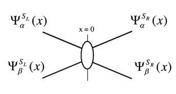
Figure 1: Quantum waveguide schematization of a two-band Josephson junction. Each branch represents a superconducting band, $\alpha$ or $\beta$, in the left ($S_{L}$) or right ($S_{R}$) electrode. The wave functions of supeconducting bands are given by $\Psi^{S_{L,R}}_{\alpha,\beta}(x)$. The node at $x=0$ represents the interface between the left and right superconducting banks.

II Model and Theory

We formulate a ballistic theory of the Josephson effect describing multiband superconducting junctions. The theory allows to consider an arbitrary number of bands, which are treated as network branches of an effective quantum waveguide model. The proposed approach could be applied to the $\mathrm{Mg}\mathrm{B}_{2}$ as well as the FeBS case. In order to develop the theory, hereafter we refer to the specific case of FeBS for which the $s_{++}$ and $s_{\pm}$ symmetries have been suggested. The Josephson effect in FeBS has been already studied by using a number of different methods burm2 ; burm1 ; golu ; nap ; moor ; da ; stan ; lin ; apos ; kosh ; berg ; ota ; erin ; park ; wu1 ; ng ; golu2 ; lind ; tsai ; chen2 . However, most of these studies, except few cases nap ; moor ; da , deal with the so-called hybrid Josephson junction in which the junction is formed by a conventional (s-wave) superconductor and a ($s_{\pm}$ or $s_{++}$) FeBS. We specialize here to the case of an all-FeBS coplanar Josephson junction, in which both the electrodes are FeBS materials (symmetric junction), as occurs for instance in grain boundary junctions. So far, several Josephson junctions using thin films have been fabricated seba ; dor ; dor2 ; schm ; lee ; kata1 ; kata2 ; sarn ; wu2 ; baro on bicrystal substrates (for a review on Fe-based Josephson junctions, see Ref.seidel and references therein) and thus a theoretical effort along this direction is needed.
Thus we consider a Josephson junction model in which the electrodes are two-band FeBS. To this end the junction is represented by a network of four one-dimensional branches connected to a single node point $x=0$ (see Fig. 1), $x$ being the coordinate along the propagation direction normal to the interface. Each superconducting branch represents the $i$-th band on the left or the right side of the junction, while the band wave function $\Psi_{i}=\theta(-x)\Psi^{S_{L}}_{i}(x)+\theta(x)\Psi^{S_{R}}_{i}(x)$, in the clean limit, obeys the equation

$$\left[\begin{array}[]{rl}&\hat{H}_{j}(x)\hskip 14.22636pt\Delta_{j}(x)\\ &\Delta^{*}_{j}(x)\hskip 14.22636pt-\hat{H}^{*}_{j}(x)\end{array}\right]\Psi_{j}=E\Psi_{j}$$ (3)

where $j\in\{\alpha,\beta\}$ is the band index, while

$$\Delta_{j}(x)=\Delta_{j}e^{i\varphi_{j}}\theta(-x)+\Delta_{j}e^{i(\varphi_{j}+\varphi)}\theta(x),$$ (4)

($\theta(x)=0$, for $x\leq 0$, $\theta(x)=1$ for $x>0$) are the two coexisting pair potentials. The operator $\hat{H}_{j}(x)$ represents the single particle Bogoliubov-de Gennes Hamiltonian in the two bands, which reads

$$\hat{H}_{j}(x)=-\frac{\hbar^{2}}{2m_{j}}\frac{\partial^{2}}{\partial x^{2}}-E_{F}.$$ (5)

In writing Eq. (4) we are neglecting the proximity effect and assuming that the inhomogeneous character of the gap in the junction is captured by choosing $\Delta_{\alpha}=\Delta_{\beta}=0$ just at the node (short junction). The two gap values $\Delta_{\alpha}$, $\Delta_{\beta}$, with $\Delta_{\alpha}<\Delta_{\beta}$, are assumed to be the same in the two superconductive leads. The quantity $\varphi$ is the gauge invariant phase difference between the two superconductive regions, $\varphi_{\alpha}$ and $\varphi_{\beta}$ the internal pair potential phases. In the case of $s_{\pm}$-wave gap model, $\varphi_{\beta}-\varphi_{\alpha}=\pi$ and the two gap have opposite sign, while in the standard two band model, with same sign gaps, $\varphi_{\beta}-\varphi_{\alpha}=0$. The quantities $m_{j}$ in Eq. (5) are the effective masses of quasiparticles in the $j$-th superconducting branch and are material-dependent quantities. We also introduce a single-particle node potential $U(x)$ which is different from zero only for $x=0$ and can be modeled as the usual Blonder-Tinkham-Klapwijk blond interface potential $U(x)=U_{0}\delta(x)$, even though this limiting assumption is not required to develop the theory. The node potential $U(x)$ allows the modeling of a FeBS/insulator/FeBS or FeBS/normal-metal/FeBS junction in which a normal scattering at the interface reduces the transparency of the junction. The junction barrier strength can be still characterized by introducing a Blonder-Tinkham-Klapwijk dimensionless parameter $Z=mU_{0}/(\hbar^{2}k_{F})$ ($m$ being the bare electron mass and $k_{F}^{2}=2mE_{F}/\hbar^{2}$) within the boundary conditions of the scattering problem. The modified boundary conditions used here (see Eqs.(22), (23)) account for band-sensitive scattering effects and have been already introduced in Ref. Romeo to describe the differential conductance of a normal-metal/FeBS junction; in the following we discuss their generalization to the Josephson junction case. The potentials $U(x)$ and $\Delta_{j}(x)$ are responsible for the normal scattering and the scattering of electrons into holes (Andreev scattering) at the interface, respectively. The four wave functions, $\Psi^{S_{L}}_{j}(x)$, $\Psi^{S_{R}}_{j}(x)$ ($j=\alpha,\beta$), one for each branch in the two electrodes, can be written in terms of the eigenstates of the local Hamiltonians as

$$\Psi^{S_{L}}_{j}(x)=\left[\begin{array}[]{rl}&u^{L}_{j}(x)\\ &v^{L}_{j}(x)\end{array}\right]=$$ (8)

$${a_{j}}\left(\begin{array}[]{rl}&v_{j}\\ &u_{j}e^{-i\varphi_{j}}\end{array}\right)e^{ip^{j}_{h}x}+b_{j}\left(\begin{array}[]{rl}&u_{j}\\ &v_{j}e^{-i\varphi_{j}}\end{array}\right)e^{-ip^{j}_{e}x},$$ (12)

for $x<0$ or

$$\Psi^{S_{R}}_{j}(x)=\left[\begin{array}[]{rl}&u^{R}_{j}(x)\\ &v^{R}_{j}(x)\end{array}\right]=$$ (15)

$$c_{j}\left(\begin{array}[]{rl}&u_{j}\\ &v_{j}e^{-i(\varphi_{j}+\varphi)}\end{array}\right)e^{ip^{j}_{e}x}+\ d_{j}\left(\begin{array}[]{rl}&v_{j}\\ &u_{j}e^{-i(\varphi_{j}+\varphi)}\end{array}\right)e^{-ip^{j}_{h}x},$$ (19)

for $x>0$. Here $u_{\alpha}$ and $v_{\alpha}$, and $u_{\beta}$ and $v_{\beta}$ are the Bogoliubov coefficients for the first and second band, respectively

$$u_{j}=\left[\frac{1}{2}\left(1+i\frac{\Omega_{j}}{E}\right)\right]^{1/2},v_{j}=\left[\frac{1}{2}\left(1-i\frac{\Omega_{j}}{E}\right)\right]^{1/2}$$

with $\Omega_{j}=\sqrt{\Delta_{j}(T)^{2}-E^{2}}$, $j\in\{\alpha,\beta\}$, while $T$ represents the temperature of the thermal bath. The wave vectors of the two bands

$${p^{j}_{e,h}}=\sqrt{r_{j}^{2}k_{F}^{2}\pm 2im_{j}\Omega_{j}/\hbar^{2}}$$

are well approximated by the expressions:

$$p^{\alpha}_{e,h}\simeq r_{\alpha}k_{F}\left(1\pm i\chi{\sqrt{1-E^{2}/{\Delta_{\alpha}}^{2}}}\right),$$ (21)

$$p^{\beta}_{e,h}\simeq r_{\beta}k_{F}\left(1\pm i\chi{\sqrt{{\Delta_{\beta}}^{2}/{\Delta_{\alpha}}^{2}-E^{2}/{\Delta_{\alpha}}^{2}}}\right),$$

which are valid under the assumptions $E_{F}\gg\Delta_{\beta}$, while the different signs $"+"$, $"-"$ refer to electronlike or holelike excitations respectively. The coefficient $r_{j}^{2}=m_{j}/m$ represents the effective mass of the $j$-th band measured in units of the bare electron mass $m$. In writing Eqs. (21) we have introduced the dimensionless factor $\chi=\Delta_{\alpha}(T)/2E_{F}$ or $\chi=\Delta_{\alpha}(T)/(k_{F}v_{F}\hbar)$, which represents the ratio between the Fermi wavelength $k_{F}^{-1}$ and the coherence length $\xi(T)\sim\hbar v_{F}/\Delta_{\alpha}(T)$. Its zero temperature value, $\chi_{0}$, can be also defined as $\chi_{0}=\Delta_{\alpha}(0)/(2E_{F})$. Since we are interested in localized subgap states, in Eq. (21) we assume $E<\Delta_{\alpha}(0)$, ensuring that the wave functions $\Psi^{S_{L}}_{j}(x)$, $\Psi^{S_{R}}_{j}(x)$ ($j=\alpha,\beta$) decay exponentially for $|x|\rightarrow\infty$.
The quasiparticle wave functions obey the generalized matching quantum waveguide conditions Romeo

$$\Psi^{S_{R}}_{\alpha}(0)=s_{\alpha}\Psi^{S_{L}}_{\alpha}(0),\qquad\Psi^{S_{R}}_{\beta}(0)=s_{\beta}\Psi^{S_{L}}_{\alpha}(0),\qquad\Psi^{S_{L}}_{\beta}(0)=s\Psi^{S_{L}}_{\alpha}(0)$$ (22)

$$\frac{\partial}{\partial x}\left[s_{\alpha}\frac{1}{r_{\alpha}^{2}}\Psi^{S_{R}}_{\alpha}+s_{\beta}\frac{1}{r_{\beta}^{2}}\Psi^{S_{R}}_{\beta}\right]_{x=0}-\frac{\partial}{\partial x}\left[\frac{1}{r_{\alpha}^{2}}\Psi^{S_{L}}_{\alpha}+s\frac{1}{r_{\beta}^{2}}\Psi^{S_{L}}_{\beta}\right]_{x=0}=2k_{F}Z\Psi^{S_{L}}_{\alpha}(0).$$ (23)

Equations (22) and (23) guarantee the conservation of the charge current at the node $x=0$ (quantum Kirchhoff’s law) and generalize the waveguide boundary conditions given in Ref. Romeo to the Josephson junction case. The three new parameters $s_{\alpha},s_{\beta},s$ characterize the interface and make the scattering and the current flow band-sensitive. Indeed, the overlap between the wave functions on different sides of the junction may favour scattering events towards a specific band, $\alpha$ or $\beta$. The existence of these ’band coupling parameters’ implies that a discontinuity of the wave functions may occur at the node ($x=0$) when at least one of the coupling parameters $s_{\alpha},s_{\beta},s$ is different from one. The meaning of this discontinuity has been discussed in Ref. [Romeo, ] in connection with the theory of PCARS in multiband superconductors. The physical meaning of the overlap parameters $s_{\alpha},s_{\beta},s$ can be easily understood observing that setting, for instance, $s_{\alpha}=0$ implies $\Psi^{S_{R}}_{\alpha}(0)=0$. Thus the wave function $\Psi^{S_{R}}_{\alpha}(x)$ presents a vanishing overlap at the interface with the remaining branch wave functions. As a consequence, in this case, the band $\alpha$ on the right side of the junction is excluded from the transport. The latter point can be further clarified by looking at the prefactor of the first term of Eq. (23), namely $s_{\alpha}(m_{\alpha}/m)^{-1}$, which governs the particle flow through the $\alpha$ band on the right side of the junction. Lowering $s_{\alpha}$ has the same effect of increasing $m_{\alpha}$, causing a lowering of the particles flux through the considered band. In the equal coupling case ($s_{\alpha}=s_{\beta}=s=1$) the partitioning of the current among different network branches is entirely governed by the bulk mass ratios $r_{j}$ and only weakly affected by the interface scattering potential strength $Z$. Thus the parameters $s_{\alpha},s_{\beta},s$ can be properly interpreted as overlap or coupling factors which define the fraction of current flowing through a specific band.
Eqs. (22)-(23) provide a linear system of equations for the eight unknown coefficients $a_{j}$, $b_{j}$, $c_{j}$, $d_{j}$ ($j\in\{\alpha,\beta\}$), appearing in the wave functions (see Appendix A). The bound state spectrum can be determined imposing the condition that this homogeneous system of equations has a nontrivial solution. Within the Andreev’s approximation, i.e. $p_{e}^{\alpha}\simeq p_{h}^{\alpha}\simeq r_{\alpha}k_{F}$ and $p_{e}^{\beta}\simeq p_{h}^{\beta}\simeq r_{\beta}k_{F}$, this critical condition is written as

$$-\frac{s_{\beta}^{2}(\epsilon^{2}-\gamma^{2})(1-\epsilon^{2}-2s_{\alpha}^{2}\epsilon^{2}-s_{\alpha}^{4}(\epsilon^{2}-1)+2s_{\alpha}^{2}\cos\varphi)}{r_{\alpha}^{2}}+$$

$$\frac{s^{2}(\epsilon^{2}-1)(2ss_{\beta}^{2}\epsilon^{2}+(s^{2}+s_{\beta}^{4})(\epsilon^{2}-\gamma^{2})-2ss_{\beta}^{2}\gamma^{2}\cos\varphi)}{r_{\beta}^{2}}+$$

$$\frac{2ss_{\beta}\sqrt{\epsilon^{2}-1}\sqrt{\epsilon^{2}-\gamma^{2}}\left(s((1+s_{\alpha}^{2})\epsilon^{2}-e^{i\delta}\gamma)+s_{\beta}^{2}((1+s_{\alpha}^{2})\epsilon^{2}-e^{i\delta}s_{\alpha}^{2}\gamma)-e^{i\delta}(ss_{\alpha}^{2}+s_{\beta}^{2})\gamma\cos\varphi\right)}{r_{\alpha}r_{\beta}}+$$

$$4s_{\beta}^{2}Z^{2}(\epsilon^{2}-1)(\epsilon^{2}-\gamma^{2})=0,$$ (24)

where $\delta=\varphi_{\beta}-\varphi_{\alpha}$, $\gamma=\Delta_{\beta}/\Delta_{\alpha}$ and $\epsilon=E/\Delta_{\alpha}(T)$. Choosing $\delta=0$ or $\delta=\pi$ reflects the internal pairing symmetry $s_{++}$ or $s_{\pm}$, respectively.

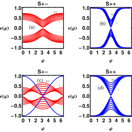
Figure 2: Bound states energy levels $E^{+}(\varphi)$ and $E^{-}(\varphi)$ (normalized to $\Delta_{\alpha}(T)$) calculated through Eq. (II). Panels (a), (c): $s_{\pm}$ symmetry. Panels (b), (d): $s_{++}$ symmetry. $Z$ and $\gamma$ have been fixed to $Z=0.03$ and $\gamma=3$, the various curves are obtained by letting parameter $s_{\alpha}$ to vary in the range $(0.3,1)$ in steps of $0.1$, while $s_{\beta}=s=1$. Panels (a) and (b): $r_{\alpha}=1.8$, $r_{\beta}=1$. Panels (c) and (d): $r_{\alpha}=1$, $r_{\beta}=1.8$, the blue line curve in panel (c) is the Andreev level of a conventional s-wave junction with $r_{j}Z=0.03$.

Two sets of energy levels $E^{+}(\varphi)$ and $E^{-}(\varphi)$ are found in solving Eq. (II), which correspond to electronlike and holelike quasiparticles, respectively. One finds that the Andreev bound states never appear beyond $\Delta_{\alpha}$. When $s_{\alpha}=s_{\beta}=s=1$, in the two limits $r_{\alpha}\rightarrow\infty$ or $r_{\beta}\rightarrow\infty$ (exclusion of the $\alpha$ or $\beta$ band respectively) Eq. (II) provides the well known s-wave result $E=E_{B}=\Delta_{j}\sqrt{(\cos^{2}(\varphi/2)+Z_{j}^{2})/(1+Z_{j}^{2})}$, with $Z_{j}=r_{j}Z$ nota-Zj , $j$ being $\alpha$ or $\beta$ (see Fig. 2 (c)).
In Fig. 2 we show Andreev bound states spectra computed using Eq. (II). Once the mass ratios $r_{j}$ have been fixed, different Josephson couplings can be obtained depending on the kind of the order parameter symmetry and on the choice of the overlap factors. To better explain this point, we present different curves obtained by letting the parameter $s_{\alpha}$ to vary in the range $(0.3,1)$ in steps of $0.1$ while $s_{\beta}=s=1$. This choice of the overlap factors corresponds to weaken progressively the coupling of the band $\Psi^{S_{R}}_{\alpha}$ from the remaining bands. Panels (a) and (b) ($r_{\alpha}=1.8$, $r_{\beta}=1$) show a generalized lowering of the levels toward the zero energy state in the case of $s_{\pm}$ symmetry (panel (a)), which is absent in the case of $s_{++}$ symmetry (panel (b)) and represents the main difference between the two symmetries in this case. A further difference is illustrated in panels (c) and (d) ($r_{\alpha}=1$, $r_{\beta}=1.8$). In the case of $s_{\pm}$ symmetry (panel (c)) the energy levels undergo a gradual concavity change as the parameter $s_{\alpha}$ is decreased. This concavity change is responsible for a $\pi$-shift in the current-phase relation, which is not observed in the $s_{++}$ case (Fig. 2(d)). Thus, as also observed elsewhere nap , a $0-\pi$ transition may be a distinctive signature of the $s_{\pm}$ symmetry. This point will be further explained in Section IV, where the current-phase relations and the temperature dependence of the maximum Josephson current will be presented.

III Josephson current

The Josephson current flowing through the junction could be directly computed from the Andreev bound states according to the formula benakk :

$$I_{J}(\varphi)\approx-\frac{2e}{\hbar}\frac{dE^{+}(\varphi)}{d\varphi}\tanh\Big{[}\frac{E^{+}(\varphi)}{2k_{B}T}\Big{]}.$$ (25)

Due to the special character of the bound state of a multiband junction, in the following we will characterize the Josephson current by using a field theory formalism in second quantization. We verified that the latter procedure provides results consistent with those obtained using Eq. (25).
The Cooper pair charge flow $\bar{J}_{ch}$ through the junction can be computed as quantum-statistical average of the current density operator according to the expression $\bar{J}_{ch}=\sum_{j,\sigma}\langle\hat{\psi}_{j\sigma}^{{\dagger}}\check{\mathcal{J}}_{j}\hat{\psi}_{j\sigma}\rangle$, where $\check{\mathcal{J}}_{j}=\frac{i\hbar|e|}{2m_{j}}(\overrightarrow{\partial}_{x}-\overleftarrow{\partial}_{x})$ represents the first-quantization band operator nota_diff_op . The second quantized fields $\hat{\psi}_{j\sigma}$ ($\hat{\psi}_{j\sigma}^{{\dagger}}$) represent the annihilation (creation) operators of a spin $\sigma$ electron in the $j$-th band and obey a fermionic algebra. These fields provide an appropriate basis in the absence of superconducting correlations. However, when the superconductivity is established, $\hat{\psi}_{j\sigma}$ are not eigenfields of the problem and, for this reason, the Nambu representation can be conveniently used $\Psi(x)=\sum_{j\in\{\alpha,\beta\}}|j\rangle\otimes(\hat{\psi}_{j\uparrow},\hat{\psi}^{{\dagger}}_{j\downarrow})^{t}$. The Nambu field $\Psi(x)$ is a non-local quantity describing particle-hole excitations in different network branches and can be expanded in eigenfields of the Hamiltonian problem on the network. Limiting the expansion to the eigenfields $\hat{\gamma}_{\sigma}$ describing the low-energy (sub-gap) states with energy $\pm E_{B}\in[-\Delta_{\alpha},\Delta_{\alpha}]$, we get:

$$\Psi(x)\approx\hat{\gamma}_{\uparrow}e^{-iE_{B}t/\hbar}\psi_{B}(x)+\hat{\gamma}^{{\dagger}}_{\downarrow}e^{iE_{B}t/\hbar}\tilde{\psi}_{B}(x),$$ (26)

where $\psi_{B}(x)=\theta(-x)\psi^{(L)}_{B}(x)+\theta(x)\psi^{(R)}_{B}(x)$ is the wave function of the electron-like bound state having energy eigenvalue $E_{B}>0$, while $\tilde{\psi}_{B}(x)=[\sum_{j}|j\rangle\langle j|\otimes i\hat{\sigma}_{y}\mathcal{C}]\psi_{B}(x)$ represents its time-reversed state associated with a hole-like state with energy $-E_{B}$. The electron-like bound state is localized at the interface and extends over all the waveguide branches. Thus eigenstates of the local branch Hamiltonians can be used to expand $\psi_{B}(x)$, using the following decomposition:

$$\psi^{(\nu)}_{B}(x)=\sum_{j\in\{\alpha,\beta\}}|j\rangle\otimes\left[\begin{array}[]{rl}&u^{\nu}_{j}(x)\\ &v^{\nu}_{j}(x)\end{array}\right],$$ (29)

with $\nu\in[L,R]$ an index identifying the left ($x<0$) or right ($x>0$) side of the junction. Once $\Psi(x)$ has been expanded in eigenfields $\hat{\gamma}_{\sigma}$ it is possible to recognize the fermionic fields $\hat{\psi}_{j\uparrow}$ in the expression:

$$\hat{\psi}_{j\uparrow}\approx\hat{\gamma}_{\uparrow}e^{-iE_{B}t/\hbar}u_{j}(x)-\hat{\gamma}^{{\dagger}}_{\downarrow}e^{iE_{B}t/\hbar}v_{j}(x)^{\ast},$$ (30)

with $u_{j}(x)=\theta(-x)u^{L}_{j}(x)+\theta(x)u^{R}_{j}(x)$ and analogously for $v_{j}(x)$. Substituting Equation (30) in the expression for $\bar{J}_{ch}$, in the absence of spin-sensitive potentials nota_current , we obtain ($x>0$):

$$\bar{J}_{ch} = \frac{-2|e|\hbar}{m}\sum_{j}r_{j}^{-2}\Bigl{\{}\mathrm{Im}[u^{R}_{j}(x)^{\ast}\partial_{x}u^{R}_{j}(x)]f(E_{B})+$$ (31)

$$+ \mathrm{Im}[v^{R}_{j}(x)\partial_{x}v^{R}_{j}(x)^{\ast}](1-f(E_{B}))\Bigl{\}},$$

where we explicitly used the thermal equilibrium averages $\langle\hat{\gamma}^{{\dagger}}_{\sigma}\hat{\gamma}_{\sigma}\rangle=f(E_{B})$ and $\langle\hat{\gamma}_{\sigma}\hat{\gamma}^{{\dagger}}_{\sigma}\rangle=1-f(E_{B})$. Due to the current conservation we have the freedom to evaluate the current in $x=0^{+}$, and thus starting from Eq. (31) we get ($e=-|e|$) nota_current2 :

$$\bar{J}_{ch}=-2ev_{F}\sum_{j}\frac{u_{j}v_{j}}{r_{j}}\left(|c_{j}|^{2}-|d_{j}|^{2}\right)\tanh\left[\frac{E_{B}}{2k_{B}T}\right],$$ (32)

where the coefficients $c_{j}$ and $d_{j}$ are calculated at the energy $E_{B}=\epsilon_{B}(\varphi)\Delta_{\alpha}(T)$, while $\epsilon_{B}(\varphi)$ is solution of Eq. (II). It’s worth mentioning here that the Fermi velocity in the $i$-th band is given by $v^{(i)}_{F}=v_{F}/r_{i}$, while the quantity $v_{F}=\hbar k_{F}/m$ is just used as velocity unit. Equation (32) is one of the main results of this work and generalizes the expression found in Ref. [furusaki, ] to the multi-band case.
Equation (32), complemented by the coefficients $c_{j}$ and $d_{j}$ derived following the procedure sketched in Appendix A, allows to obtain the current-phase relation of the junction. In deriving the scattering coefficients $a_{j}$, $b_{j}$, $c_{j}$, $d_{j}$ ($j\in\{\alpha,\beta\}$), Eqs. (22)-(23) have to be complemented by the normalization condition, $\int^{\infty}_{-\infty}dx\psi_{B}(x)^{{\dagger}}\psi_{B}(x)=1$, of the bound state wave function $\psi_{B}(x)$: $\sum_{j=\alpha,\beta}\int_{-\infty}^{0}[|u^{L}_{j}(x)|^{2}+|v^{L}_{j}(x)|^{2}]dx+\sum_{j=\alpha,\beta}\int_{0}^{+\infty}[|u^{R}_{j}(x)|^{2}+|v^{R}_{j}(x)|^{2}]dx=1$. The normalization condition can be satisfied only considering an imaginary part in the expressions of the quasiparticle momenta $p^{j}_{e}$ and $p^{j}_{h}$. This accounts for the localized nature of the bound state whose wave function contains decaying exponentials of the type $\sim\exp[\pm\chi r_{\alpha}k_{F}\sqrt{1-(E_{B}/\Delta_{\alpha})^{2}}x]$ and $\sim\exp[\pm\chi r_{\beta}k_{F}\sqrt{\gamma^{2}-(E_{B}/\Delta_{\alpha})^{2}}x]$, the decay length being comparable with the coherence length $\xi(T)\sim\hbar v_{F}/\Delta_{\alpha}(T)$. Due to the different decay lengths characterizing the bound state wave function, $|E_{B}|$ cannot exceed $\Delta_{\alpha}$. Indeed, assuming $E_{B}>\Delta_{\alpha}$, the quantum state is no more localized and its wave function $\psi_{B}(x)$ is not normalizable. The above arguments explains why the bound state energy $E_{B}$ cannot exceed the minimum value among the superconducting gaps describing the multiband junction. This latter aspect suggests that the performances of a multiband Josephson junction can be strongly affected by disorder effects and inhomogeneities.

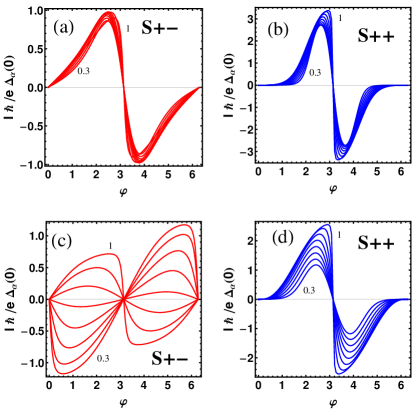
Figure 3: Current-phase relations at $T=0.001T_{c}$. Panels (a) and (c): $s_{\pm}$ symmetry. Panels (b) and (d): $s_{++}$ symmetry. Parameters are the same of the corresponding panels in Fig. 2; (a) and (b): $Z=0.03$, $\gamma=3$, $r_{1}=1.8$, $r_{2}=1$; (c) and (d): $Z=0.03$, $\gamma=3$, $r_{1}=1$, $r_{2}=1.8$. The value of $\chi_{0}$ has been set to $\chi_{0}=0.01$. The various curves are obtained by letting parameter $s_{\alpha}$ to vary in the range $(0.3,1)$ in steps of $0.1$, while $s_{\beta}=s=1$.

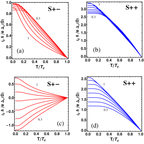
Figure 4: Josephson critical current as a function of the reduced temperature $T/T_{c}$. Panels (a) and (c): $s_{\pm}$ symmetry. Panels (b) and (d): $s_{++}$ symmetry. Parameters are the same of the corresponding panels in Fig. 2: $Z=0.01$, $\gamma=3$. The value of $\chi_{0}$ has been set to $\chi_{0}=0.01$. (a) and (b) $r_{1}=1.8$, $r_{2}=1$. (c) and (d), $r_{1}=1$, $r_{2}=1.8$. The critical current is in units of $e\Delta_{\alpha}(0)/\hbar$. The various curves are obtained by letting parameter $s_{\alpha}$ to vary in the range $(0.3,1)$ in steps of $0.1$, while $s_{\beta}=s=1$.

IV Numerical Results

In this section we provides specific examples of current-phase relation derived through Eq. (32). We assume that the temperature dependence of both gaps $\Delta_{j}$ ($j=\alpha,\beta$) is given by $\Delta_{j}(T)=\Delta_{j}(0)\tanh\left(1.74\sqrt{T_{c}/T-1}\right)$, where $T_{c}$ is the critical temperature of the superconducting transition. We also assume the validity of the BCS ratio $\Delta_{\alpha}(0)/k_{B}T_{c}=1.76$ between the critical temperature and the zero temperature pair potential. Under these assumptions, the parameter $\gamma=\Delta_{\beta}/\Delta_{\alpha}$ does not depend on the temperature. Note that the quantity $\chi_{0}$ has been assigned the value 0.01 in the calculations but that the results do not depend on the specific value of $\chi_{0}$, provided that $\chi_{0}\ll 1$.
In Figure 3 we present the current-phase relation of two junction configurations whose bound states energy has been shown in Fig. 2. In particular, in panels (a) and (b), we report the current-phase relation computed for the $s_{\pm}$ and the $s_{++}$ symmetry, respectively, setting the model parameters as follows: $Z=0.03$, $\gamma=3$, $r_{1}=1.8$, $r_{2}=1$. The different curves are obtained by letting the parameter $s_{\alpha}$ to vary in the range $(0.3,1)$ in steps of $0.1$, while $s_{\beta}=s=1$. One notices a strong suppression of the Josephson current in the $s_{\pm}$ symmetry (panel (a)) compared to the $s_{++}$ case (panel (b)). This phenomenon originates from the destructive interference effects of quasiparticles experiencing two opposite gap signs. The destructive interference lowers the Andreev reflection probability such that, in perfectly symmetric junctions (i.e. $r_{\alpha}=r_{\beta}$, $s_{\alpha}=s_{\beta}=s=1$), the current exactly vanishes. Thus $s_{++}$ Josephson junctions exhibit greater critical current values ($I_{c}(T\rightarrow 0)\sim e\Delta_{\beta}/\hbar$) compared to those expected for the $s_{\pm}$ case ($I_{c}(T\rightarrow 0)\sim e\Delta_{\alpha}/\hbar$). On the other hand, the peculiar functional form of the current-phase relation of the $s_{++}$ symmetry (panel (b)) indicates a certain fragility of this junction against bias current fluctuations. Indeed, a small bias fluctuation (less than few percent of the critical current) can cause, at low bias, a relevant phase fluctuation. This stochastic phase jump may represent a relevant source of voltage fluctuation across the junction which can also drive the system towards an ohmic regime.
Figures 3(c) and 3(d) are obtained by setting $r_{\alpha}=1.8$ and $r_{\beta}=1$, while maintaining the remaining parameters at the same values fixed in the upper panels of Figure 3. In particular, panel (c) shows an $s_{\pm}$ current-phase relation that, as also evident from the Andreev levels (Figure 2 (c)), undergoes a $\pi$-shift as the $s_{\alpha}$ parameter varies between the values $0.3$ and $1$. The $\pi$-shift is absent in panel (d) where the current-phase curve is shown for the $s_{++}$ symmetry. A $\pi$-junction presents a free energy $F(\varphi)=\Phi_{0}/2\pi\int_{0}^{\varphi}d\theta I(\theta)$ minimum at $\varphi=\pi$ rather than at $\varphi=0$. The existence of $\pi$-shifted junctions can be experimentally proved employing SQUID’s measurements.
While the current-phase relation cannot be simply measured, the measurement of the temperature dependence of the junction critical current is relatively easier. A comparison with the experiments of this dependence represents very often an important tool contributing to identifying the nature of the superconducting pairing. Thus, in order to compare our results with the experimental findings, we have derived the temperature dependence of the maximum Josephson current (critical current). Figure 4 shows the temperature dependence of the critical current calculated for the $s_{\pm}$- ((a) and (c)) and $s_{++}$-symmetry ((b) and (d)) by setting the model parameters as done in Figs. 2 and 3. Negative critical current values, like those presented in panel (c), indicates a $\pi$-shifted Josephson junction. A common feature of all the panels in Figure 4 is the violation of the Ambegaokar-Baratoff relation, which is usually reported in multiband S/I/S Josephson junctions ambegaokar_baratoff-violation . The entity of such violation depends on the junction parameters and is more pronounced for the $s_{\pm}$ symmetry (see panels (a) and (c)), where the critical current vs temperature curves develop a peculiar positive curvature. Panels (b) and (d) are described by a deformed Ambegaokar-Baratoff relation and suggest that a $\pi$ junction cannot be observed for the $s_{++}$ symmetry. In this respect we observe that the $0-\pi$ transition reported in the present work (see Figure 3(c) and 4(c)) is the result of a different mechanism compared to the one described in Ref. nap . There the transition originates from the competition of two Andreev bound states carrying opposite current. As the temperature is lowered the state with higher energy eigenvalue is progressively excluded from the transport and a sign reversal of the critical current is observed. Here we predict the presence of a single electron-like bound state and thus a temperature activated $0-\pi$ transition cannot be observed as an intrinsic effect. However, direct tunneling ($\alpha\rightarrow\alpha$ or $\beta\rightarrow\beta$) and crossed tunneling ($\alpha\rightarrow\beta$ or $\beta\rightarrow\alpha$) effects provide supercurrent contribution with opposite sign and thus, depending on the relative strength of these contributions, a $\pi$-junction can be formed only assuming the $s_{\pm}$ symmetry. The relative strength of the direct and crossed tunneling contributions is controlled in the model by the overlap parameters $s_{\alpha}$, $s_{\beta}$, and $s$ which are characteristic of the interface. According to these arguments, a $0-\pi$ transition can occur by varying at least one overlap parameter. This can be done in different ways: (i) changing the temperature can induce a lattice deformation at the interface which is relevant in determining the overlap parameters; (ii) experiments performed under controllable pressure or strain allow to control lattice distortion and thus the overlap parameters. Both the methods (i) and (ii) can be used to induce the $0-\pi$ transition in multiband Josephson junctions. The mechanism of formation of a $\pi$-junction described above can be also recovered in the framework of a semiclassical theory of the $s_{\pm}/I/s_{\pm}$ Josephson junction as developed in Ref. deluca2013 .

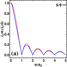
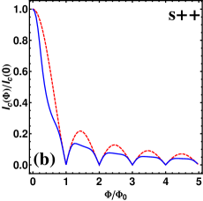
Figure 5: Normalized critical current $I_{c}(\Phi)/I_{c}(0)$ as a function of the applied magnetic flux $\Phi/\Phi_{0}$ computed for the $s_{\pm}$ (panel (a)) and the $s_{++}$ symmetry (panel (b)). Parameters are the same of the corresponding panels in Fig. 3: $Z=0.03$, $\gamma=3$, $r_{1}=1.8$, $r_{2}=1$, $s_{\alpha}=s_{\beta}=s=1$, $\chi_{0}=0.01$ and $T=0.001T_{c}$. The dashed curve in each panel represents the Fraunhofer pattern for comparison.

However, as clearly evidenced in Figs. 3(a)-(b), the $0-\pi$ transition is strongly affected by the bands effective mass and can remain unobserved also for an $s_{\pm}$ junction. Under this condition, the magnetic response of the system (see Appendix B for details) provides an indirect probe of the harmonic content of the current-phase relation and can help in discriminating the pairing symmetry of the junction. In particular, the zero-field critical current $I_{c}(0)$ of the $s_{++}$ case (see Fig. 3(b)) is greater than the corresponding value obtained for the $s_{\pm}$ case (see Fig. 3(a)). As a consequence, one expects that the harmonic content of the current-phase relation of the $s_{++}$ case strongly affects the low-field magnetic diffraction pattern of the junction. On the other hand, for the $s_{\pm}$ case, the high harmonic contribution is expected to be less important due to the lower value of zero-field critical current. The above arguments are confirmed by Fig. 5 where the normalized critical current $I_{c}(\Phi)/I_{c}(0)$ is studied as a function of the applied magnetic flux $\Phi/\Phi_{0}$ (normalized to the flux quantum $\Phi_{0}$) for the $s_{\pm}$ (panel (a)) and the $s_{++}$ (panel (b)) symmetry, while the model parameters are fixed as done for the corresponding panels in Fig. 3. Interestingly, the $s_{++}$ Josephson junction evidences a critical current halving already for flux values of $\sim 0.4\Phi_{0}$, while the critical current of the $s_{\pm}$ case is less sensitive to magnetic field effects.

V Conclusions

We have formulated a minimal model of the dc Josephson effect for multiband superconductors based on the quantum waveguide approach. The method is based on the analogy between multiband superconductors and multibranch networks recently suggested in Ref. Araujo . Accordingly, the subgap bound states wave functions (electron- and hole-like), relevant in describing the quantum transport within the short junction limit, are decomposed using the eigenstates of local branch Hamiltonians and the coefficients of such a decomposition are found imposing generalized boundary conditions on the wave functions. The boundary conditions, never used before for this problem, are direct generalization of those used in Ref. Romeo and incorporate a local scattering potential at the interface ($Z$ parameter) and band overlap factors $s_{\alpha}$, $s_{\beta}$, and $s$ which define the weight of each band in the quasiparticles transport. This provides an effective parametrization of the interface effects allowing to describe Josephson junctions ranging from the metallic ($Z\ll 1$) to the tunnel limit ($Z\gg 1$). The bulk properties of the superconducting bands are introduced using different effective masses ($r_{j}$ parameters) which can be determined by complementary experiments. We have solved the scattering problem and we have determined the Andreev bound states spectrum and the normalized eigenfunctions. The Josephson current flowing through the junction has been computed using a second quantization approach which correctly reproduces results obtained using the phase derivative of the Andreev bound states spectrum formula. The second quantization method used in the derivation of the Josephson current generalizes the result presented in Ref. furusaki for a single band superconductor to the multiband case and represents one of the main results of this work. To provide a specific and relevant application of the theory, we have focused our treatment on FeBS-FeBS tunnel junctions. In particular, we have derived the current-phase relations and the critical currents of symmetric FeBS junctions modeled as superconducting systems with two relevant bands. We have analyzed $s_{++}$ and $s_{\pm}$ symmetries of the FeBS and we have shown that a $\pi$-junction can be observed only for $s_{\pm}$ symmetry and under appropriate interface conditions, which are carefully discussed in the text. Further peculiar aspects of FeBS-FeBS tunnel junctions are also discussed. The above findings are relevant for the Josephson effect theory in multiband systems and can contribute to the current debate about the order parameter symmetry of iron-based materials.

Appendix A Determination of the scattering coefficients

The matching conditions Eqs. (22)-(23) provide the linear homogeneous system $\mathbf{M}\cdot\mathbf{X}=0$, where $\mathbf{X}=(a_{\alpha},...,d_{\alpha},a_{\beta},...,d_{\beta})^{t}$ and $\mathbf{M}$ is the following matrix

$$\left(\begin{array}[]{cccccccc}s_{\alpha}v_{\alpha}&s_{\alpha}u_{\alpha}&-u_{\alpha}&-v_{\alpha}&0&0&0&0\\ s_{\alpha}u_{\alpha}&s_{\alpha}v_{\alpha}&-e^{-i\varphi}v_{\alpha}&-e^{-i\varphi}u_{\alpha}&0&0&0&0\\ 0&0&0&0&s_{\beta}v_{\beta}&s_{\beta}u_{\beta}&-u_{\beta}&-v_{\beta}\\ 0&0&0&0&e^{-i\delta}s_{\beta}u_{\beta}&e^{-i\delta}s_{\beta}v_{\beta}&-e^{-i(\delta+\varphi)}v_{\beta}&-e^{-i(\delta+\varphi)}u_{\beta}\\ sv_{\alpha}&su_{\alpha}&0&0&0&0&-u_{\beta}&-v_{\beta}\\ su_{\alpha}&sv_{\alpha}&0&0&0&0&-e^{-i(\delta+\varphi)}v_{\beta}&-e^{-i(\delta+\varphi)}u_{\beta}\\ -\frac{v_{\alpha}(i+2r_{\alpha}Z)}{r_{\alpha}}&\frac{u_{\alpha}(i-2r_{\alpha}Z)}{r_{\alpha}}&\frac{is_{\alpha}u_{\alpha}}{r_{\alpha}}&-\frac{is_{\alpha}v_{\alpha}}{r_{\alpha}}&-\frac{isv_{\beta}}{r_{\beta}}&\frac{isu_{\beta}}{r_{\beta}}&\frac{is_{\beta}u_{\beta}}{r_{\beta}}&-\frac{is_{\beta}v_{\beta}}{r_{\beta}}\\ -\frac{u_{\alpha}(i+2r_{\alpha}Z)}{r_{\alpha}}&\frac{v_{\alpha}(i-2r_{\alpha}Z)}{r_{\alpha}}&\frac{ie^{-i\varphi}s_{\alpha}v_{\alpha}}{r_{\alpha}}&-\frac{ie^{-i\varphi}s_{\alpha}u_{\alpha}}{r_{\alpha}}&-\frac{ie^{-i\delta}su_{\beta}}{r_{\beta}}&\frac{ie^{-i\delta}sv_{\beta}}{r_{\beta}}&\frac{ie^{-i(\delta+\varphi)}s_{\beta}v_{\beta}}{r_{\beta}}&-\frac{ie^{-i(\delta+\varphi)}s_{\beta}u_{\beta}}{r_{\beta}}\\ \end{array}\right).$$ (33)

The homogeneous system admits non-trivial solution provided that the condition $det(\mathbf{M})=0$ (Eq. (II) of the main text) is fulfilled. Since $\mathbf{M}$ is not a maximal rank matrix, the normalization condition of the bound state wave function provides a further condition to determine the coefficients vector $\mathbf{X}$.

Appendix B Magnetic field dependence of the critical current

We describe the response of a Josephson junction under the application of a sufficiently weak external magnetic field $\vec{H}=H\hat{z}$ parallel to the $z$-axis. We explicitly assume the small junction limit in which the transverse dimension $L$ of the junction (parallel to the $y$-axis) is comparable or smaller than the Josephson penetration length $\lambda_{j}$ ($L\lesssim\lambda_{j}$) barone-book . The junction region, located at $x=0$, presents a reduced pairing potential and thus experiences the maximum magnetic field value, while inside the electrodes the polarizing effect of the field is effectively screened by supercurrents. Due to this, the spatial dependence of the magnetic field is given by $\vec{H}=H\hat{z}\exp(-|x|/\lambda)$. Since we are interested in the bulk effect of $\vec{H}$, observing that $\int_{-\infty}^{\infty}\vec{H}\cdot\hat{z}dx=2\lambda H$, we can approximate the spatial dependence of the field according to the expression $\vec{H}=\hat{z}\frac{\Phi}{L}\delta(x)$, where we introduced the magnetic flux $\Phi=2\lambda LH$ induced by the external field and the Dirac delta function $\delta(x)$. The magnetic field $\vec{H}=\vec{\nabla}\times\vec{A}$ can be expressed in terms of the vector potential $\vec{A}=(-\frac{\Phi y}{L}\delta(x),0,0)$ which is not affected by self-fields in the considered limit. Assuming that the Zeeman term is effectively screened in the bulk of the electrodes, the presence of $\vec{H}$ affects the BdG branch Hamiltonian $H_{BdG}^{(j)}$ (Eq. 3) only through the substitution $\hat{p}_{x}\rightarrow\hat{p}_{x}-eA_{x}$. The vector potential $A_{x}$ can be gauged away by means of the unitary transformation

$$U=\exp(i\pi\frac{\Phi}{\Phi_{0}}\frac{y}{L}\theta(x)\hat{\sigma}_{z}),$$ (34)

with $\hat{\sigma}_{z}$ a Pauli matrix acting on the particle-hole space and $\Phi_{0}=h/(2|e|)$ the elementary flux quantum. The transformed branch Hamiltonian $\widetilde{H}^{(j)}_{BdG}=U^{{\dagger}}H^{(j)}_{BdG}U$ under the action of $U$ can be obtained with the following substitutions:

$$U^{\ast}_{11}\hat{H}_{j}(x;A_{x})U_{11}\rightarrow-\frac{\hbar^{2}\partial^{2}_{x}}{2m_{j}}$$

$$-U^{\ast}_{22}\hat{H}^{\ast}_{j}(x;A_{x})U_{22}\rightarrow\frac{\hbar^{2}\partial^{2}_{x}}{2m_{j}}$$

$$\Delta_{j}(x)U^{\ast}_{11}U_{22}\rightarrow\widetilde{\Delta}_{j}(x),$$ (35)

while the BdG state associated to $\widetilde{H}^{(j)}_{BdG}$ is given by $\widetilde{\Psi}_{j}=U^{{\dagger}}\Psi_{j}$. The pair potential $\widetilde{\Delta}_{j}(x)$ takes the same mathematical structure of the one presented in Eq. (4), the only action of the unitary transformation being the substitution of the phase difference $\varphi$ with $\widetilde{\varphi}=\varphi-2\pi\frac{\Phi}{\Phi_{0}}\frac{y}{L}$. As a consequence the phase difference between the two sides of the junction is modulated along the junction and this modulation is the source of the magnetic diffraction pattern affecting the critical current of the junction. Under our assumptions, the $y$-dependence of the pair potential is adiabatic compared to the microscopic scale of the problem. This statement can be rigorously proved using the two-scale perturbation theory strogatz . In particular the wave vector, $q=\frac{2\pi}{L}\frac{\Phi}{\Phi_{0}}$, modulating the superconducting phase is much smaller than the Fermi wave vectors $r_{j}k_{F}$ and thus the phase modulation along the $y$-direction enters only parametrically in the one dimensional problem described in the main text. The validity of these arguments also requires that the Cooper pairs tunneling with normal incidence represents the dominant microscopic process and thus the energy associated with transverse modes is negligible compared to the Fermi energy. When the energy of the transverse modes becomes relevant (e.g. for very short junctions with $L\ll\lambda$) on the Fermi energy scale, a full treatment of the transverse degrees of freedom is required. Hereafter, we focus our attention on the case of adiabatic phase variation of $\widetilde{\varphi}$ along the transverse dimension of the junction. Under this assumption, once the current-phase relation $I_{J}(\varphi)$ has been obtained according to the procedure given in the main text, the magnetic field dependence of the critical current of the junction is obtained according to the formula:

$$I_{c}(\Phi)=\max_{\varphi\in[0,2\pi]}\int_{-L/2}^{L/2}\frac{dy}{L}I_{J}\left(\varphi-2\pi\frac{\Phi}{\Phi_{0}}\frac{y}{L}\right),$$ (36)

where the current-phase relation presents a parametric dependence on $y$. A further progress can be done observing that the current-phase relation is an odd function of the phase difference and thus it can be written as $I_{J}(\varphi)=\sum_{n=0}^{\infty}a_{n}\sin(n\varphi)$. As a consequence, Eq. (36) takes the form:

$$I_{c}(\Phi)=\max_{\varphi\in[0,2\pi]}\sum_{n=0}^{\infty}a_{n}\sin(n\varphi)\frac{\sin(n\frac{\pi\Phi}{\Phi_{0}})}{n\frac{\pi\Phi}{\Phi_{0}}},$$ (37)

where the coefficients $a_{n}$ can be directly extracted by $I_{J}(\varphi)$ using the relation:

$$a_{n}=\frac{1}{\pi}\int_{0}^{2\pi}I_{J}(\varphi)\sin(n\varphi)d\varphi,$$ (38)

where we explicitly used the orthogonality condition $\int_{0}^{2\pi}\sin(n\varphi)\sin(m\varphi)d\varphi=\pi\delta_{n,m}$. Equation (37) provides the Fraunhofer diffraction pattern,

$$I_{c}(\Phi)/I_{c}(0)=\Bigl{|}\frac{\sin(\frac{\pi\Phi}{\Phi_{0}})}{\frac{\pi\Phi}{\Phi_{0}}}\Bigl{|},$$

when a single-harmonic current-phase dependence $I_{J}(\varphi)=a_{1}\sin(\varphi)$ is considered, while deviations are expected if the high-harmonic contribution is not negligible. For the above reasons, the magnetic diffraction pattern $I_{c}(\Phi)$ is an indirect probe of the harmonic content of the current-phase relation of the junction. Our treatment of the magnetic field effects on the junction justifies the validity of the approach proposed in Refs. goldobin ; sperstad and the classical argument given in Ref. barone-book .

References

- (1) H. Suhl, B. T. Matthias, and L. R. Walker, Phys. Rev. Lett. 3, 552 (1959); V. A. Moskalenko, Fiz. Met. Metalloved. 8, 503 (1959).
- (2) J. Bardeen, L. N. Cooper, J. R. Schrieffer, Phys. Rev. 108, 1175 (1957).
- (3) J. Nagamatsu, N. Nakagawa, T. Muranaka, Y. Zenitani, and J. Akimitsu, Nature (London) 410, 63 (2001).
- (4) Y. Kamihara, T. Watanabe, M. Hirano and H. Hosono, J. Am. Chem. Soc. 130, 3296 (2008).
- (5) G. R. Stewart, Rev. Mod. Phys. 83, 1589 (2011).
- (6) F. Giubileo, D. Roditchev, W. Sacks, R. Lamy, D. X. Thanh, J. Klein, S. Miraglia, D. Fruchart, J. Marcus, Ph. Monod, Phys. Rev. Lett. 87, 177008 (2001).
- (7) I. I. Mazin, D. J. Singh, M. D. Johannes, and M. H. Du, Phys. Rev. Lett. 101, 057003 (2008); K. Kuroki, S. Onari, R. Arita, H. Usui, Y. Tanaka, H. Kontani, H. Aoki, Phys. Rev. Lett. 101, 087004 (2008).
- (8) R. S. Gonnelli, D. Daghero, G. A. Ummarino, A. Calzolari, M. Tortello, V. A. Stepanov, N. D. Zhigadlo, K. Rogacki, J. Karpinski, F. Bernardini, and S. Massidda, Phys. Rev. Lett. 97, 037001 (2006).
- (9) D. Daghero, M. Tortello, G. A. Ummarino and R. S. Gonnelli, Rep. Prog. Phys. 74, 124509 (2011).
- (10) W. K. Park, J. L. Sarrao, J. D. Thompson, and L. H. Greene, Phys. Rev. Lett. 100, 177001 (2008).
- (11) S. Kashiwaya, Y. Tanaka, M. Koyanagi, H. Takashima, and K. Kajimura, Phys. Rev. B 51, 1350 (1995).
- (12) T. Y. Chen, Z. Tesanovic, R. H. Liu, X. H. Chen, and C. L. Chien, Nature (London) 453, 1224 (2008).
- (13) X. Lu, W. K. Park, H. Q. Yuan, G. F. Chen, G. L. Luo, N. L. Wang, A. S. Sefat, M. A. McGuire, R. Jin, B. C. Sales, D. Mandrus, J. Gillett, S. E. Sebastian, and L. H. Greene, Supercond. Sci. Technol. 23, 054009 (2010).
- (14) E. Il’ichev, M. Grajcar, R. Hlubina, R. P. J. IJsselsteijn, H. E. Hoenig, H.-G. Meyer, A. Golubov, M. H. S. Amin, A. M. Zagoskin, A. N. Omelyanchouk, and M. Yu. Kupriyanov, Phys. Rev. Lett. 86, 5369 (2001).
- (15) G. Testa, A. Monaco, E. Esposito, E. Sarnelli, D.-J. Kang, S. H. Mennema, E. J. Tarte and M. G. Blamire, Appl. Phys. Lett. 85, 1202 (2004).
- (16) G. Testa, E. Sarnelli, A. Monaco, E. Esposito, M. Ejrnaes, D.-J. Kang, E. H. Mennema, E. J. Tarte, and M. G. Blamire, Phys. Rev. B 71, 134520 (2005).
- (17) E. Sarnelli, M. Adamo, S. De Nicola, S. Cibella, R. Leoni and C. Nappi, Supercond. Sci. Technol. 26 105013 (2013).
- (18) M. A. N. Araujo, P. D. Sacramento, Phys. Rev. B 79, 174529 (2009).
- (19) J.-B. Xia, Phys. Rev. B 45, 3593 (1992).
- (20) F. Romeo, R. Citro, Phys. Rev. B 91, 035427 (2015).
- (21) C. H. Wu, W. C. Chang, J. T. Jeng, M. J. Wang, Y. S. Li, H. H. Chang, and M. K. Wu, Appl. Phys. Lett. 102, 222602 (2013).
- (22) A. V. Burmistrova and I. A. Devyatov, Europhys. Lett. 107, 67006 (2014).
- (23) A. V. Burmistrova, I. A. Devyatov, A. A. Golubov, K. Yada, and Y. Tanaka, J. Phys. Soc. Jpn. 82, 034716 (2013).
- (24) A. A. Golubov, I. I. Mazin, Appl. Phys. Lett. 102, 032601 (2013).
- (25) C. Nappi, S. De Nicola, M. Adamo, E. Sarnelli, Europhys. Lett. 102 47007(2013).
- (26) A. Moor, A. F. Volkov, K. B. Efetov, Phys. Rev. B 87, 100504 (2013).
- (27) W. Da, L. Houng-Yan and W. Qiang-Hua, Chin. Phys. Lett. 30, 077404 (2013).
- (28) V. G. Stanev, A. E. Koshelev, Phys. Rev. B 86, 174515 (2012).
- (29) S. Z. Lin, Phys. Rev. B 86, 014510 (2012).
- (30) S. Apostolov, A. Levchenko, Phys. Rev. B 86, 224501 (2012).
- (31) A. E. Koshelev, V. G. Stanev, Europhys. Lett. 96, 27014 (2011).
- (32) E. Berg, Phys. Rev. Lett. 106, 147003 (2011).
- (33) Y. Ota, N. Nakai, H. Nakamura, M. Machida, D. Inotani, Y. Ohashi, T. Koyama, and H. Matsumoto, Phys. Rev. B 81, 214511 (2010).
- (34) Yu. Erin, A. N. Omel’yanchuk, Low. Temp. Phys. 36 969 (2010).
- (35) D. Parker, I. I. Mazin, Phys. Rev. Lett. 102, 227007 (2009).
- (36) J. Wu, P. Phillips, Phys. Rev. B 79, 092502 (2009).
- (37) T. K. Ng and N. Nagaosa, Europhys. Lett. 87, 17003 (2009).
- (38) A. A. Golubov, A. Brinkman, Y. Tanaka, I. I. Mazin, and O. V. Dolgov, Phys. Rev. Lett. 103, 077003 (2009).
- (39) J. Linder, I. B. Sperstad, A. Sudbø, Phys. Rev. 80, R020503 (2009).
- (40) Wei-Feng Tsai, Dao-Xin Yao, B. Andrei Bernevig, and JiangPing Hu, Phys. Rev. B 80, 012511 (2009).
- (41) Wei-Qiang Chen, Fengjie Ma, Zhong-Yi Lu, and Fu-Chun Zhang, Phys. Rev. Lett. 103, 207001 (2009).
- (42) S. Döring, S. Schmidt, D. Reifert, M. Feltz, M. Monecke, N. Hasan, V. Tympel, F. Schmidl, J. Engelmann, F. Kurth, K. Iida, I. Mönch, B. Holzapfel, P. Seidel, J. Supercond. Nov. Magn. 28, 1117 (2015).
- (43) S. Döring, S. Schmidt, F. Schmidl, V. Tympel, S. Haindl, F. Kurth, K. Iida, I. Mönch, B. Holzapfel, and P. Seidel, Superc. Sci. Technol. 25, 084020 (2012).
- (44) S. Döring, M. Monecke, S. Schmidt, F. Schmidl, V. Tympel, J. Engelmann, F. Kurth, K. Iida, S. Haindl, I. Mönch, B. Holzapfel, and P. Seidel, J. App. Phys. 115, 083901 (2014).
- (45) S. Schmidt, S. Döring, F. Schmidl, V. Tympel, S. Haindl, K. Iida, F. Kurth, B. Holzapfel, and P. Seidel, IEEE Trans. Appl. Supercond. 23, 7300104 (2013).
- (46) S. Lee, J. Jiang, J. D. Weiss, C. M. Folkman, C. W. Bark, C. Tarantini, A. Xu, D. Abraimov, A. Polyanskii, C. T. Nelson, Y. Zhang, S. H. Baek, H. W. Jang, A. Yamamoto, F. Kametani, X. Q. Pan, E. E. Hellstrom, A. Gurevich, C. B. Eom, and D. C. Larbalestier, Appl. Phys. Lett. 95, 212505 (2009).
- (47) T. Katase, Y. Ishimaru, A. Tsukamoto, H. Hiramatsu, T. Kamiya, K. Tanabe, and H. Hosono, Appl. Phys. Lett. 96, 142507 (2010).
- (48) T. Katase, Y. Ishimaru, A. Tsukamoto, H. Hiramatsu, T. Kamiya, K. Tanabe, and H. Hosono, Supercond. Sci. Technol. 23, 082001 (2010).
- (49) E. Sarnelli, M. Adamo, C. Nappi, V. Braccini, S. Kawale, E. Bellingeri, C. Ferdeghini, Appl. Phys. Lett. 104, 162601 (2014).
- (50) C. H. Wu, W. C. Chang, J. T. Jeng, M. J. Wang, Y. S. Li, H. H. Chang, and M. K. Wu, Appl. Phys. Lett. 102, 222602 (2013).
- (51) C. Barone, F. Romeo, S. Pagano, M. Adamo, C. Nappi, E. Sarnelli, F. Kurth, K. Iida, Scientific Reports 4, 6163 (2014).
- (52) P. Seidel, Superc. Sci. Technol. 24, 043001 (2011).
- (53) G. E. Blonder, M. Thinkham and T. M. Klapwijk, Phys. Rev. B 25 4515 (1982).
- (54) Observing that and , the quantity can be easily indentified as the Blonder-Thinkham-Klapwijk parameter describing the scattering of a quasiparticle of mass and wavevector , i.e. .
- (55) C. W. J. Beenakker, Phys. Rev. Lett. 67, 3836 (1991).
-
(56)
The first quantization operators or
act over the second quantization fields and as follows:
, with , c-numbers. - (57) In the absence of magnetic potentials, the intensity of the charge current sustained by spin electrons does not depend on the spin projection , i.e. . As a consequence can be computed according to the formula , as performed in the main text.
- (58) The charge current can be expressed in units of according to the formula: , with .
- (59) A. Furusaki, Superlattice and Microstructures 25, 809 (1999).
- (60) A. Brinkman, A. A. Golubov, H. Rogalla, O. V. Dolgov, J. Kortus, Y. Kong, O. Jepsen, O. K. Andersen, Phys. Rev. B 65, 180517(R) (2002); A. Brinkman, A. A. Golubov, M. Yu. Kupriyanov, Phys. Rev. B 69, 214407 (2004); Ke Chen, C. G. Zhuang, Qi Li, Y. Zhu, P. M. Voyles, X. Weng, J. M. Redwing, R. K. Singh, A. W. Kleinsasser, X. X. Xi, Appl. Phys. Lett. 96, 042506 (2010).
- (61) R. De Luca, Eur. Phys. J. B 86, 294 (2013); see Equation 17.
- (62) S. H. Strogatz, Nonlinear Dynamics and Chaos: With Applications to Physics, Biology, Chemistry, and Engineering. (Perseus Books, Cambridge, 1994); see Chap.7.
- (63) E. Goldobin, D. Koelle, R. Kleiner, and A. Buzdin, Phys. Rev. B 76, 224523 (2007).
- (64) I. B. Sperstad, J. Linder, and A. Sudbø, Phys. Rev. B 80, 144507 (2009).
- (65) A. Barone and G. Paternò, Physics and Applications of the Josephson effect, (John Wiley & Sons, New York, 1982).