Multimodal Deep Learning for Robust RGB-D Object Recognition
Abstract
Robust object recognition is a crucial ingredient of many, if not all, real-world robotics applications. This paper leverages recent progress on Convolutional Neural Networks (CNNs) and proposes a novel RGB-D architecture for object recognition. Our architecture is composed of two separate CNN processing streams – one for each modality – which are consecutively combined with a late fusion network. We focus on learning with imperfect sensor data, a typical problem in real-world robotics tasks. For accurate learning, we introduce a multi-stage training methodology and two crucial ingredients for handling depth data with CNNs. The first, an effective encoding of depth information for CNNs that enables learning without the need for large depth datasets. The second, a data augmentation scheme for robust learning with depth images by corrupting them with realistic noise patterns. We present state-of-the-art results on the RGB-D object dataset [15] and show recognition in challenging RGB-D real-world noisy settings.
I Introduction
RGB-D object recognition is a challenging task that is at the core of many applications in robotics, indoor and outdoor. Nowadays, RGB-D sensors are ubiquitous in many robotic systems. They are inexpensive, widely supported by open source software, do not require complicated hardware and provide unique sensing capabilities. Compared to RGB data, which provides information about appearance and texture, depth data contains additional information about object shape and it is invariant to lighting or color variations.
In this paper, we propose a new method for object recognition from RGB-D data. In particular, we focus on making recognition robust to imperfect sensor data. A scenario typical for many robotics tasks.
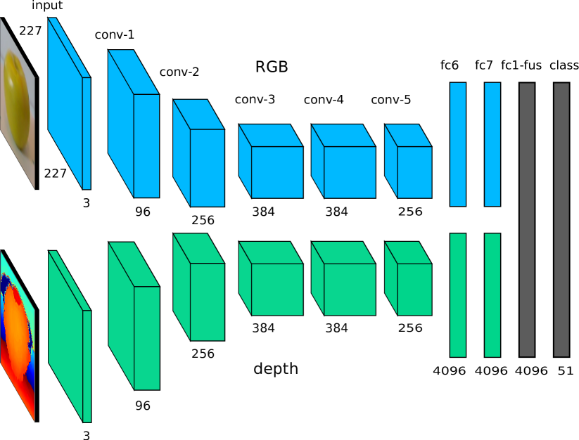
Our approach builds on recent advances from the machine learning and computer vision community. Specifically, we extend classical convolutional neural network networks (CNNs), which have recently been shown to be remarkably successful for recognition on RGB images [13], to the domain of RGB-D data. Our architecture, which is depicted in Fig. 1, consists of two convolutional network streams operating on color and depth information respectively. The network automatically learns to combine these two processing streams in a late fusion approach. This architecture bears similarity to other recent multi-stream approaches [21, 23, 11]. Training of the individual stream networks as well as the combined architecture follows a stage-wise approach. We start by separately training the networks for each modality, followed by a third training stage in which the two streams are jointly fine-tuned, together with a fusion network that performs the final classification. We initialize both the RGB and depth stream network with weights from a network pre-trained on the ImageNet dataset [19]. While initializing an RGB network from a pre-trained ImageNet network is straight-forward, using such a network for processing depth data is not. Ideally, one would want to directly train a network for recognition from depth data without pre-training on a different modality which, however, is infeasible due to lack of large scale labeled depth datasets. Due to this lack of labeled training data, a pre-training phase for the depth-modality – leveraging RGB data – becomes of key importance. We therefore propose a depth data encoding to enable re-use of CNNs trained on ImageNet for recognition from depth data. The intuition – proved experimentally – is to simply encode a depth image as a rendered RGB image, spreading the information contained in the depth data over all three RGB channels and then using a standard (pre-trained) CNN for recongition.
In real-world environments, objects are often subject to occlusions and sensor noise. In this paper, we propose a data augmentation technique for depth data that can be used for robust training. We augment the available training examples by corrupting the depth data with missing data patterns sampled from real-world environments. Using these two techniques, our system can both learn robust depth features and implicitly weight the importance of the two modalities.
We tested our method to support our claims: first, we report on RGB-D recognition accuracy, then on robustness with respect to real-world noise. For the first, we show that our work outperforms the current state of the art on the RGB-D Object dataset of Lai et al. [15]. For the second, we show that our data augmentation approach improves object recognition accuracy in a challenging real-world and noisy environment using the RGB-D Scenes dataset [16].

II Related Work
Our approach is related to a large body of work on both convolutional neural networks (CNNs) for object recognition as well as applications of computer vision techniques to the problem of recognition from RGB-D data. Although a comprehensive review of the literature on CNNs and object recognition is out of the scope of this paper, we will briefly highlight connections and differences between our approach and existing work with a focus on recent literature.
Among the many successful algorithms for RGB-D object recognition a large portion still relies on hand designed features such as SIFT in combination with multiple shape features on the depth channel [15, 14]. However, following their success in many computer vision problems, unsupervised feature learning methods have recently been extended to RGB-D recognition settings. Blum et al. [3] proposed an RGB-D descriptor that relies on a K-Means based feature learning approach. More recently Bo et al. [5] proposed hierarchical matching pursuit (HMP), a hierarchical sparse-coding method that can learn features from multiple channel input. A different approach pursued by Socher et al. [22] relies on combining convolutional filters with a recursive neural network (a specialized form of recurrent neural network) as the recognition architecture. Asif et al. [1] report improved recognition performance using a cascade of Random Forest classifiers that are fused in a hierarchical manner. Finally, in recent independent work Schwarz et al. [20] proposed to use features extracted from CNNs pre-trained on ImageNet for RGB-D object recognition. While they also make use of a two-stream network they do not fine-tune the CNN for RGB-D recognition, but rather just use the pre-trained network as is. Interestingly, they also discovered that simple colorization methods for depth are competitive to more involved preprocessing techniques. In contrast to their work, ours achieves higher accuracy by training our fusion CNN end-to-end: mapping from raw pixels to object classes in a supervised manner (with pre-training on a related recognition task). The features learned in our CNN are therefore by construction discriminative for the task at hand. Using CNNs trained for object recognition has a long history in computer vision and machine learning. While they have been known to yield good results on supervised image classification tasks such as MNIST for a long time [17], recently they were not only shown to outperform classical methods in large scale image classification tasks [13], object detection [9] and semantic segmentation [8] but also to produce features that transfer between tasks [7, 2]. This recent success story has been made possible through optimized implementations for high-performance computing systems, as well as the availability of large amounts of labeled image data through, e.g., the ImageNet dataset [19].
While the majority of work in deep learning has focused on 2D images, recent research has also been directed towards using depth information for improving scene labeling and object detection [6, 10]. Among them, the work most similar to ours is the one on object detection by Gupta et al. [10] who introduces a generalized method of the R-CNN detector [9] that can be applied to depth data. Specifically, they use large CNNs already trained on RGB images to also extract features from depth data, encoding depth information into three channels (HHA encoding). Specifically, they encode for each pixel the height above ground, the horizontal disparity and the pixelwise angle between a surface normal and the gravity direction. Our fusion network architecture shares similarities with their work in the usage of pre-trained networks on RGB images. Our method differs in both the encoding of depth into color image data and in the fusion approach taken to combine information from both modalities. For the encoding step, we propose an encoding method for depth images (’colorizing’ depth) that does not rely on complicated preprocessing and results in improved performance when compared to the HHA encoding. To accomplish sensor fusion we introduce additional layers to our CNN pipeline (see Fig. 1) allowing us to automatically learn a fusion strategy for the recognition task – in contrast to simply training a linear classifier on top of features extracted from both modalities. Multi-stream architectures have also been used for tasks such as action recognition [21], detection [11] and image retrieval [23]. An interesting recent overview of different network architectures for fusing depth and image information is given in Saxena et al. [18]. There, the authors compared different models for multimodal learning: (1) early fusion, in which the input image is concatenated to the existing image RGB channels and processed alongside; (2) an approach we denote as late fusion, where features are trained separately for each modality and then merged at higher layers; (3) combining early and late fusion; concluding that late fusion (2) and the combined approach perform best for the problem of grasp detection. Compared to their work, our model is similar to the late fusion approach but widely differs in training – Saxena et al. [18] use a layer-wise unsupervised training approach – and scale (the size of both their networks and input images is an order of magnitude smaller than in our settings).
III Multimodal architecture for RGB-D object recognition
An overview of the architecture is given in Fig. 1. Our network consists of two streams (top-blue and bottom-green part in the figure) – processing RGB and depth data independently – which are combined in a late fusion approach. Each stream consists of a deep CNN that has been pre-trained for object classification on the ImageNet database (we use the CaffeNet [12] implementation of the CNN from Krizhevsky et al. [13]). The key reason behind starting from a pre-trained network is to enable training a large CNN with millions of parameters using the limited training data available from the Washington RGB-D Object dataset (see, e.g., Yosinski et al. [25] for a recent discussion). We first pre-process data from both modalities to fully leverage the ImageNet pre-training. Then, we train our multimodal CNN in a stage-wise manner. We fine-tune the parameters of each individual stream network for classification of the target data and proceed with the final training stage in which we jointly train the parameters of the fusion network. The different steps will be outlined in the following sections.
III-A Input preprocessing
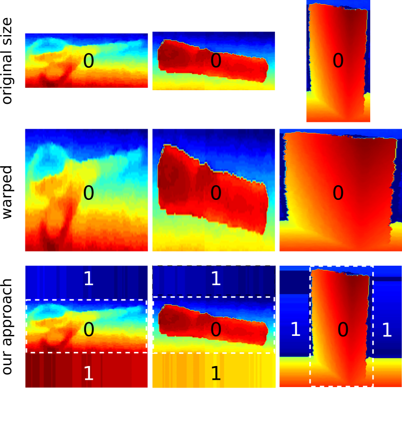
To fully leverage the power of CNNs pre-trained on ImageNet, we pre-process the RGB and depth input data such that it is compatible with the kind of original ImageNet input. Specifically, we use the reference implementation of the CaffeNet [12] that expects 227 227 pixel RGB images as input which are typically randomly cropped from larger 256 256 RGB images (see implementation details on data augmentation). The first processing step consists of scaling the images to the appropriate image size. The simplest approach to achieve this is to use image warping by directly rescaling the original image to the required image dimensions, disregarding the original object ratio. This is depicted in Fig. 3 (middle). We found in our experiments that this process is detrimental to object recognition performance – an effect that we attribute to a loss of shape information (see also Section IV-C). We therefore devise a different preprocessing approach: we scale the longest side of the original image to 256 pixels, resulting in a 256 N or an N 256 sized image. We then tile the borders of the longest side along the axis of the shorter side. The resulting RGB or depth image shows an artificial context around the object borders (see Fig. 3). The same scaling operation is applied to both RGB and depth images.
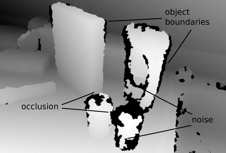
While the RGB images can be directly used as inputs for the CNNs after this processing step, the rescaled depth data requires additional steps. To realize this, recall that a network trained on ImageNet has been trained to recognize objects in images that follow a specific input distribution (that of natural camera images) that is incompatible with data coming from a depth sensor – which essentially encodes distance of objects from the sensor. Nonetheless, by looking at a typical depth image from a household object scene (c.f., Fig. 4) one can conclude that many features that qualitatively appear in RGB images – such as edges, corners, shaded regions – are also visible in, e.g., a grayscale rendering of depth data. This realization has previously led to the idea of simply using a rendered version of the recorded depth data as an input for CNNs trained on ImageNet [10]. We compare different such encoding strategies for rendering depth to images in our experiments. The two most prevalent such encodings are (1) rendering of depth data into grayscale and replicating the grayscale values to the three channels required as network input; (2) using surface normals where each dimension of a normal vector corresponds to one channel in the resulting image. A more involved method, called HHA encoding [10], encodes in the three channels the height above ground, horizontal disparity and the pixelwise angle between a surface normal and the gravity direction.
We propose a fourth, effective and computationally inexpensive, encoding of depth to color images, which we found to outperform the HHA encoding for object recognition. Our method first normalizes all depth values to lie between 0 and 255. Then, we apply a jet colormap on the given image that transforms the input from a single to a three channel image (colorizing the depth). For each pixel in the depth image of size , we map the distance to color values ranging from red (near) over green to blue (far), essentially distributing the depth information over all three RGB channels. Edges in these three channels often correspond to interesting object boundaries. Since the network is designed for RGB images, the colorization procedure provides enough common structure between a depth and an RGB image to learn suitable feature representations (see Fig. 2 for a comparison between different depth preprocessing methods).
III-B Network training
Let be the labeled data available for training our multimodal CNN; with denoting the RGB and pre-processed depth image respectively and corresponding to the image label in one-hot encoding – i.e., is a vector of dimensionality M (the number of labels) with for the position denoting the image label. We train our model using a three-stage approach, first training the two stream networks individually followed by a joint fine-tuning stage.
III-B1 Training the stream networks
We first proceed by training the two individual stream networks (c.f., the blue and green streams in Fig. 1). Let be the representation extracted from the last fully connected layer (fc7) of the CaffeNet – with parameters – when applied to an RGB image . Analogously, let be the representation for the depth image. We will assume that all parameters and (the network weights and biases) are initialized by copying the parameters of a CaffeNet trained on the ImageNet dataset. We can then train an individual stream network by placing a randomly initialized softmax classification layer on top of and and minimizing the negative log likelihood of the training data. That is, for the depth image stream network we solve
| (1) |
where are the weights of the softmax layer mapping from to , the softmax function is given by and the loss is computed as . Training the RGB stream network then can be performed by an analogous optimization. After training, the resulting networks can be used to perform separate classification of each modality.
III-B2 Training the fusion network
Once the two individual stream networks are trained we discard their softmax weights, concatenate their – now fine-tuned – last layer responses and and feed them through an additional fusion stream with parameters . This fusion network again ends in a softmax classification layer. The complete setup is depicted in Fig. 1, where the two fc7 layers (blue and green) are concatenated and merge into the fusion network (here the inner product layer fc1-fus depicted in gray). Analogous to Eq. (1) the fusion network can therefore be trained by jointly optimizing all parameters to minimize the negative log likelihood
| (2) |
where , . Note that in this stage training can also be performed by optimizing only the weights of the fusion network (effectively keeping the weights from the individual stream training intact).
III-C Robust classification from depth images
Finally, we are interested in using our approach in real world robotics scenarios. Robots are supposed to perform object recognition in cluttered scenes where the perceived sensor data is subject to changing external conditions (such as lighting) and sensor noise. Depth sensors are especially affected by a non-negligible amount of noise in such setups. This is mainly due to the fact that reflective properties of materials as well as their coating, often result in missing depth information. An example of noisy depth data is depicted in Fig. 4. In contrast to the relatively clean training data from the Washington RGB-D Object dataset, the depicted scene contains considerable amounts of missing depth values and partial occlusions (the black pixels in the figure). To achieve robustness against such unpredictable factors, we propose a new data augmentation scheme that generates new, noised training examples for training and is tailored specifically to robust classification from depth data.
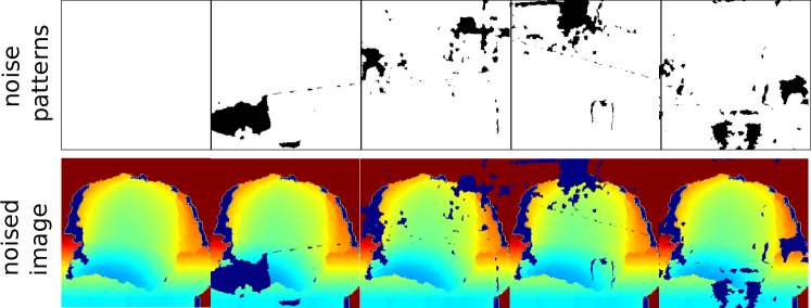
Our approach utilizes the observation that noise in depth data often shows a characteristic pattern and appears at object boundaries or object surfaces. Concretely, we sampled a representative set of noise patterns that occur when recording typical indoor scenes through a Kinect sensor. For sampling the noise patterns we used the RGB-D SLAM dataset [24]. First, we extract 33,000 random noise patches of size 256 256 from different sequences at varying positions and divide them into five groups, based on the number of missing depth readings they contain. Those noise patches are 2D binary masks patterns. We randomly sample pairs of noise patches from two different groups that are randomly added or subtracted and optionally inverted to produce a final noise mask pattern. We repeat this process until we have collected noise patterns in total. Examples of the resulting noise patterns and their application to training examples are shown in Fig. 5.
Training the depth network with artificial noise patterns then proceeds by minimizing the objective from Equation Eq. (1) in which each depth sample is randomly replaced with a noised variant with probability . Formally,
| (3) |
where denotes the Hadamard product, the Bernoulli distribution and the discrete uniform distribution.
IV Experiments
We evaluate our multimodal network architecture on the Washington RGB-D Object Dataset [15] which consists of household objects belonging to 51 different classes. As an additional experiment – to evaluate the robustness of our approach for classification in real-world environments – we considered classification of objects from the RGB-D Scenes dataset whose class distribution partially overlaps with the RGB-D Object Dataset.
IV-A Experimental setup
All experiments were performed using the publicly available Caffe framework [12]. As described previously we use the CaffeNet as the basis for our fusion network. It consists of five convolutional layers (with max-pooling after the first, second and fifth convolution layer) followed by two fully connected layers and a softmax classification layer. Rectified linear units are used in all but the final classification layer. We initialized both stream networks with the weights and biases of the first eight layers from this pre-trained network, discarding the softmax layer. We then proceeded with our stage-wise training. In the first stage (training the RGB and depth streams independently) the parameters of all layers were adapted using a fixed learning rate schedule (with initial learning rate of 0.01 that is reduced to 0.001 after 20K iterations and training is stopped after 30K iterations). In the second stage (training the fusion network, 20k iterations, mini-batch size of 50) we experimented with fine-tuning all weights but found that fixing the individual stream networks (by setting their learning rate to zero) and only training the fusion part of the network resulted in the best performance. The number of training iterations were chosen based on the validation performance on a training validation split in a preliminary experiment. A fixed momentum value of 0.9 and a mini-batch size of 128 was used for all experiments if not stated otherwise. We also adopted the common data augmentation practices of randomly cropping 227 227 sub-images from the larger 256 256 input examples and perform random horizontal flipping. Training of a single network stream takes ten hours, using a NVIDIA 780 graphics card.
IV-B RGB-D Object dataset
| Method | RGB | Depth | RGB-D |
| Nonlinear SVM [15] | 74.5 3.1 | 64.7 2.2 | 83.9 3.5 |
| HKDES [4] | 76.1 2.2 | 75.7 2.6 | 84.1 2.2 |
| Kernel Desc. [14] | 77.7 1.9 | 78.8 2.7 | 86.2 2.1 |
| CKM Desc. [3] | N/A | N/A | 86.4 2.3 |
| CNN-RNN [22] | 80.8 4.2 | 78.9 3.8 | 86.8 3.3 |
| Upgraded HMP [5] | 82.4 3.1 | 81.2 2.3 | 87.5 2.9 |
| CaRFs [1] | N/A | N/A | 88.1 2.4 |
| CNN Features [20] | 83.1 2.0 | N/A | 89.4 1.3 |
| Ours, Fus-CNN (HHA) | 84.1 2.7 | 83.0 2.7 | 91.0 1.9 |
| Ours, Fus-CNN (jet) | 84.1 2.7 | 83.8 2.7 | 91.3 1.4 |
The Washington RGB-D Object Dataset consists of 41,877 RGB-D images containing household objects organized into 51 different classes and a total of 300 instances of these classes which are captured under three different viewpoint angles. For the evaluation every 5th frame is subsampled. We evaluate our method on the challenging category recognition task, using the same ten cross-validation splits as in Lai et al. [15]. Each split consists of roughly 35,000 training images and 7,000 images for testing. From each object class one instance is left out for testing and training is performed on the remaining instances. At test time the task of the CNN is to assign the correct class label to a previously unseen object instance.
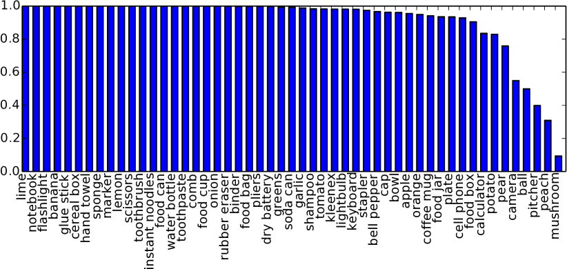
Table I shows the average accuracy of our multi-modal CNN in comparison to the best results reported in the literature. Our best multi-modal CNN, using the jet-colorization, (Fus-CNN jet) yields an overall accuracy of when using RGB and depth ( and when only the RGB or depth modality is used respectively), which – to the best of our knowledge – is the highest accuracy reported for this dataset to date. We also report results for combining the more computationally intensive HHA with our network (Fus-CNN HHA). As can be seen in the table, this did not result in an increased performance. The depth colorization method slightly outperforms the HHA fusion network (Fus-CNN HHA) while being computationally cheaper. Overall our experiments show that a pre-trained CNN can be adapted for recognition from depth data using our depth colorization method. Apart from the results reported in the table, we also experimented with different fusion architectures. Specifically, performance slightly drops to when the intermediate fusion layer (fc1-fus) is removed from the network. Adding additional fusion layers also did not yield an improvement. Finally, Fig. 6 shows the per-class recall, where roughly half of the objects achieve a recall of .
IV-C Depth domain adaptation for RGB-D Scenes
To test the effectiveness of our depth augmentation technique in real world scenes, we performed additional recognition experiments on the more challenging RGB-D Scenes dataset. This dataset consists of six object classes (which overlap with the RGB-D Object Dataset) and a large amount of depth images subjected to noise.
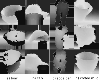
For this experiment we trained two single-stream depth-only networks using the Object dataset and used the Scenes dataset for testing. Further, we assume that the groundtruth bounding box is given in order to report only on recognition performance. The first “baseline” network is trained by following the procedure described in Section III-B1, with the total number of labels . The second network is trained by making use of the depth augmentation outlined in III-C. The results of this experiment are shown in Table II (middle and right column) that reports the recognition accuracy for each object class averaged over all eight video sequences. As is evident from the table, the adapted network (right column) trained with data augmentation outperforms the baseline model for all classes, clearly indicating that additional domain adaptation is necessary for robust recognition in real world scenes. However, some classes (e.g., cap, bowl, soda can) benefit more from noise aware training than others (e.g., flashlight, coffe mug). The kitchen scene depicted in Fig. 4 gives a visual intuition for this result. On the one hand, some objects (e.g., soda cans) often present very noisy object boundaries and surfaces, thus they show improved recognition performance using the adapted approach. On the other hand, small objects (e.g. a flashlight), which are often captured lying on a table, are either less noisy or just small, hence susceptible to be completely erased by the noise from our data augmentation approach. Fig. 7 shows several exemplary noisy depth images from the test set that are correctly classified by the domain-adapted network while the baseline network labels them incorrectly. We also tested the effect of different input image rescaling techniques – previously described in Fig. 3 – in this setting. As shown in the left column of Table II, standard image warping performs poorly, which supports our intuition that shape information gets lost during preprocessing.
| Class | Ours, warp. | Ours, no adapt. | Ours, adapt. |
|---|---|---|---|
| flashlight | 93.4 | 97.5 | 96.4 |
| cap | 62.1 | 68.5 | 77.4 |
| bowl | 57.4 | 66.5 | 69.8 |
| soda can | 64.5 | 66.6 | 71.8 |
| cereal box | 98.3 | 96.2 | 97.6 |
| coffee mug | 61.9 | 79.1 | 79.8 |
| class avg. | 73.6 17.9 | 79.1 14.5 | 82.1 12.0 |
IV-D Comparison of depth encoding methods
Finally, we conducted experiments to compare the different depth encoding methods described in Fig. 2. For rescaling the images, we use our proposed preprocessing method described in Fig. 3 and tested the different depth encoding. Two scenarios are considered: 1) training from scratch using single channel depth images 2) for each encoding method, only fine-tuning the network by using the procedure described in Section III-B1. When training from scratch, the initial learning rate is set to 0.01, then changed to 0.001 after 40K iterations thus stopped after 60K iterations. Training with more iterations did not further improve the accuracy. From the results, presented in Table III, it is clear that training the network from scratch – solely on the RGB-D Dataset – is inferior to fine-tuning. In the latter setting, the results suggest that the simplest encoding method (depth-gray) performs considerably worse than the other three methods. Among these other encodings (which all produce colorized images), surface normals and HHA encoding require additional image preprocessing – meanwhile colorizing depth using our depth-jet encoding has negligible computational overhead. One potential reason why the HHA encoding underperforms in this setup is that all objects are captured on a turntable with the same height above the ground. The height channel used in the HHA encoding therefore does not encode any additional information for solving the classification task. In this experiment, using surface normals yields slightly better performance than the depth-jet encoding. Therefore, we tested the fusion architecture on the ten splits of the RGB-D Object Dataset using the surface normals encoding but this did not further improve the performance. Specifically, the recognition accuracy on the test-set was 91.1 1.6 which is comparable to our reported results in Table I.
V Conclusion
We introduce a novel multimodal neural network archi- tecture for RGB-D object recognition, which achieves state of the art performance on the RGB-D Object dataset [15]. Our method consists of a two-stream convolutional neural network that can learn to fuse information from both RGB and depth automatically before classification. We make use of an effective encoding method from depth to image data that allows us to leverage large CNNs trained for object recognition on the ImageNet dataset. We present a novel depth data augmentation that aims at improving recognition in noisy real-world setups, situations typical of many robotics scenarios. We present extensive experimental results and confirm that our method is accurate and it is able to learn rich features from both domains. We also show robust object recognition in real- world environments and prove that noise-aware training is effective and improves recognition accuracy on the RGB-D Scenes dataset [16].
| Depth Encoding | Accuracy |
|---|---|
| Depth-gray (single channel), from scratch | 80.1 2.6 |
| Depth-gray | 82.0 2.8 |
| Surface normals | 84.7 2.3 |
| HHA | 83.0 2.7 |
| Depth-jet encoding | 83.8 2.7 |
References
- [1] U. Asif, M. Bennamoun, and F. Sohel, “Efficient rgb-d object categorization using cascaded ensembles of randomized decision trees,” in Proc. of the IEEE Int. Conf. on Robotics & Automation (ICRA), 2015.
- [2] H. Azizpour, A. S. Razavian, J. Sullivan, A. Maki, and S. Carlsson, “From generic to specific deep representations for visual recognition,” arXiv preprint arxiv:1406.5774, 2014.
- [3] M. Blum, J. T. Springenberg, J. Wuelfing, and M. Riedmiller, “A learned feature descriptor for object recognition in rgb-d data.” in Proc. of the IEEE Int. Conf. on Robotics & Automation (ICRA), 2012.
- [4] L. Bo, K. Lai, X. Ren, and D. Fox, “Object recognition with hierarchical kernel descriptors,” in IEEE Int. Conf. on Computer Vision and Pattern Recognition (CVPR), 2011.
- [5] L. Bo, X. Ren, and D. Fox, “Unsupervised feature learning for rgb-d based object recognition,” in Proc. of the Int. Symposium on Experimental Robotics (ISER), 2012.
- [6] C. Couprie, C. Farabet, L. Najman, and Y. LeCun, “Indoor semantic segmentation using depth information,” in Int. Conf. on Learning Representations (ICLR), 2013.
- [7] J. Donahue, Y. Jia, O. Vinyals, J. Hoffman, N. Zhang, E. Tzeng, and T. Darrell, “Decaf: A deep convolutional activation feature for generic visual recognition,” arXiv preprint arXiv:1310.1531, 2013.
- [8] C. Farabet, C. Couprie, L. Najman, and Y. LeCun, “Learning hierarchical features for scene labeling,” TPAMI, pp. 1915–1929, 2013.
- [9] R. Girshick, J. Donahue, T. Darrell, and J. Malik, “Rich feature hierarchies for accurate object detection and semantic segmentation,” in IEEE Int. Conf. on Computer Vision and Pattern Recognition (CVPR), 2014.
- [10] S. Gupta, R. Girshick, P. Arbeláez, and J. Malik, “Learning rich features from rgb-d images for object detection and segmentation,” in European Conference on Computer Vision (ECCV), 2014.
- [11] B. Hariharan, P. Arbeláez, R. Girshick, and J. Malik, “Simultaneous detection and segmentation,” in European Conference on Computer Vision (ECCV), 2014.
- [12] Y. Jia, E. Shelhamer, J. Donahue, S. Karayev, J. Long, R. Girshick, S. Guadarrama, and T. Darrell, “Caffe: Convolutional architecture for fast feature embedding,” arXiv preprint arXiv:1408.5093, 2014.
- [13] A. Krizhevsky, I. Sutskever, and G. E. Hinton, “Imagenet classification with deep convolutional neural networks,” in Advances in Neural Information Processing Systems (NIPS), 2012.
- [14] L. Bo, X. Ren and D.Fox, “Depth kernel descriptors for object recognition,” in Proc. of the IEEE/RSJ Int. Conf. on Intelligent Robots and Systems (IROS), 2011.
- [15] K. Lai, L. Bo, X. Ren, and D. Fox, “A large-scale hierarchical multi-view rgb-d object dataset,” in Proc. of the IEEE Int. Conf. on Robotics & Automation (ICRA), 2011.
- [16] K. Lai, L. Bo, X. R. Ren, and D. Fox, “Detection-based object labeling in 3d scenes,” in Proc. of the IEEE Int. Conf. on Robotics & Automation (ICRA), 2012.
- [17] Y. Lecun, L. Bottou, Y. Bengio, and P. Haffner, “Gradient-based learning applied to document recognition,” in Proc. of the IEEE, 1998.
- [18] I. Lenz, H. Lee, and A. Saxena, “Deep learning for detecting robotic grasps,” in Proc. of Robotics: Science and Systems (RSS), 2013.
- [19] O. Russakovsky, J. Deng, H. Su, J. Krause, S. Satheesh, S. Ma, Z. Huang, A. Karpathy, A. Khosla, M. Bernstein, A. C. Berg, and L. Fei-Fei, “ImageNet Large Scale Visual Recognition Challenge,” 2014.
- [20] M. Schwarz, H. Schulz, and S. Behnke, “RGB-D object recognition and pose estimation based on pre-trained convolutional neural network features,” in Proc. of the IEEE Int. Conf. on Robotics & Automation (ICRA), 2015.
- [21] K. Simonyan and A. Zisserman, “Two-stream convolutional networks for action recognition in videos,” in Advances in Neural Information Processing Systems(NIPS), 2014.
- [22] R. Socher, B. Huval, B. Bhat, C. D. Manning, and A. Y. Ng, “Convolutional-recursive deep learning for 3d object classification,” in Advances in Neural Information Processing Systems (NIPS), 2012.
- [23] N. Srivastava and R. R. Salakhutdinov, “Multimodal learning with deep boltzmann machines,” in Advances in Neural Information Processing Systems (NIPS), 2012.
- [24] J. Sturm, N. Engelhard, F. Endres, W. Burgard, and D. Cremers, “A benchmark for the evaluation of rgb-d slam systems,” in Proc. of the IEEE/RSJ Int. Conf. on Intelligent Robots and Systems (IROS), 2012.
- [25] J. Yosinski, J. Clune, Y. Bengio, and H. Lipson, “How transferable are features in deep neural networks?” in Advances in Neural Information Processing Systems (NIPS), 2014.