Bayesian inference for diffusion-driven mixed-effects models

Abstract

Stochastic differential equations (SDEs) provide a natural framework for modelling intrinsic stochasticity inherent in many continuous-time physical processes. When such processes are observed in multiple individuals or experimental units, SDE driven mixed-effects models allow the quantification of both between and within individual variation. Performing Bayesian inference for such models using discrete-time data that may be incomplete and subject to measurement error is a challenging problem and is the focus of this paper. We extend a recently proposed MCMC scheme to include the SDE driven mixed-effects framework. Fundamental to our approach is the development of a novel construct that allows for efficient sampling of conditioned SDEs that may exhibit nonlinear dynamics between observation times. We apply the resulting scheme to synthetic data generated from a simple SDE model of orange tree growth, and real data on aphid numbers recorded under a variety of different treatment regimes. In addition, we provide a systematic comparison of our approach with an inference scheme based on a tractable approximation of the SDE, that is, the linear noise approximation.

Keywords: Stochastic differential equation; mixed-effects; Markov chain Monte Carlo; modified innovation scheme; linear noise approximation.

1 Introduction

Diffusion processes satisfying Itô stochastic differential equations (SDEs) are a class of continuous-time, continuous-valued Markov stochastic processes that can be used to model a wide range of phenomena. Examples include (but are not limited to) epidemics, financial time series, population dynamics (including predator-prey systems) and intra-cellular processes. When repeated measurements on a system of interest are made, differences between individuals or experimental units can be incorporated through random effects. Quantification of both system (intrinsic) variation and variation between units leads to a stochastic differential mixed-effects model (SDMEM).

Unfortunately, analytic intractability of SDEs governing most nonlinear multivariate diffusions can make likelihood-based inference methods problematic. Methods to overcome this difficulty include closed-form expansion of the transition density (Aïït-Sahalia,, 2002, 2008; Stramer et al.,, 2010), exact simulation approaches (Beskos et al.,, 2006; Sermaidis et al.,, 2013) and use of the Euler-Maruyama approximation coupled with data augmentation (Pedersen,, 1995; Elerian et al.,, 2001; Eraker,, 2001; Durham and Gallant,, 2002; Golightly and Wilkinson,, 2008; Stramer and Bognar,, 2011; Kou et al.,, 2012). Difficulty in performing inference for SDEs has resulted in relatively little work on SDMEMs.

Picchini et al., (2010) propose a procedure for obtaining approximate maximum likelihood estimates for SDMEM parameters based on a two step approach; they use a closed-form Hermite expansion (Aïït-Sahalia,, 2002, 2008) to approximate the transition density, before using Gaussian quadrature to numerically integrate the conditional likelihood with respect to the random parameters. As noted by Picchini and Ditlevsen, (2011), the approach is, in practice, limited to a scalar random effect parameter since Gaussian quadrature is computationally inefficient when the dimension of the random effect parameter grows. The methodology is extended in Picchini and Ditlevsen, (2011) to deal with multiple random effects. A number of limitations remain however. In particular a reducible diffusion process is required, that is, one which can be transformed to give a unit diffusion coefficient. Another drawback is that the method cannot account for measurement error. A promising approach appears to be the use of the extended Kalman filter (EKF) to provide a tractable approximation to the SDMEM. This has been the focus of Overgaard et al., (2005), Tornøe et al., (2005) and Berglund et al., (2011). The R package PSM (Klim et al.,, 2009) uses the EKF to estimate SDMEMs. Unfortunately, a quantification of the effect of using these approximate inferential models appears to be missing from the literature. Donnet et al., (2010) discuss inference for SDMEMs in a Bayesian framework, and implement a Gibbs sampler when the SDE (for each experimental unit) has an explicit solution. When no explicit solution exists they suggest that a solution might be found using the Euler-Maruyama discretisation.

1.1 Contributions and organisation of the paper

In this article we provide a method that permits (simulation-based) Bayesian inference for a large class of multivariate SDMEMs using discrete-time observations that may be incomplete (so that only a subset of model components are observed) and subject to measurement error. The method makes use of a novel scheme that allows for observations made sparsely in time, as the process of interest may exhibit nonlinear dynamics between measurement times.

As a starting point, we consider a data augmentation approach that adopts an Euler-Maruyama approximation of unavailable transition densities and augments low frequency data with additional time points over which the approximation is satisfactory. Although a discretisation bias is introduced, this can be made arbitrarily small (at greater computational expense). Moreover, the approach is flexible, and is not restricted to reducible diffusions. A Bayesian approach then aims to construct the joint posterior density for parameters and the components of the latent process. The intractability of the posterior density necessitates simulation techniques such as Markov chain Monte Carlo. As is well documented in Roberts and Stramer, (2001), care must be taken in the design of the MCMC sampler due to dependence between the parameters entering the diffusion coefficient and the latent process. We therefore adapt the reparameterisation technique (known as the modified innovation scheme) of Golightly and Wilkinson, (2008) and Golightly and Wilkinson, (2010) (see also Stramer and Bognar, (2011); Fuchs, (2013); Papaspiliopoulos et al., (2013)) to the SDMEM framework. A key requirement of the scheme is the ability to sample the latent process between two fixed values. Previous approaches have typically focused on the modified diffusion bridge construct of Durham and Gallant, (2002). For the SDMEM considered in Section 5.2 we find that this construct fails to capture the nonlinear dynamics exhibited between observation times. We therefore develop a novel bridge construct that is simple to implement and can capture nonlinear behaviour.

Finally, we provide a systematic comparison of our approach with an inference scheme based on a linear noise approximation (LNA) of the SDE. The LNA approximates transition densities as Gaussian, and when combined with Gaussian measurement error, allows the latent process to be integrated out analytically. Essentially a forward (Kalman) filter can be implemented to calculate the marginal likelihood of all parameters of interest, allowing a marginal Metropolis-Hastings scheme targeting their posterior distribution. It should be noted, however, that evaluation of the Gaussian transition densities under the LNA require the solution of an ordinary differential equation (ODE) system whose order grows quadratically with the number of components (say $d$) governed by the SDE. The computational efficiency of an LNA based inference scheme will therefore depend on $d$, and on whether or not the ODE system can be solved analytically.

We apply the methods to two examples. First, we consider a synthetic dataset generated from an SDMEM driven by the simple univariate model of orange tree growth presented in Picchini et al., (2010) and Picchini and Ditlevsen, (2011). The ODE system governing the LNA solution is tractable in this example. Second, we fit a model of aphid growth to both real and synthetic data. The real data are taken from Matis et al., (2008) and consist of Cotton aphid (Aphis gossypii) counts in the Texas High Plains obtained for three different levels of irrigation water, nitrogen fertiliser and block. This application is particularly challenging, due to the nonlinear drift and diffusion coefficients governing the SDMEM and the ability to only observe one of the model components (with error). Moreover, the ODE system governing the LNA solution is intractable and a numerical solver must be used.

The remainder of the article is organised as follows. The SDMEM framework is introduced in Section 2. Section 3 provides MCMC methods for Bayesian inference, with a novel bridge construct outlined in Section 3.2. The linear noise approximation and its application as an inferential model is discussed in Section 4. The methods are applied in Section 5 before conclusions are drawn in Section 6.

2 Stochastic Differential Mixed-effects models

Consider the case where we have $N$ experimental units randomly chosen from a theoretical population, and associated with each unit $i$ is a continuous-time $d$-dimensional Itô process $\{X_{t}^{i},t\geq 0\}$ governed by the SDE

$$dX_{t}^{i}=\alpha(X_{t}^{i},\theta,b^{i})\,dt+\sqrt{\beta(X_{t}^{i},\theta,b^{i})}\,dW_{t}^{i},\quad X_{0}^{i}=x_{0}^{i},\quad i=1,\ldots,N.$$ (1)

Here, $\alpha$ is a $d$-vector of drift functions, the diffusion coefficient $\beta$ is a $d\times d$ positive definite matrix with a square root representation $\sqrt{\beta}$ such that $\sqrt{\beta}\sqrt{\beta}^{T}=\beta$ and $W_{t}^{i}$ is a $d$-vector of (uncorrelated) standard Brownian motion processes. The $p$-vector parameter $\theta=(\theta_{1},\ldots,\theta_{p})^{T}$ is common to all units whereas the $q$-vectors $b^{i}=(b_{1}^{i},\ldots,b_{q}^{i})^{T}$, $i=~{}1,\ldots,N$, are unit-specific effects, which may be fixed or random. In the most general random effects scenario we let $\pi(b^{i}|\psi)$ denote the joint distribution of $b^{i}$, parameterised by the $r$-vector $\psi=(\psi_{1},\ldots,\psi_{r})^{T}$. The model defined by (1) allows for differences between experimental units through different realisations of the Brownian motion paths $W_{t}^{i}$ and the random effects $b^{i}$, accounting for inherent stochasticity within a unit, and variation between experimental units respectively.

We assume that each experimental unit $\{X_{t}^{i},t\geq 0\}$ cannot be observed exactly, but observations $y^{i}=(y_{t_{0}}^{i},y_{t_{1}}^{i},\ldots,y_{t_{n}}^{i})^{T}$ are available and these are conditionally independent (given the latent process). We link the observations to the latent process via

$$Y_{t}^{i}=F^{T}X_{t}^{i}+\epsilon_{t},\qquad\epsilon_{t}|\Sigma\overset{indep}{\sim}N(0,\Sigma),$$ (2)

where $Y_{t}^{i}$ is a $d_{o}$-vector, $F$ is a constant $d\times d_{o}$ matrix and $\epsilon_{t}$ is a random $d_{o}$-vector. Note that this setup allows for only observing a subset of components ($d_{o}<d$) and this aspect is explored further in Section 5.2.

Together (1) and (2) completely specify the stochastic differential mixed-effects model. However, for most problems of interest the form of the SDE associated with each unit will not permit an analytic solution, precluding straightforward inference for the unknown parameters. We therefore work with the Euler-Maruyama approximation

$$\Delta X_{t}^{i}\equiv X^{i}_{t+\Delta t}-X^{i}_{t}=\alpha(X_{t}^{i},\theta,b^{i})\,\Delta t+\sqrt{\beta(X_{t}^{i},\theta,b^{i})}\,\Delta W_{t}^{i}$$

where $\Delta W_{t}^{i}\sim N(0,I_{d}\Delta t)$ and $\Delta t$ is the length of time between observations, assumed equally spaced for notational simplicity. It is, of course, unlikely that this approximation will be sufficiently accurate over the intervals between observation times and so we adopt a data augmentation scheme. Partitioning [$t_{j},t_{j+1}$] as

$$t_{j}=\tau_{j,0}<\tau_{j,1}<\tau_{j,2}<\ldots<\tau_{j,m-1}<\tau_{j,m}=t_{j+1}$$

introduces $m-1$ intermediate time points with interval widths of length

$$\Delta\tau\equiv\tau_{j,k+1}-\tau_{j,k}=\frac{t_{j+1}-t_{j}}{m}.$$ (3)

The Euler-Maruyama approximation can then be applied over each interval of width $\Delta\tau$, and the associated discretisation bias can be made arbitrarily small at the expense of having to impute $\{X_{t}^{i}\}$ at the intermediate times. We adopt the shorthand notation

$$x_{[t_{j},t_{j+1}]}^{i}\equiv x_{[j,j+1]}^{i}=(x_{\tau_{j,0}}^{i},x_{\tau_{j,1}}^{i},\ldots,x_{\tau_{j,m}}^{i})^{T}$$

for the latent process over the time interval $[t_{j},t_{j+1}]$ for unit $i$. Hence, the complete latent trajectory associated with unit $i$ is given by

$$(x^{i})^{T}=((x_{[0,1]}^{i})^{T},(x_{(1,2]}^{i})^{T}\ldots,(x_{(n-1,n]}^{i})^{T})$$

and we stack all unit-specific trajectories into a matrix $x=(x^{1},\ldots,x^{N})$. Likewise the matrix $y=(y^{1},\ldots,y^{N})$ denotes the entire set of observations. Next we focus on how to perform Bayesian inference for the model quantities $x$, $\theta$, $b=(b^{1},\ldots,b^{N})^{T}$, $\psi$ and $\Sigma$.

3 Bayesian inference

The joint posterior for the common parameters $\theta$, fixed/random effects $b$, hyperparameters $\psi$, measurement error variance $\Sigma$ and latent values $x$ is given by

$$\pi(\theta,\psi,\Sigma,b,x|y)\propto\pi(\theta)\pi(\psi)\pi(\Sigma)\pi(b|\psi)\pi(x|\theta,b)\pi(y|x,\Sigma)$$ (4)

where $\pi(\theta)\pi(\psi)\pi(\Sigma)$ is the joint prior density ascribed to $\theta$, $\psi$ and $\Sigma$. In addition we have that

$$\pi(x|\theta,b)=\prod\limits_{i=1}^{N}\prod\limits_{j=0}^{n-1}\prod\limits_{k=1}^{m}\pi(x^{i}_{\tau_{j,k}}|x^{i}_{\tau_{j,k-1}},\theta,b^{i})$$ (5)

where

$$\pi(x^{i}_{\tau_{j,k}}|x^{i}_{\tau_{j,k-1}},\theta,b^{i})=N\left(x^{i}_{\tau_{j,k}}\,;\,x^{i}_{\tau_{j,k-1}}+\alpha(x^{i}_{\tau_{j,k-1}}\,\theta,b^{i})\Delta\tau,~{}\beta(x^{i}_{\tau_{j,k-1}},\theta,b^{i})\Delta\tau\right)$$

and $N(\cdot\,;\,m,V)$ denotes the multivariate Gaussian density with mean $m$ and variance $V$. Similarly

$$\pi(y|x,\Sigma)=\prod\limits_{i=1}^{N}\prod\limits_{j=0}^{n}\pi(y_{t_{j}}^{i}|x_{t_{j}}^{i},\Sigma)$$

where $\pi(y_{t_{j}}^{i}|x_{t_{j}}^{i},\Sigma)=N(y_{t_{j}}^{i}\,;\,x_{t_{j}}^{i},\Sigma)$. Given the intractability of the joint posterior distribution in (4) we aim to construct a Markov chain Monte Carlo (MCMC) scheme which generates realisations from this posterior. The form of the SDMEM admits a Gibbs sampling strategy with blocking that sequentially takes draws from the full conditionals
1. $\pi(x|\theta,\psi,\Sigma,b,y)=\pi(x|\theta,\Sigma,b,y)$, 3. $\pi(\theta|\psi,\Sigma,b,x,y)=\pi(\theta|b,x)$, 5. $\pi(\psi|\theta,\Sigma,b,x,y)=\pi(\psi|b)$. 2. $\pi(\Sigma|\theta,\psi,b,x,y)=\pi(\Sigma|x,y)$, 4. $\pi(b|\theta,\psi,\Sigma,x,y)=\pi(b|\theta,\psi,x)$, Further blocking strategies that exploit the conditional dependencies between the model parameters and latent trajectories can be used. For example, in step 1 the latent trajectories can be updated separately for each experimental unit. Likewise, the unit-specific random effects can be updated separately. Where necessary, Metropolis-within-Gibbs updates can be used. We note that as written, this scheme will mix intolerably poorly as the degree of augmentation $m$ is increased due to dependence between the latent values $x$ and the parameters entering the diffusion coefficient (namely $\theta$ and $b$). We refer the reader to Roberts and Stramer, (2001) for a detailed discussion of this problem. A simple mechanism for overcoming this issue is to update the parameters and latent trajectories jointly (and this has been considered for SDE models by Stramer and Bognar, (2011) and Golightly and Wilkinson, (2011)). For SDMEMs a joint update of $\theta$, $b$ and $x$ is likely to result in a sampler with low acceptance rates. We therefore wish to preserve the blocking structure described above and instead adapt the reparameterisation of Golightly and Wilkinson, (2008) to our problem. In what follows, we describe in detail each step of the Gibbs sampler.

3.1 Path updates

The full conditional density of the latent paths for all experimental units is given by

$$\pi(x|\theta,\Sigma,b,y) \propto\pi(x|\theta,b)\pi(y|x,\Sigma)=\prod\limits_{i=1}^{N}\pi(x^{i}|\theta,b^{i})\pi(y^{i}|x^{i},\Sigma)$$

which suggests a scheme where unit-specific paths are updated separately. We now focus on an updating scheme for a single path, and drop $i$ from the notation, writing $x$ in place of $x^{i}$ and $x_{[j,j+1]}$ in place of $x_{[j,j+1]}^{i}$. Since the parameters are fixed throughout this updating step, we also drop them from the notation.

Following Golightly and Wilkinson, (2008) we update $x$ in overlapping blocks of size $2m+1$. Consider times $t_{j}$ and $t_{j+2}$ at which the current values of the latent process are $x_{t_{j}}$ and $x_{t_{j+2}}$. The full conditional density of the latent process over the interval $(t_{j},t_{j+2})$ is given by

$$\pi(x_{(j,j+2)}|x_{t_{j}},y_{t_{j+1}},x_{t_{j+2}})\propto\pi(y_{t_{j+1}}|x_{t_{j+1}})\prod\limits_{l=j}^{j+1}\prod\limits_{k=1}^{m}\pi(x_{\tau_{l,k}}|x_{\tau_{l,k-1}}).$$ (6)

Under the nonlinear structure of the diffusion process, this full conditional is intractable and so we use a Metropolis-Hastings step to generate draws from (6). We use an independence sampler with proposal density of the form

$$q(x_{(j,j+2)}|x_{t_{j}},y_{t_{j+1}},x_{t_{j+2}})=q_{1}(x_{(j,j+1]}|x_{t_{j}},y_{t_{j+1}})\,q_{2}(x_{(j+1,j+2)}|x_{t_{j+1}},x_{t_{j+2}}).$$ (7)

Figure 1 gives an illustration of the updating procedure which can be applied over intervals $(t_{j},t_{j+2})$, $j=0,1,\ldots,n-2$, with two additional Metropolis-Hastings steps (such as those described in Golightly and Wilkinson, (2006)) that allow for updating $x$ at times $t_{0}$ and $t_{n}$. Deriving appropriate forms for $q_{1}$ and $q_{2}$ requires the ability to (approximately) generate a discrete-time realisation of a diffusion process between two time points at which the process is either observed exactly or subject to Gaussian noise. The resulting trajectory is typically referred to as a diffusion bridge.

Figure 1: Path update illustration over a block of size $2m+1$.

Several strategies for constructing diffusion bridges have been proposed in the literature. For example, Pedersen, (1995) used the Euler-Maruyama scheme to generate bridges myopically of the end point. Durham and Gallant, (2002) use a linear Gaussian approximation of the distribution of the process conditional on the value at a previous and future time point, giving a construct known as the modified diffusion bridge. Extensions of this construct to the case of partial observation with additive Gaussian noise can be found in Golightly and Wilkinson, (2008). Whilst this construct can, in principle, be applied to arbitrary nonlinear multivariate diffusion processes, the effect of the Gaussian approximation is to guide the bridge towards the observation in a linear way, unless there is large uncertainty in the observation process. This effect is exacerbated in the case of no measurement error, in which case the resulting construct is independent of the drift of the target process. Consequently, use of the modified diffusion bridge as a proposal mechanism (in a Metropolis-Hastings independence sampler) is likely to result in low acceptance rates, unless the drift is of little importance in dictating the dynamics of the target process between observation times. Several attempts to overcome this issue have been proposed in the recent literature.

A time-dependent combination of the Pedersen and modified diffusion bridge approaches was proposed by Lindström, (2012). However, the resulting construct requires a model specific tuning parameter governing the relative weight of each contribution (either Pedersen or modified diffusion bridge). Moreover, the optimal value (in terms of maximising acceptance rate) may vary between observation intervals. Beskos et al., (2013) use Hybrid Monte Carlo (HMC) on pathspace to generate SDE sample paths under various observation regimes. For the applications considered, the authors found reasonable gains in overall efficiency (as measured by minimum effective sample size per CPU time) over an independence sampler with a Brownian bridge proposal. However, we note that HMC also requires careful choice of tuning parameters (namely the number of steps (and their size) in the leapfrog integrator) to maximise efficiency. Schauer et al., (2014) (see also Papaspiliopoulos and Roberts, (2012)) combine the ideas of Delyon and Hu, (2006) and Clark, (1990) to obtain a bridge based on the addition of a guiding term to the drift of the target SDE. The guiding term requires a tractable approximation of the unavailable transition densities governing the target process over the length of the inter-observation interval. Schauer et al., (2014) suggest using the transition densities associated with a class of linear processes, although we note that finding an approximation that is both accurate and computationally efficient may be difficult in practice. Moreover, such an approximation can suffer from computational efficiency due to the fact that it must be obtained at each intermediate time point.

In the next section we describe a novel bridge construct that requires no tuning parameters, is simple to implement (even when only a subset of components are observed with Gaussian noise), computationally efficient and explicitly allows for the effect of the drift governing the target SDE.

3.2 An improved bridge construct

Consider a typical interval $[t_{j},t_{j+1}]$, partitioned into $m$ sub-intervals as in (3), over which we wish to generate a realisation of $\{X_{t},t\in[t_{j},t_{j+1}]\}$ conditional on $x_{t_{j}}\equiv x_{\tau_{j,0}}$ and the noisy measurement $y_{t_{j+1}}\equiv y_{\tau_{j,m}}$. Our approach builds on the modified diffusion bridge of Durham and Gallant, (2002), which we briefly review before describing our extension.

3.2.1 Modified diffusion bridge

Key to constructing the modified diffusion bridge is an approximation of the joint distribution of $X_{\tau_{j,k}}$ and $Y_{t_{j+1}}$ (conditional on $x_{\tau_{j,k-1}}$). Under the Euler-Maruyama approximation $X_{\tau_{j,k}}|X_{\tau_{j,k-1}}$ and $Y_{t_{j+1}}|X_{\tau_{j,k}}$ are Gaussian, with the expressions for the mean and variance of the latter evaluated at $X_{\tau_{j,k-1}}$ to give a linear Gaussian structure. This leads to the approximation

$$\begin{pmatrix}X_{\tau_{j,k}}\\ Y_{t_{j+1}}\end{pmatrix}\bigg{|}x_{\tau_{j,k-1}} \sim N\left\{\begin{pmatrix}x_{\tau_{j,k-1}}+\alpha_{j,k-1}\Delta\tau\\[1.99997pt] F^{T}[x_{\tau_{j,k-1}}+\alpha_{j,k-1}\Delta^{-}]\end{pmatrix},\right.$$

$$\quad\qquad\qquad\qquad\qquad\left.\begin{pmatrix}\beta_{j,k-1}\Delta\tau&\beta_{j,k-1}F\Delta\tau\\ F^{T}\beta_{j,k-1}\Delta\tau&F^{T}\beta_{j,k-1}F\Delta^{-}+\Sigma\end{pmatrix}\right\}$$ (8)

where $\Delta^{-}=t_{j+1}-\tau_{j,k-1}$ and we have used the shorthand notation $\alpha(x_{\tau_{j,k-1}})=\alpha_{j,k-1}$ and $\beta(x_{\tau_{j,k-1}})=\beta_{j,k-1}$. Conditioning further on $y_{t_{j+1}}$ gives a Gaussian approximation of $\pi(x_{\tau_{j,k}}|x_{\tau_{j,k-1}},y_{t_{j+1}})$, denoted $\widehat{\pi}(x_{\tau_{j,k}}|x_{\tau_{j,k-1}},y_{t_{j+1}})$, which can be sampled recursively to give a bridge $x_{\tau_{j,0}},\ldots,x_{\tau_{j,m}}$. In the case of no measurement error and observation of all components (so that $y_{t_{j+1}}=x_{t_{j+1}}$ and $F=I_{d}$, the $d\times d$ identity matrix), we obtain

$$\widehat{\pi}(x_{\tau_{j,k}}|x_{\tau_{j,k-1}},x_{t_{j+1}})=N\left(x_{\tau_{j,k}}\,;\,x_{\tau_{j,k-1}}+\frac{x_{t_{j+1}}-x_{\tau_{j,k-1}}}{t_{j+1}-\tau_{j,k-1}}\Delta\tau\,,\,\frac{t_{j+1}-\tau_{j,k}}{t_{j+1}-\tau_{j,k-1}}\beta_{j,k-1}\Delta\tau\right)$$

which is the form of the modified diffusion bridge first described by Durham and Gallant, (2002). In this case, $\widehat{\pi}(x_{\tau_{j,k}}|x_{\tau_{j,k-1}},y_{t_{j+1}})$ can be seen as a linear approximation of the Brownian bridge SDE

$$dX_{t}=\frac{X_{t_{j+1}}-X_{t}}{t_{j+1}-t}\,dt+\sqrt{\beta(X_{t})}\,dW_{t}.$$ (9)

Use of (9) has been justified by Delyon and Hu, (2006), who show that the distribution of the target process (conditional on $x_{t_{j+1}}$) is absolutely continuous with respect to the distribution of the solution to (9). We may therefore expect that a Metropolis-Hastings scheme that uses a proposal based on a discretisation of (9) will yield a non-zero acceptance rate as $\Delta\tau\to 0$ (for a rigorous treatment of the limiting forms, we refer the reader to Delyon and Hu, (2006), Stramer and Yan, (2007) and to Papaspiliopoulos and Roberts, (2012) for a recent discussion). However, it should also be noted that the linear drift function governing (9) is independent of the the drift function $\alpha(\cdot)$ governing the target process. Consequently, in situations where realisations of the target SDE (with the same initial condition) exhibit strong and similar nonlinearity over the inter-observation time, the modified diffusion bridge is likely to be unsatisfactory.

3.2.2 Residual bridge

To allow explicitly for dynamics based on the drift, we partition $X_{t}$ into two parts, one that accounts for the drift in a deterministic way, and another as a residual stochastic process. The modified diffusion bridge is then applied to the residual stochastic process rather than the target process itself. The partition we require is

$$X_{t}=\eta_{t}+R_{t},$$ (10)

where $\{\eta_{t},t\in[t_{j},t_{j+1}]\}$ is a deterministic process satisfying the ODE

$$\frac{d\eta_{t}}{dt}=\alpha(\eta_{t}),\quad\eta_{t_{j}}=x_{t_{j}},$$ (11)

and $\{R_{t},t\in[t_{j},t_{j+1}]\}$ is a residual stochastic process satisfying

$$dR_{t} \equiv dX_{t}-d\eta_{t}=\{\alpha(X_{t})-\alpha(\eta_{t})\}dt+\sqrt{\beta(X_{t})}\,dW_{t}.$$ (12)

We note that the partition in (10) is used by Fearnhead et al., (2014) (see also Section 4) to derive a tractable approximation to the intractable transition densities governing $X_{t}$, whereas our primary motivation for (10) is the application of the modified diffusion bridge construct to the residual process, thus giving a proposal that is likely to perform well for arbitrarily fine discretisations and explicitly incorporates the drift of the target SDE. Therefore, we aim to derive an approximation $\widehat{\pi}(r_{\tau_{j,k}}|r_{\tau_{j,k-1}},y_{t_{j+1}})$, that can be sampled recursively for $k=1,\ldots,m$ and combined with the deterministic process (through numerical solution of (11)) via (10) to give a bridge $x_{\tau_{j,0}},\ldots,x_{\tau_{j,m}}$. The scheme is illustrated in Figure 2.

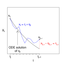
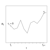
Figure 2: An illustration of the improved bridge construct. Left: The full bridge. Right: A sample path of $R_{t}$.

The initial condition $\eta_{t_{j}}=x_{t_{j}}$ together with the Gaussian measurement error process imply that $r_{t_{j}}=0$ and

$$Y_{t_{j+1}}-F^{T}\eta_{t_{j+1}}=F^{T}R_{t_{j+1}}+\epsilon_{t_{j+1}},\qquad\epsilon_{t_{j+1}}|\Sigma\overset{indep}{\sim}N(0,\Sigma).$$

Hence, it should be clear that the joint distribution of $R_{\tau_{j,k}}$ and $Y_{t_{j+1}}-F^{T}\eta_{t_{j+1}}$ conditional on $R_{\tau_{j,k-1}}=r_{\tau_{j,k-1}}$ can be approximated as

$$\begin{pmatrix}R_{\tau_{j,k}}\\ Y_{t_{j+1}}-F^{T}\eta_{t_{j+1}}\end{pmatrix}\bigg{|}r_{\tau_{j,k-1}} \sim N\left\{\begin{pmatrix}r_{\tau_{j,k-1}}+(\alpha_{j,k-1}-\alpha^{\eta}_{j,k-1})\Delta\tau\\[1.99997pt] F^{T}r_{\tau_{j,k-1}}+F^{T}(\alpha_{j,k-1}-\alpha^{\eta}_{j,k-1})\Delta^{-}\end{pmatrix},\right.$$

$$\quad\qquad\qquad\qquad\left.\begin{pmatrix}\beta_{j,k-1}\Delta\tau&\beta_{j,k-1}F\Delta\tau\\ F^{T}\beta_{j,k-1}\Delta\tau&F^{T}\beta_{j,k-1}F\Delta^{-}+\Sigma\end{pmatrix}\right\}$$

where $\alpha(\eta_{\tau_{j,k-1}})=\alpha^{\eta}_{j,k-1}$. Conditioning further on $y_{t_{j+1}}-F^{T}\eta_{t_{j+1}}$ gives

$$\widehat{\pi}(r_{\tau_{j,k}}|r_{\tau_{j,k-1}},y_{t_{j+1}})=N(r_{\tau_{j,k}};\,\mu_{j,k}\,,\,\Psi_{j,k}),$$ (13)

where

$$\begin{split}\mu_{j,k}&=r_{\tau_{j,k-1}}+(\alpha^{x}_{j,k-1}-\alpha^{\eta}_{j,k-1})\Delta\tau+\beta_{j,k-1}F\Delta\tau(F^{T}\beta_{j,k-1}F\Delta^{-}+\Sigma)^{-1}\\ &\qquad\qquad\qquad\times(y_{t_{j+1}}-F^{T}\eta_{t_{j+1}}-\{F^{T}r_{\tau_{j,k-1}}+F^{T}(\alpha^{x}_{j,k-1}-\alpha^{\eta}_{j,k-1})\Delta^{-}\})\end{split}$$ (14)

and

$$\Psi_{j,k} =\beta_{j,k-1}\Delta\tau-\beta_{j,k-1}F\Delta\tau(F^{T}\beta_{j,k-1}F\Delta^{-}+\Sigma)^{-1}F^{T}\beta_{j,k-1}\Delta\tau.$$ (15)

Together (13)-(15) define our bridge construct. These can be used to define the proposal mechanism in (7) for generating $\{X_{t},t\in[t_{j},t_{j+2}]\}$ by taking

$$q_{1}(x_{(j,j+1]}|x_{t_{j}},y_{t_{j+1}}) =\prod\limits_{k=1}^{m}\widehat{\pi}(x_{\tau_{j,k}}-\eta_{\tau_{j,k}}|r_{\tau_{j,k-1}},y_{t_{j+1}})$$

and

$$q_{2}(x_{(j+1,j+2)}|x_{t_{j+1}},x_{t_{j+2}}) =\prod\limits_{k=1}^{m-1}\widehat{\pi}(x_{\tau_{j+1,k}}-\eta_{\tau_{j+1,k}}|r_{\tau_{j+1,k-1}},x_{t_{j+2}}),$$

where $\widehat{\pi}(x_{\tau_{j+1,k}}-\eta_{\tau_{j+1,k}}|r_{\tau_{j+1,k-1}},x_{t_{j+2}})$ can be sampled using (10) and (13)-(15) with $j$ replaced by $j+1$, $\Sigma=0$ and $F=I_{d}$.

In the special case of no measurement error and observation of all components we have that

$$\widehat{\pi}(r_{\tau_{j,k}}|r_{\tau_{j,k-1}},x_{t_{j+1}})=N\left(r_{\tau_{j,k}}\,;\,r_{\tau_{j,k-1}}+\frac{r_{t_{j+1}}-r_{\tau_{j,k-1}}}{t_{j+1}-\tau_{j,k-1}}\Delta\tau\,,\,\frac{t_{j+1}-\tau_{j,k}}{t_{j+1}-\tau_{j,k-1}}\beta_{j,k-1}\Delta\tau\right),$$

which can be seen as a linear approximation of the Brownian bridge SDE

$$dR_{t}=\frac{R_{t_{j+1}}-R_{t}}{t_{j+1}-t}+\sqrt{\beta(X_{t})}\,dW_{t}.$$ (16)

We also note that (16) has the same diffusion coefficient as the target process and appeal again to Delyon and Hu, (2006), to deduce that the distribution of the residual process governed by (12) (conditional on $r_{t_{j+1}}$) is absolutely continuous with respect to the distribution of the solution to (9).

3.3 Parameter updates

The full conditional densities of $\Sigma$ and $\psi$ are

$$\pi(\Sigma|x,y)\propto\pi(\Sigma)\pi(y|\Sigma)\qquad\text{and}\qquad\pi(\psi|b)\propto\pi(\psi)\pi(b|\psi).$$

Often, semi-conjugate priors can be specified for $\Sigma$ and $\psi$ negating the need for Metropolis-within-Gibbs steps. For the remaining parameters $\theta$ and $b=(b^{1},\ldots,b^{N})^{T}$ we have

$$\pi(\theta|b,x)\propto\pi(\theta)\pi(x|\theta,b)\qquad\text{and}\qquad\pi(b|\theta,\psi,x)\propto\pi(b|\psi)\pi(x|\theta,b)=\prod\limits_{i=1}^{N}\pi(b^{i}|\psi)\pi(x^{i}|\theta,b^{i})$$

where the last expression suggests unit-specific updates of the components of $b$.

As discussed earlier, since $\theta$ and the components of $b$ enter into the diffusion coefficient of (1), sampling the full conditionals of $\theta|b,x$ and $b|\theta,\psi,x$ as part of a Gibbs sampler will result in a reducible Markov chain as $m\to\infty$ (or $\Delta\tau\to 0$). To overcome this problem we use a reparameterisation which is outlined in the next section.

3.3.1 Modified Innovation scheme

The innovation scheme was first outlined in Chib et al., (2004) and exploits the fact that, given $\theta$ and $b$, under the Euler-Maruyama approximation there is a one-to-one relationship between the increments of the process ($\Delta X_{t}$) and the increments of the driving Brownian motion ($\Delta W_{t}$). Moreover, whilst the quadratic variation of $X$ determines $\theta$ and $b$ (as $m\to\infty$), the quadratic variation of the Brownian process is independent of $\theta$ and $b$ a priori. Conditioning on the Brownian increment innovations in a Gibbs update should therefore be effective in overcoming the dependence problem. The resulting algorithm is known as the innovation scheme. Unfortunately, combining an updated parameter value with the Brownian increments will not necessarily give an imputed path that is consistent with the observations. Therefore, Golightly and Wilkinson, (2008, 2010) suggest that a diffusion bridge (such as the modified diffusion bridge of Durham and Gallant, (2002)) be used to determine the innovation process, leading to a modified innovation scheme.

Fuchs, (2013) considers the modified innovation scheme in a continuous-time framework. Adapting their innovation process to an SDMEM, we have, for an interval $[t_{j},t_{j+1}]$, an innovation process $\{Z_{t}^{i},t\in[t_{j},t_{j+1}]\}$ satisfying

$$dZ_{t}^{i} =\beta(X_{t}^{i},\theta,b^{i})^{-{1/2}}\left(dX_{t}^{i}-\frac{x_{t_{j+1}}^{i}-X_{t}^{i}}{t_{j+1}-t}\,dt\right),$$ (17)

$$=\beta(X_{t}^{i},\theta,b^{i})^{-{1/2}}\left\{\alpha(X_{t}^{i},\theta,b^{i})-\frac{x_{t_{j+1}}^{i}-X_{t}^{i}}{t_{j+1}-t}\right\}dt+dW_{t}^{i}$$

with $Z_{t_{j}}^{i}=0$. Clearly, each process $Z^{i}$ has unit diffusion coefficient and whilst not Brownian motion processes, the probability measures induced by each $Z^{i}$ are absolutely continuous with respect to Wiener measure. A proof of this result can be found in Fuchs, (2013) as well as a justification for using this form of innovation process as the effective component in a Gibbs sampler.

The aim is to apply a discretisation of (17) between observation times. We therefore define $x_{o}^{i}=(x_{t_{0}}^{i},\ldots,x_{t_{n}}^{i})^{T}$ to be the current values of the (unit-specific) latent process at the observation times, and stack all $x_{o}^{i}$ values into the matrix $x_{o}$. We have for $k=~{}1,\ldots,m$

$$Z_{\tau_{j,k}}^{i}-Z_{\tau_{j,k-1}}^{i}=\beta^{*}(X_{\tau_{j,k-1}}^{i},\theta,b^{i})^{-{1/2}}\left(X_{\tau_{j,k}}^{i}-X_{\tau_{j,k-1}}^{i}-\frac{x_{t_{j+1}}^{i}-X_{\tau_{j,k-1}}^{i}}{t_{j+1}-\tau_{j,k-1}}\Delta\tau\right),$$

where $Z_{\tau_{j,0}}=0$ and

$$\beta^{*}(X_{\tau_{j,k-1}}^{i},\theta,b^{i})=\frac{t_{j+1}-\tau_{j,k}}{t_{j+1}-\tau_{j,k-1}}\beta(X_{\tau_{j,k-1}}^{i},\theta,b^{i}).$$

Note that our discretisation of (17) follows Golightly and Wilkinson, (2008) by using the modified diffusion bridge to construct the innovation process. Now define a function $f$ so that $X_{\tau_{j,k}}^{i}=f(Z_{\tau_{j,k}}^{i},\theta,b^{i})$ and $Z_{\tau_{j,k}}^{i}=f^{-1}(X_{\tau_{j,k}}^{i},\theta,b^{i})$. Let $z_{imp}^{i}$ denote the (unit-specific) innovation values over $[t_{0},t_{n}]$ and stack all $z_{imp}^{i}$ values into the matrix $z_{imp}$. Define $x_{imp}^{i}$ and $x_{imp}$ similarly. The modified innovation scheme samples $\theta|b,z_{imp},x_{o}$ and $b^{i}|\theta,\psi,z_{imp}^{i},x_{o}^{i}$, $i=1,\ldots,N$. Note that for an updated value of $b^{i}$, say $b^{i*}$, a new $x_{imp}^{i*}$ is updated deterministically through $x_{imp}^{i*}=f(z_{imp}^{i*},\theta,b^{i*})$. Likewise, for a new $\theta^{*}$, a new $x_{imp}^{*}$ is updated deterministically through $x_{imp}^{i*}=f(z_{imp}^{i*},\theta^{*},b^{i})$, $i=1,\ldots,N$. The full conditional density of $\theta$ is

$$\pi(\theta|b,z_{imp},x_{o})\propto\pi(\theta)\prod\limits_{i=1}^{N}\prod\limits_{j=1}^{n-1}\left[\prod\limits_{k=1}^{m}\pi(x^{i}_{\tau_{j,k}}|x^{i}_{\tau_{j,k-1}},\theta,b^{i})\prod\limits_{k=1}^{m-1}J\{f(z_{\tau_{j,k}}^{i},\theta,b^{i})\}\right],$$ (18)

where

$$J\{f(z_{\tau_{j,k}}^{i},\theta,b^{i})\}=\left|\beta^{*}(x^{i}_{\tau_{j,k-1}},\theta,b^{i})\right|^{-{1/2}}$$

is the Jacobian determinant of $f$. Similarly, the full conditional density of $b^{i}$, $i=1,\ldots,N$ is

$$\pi(b^{i}|\theta,\psi,z_{imp}^{i},x_{o}^{i})\propto\pi(b^{i}|\psi)\prod\limits_{j=1}^{n-1}\left[\prod\limits_{k=1}^{m}\pi(x^{i}_{\tau_{j,k}}|x^{i}_{\tau_{j,k-1}},\theta,b^{i})\prod\limits_{k=1}^{m-1}J\{f(z_{\tau_{j,k}}^{i},\theta,b^{i})\}\right].$$ (19)

Naturally, the full conditionals in (18) and (19) will typically be intractable, requiring the use of Metropolis-within-Gibbs updates.

4 Linear noise approximation

In this section we outline a competing solution which uses an inference scheme based on a linear noise approximation (LNA) to the SDMEM. The LNA typically refers to an approximation to the solution of the forward Kolmogorov equation governing the transition probability of a Markov jump process (Kurtz,, 1970; Ferm et al.,, 2008; Komorowski et al.,, 2009; Finkenstädt et al.,, 2013). Specifically, the forward Kolmogorov equation is approximated by a Fokker-Planck equation with linear coefficients. Equivalently, a general Fokker-Planck equation can be deduced and then linearised. In this context, therefore, the LNA aims to replace intractable transition densities with Gaussian approximations. In what follows, we give a brief informal derivation of the LNA and refer the reader to Fearnhead et al., (2014) and the references therein for further details.

4.1 Setup

For notational simplicity and clarity of exposition, we suppress parameter dependence and the unit-specific $i$ for the remainder of this sub-section.

Without loss of generality, consider a time $t\in[t_{j},t_{j+1}]$ at which we wish to approximate the intractable transition density associated with $X_{t}|X_{t_{j}}=x_{t_{j}}$. The LNA uses the same partition of $X_{t}$ given in (10), that is $X_{t}=\eta_{t}+R_{t}$ where the deterministic process $\eta_{t}$ satisfies (11) and the residual stochastic process satisfies (12). The key assumption underpinning the LNA is that the residual stochastic perturbation is “small” relative to the deterministic process, allowing suitable truncation of a Taylor series expansion of $\alpha(X_{t})$ and $\beta(X_{t})$ about $\eta_{t}$. Taking the first two terms in the expansion of $\alpha(X_{t})$, and the first term in the expansion of $\beta(X_{t})$ gives an SDE satisfied by an approximate residual process $\{\tilde{R}_{t},t\in[t_{j},t_{j+1}]\}$ of the form

$$d\tilde{R}_{t}=H_{t}\tilde{R}_{t}\,dt+\sqrt{\beta(\eta_{t})}\,dW_{t},$$ (20)

where $H_{t}$ is the Jacobian matrix with $(i,j)$th element $(H_{t})_{i,j}=\partial\alpha_{i}(\eta_{t})/\partial\eta_{j,t}$.

Assuming fixed or Gaussian initial conditions $\tilde{R}_{t_{j}}\sim N(m_{t_{j}},V_{t_{j}})$ gives $\tilde{R}_{t}\sim N(m_{t},V_{t})$, where $m_{t}$ and $V_{t}$ satisfy the ODE system

$$\dfrac{dm_{t}}{dt} =H_{t}m_{t},$$ (21)

$$\dfrac{dV_{t}}{dt} =H_{t}V_{t}+\beta(\eta_{t},\theta,b)+V_{t}H_{t}^{T}.$$ (22)

In the absence of an analytic solution, the system of coupled ODEs (11) and (21)–(22) which characterise the LNA, must be solved numerically. For initial conditions $\eta_{t_{j}}=~{}x_{t_{j}}$, we have $m_{t_{j}}=0$ and $V_{t_{j}}=0$ so that (21) does not need to be solved, and the approximating transition distribution is $X_{t}|X_{t_{j}}=x_{t_{j}}\sim N(\eta_{t},V_{t})$.

It is worth noting here that the linear form of the SDE (20) satisfied by the approximate residual process coupled with the additive Gaussian observation regime admits a closed form expression for densities of the form $\widehat{\pi}(\tilde{r}_{\tau_{j,k}}|\tilde{r}_{\tau_{j,k-1}},y_{t_{j+1}})$, suggesting use of the LNA as a proposal mechanism inside the Bayesian imputation approach of Section 3. Whilst the LNA could in principle be used to directly approximate the conditioned residual process governed by the SDE in (12) we note that the SDEs in (12) and (20) have different diffusion coefficients. Consequently, the probability law governing $\tilde{R}_{t}$ is not absolutely continuous with respect to the law of $R_{t}$. We therefore do not advocate use of the LNA in this way.

In the next section we outline an inference scheme for SDMEMs of the form (1) based on the LNA. It exploits the computational efficiency of a filtering algorithm proposed by Fearnhead et al., (2014) that allows closed-form calculation of the marginal likelihood $\pi(y|\theta,b,\Sigma)$ under our Gaussian observation regime (2); see the supplementary material for further details.

4.2 Application to SDMEMs

Under the linear noise approximation of (1) the marginal posterior for all parameters is given by

$$\pi(\theta,\psi,\Sigma,b|y) \propto\pi(\theta)\pi(\psi)\pi(\Sigma)\pi(b|\psi)\pi(y|\theta,\Sigma,b)$$

$$\propto\pi(\theta)\pi(\psi)\pi(\Sigma)\prod\limits_{i=1}^{N}\pi(b^{i}|\psi)\pi(y^{i}|\theta,\Sigma,b^{i}).$$

This factorisation suggests a Gibbs sampler with blocking that sequentially takes draws from the full conditionals $\pi(\Sigma|\theta,\psi,b,y)=\pi(\Sigma|y)$, $\pi(\theta|\psi,\Sigma,b,y)=\pi(\theta|b,y)$,$\pi(b|\theta,\psi,\Sigma,y)=\pi(b|\theta,\psi,y)$ and $\pi(\psi|\theta,\Sigma,b,y)=\pi(\psi|b)$. A Metropolis-Hastings step can be used when a full conditional density is intractable. An algorithm for computing the marginal likelihood $\pi(y^{i}|\theta,\Sigma,b^{i})$ for each experimental unit is given in the supplementary material. Interest may also lie in the joint posterior $\pi(\theta,\psi,\Sigma,b,x|y)$ where, since no imputation is required for the LNA, $x^{i}=(x_{t_{0}},\ldots,x_{t_{n}})^{T}$ and $x=(x^{1},\ldots,x^{N})$. Realisations from this posterior can be obtained using the above Gibbs sampler with an extra step that draws from $\pi(x^{i}|\theta,\psi,\Sigma,b^{i},y^{i})=\pi(x^{i}|\theta,\Sigma,b^{i},y^{i})$ for $i=1,\ldots,N$. An efficient mechanism for making such draws can also be found in the supplementary material. The method uses a forward filter, backward sampling (FFBS) algorithm.

5 Applications

We now compare the accuracy and efficiency of our Bayesian imputation approach (coupled with the modified innovation scheme) with an LNA-based solution. We consider two scenarios: one in which the ODEs governing the LNA are tractable and one in which numerical solvers are required. In the first we use synthetic data generated from a simple univariate SDE description of orange tree growth. The second example uses real data taken from Matis et al., (2008) to fit an SDMEM driven by the bivariate diffusion approximation of a stochastic kinetic model of aphid dynamics. The resulting SDMEM is particularly challenging to fit as both the drift and diffusion functions are nonlinear and also only one component of the model is observed (with error). We also include (in the supplementary material) a simulation study based on synthetic data generated from the model of aphid dynamics, to explore further any differences between the Bayesian imputation and LNA-based approaches.

5.1 Orange tree growth

The SDMEM developed by Picchini et al., (2010) and Picchini and Ditlevsen, (2011) to model orange tree growth describes the dynamics of the circumference ($X_{t}^{i}$) of individual trees (mm) by

$$dX_{t}^{i}=\dfrac{1}{\phi_{1}^{i}\phi_{2}^{i}}X_{t}^{i}(\phi_{1}^{i}-X_{t}^{i})\,dt+\sigma\sqrt{X_{t}^{i}}\,dW_{t}^{i},\quad X_{0}^{i}=x_{0}^{i},\quad i=1,\ldots,N$$

with $\phi_{1}^{i}\sim N(\phi_{1},\sigma_{\phi_{1}}^{2})$ and $\phi_{2}^{i}\sim N(\phi_{2},\sigma_{\phi_{2}}^{2})$ independently. Here $\theta=\sigma$ is common to all trees, the random effects are $b^{i}=(\phi_{1}^{i},\phi_{2}^{i})^{T}$, $i=1,\ldots,N$ and the parameter vector governing the random effects distributions is $\psi=(\phi_{1},\phi_{2},\sigma_{\phi_{1}},\sigma_{\phi_{2}})^{T}$. Note that the $\phi_{1}^{i}$ can be interpreted as asymptotic circumferences and the $\phi_{2}^{i}$ as the time-distance between the inflection point of the model obtained by ignoring stochasticity and the point where $X_{t}^{i}=\phi_{1}^{i}/(1+e^{-1})$.

To allow identifiability of all model parameters we generated 16 observations for the circumference of $N=100$ trees at intervals of 100 days. Following Picchini and Ditlevsen, (2011) we gave each tree the same initial condition ($x_{0}^{i}=30$) and took $(\phi_{1},\phi_{2},\sigma_{\phi_{1}},\sigma_{\phi_{2}},\sigma)=(195,350,25,52.5,0.08)$, which gives random effects distributions $\phi_{1}^{i}\sim N(195,25^{2})$ and $\phi_{2}^{i}\sim N(350,52.5^{2})$. For our analysis of these data we assumed the parameters to be independent a priori with $\phi_{1}$ and $\phi_{2}$ having weak $N(0,100^{2})$ priors and $1/\sigma_{\phi_{1}}^{2}$, $1/\sigma_{\phi_{2}}^{2}$ and $1/\sigma^{2}$ having weak gamma $Ga(1,0.01)$ priors. In this example we assume there is no measurement error and therefore the target posterior is given by

$$\pi(\theta,\psi,b|x)\propto\pi(\theta)\pi(\psi)\pi(b|\psi)\pi(x|\theta,b).$$

In the Bayesian imputation approach, $\pi(x|\theta,b)$ is as in (5) whereas for the LNA–based solution

$$\pi(x|\theta,b)=\prod\limits_{i=1}^{N}\prod\limits_{j=0}^{n-1}N(x^{i}_{t_{j+1}}\,;\,\eta^{i}_{t_{j+1}},V^{i}_{t_{j+1}}),$$

where, for each interval $[t_{j},t_{j+1}]$ and each tree $i$, the $\eta_{t}^{i}$ and $V_{t}^{i}$ satisfy the ODE system

$$\dfrac{d\eta_{t}^{i}}{dt} =\dfrac{1}{\phi_{1}^{i}\phi_{2}^{i}}\eta_{t}^{i}(\phi_{1}^{i}-\eta_{t}^{i}),\qquad\eta_{t_{j}}^{i}=x_{t_{j}}^{i},$$

$$\dfrac{dV_{t}^{i}}{dt} =\dfrac{2}{\phi_{1}^{i}\phi_{2}^{i}}(\phi_{1}^{i}-2\eta_{t}^{i})V_{t}^{i}+\sigma^{2}\eta_{t}^{i},\qquad V_{t_{j}}^{i}=0.$$

Fortunately this ODE system can be solved analytically giving $\eta^{i}_{t}=A\phi_{1}^{i}e^{t/\phi_{2}^{i}}/(1+Ae^{t/\phi_{2}^{i}})$ and

$$V_{t}^{i}=B\left(\frac{1}{2}A^{3}\phi_{2}^{i}e^{2t/\phi_{2}^{i}}+3A^{2}\phi_{2}^{i}e^{t/\phi_{2}^{i}}-\phi_{2}^{i}e^{-t/\phi_{2}^{i}}+3At-\dfrac{1}{2}A^{3}\phi_{2}^{i}-3A^{2}\phi_{2}^{i}+\phi_{2}^{i}\right)$$

where $A=x^{i}_{t_{0}}/(\phi_{1}^{i}-x^{i}_{t_{0}})$ and $B=\sigma^{2}A\phi_{1}^{i}e^{2t/\phi_{2}^{i}}/(1+Ae^{t/\phi_{2}^{i}})^{4}$.

The MCMC scheme can make use of simple semi-conjugate updates for $\phi_{1}$, $\phi_{2}$, $\sigma_{\phi_{1}}$ and $\sigma_{\phi_{2}}$. However the remaining parameters ($\sigma$ and the $b^{i}$) require Metropolis-within-Gibbs updates and we have found that componentwise normal random walk updates (so-called random walk Metropolis) on the log scale work particularly well. Also, for the modified innovation scheme, the dynamics of the SDMEM permit the use of the modified diffusion bridge construct to update the latent trajectories between observation times: the improved bridge construct of Section 3.2 is not needed.

The modified innovation scheme requires specification of the level of discretisation $m$. We performed several short pilot runs of the scheme with $m\in\{5,10,20,40\}$ and found no discernible difference in posterior output for $m\geq 10$. We therefore took $m=10$. The sample output was also used to estimate the marginal posterior variances of $\sigma$ and the $b^{i}$, to provide sensible innovation variances in the random walk Metropolis updates. Both the modified innovation scheme and the LNA–based scheme required a burn in of 500 iterations, a thin of 100 iterates and were run long enough to yield a sample of approximately 10K independent posterior draws. Figure 3 shows the marginal posterior densities and autocorrelations for the common parameter $\sigma$ and the parameters governing the random effects distributions. The marginal posterior means and standard deviations of $(\phi_{1},\phi_{2},\sigma_{\phi_{1}},\sigma_{\phi_{2}},\sigma)$ are given in Table 1. The figures and table show that for these parameters both the imputation approach and LNA–based approach generally give similar output and are consistent with the true values from which the data were simulated. Similar results are obtained for the random effects parameters (see the supplementary material).

Both schemes were coded in C and run on an Intel Xeon 3.0GHz processor; the modified innovation scheme took 43504 seconds to run whilst the LNA inference scheme took 2483 seconds. We use the minimum (over each parameter chain) effective sample size (minESS) to measure the statistical efficiency of each scheme. The modified innovation scheme produced a minESS of 7949 and the LNA–based approach gave 7821. Therefore, in terms of minESS/sec, using the LNA outperforms the imputation approach in this example by a factor of approximately 17. It should be noted, however, that for most nonlinear SDMEMs the ODEs governing the LNA solution will rarely be tractable and the consequent use of numerical schemes will degrade its performance.

In the next section we consider an example in which the LNA ODEs are intractable.

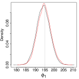
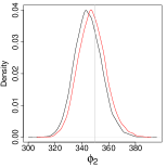
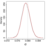
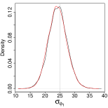
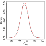
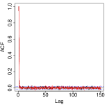
Figure 3: Marginal posterior densities for the random effects hyper-parameters ($\phi_{1}$, $\phi_{2}$, $\sigma_{\phi_{1}}$, $\sigma_{\phi_{2}}$) and common parameter $\sigma$ in the orange tree growth SDMEM, together with their (overlayed) autocorrelation functions. Black: Bayesian imputation. Red: LNA. The vertical grey lines indicate the ground truth.

	$\phi_{1}$	$\phi_{2}$	$\sigma_{\phi_{1}}$	$\sigma_{\phi_{2}}$	$\sigma$
Imputation	194.229	344.799	24.316	53.219	0.079
	(3.509)	(10.098)	(3.149)	(10.410)	(0.002)
LNA	194.634	347.631	24.207	53.960	0.079
	(4.025)	(10.844)	(3.154)	(10.193)	(0.002)

Table 1: Marginal posterior means (standard deviations) of the random effects hyper-parameters ($\phi_{1}$, $\phi_{2}$, $\sigma_{\phi_{1}}$, $\sigma_{\phi_{2}}$) and common parameter $\sigma$ in the orange tree growth SDMEM. The synthetic data used $\phi_{1}=195$, $\phi_{2}=350$, $\sigma_{\phi_{1}}=25$, $\sigma_{\phi_{2}}=52.5$ and $\sigma=0.08$.

5.2 Cotton aphid dynamics

5.2.1 Model and data

Aphids (also known as plant lice or greenfly) are small sap sucking insects which live on the leaves of plants. As they suck the sap they also secrete honey-dew which forms a protective cover over the leaf, ultimately resulting in aphid starvation. Matis et al., (2006) describe a model for aphid dynamics in terms of population size ($N_{t}$) and cumulative population size ($C_{t}$). The model is a stochastic birth-death model with linear birth rate $\lambda N_{t}$ and death rate $\mu N_{t}C_{t}$. The key probabilistic laws governing the time-evolution of the process over a small interval $(t,t+dt]$ are

$$\begin{split}\Pr(N_{t+dt}=n_{t}+1,\,C_{t+dt}=c_{t}+1\,|\,n_{t},c_{t})&=\lambda n_{t}\,dt+o(dt),\\ \Pr(N_{t+dt}=n_{t}-1,\,C_{t+dt}=c_{t}\,|\,n_{t},c_{t})&=\mu n_{t}c_{t}\,dt+o(dt).\end{split}$$ (23)

The diffusion approximation of the Markov jump process defined by (23) is

$$\begin{pmatrix}dN_{t}\\ dC_{t}\\ \end{pmatrix}=\begin{pmatrix}\lambda N_{t}-\mu N_{t}C_{t}\\ \lambda N_{t}\\ \end{pmatrix}dt+\begin{pmatrix}\lambda N_{t}+\mu N_{t}C_{t}&\lambda N_{t}\\ \lambda N_{t}&\lambda N_{t}\\ \end{pmatrix}^{1/2}dW_{t}.$$ (24)

Matis et al., (2008) also provide a dataset of cotton aphid counts collected from three blocks (1/2/3) and using treatments constructed from two factors: water irrigation (low/medium/high) and nitrogen (blanket/variable/none). The data were collected in July 2004 in Lamesa, Texas and consist of five observations of aphid counts aggregated over twenty randomly chosen leaves in each plot for the twenty-seven treatment-block combinations. The data were recorded at times $t=0,1.14,2.29,3.57$ and $4.57$ weeks (approximately every 7/8 days).

We now formulate an appropriate SDMEM model driven by (24) for these data and then fit the model. For notational simplicity, let $i,j,k$ denote the level of water, nitrogen and block number respectively with $i,j,k\in\{1,2,3\}$, where 1 represents low water/blanket nitrogen, 2 represents medium water/variable nitrogen and 3 represents high water/zero nitrogen. Let $N_{t}^{ijk}$ denote the number of aphids at time $t$ for combination $ijk$ and $C_{t}^{ijk}$ the corresponding cumulative population size. We write $X_{t}^{ijk}=(N_{t}^{ijk},C_{t}^{ijk})^{T}$ and consider the SDMEM

$$dX_{t}^{ijk}=\alpha(X_{t}^{ijk},b^{ijk})\,dt+\sqrt{\beta(X_{t}^{ijk},b^{ijk})}\,dW_{t}^{ijk},\quad i,j,k\in\{1,2,3\},$$

where

$$\alpha(X_{t}^{ijk},b^{ijk}) =\begin{pmatrix}\lambda^{ijk}N_{t}^{ijk}-\mu^{ijk}N_{t}^{ijk}C_{t}^{ijk}\\ \lambda^{ijk}N_{t}^{ijk}\\ \end{pmatrix},$$

$$\beta(X_{t}^{ijk},b^{ijk}) =\begin{pmatrix}\lambda^{ijk}N_{t}^{ijk}+\mu^{ijk}N_{t}^{ijk}C_{t}^{ijk}&\lambda^{ijk}N_{t}^{ijk}\\ \lambda^{ijk}N_{t}^{ijk}&\lambda^{ijk}N_{t}^{ijk}\\ \end{pmatrix}.$$

The fixed effects $b^{ijk}=(\lambda^{ijk},\mu^{ijk})^{T}$ have a standard structure which allows for main factor and block effects and single factor-block interactions, with

$$\begin{split}\lambda^{ijk}&=\lambda+\lambda_{W_{i}}+\lambda_{N_{j}}+\lambda_{B_{k}}+\lambda_{WN_{ij}}+\lambda_{WB_{ik}}+\lambda_{NB_{jk}}\\ \mu^{ijk}&=\mu+\mu_{W_{i}}+\mu_{N_{j}}+\mu_{B_{k}}+\mu_{WN_{ij}}+\mu_{WB_{ik}}+\mu_{NB_{jk}}.\end{split}$$ (25)

Also for identifiability we use the corner constraints $\lambda_{W_{1}}=\lambda_{N_{1}}=\lambda_{B_{1}}=0$, $\lambda_{WN_{ij}}=\lambda_{WN_{ij}}(1-\kappa_{ij})$, $\lambda_{WB_{ik}}=\lambda_{WB_{ik}}(1-\kappa_{ik})$ and $\lambda_{NB_{jk}}=\lambda_{NB_{jk}}(1-\kappa_{jk})$, where $\kappa_{rs}=\max(\delta_{1r},\delta_{1s})$ and $\delta_{1\cdot}$ is the Kronecker delta, with equivalent constraints on the death rates. The interpretation of (25) is straightforward. For example, $\lambda^{111}=\lambda$ and $\mu^{111}=\mu$ are the baseline birth and death rates inferred using all $5\times 3^{3}=135$ observations, and correspond to the treatment combination low water, blanket nitrogen and block 1. Likewise, all $5\times 3^{2}=45$ observations taken from block 2 inform the main effects of block 2 ($\lambda_{B_{2}}$ and $\mu_{B_{2}}$) relative to the baseline.

A related approach can be found in Gillespie and Golightly, (2010), where the diffusion approximation is eschewed in favour of a further approximation via moment closure. Our approach further differs from theirs by allowing for measurement error and leads to a much improved predictive fit. The measurement error model is in part motivated by an over-dispersed Poisson error structure which we then approximate by a Gaussian distribution. Specifically, we assume that aphid population size $N_{t}$ is observed with Gaussian error and that the error variance is proportional to the latent aphid numbers, giving

$$Y_{t}^{ijk}|N_{t}^{ijk},\sigma\overset{indep}{\sim}N(N_{t}^{ijk},\sigma^{2}N_{t}^{ijk}),\quad t=0,1.14,2.29,3.57,4.57.$$ (26)

5.2.2 Implementation

Our prior beliefs for $1/\sigma^{2}$ are described by a $Ga(a,a)$ distribution. We found little difference in results for $a\in\{0.01,0.1,1\}$ and so here we report results for $a=1$. The prior for the elements in (25) consists of independent components subject to the birth and death rates for each treatment combination $(\lambda^{ijk},\mu^{ijk})$ being positive. The baseline rates $\lambda$ and $\mu$ must be positive and so, following Gillespie and Golightly, (2010), we assign weak $U(-10,10)$ priors to $\log\lambda$ and $\log\mu$ and also to the remaining parameters. We also take a fairly weak $N(24,90)$ prior for each $N_{t_{0}}^{ijk}$ and use a proposal of the form $N(N_{t_{0}}$,$\sigma^{2}N_{t_{0}})$ for updates. The cumulative population sizes must be at least as large as their equivalent population size. However, we do not expect them to be greatly different a priori. We investigated using a truncated distribution of the form $C_{t_{0}}|N_{t_{0}}\sim N(N_{t_{0}},d_{c}^{2})$, $C_{t_{0}}>N_{t_{0}}$ as the prior and found that this led to little difference in posterior output for $d_{c}\in\{1,10,100\}$. We have, therefore, chosen to fix $C_{t_{0}}^{ijk}=N_{t_{0}}^{ijk}$ in our analysis. Note that the form of the prior for $\sigma$ gives a semi-conjugate update. The remaining parameters in (25) are updated using random walk Metropolis on the pairwise $\lambda,\mu$ component blocks $(\lambda,\mu),(\lambda_{W_{2}},\mu_{W_{2}}),(\lambda_{W_{3}},\mu_{W_{3}}),\ldots,(\lambda_{NB_{33}},\mu_{NB_{33}})$.

The nonlinear form of the observation model (26) can be problematic for the modified innovation scheme. In particular, the proposal mechanism for the path update requires an observation model that is linear in $N_{t}$. Therefore, when proposing from the bridge construct in Section 3.2, we replace $\Sigma$ in (14) and (15) with $\sigma^{2}\eta_{N,t_{j+1}}$, where $\eta_{t_{j+1}}=(\eta_{N,t_{j+1}},\eta_{C,t_{j+1}})^{T}$ is the solution of (11). Since the proposal mechanism is corrected for via the Metropolis-Hastings step, no additional approximations to the target distribution are needed.

In order to obtain a statistically efficient implementation of the modified innovation scheme, we investigate the performance of the modified diffusion bridge construct of Durham and Gallant, (2002) and our improved bridge construct of Section 3.2 in a scenario typical of the real dataset. Using the simulation study of Gillespie and Golightly, (2010), we take $(\lambda,\mu)^{T}=(1.75,0.00095)^{T}$, $x_{0}=(28,28)^{T}$ and recursively apply the Euler-Maruyama approximation to give $x_{3.57}=(829.08,1406.07)^{T}$. We then compare the performance of each bridge construct over the final observation interval $[3.57,4.57]$ by taking $y_{4.57}$ as the median of (26) with $\sigma=1$. Figure 4 shows 95% credible regions of the true conditioned process $N_{t}|x_{3.57},y_{4.57}$ (found via Monte Carlo simulation) with 95% credible regions obtained by repeatedly simulating from the modified diffusion bridge and our improved construct. It is clear that the modified diffusion bridge fails to adequately account for the nonlinear behaviour of the conditioned process. Use of each construct as a proposal mechanism inside a Metropolis-Hastings independence sampler (100K iterations) results in an acceptance rate of around 58% for the improved bridge construct and just 1% for the modified diffusion bridge. It is for these reasons that the modified diffusion bridge is eschewed in favour of our improved bridge construct when applying the Bayesian imputation approach.

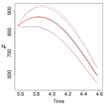
  Improved bridge construct

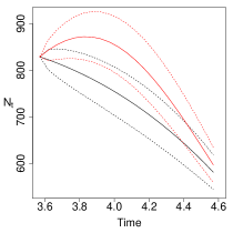
  Modified diffusion bridge

Figure 4: 95% credible region (dashed line) and mean (solid line) of the true conditioned aphid population component $N_{t}|x_{3.57},y_{4.57}$ (red) and two competing bridge constructs (black).

Finally, fitting the LNA requires the solution of an ODE system given by (11) and (22) where the Jacobian matrix is

$$H_{t}=\begin{pmatrix}\lambda-\mu\eta_{C,t}&-\mu\eta_{N,t}\\ \lambda&0\end{pmatrix}.$$

This ODE system is intractable and so our C implementation uses a standard ODE solver from the GNU scientific library, namely the explicit embedded Runge-Kutta-Fehlberg $(4,5)$ method. Note that the tractability of the marginal likelihood under the LNA requires a linear Gaussian observation model. Therefore, when applying the FFBS algorithm in the supplementary material, we make an approximation to the marginal likelihood calculation by replacing $\Sigma$ with $\sigma^{2}\eta_{N,t_{j+1}}$.

5.2.3 Results

The time between observations is almost but not quite constant and so we have allowed each interval to have its own discretisation level, $m$. That said, the interval-specific values vary very little, and by at most two for the larger $m$ values. Several short pilot runs of the modified innovation scheme were performed with typical $m\in\{5,10,20,40,50\}$. These gave no discernible difference in posterior output for $m\geq 20$ and so we took $m=20$. The sample output was also used to estimate the marginal posterior variances of the $\lambda,\mu$ component blocks of the parameters in (25), to be used in the random walk Metropolis updates. Both the modified innovation scheme and MCMC scheme under the LNA were run for 40M iterations with the output thinned by taking every 4Kth iterate to give a final sample of size 10K.

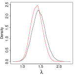
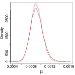
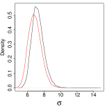
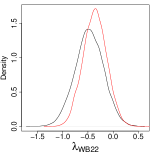
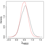
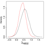
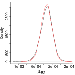
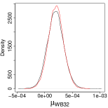
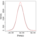
Figure 5: Marginal posterior densities for a selection of the aphid model parameters. Black: Bayesian imputation. Red: LNA.

Figure 5 shows the marginal posterior densities of the baseline parameters, the parameter $\sigma$ controlling the observation error variance and a selection of the remaining parameters. As in Gillespie and Golightly, (2010) we find that block 2 plays an important role. The 95% credible regions for $\mu_{B_{2}}$, the main block 2 death rate, and $\lambda_{NB_{22}}$, the birth rate characterising the interaction with nitrogen, are plausibly non-zero. Whilst the imputation approach and LNA generally give consistent output, there are some notable differences. For example, we find, in general, that the LNA tends to underestimate parameter values (and slightly exaggerates the confidence in these estimates) compared to those obtained under the modified innovation scheme.

We also compared the predictive distributions obtained under each inferential model. The within-sample predictive distribution for the observation process $\{Y_{t},t=0,\ldots,4.57\}$ can be obtained by integrating over the posterior uncertainty of the latent process and parameter values in the observation model (26). Specifically, given samples $\{(n_{t}^{ijk(l)},\sigma^{(l)}),$ $l=1,\ldots,L\}$ from the marginal posterior $\pi(n_{t}^{ijk},\sigma|y)$, the predictive density at time $t$ can be estimated by

$$\frac{1}{L}\sum_{l=1}^{L}N\left(y_{t}\,;\,n_{t}^{ijk(l)},(\sigma^{(l)})^{2}n_{t}^{ijk(l)}\right).$$

Likewise, for a new experiment repeated under the same conditions, the out-of-sample predictive distribution for the aphid population size can be determined for each treatment combination. This is estimated by averaging realisations of $N_{t}$ (obtained by applying the Euler-Maruyama approximation to (24)) over draws from the marginal posterior $\pi(n_{0}^{ijk},b^{ijk}|y)$ obtained using either Bayesian imputation or the LNA. Figures 6 and 7 summarise these predictive distributions for a random selection of treatment combinations. Both the SDMEM and LNA give a satisfactory fit to the observed data, with all observations within or close to the central $50\%$ of the distribution, and no observation outside the equi-tailed $95\%$ credible intervals. As expected, the SDMEM gives a better fit over the LNA, although there is little difference between the two. There are however noticeable differences in the out-of-sample predictives, especially in the lower credible bound (in Figure 7) suggesting that in some situations, using the inferences made under the LNA to predict the outcome of future experiments can give misleading results. These differences lead us to examine the marginal posterior densities of the treatment-block specific birth and death rates, $\lambda^{ijk}$ and $\mu^{ijk}$, over whose uncertainty we average. Samples from these posteriors are straightforward to obtain, using the posterior samples of the constituent parameters in (25). Figure 8 shows marginal posterior densities of the overall birth rates ($\lambda^{ijk}$) associated with the six treatment-block combinations for which predictives are presented in Figure 7. We see distinct differences between posteriors obtained under the Bayesian imputation approach and the LNA approach. The posteriors displayed are indicative of those obtained for all treatment combinations. Moreover, similar patterns are evident in the overall death rates ($\mu^{ijk}$).

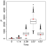
 $ijk=122$

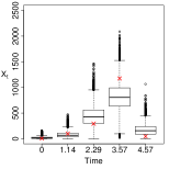
 $ijk=133$

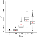
 $ijk=212$

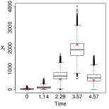
 $ijk=222$

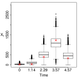
 $ijk=311$

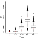
 $ijk=332$

 $ijk=122$

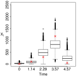
 $ijk=133$

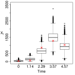
 $ijk=212$

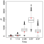
 $ijk=222$

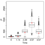
 $ijk=311$

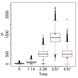
 $ijk=332$

Figure 6: Within sample predictive distributions for Bayesian imputation (top 2 rows) and LNA (bottom 2 rows). The red crosses indicate the observed values.

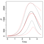
 $ijk=122$

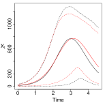
 $ijk=133$

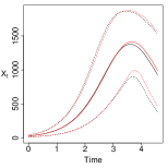
 $ijk=212$

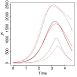
 $ijk=222$

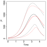
 $ijk=311$

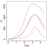
 $ijk=332$

Figure 7: Out-of-sample predictive intervals for the aphid population size $(N_{t}^{ijk})$ against time for a random selection of treatment combinations. The mean is depicted by the solid line with the dashed representing a 95% credible region. Black: Bayesian imputation. Red: LNA.

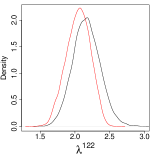
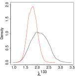
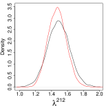
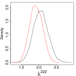
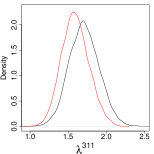
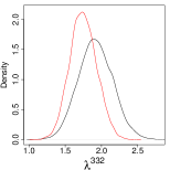
Figure 8: Marginal posterior densities for a random selection of the birth rates associated with specific treatment combinations in the aphid model. Black: Bayesian imputation. Red: LNA.

We obtained a minESS of 1039 under the modified innovation scheme. The LNA, however, clearly benefits from analytically integrating out the latent process and gave a minESS of 8908. For this example, we found that significant gains in computational efficiency were possible by performing the parameter updates and, for the modified innovation scheme, the path updates, in parallel. For example, updating $\lambda_{B_{2}}$ and $\mu_{B_{2}}$ involves calculating a product of likelihoods (or marginal likelihoods for the LNA) over all $3^{2}=9$ treatment combinations that include block 2. These constituent likelihoods can be calculated in parallel. Similarly, for the modified innovation scheme, the treatment specific path updates can be performed in parallel. Both the modified innovation scheme and the LNA–based scheme were again coded in C and run on a high performance computing cluster with 14 cores (made up of Intel Xeon 3.0GHz processors). The modified innovation scheme took approximately 18 days to run whereas the LNA–based scheme required only approximately 4.3 days. Note that here the speed advantage of the LNA–based scheme has reduced, now being roughly 4 times faster than the modified innovation scheme, whereas in Section 5.1, the LNA was approximately 20 times faster. The intractability of the ODEs driving the LNA clearly plays a significant role in computational efficiency. In terms of overall efficiency (as measured by minESS/sec) the LNA–based scheme outperforms the Bayesian imputation approach by a factor of around 36. These computational advantages of the LNA must be weighted against the inaccuracies of the resulting posterior and predictive distributions, inaccuracies which can at times be substantial, as demonstrated by the simulation study in the supplementary material.

6 Discussion

We have provided a framework that permits (simulation-based) Bayesian inference for a large class of multivariate SDMEMs using discrete-time observations that may be incomplete and subject to measurement error. By adopting a Bayesian imputation approach, we have shown how the modified innovation scheme of Golightly and Wilkinson, (2008), which is necessary for overcoming the problematic dependence between the latent process and any parameters that enter the diffusion coefficient, can be applied to SDMEMs. Fundamental to our approach is the development of a novel bridge construct that can be used to sample a discretisation of a conditioned diffusion process, and does not break down when the process exhibits strong nonlinearity over inter-observation times of interest. The computational cost of the Bayesian imputation scheme is dictated by the number of imputed points (characterised by $m$) between observation times. In the examples considered here we see little difference in posterior output under the Bayesian imputation scheme for $m\geq 20$.

We also considered a tractable approximation to the SDMEM, the linear noise approximation, and provided a systematic comparison using two applications. The computational efficiency of the LNA depends on the dimension of the SDE driving the SDMEM. For a $d$-dimensional SDE system, the LNA requires the solution of a system of order $d^{2}$ coupled ODEs. In our first application, the resulting ODE system can be solved analytically, leading to increases in both computational and overall efficiency (as measured by minimum ESS per second) of around a factor of 20. Moreover, we found little difference in the accuracy of inferences made under the LNA and imputation approaches. In our second application, we fitted the diffusion approximation of a Markov jump process description of aphid dynamics using data from Matis et al., (2008). In this example, the ODE system governing the LNA is intractable and the computational advantage of using the LNA over an imputation approach reduced to around a factor of 4. However, the benefit of using the LNA to analytically integrate over the latent process is clear, giving an overall increase in efficiency of around a factor of 36. It is important to note that whilst the LNA is preferred in terms of overall efficiency for the examples considered here, as the dimension $d$ of the SDE is increased, the LNA is likely to become infeasible. Moreover, whilst both the imputation and LNA approaches provided a reasonable fit to the aphid data, differences were found between the parameter posteriors, leading to differences in the out-of-sample predictive distributions. A simulation study (given in the supplementary material) highlighted further differences between the LNA and Bayesian imputation approaches. Care must therefore be taken in trying to fit the SDMEM by using an LNA–based inference approach.

Acknowledgements

The authors would like to thank the associate editor and two anonymous referees for their suggestions which improved the paper.

Supplementary material for Bayesian inference for diffusion-driven mixed-effects models Gavin A. Whitaker¹  Andrew Golightly¹  Richard J. Boys¹  Chris Sherlock^{2 1}School of Mathematics & Statistics, Newcastle University,
Newcastle-upon-Tyne, NE1 7RU, UK
²Department of Mathematics and Statistics, Lancaster University, Lancaster, LA1 4YF

Appendix A LNA FFBS algorithm

To ease the notation, consider a single experimental unit and drop $i$ from the notation. Since the parameters $\theta$, $\psi$, $b$ and $\Sigma$ remain fixed throughout this section, we also drop them from the notation where possible. Define $y_{0:j}=(y_{t_{0}},\ldots,y_{t_{j}})^{T}$. Now suppose that $X_{0}\sim N(a,C)$ a priori. The marginal likelihood under the LNA, $\pi(y|\theta,\Sigma,b)$, can be obtained from the forward filter described below. After execution of the forward filter, realisations of $\pi(x|y,\theta,\Sigma,b)$ can be generated using a backward sampler. Note that the backward sweep requires

$$Cov(X_{t_{j+1}},X_{t_{j}}) =Cov(\tilde{R}_{t_{j+1}},\tilde{R}_{t_{j}})=Cov(P_{t_{j+1}}\tilde{R}_{t_{j}},\tilde{R}_{t_{j}})=P_{t_{j+1}}Var(\tilde{R}_{t_{j}}).$$

Here $P_{t}$ is a $d\times d$ matrix that can be shown to satisfy the ODE

$$\dfrac{dP_{t}}{dt}=H_{t}P_{t},$$ (A.1)

with initial condition $P_{0}=I_{d}$, the $d\times d$ identity matrix.

1. Forward filter. Initialisation. Compute $\pi(y_{t_{0}})=N(y_{t_{0}}\,;\,F^{T}a\,,\,F^{T}CF+\Sigma)$. The posterior at time $t_{0}=0$ is therefore $X_{t_{0}}|y_{t_{0}}\sim N(a_{0},C_{0})$, where

   $$a_{0} =a+CF(F^{T}CF+\Sigma)^{-1}(y_{t_{0}}-F^{T}a)$$

   $$C_{0} =C-CF(F^{T}CF+\Sigma)^{-1}F^{T}C\,.$$

   Store the values of $a_{0}$ and $C_{0}$.

2. For $j=0,1,\ldots,n-1$,

   • Prior at $t_{j+1}$. Initialise the LNA with $\eta_{t_{j}}=a_{t_{j}}$, $V_{t_{j}}=C_{t_{j}}$ and $P_{t_{j}}=I_{d}$. Integrate the ODEs (11), (22) and (A.1) forward to $t_{j+1}$ to obtain $\eta_{t_{j+1}}$, $V_{t_{j+1}}$ and $P_{t_{j+1}}$. Hence $X_{t_{j+1}}|y_{0:j+1}\sim N(\eta_{t_{j+1}},V_{t_{j+1}})$.

   • One step forecast. Using the observation equation, we have that

     $$Y_{t_{j+1}}|y_{0:j}\sim N(F^{T}\eta_{t_{j+1}},F^{T}V_{t_{j+1}}F+\Sigma).$$

     Compute the updated marginal likelihood

     $$\pi(y_{0:j+1}) =\pi(y_{0:j})\pi(y_{t_{j+1}}|y_{0:j})=\pi(y_{0:j})N(y_{t_{j+1}}\,;\,F^{T}\eta_{t_{j+1}}\,,\,F^{T}V_{t_{j+1}}F+\Sigma).$$

   • Posterior at $t_{j+1}$. Combining the distributions in (a) and (b) gives the joint distribution of $X_{t_{j+1}}$ and $Y_{t_{j+1}}$ (conditional on $y_{0:j}$) as

     $$\begin{pmatrix}X_{t_{j+1}}\\ Y_{t_{j+1}}\end{pmatrix}\sim N\left\{\begin{pmatrix}\eta_{t_{j+1}}\\ F^{T}\eta_{t_{j+1}}\end{pmatrix}\,,\,\begin{pmatrix}V_{t_{j+1}}&V_{t_{j+1}}F\\ F^{T}V_{t_{j+1}}&F^{T}V_{t_{j+1}}F+\Sigma\end{pmatrix}\right\}$$

     and therefore $X_{t_{j+1}}|y_{0:j+1}\sim N(a_{t_{j+1}},C_{t_{j+1}})$, where

     $$a_{t_{j+1}} =\eta_{t_{j+1}}+V_{t_{j+1}}F(F^{T}V_{t_{j+1}}F+\Sigma)^{-1}(y_{t_{j+1}}-F^{T}\eta_{t_{j+1}})$$

     $$C_{t_{j+1}} =V_{t_{j+1}}-V_{t_{j+1}}F(F^{T}V_{t_{j+1}}F+\Sigma)^{-1}F^{T}V_{t_{j+1}}\,.$$

     Store the values of $a_{t_{j+1}}$, $C_{t_{j+1}}$, $\eta_{t_{j+1}}$, $V_{t_{j+1}}$ and $P_{t_{j+1}}$.

We sample $\pi(x|y)$ using a backward sampler. The algorithm is as follows.

1. Backward sampler. First draw $x_{t_{n}}$ from $X_{t_{n}}|y\sim N(a_{t_{n}},C_{t_{n}})$.

2. For $j=n-1,n-2,\ldots,0$,

   • Joint distribution of $X_{t_{j}}$ and $X_{t_{j+1}}$. Note that $X_{t_{j}}|y_{0:j}\sim N(a_{t_{j}},C_{t_{j}})$. The joint distribution of $X_{t_{j}}$ and $X_{t_{j+1}}$ (conditional on $y_{0:j}$) is

     $$\begin{pmatrix}X_{t_{j}}\\ X_{t_{j+1}}\end{pmatrix}\sim N\left\{\begin{pmatrix}a_{t_{j}}\\ \eta_{t_{j+1}}\end{pmatrix}\,,\,\begin{pmatrix}C_{t_{j}}&C_{t_{j}}P_{t_{j+1}}^{T}\\ P_{t_{j+1}}C_{t_{j}}&V_{t_{j+1}}\end{pmatrix}\right\}.$$

   • Backward distribution. The distribution of $X_{t_{j}}|X_{t_{j+1}},y_{0:j}$ is $N(\tilde{a}_{t_{j}},\tilde{C}_{t_{j}})$, where

     $$\tilde{a}_{t_{j}} =a_{t_{j}}+C_{t_{j}}P_{t_{j+1}}^{T}V_{t_{j+1}}^{-1}(x_{t_{j+1}}-\eta_{t_{j+1}}),$$

     $$\tilde{C}_{t_{j}} =C_{t_{j}}-C_{t_{j}}P_{t_{j+1}}^{T}V_{t_{j+1}}^{-1}P_{t_{j+1}}C_{t_{j}}.$$

     Draw $x_{t_{j}}$ from $X_{t_{j}}|X_{t_{j+1}},y_{0:j}\sim N(\tilde{a}_{t_{j}},\tilde{C}_{t_{j}})$.

Appendix B Additional graphics from the orange tree growth example

Figure 1 shows the marginal posterior densities of five randomly chosen random effects, based on synthetic data generated from the SDMEM of orange tree growth given in Section 5.1 of the main article.

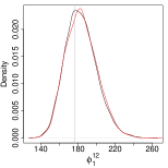
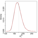
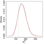
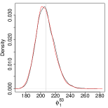
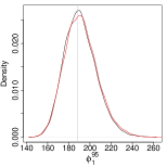
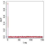
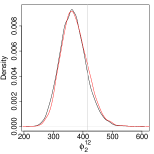
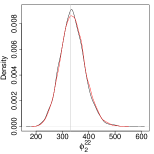
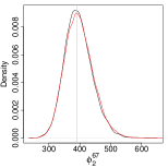
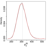
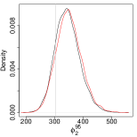
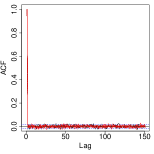
Figure 1: Marginal posterior densities for a random selection of $\phi_{1}^{i}$ (top 2 rows) and $\phi_{2}^{i}$ (bottom 2 rows) in the orange tree growth SDMEM, together with their (overlayed) autocorrelation functions. Black: Bayesian imputation. Red: LNA. The vertical grey lines indicate the ground truth.

Appendix C Simulation study

In this section, we investigate further differences between the Bayesian imputation approach and an inference scheme based on the LNA using synthetic data generated from (24) in the main paper. For simplicity, we consider a fixed treatment (low water, blanket nitrogen) and three blocks. We therefore write $X_{t}^{11k}=(N_{t}^{11k},C_{t}^{11k})^{T}$ and consider the SDMEM

$$dX_{t}^{11k}=\alpha(X_{t}^{11k},b^{11k})\,dt+\sqrt{\beta(X_{t}^{11k},b^{11k})}\,dW_{t}^{11k},\quad k\in\{1,2,3\},$$

where

$$\alpha(X_{t}^{11k},b^{11k}) =\begin{pmatrix}\lambda^{11k}N_{t}^{11k}-\mu^{11k}N_{t}^{11k}C_{t}^{11k}\\ \lambda^{11k}N_{t}^{11k}\\ \end{pmatrix},$$

$$\beta(X_{t}^{11k},b^{11k}) =\begin{pmatrix}\lambda^{11k}N_{t}^{11k}+\mu^{11k}N_{t}^{11k}C_{t}^{11k}&\lambda^{11k}N_{t}^{11k}\\ \lambda^{11k}N_{t}^{11k}&\lambda^{11k}N_{t}^{11k}\\ \end{pmatrix}.$$

The fixed effects $b^{11k}=(\lambda^{11k},\mu^{11k})^{T}$ have a standard structure to incorporate block effects, with

$$\lambda^{11k}=\lambda+\lambda_{B_{k}}\quad\textrm{and}\quad\mu^{11k}=\mu+\mu_{B_{k}},$$

where we again impose the corner constraints $\lambda_{B_{1}}=\mu_{B_{1}}=0$ to allow for identifiability.

To mimic the real dataset, we took $\lambda=1.75$, $\mu=0.00095$, $\lambda_{B2}=-0.1154$, $\lambda_{B3}=-0.0225$, $\mu_{B2}=-0.0004$ and $\mu_{B3}=0.0002$. For each block, we generated five observations (on a regular grid) by using the Euler-Maruyama approximation with a small time-step ($\Delta t=0.001$) and an initial condition of $x_{0}=(5,5)^{T}$. To assess the impact of measurement error on the quality of inferences that can be made about each parameter, we corrupted our data via the observation model

$$Y_{t}^{11k}|N_{t}^{11k},\sigma\overset{indep}{\sim}N(N_{t}^{11k},\sigma^{2}N_{t}^{11k}),\quad t=0,1,2,3,4,$$

and took $\sigma\in\{0,0.5,1,5\}$ to give four synthetic datasets. We adopt the same prior specification for the unknown parameters as used in the real data application.

Both the modified innovation scheme (again incorporating the improved bridge construct) and the LNA-based inference scheme were run long enough to yield a sample of approximately 10K independent posterior draws. For the former, we fixed the discretisation level by taking $m=20$ and note that $m>20$ gave little difference in posterior output. Figure 2 shows the marginal posterior densities of the baseline parameters ($\lambda$ and $\mu$) and the measurement error variance ($\sigma$). The joint posterior densities of $(\mu,\lambda)^{T}$ are shown in Figure 3. It is clear that when fitting the SDMEM using the Bayesian imputation approach, the posterior samples obtained are consistent with the ground truth. This is true to a lesser extent when using the LNA, with the ground truth found in the tail of the posterior distribution in three out of the four scenarios. In fact, when using synthetic data with $\sigma<5$, we see substantive differences in posterior output. As was observed when using real data, the LNA underestimates parameter values compared to those obtained under the Bayesian imputation scheme. In this case, the LNA provides a relatively poor approximation to the true posterior distribution.

Increasing $\sigma$ to 5 (and beyond) gives output from both schemes which is largely in agreement. This is intuitively reasonable, since, as the variance of the measurement process is increased, the ability of both inference schemes to accurately infer the underlying dynamics is diminished. Essentially, the relative difference between the LNA and SDE is reduced.

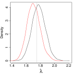
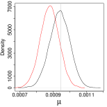
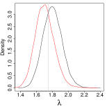
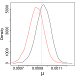
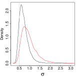
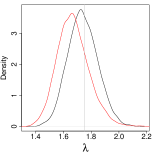
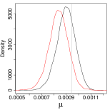
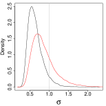
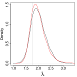
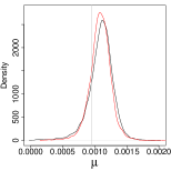
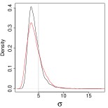
Figure 2: Marginal posterior densities for the baseline parameters and the parameter $\sigma$ controlling the observation error variance in the aphid simulation study. $\sigma=0$ (1${}^{\textrm{st}}$ row), $\sigma=0.5$ (2${}^{\textrm{nd}}$ row), $\sigma=1$ (3${}^{\textrm{rd}}$ row), $\sigma=5$ (4${}^{\textrm{th}}$ row). Black: Bayesian imputation. Red: LNA. The vertical grey lines indicate the ground truth.

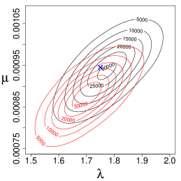
 $\sigma=0$

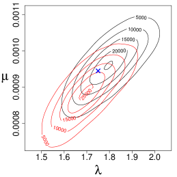
  $\sigma=0.5$

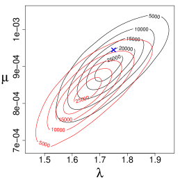
  $\sigma=1$

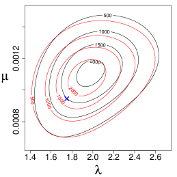
  $\sigma=5$

Figure 3: Bivariate marginal posterior densities for the baseline parameters in the aphid simulation study Black: Bayesian imputation. Red: LNA. The blue cross indicates the ground truth.

References

- Aïït-Sahalia, (2002) Aïït-Sahalia, Y. (2002). Maximum likelihood estimation of discretely sampled diffusions: a closed-form approximation approach. Econometrica, 70(1):223–262.
- Aïït-Sahalia, (2008) Aïït-Sahalia, Y. (2008). Closed-form likelihood expansions for multivariate diffusions. The Annals of Statistics, 36(2):906–937.
- Berglund et al., (2011) Berglund, M., Sunnåker, M., Adiels, M., Jirstrand, M., and Wennberg, B. (2011). Investigations of a compartmental model for leucine kinetics using non-linear mixed effects models with ordinary and stochastic differential equations. Mathematical Medicine and Biology, 29(4):361–384.
- Beskos et al., (2013) Beskos, A., Kalogeropoulos, K., and Pazos, E. (2013). Advanced MCMC methods for sampling on diffusion pathspace. Stochastic Processes and their Applications, 123(4):1415–1453.
- Beskos et al., (2006) Beskos, A., Papaspiliopoulos, O., Roberts, G. O., and Fearnhead, P. (2006). Exact and computationally efficient likelihood-based estimation for discretely observed diffusion processes (with discussion). Journal of the Royal Statistical Society: Series B (Statistical Methodology), 68:333–382.
- Chib et al., (2004) Chib, S., Pitt, M. K., and Shephard, N. (2004). Likelihood based inference for diffusion driven models.
- Clark, (1990) Clark, J. (1990). The simulation of pinned diffusions. In Decision and Control, 1990, Proceedings of the 29th IEEE Conference on, pages 1418–1420. IEEE.
- Delyon and Hu, (2006) Delyon, B. and Hu, Y. (2006). Simulation of conditioned diffusion and application to parameter estimation. Stochastic Processes and their Applications, 116:1660–1675.
- Donnet et al., (2010) Donnet, S., Foulley, J., and Samson, A. (2010). Bayesian analysis of growth curves using mixed models defined by stochastic differential equations. Biometrics, 66(3):733–741.
- Durham and Gallant, (2002) Durham, G. B. and Gallant, A. R. (2002). Numerical techniques for maximum likelihood estimation of continuous-time diffusion processes. Journal of Business and Economic Statistics, 20:297–338.
- Elerian et al., (2001) Elerian, O., Chib, S., and Shephard, N. (2001). Likelihood inference for discretely observed nonlinear diffusions. Econometrica, 69:959–993.
- Eraker, (2001) Eraker, B. (2001). MCMC analysis of diffusion models with application to finance. Journal of Business and Economic Statistics, 19(2):177–191.
- Fearnhead et al., (2014) Fearnhead, P., Giagos, V., and Sherlock, C. (2014). Inference for reaction networks using the linear noise approximation. Biometrics, 70(2):457–466.
- Ferm et al., (2008) Ferm, L., Lötstedt, P., and Hellander, A. (2008). A hierarchy of approximations of the master equation scaled by a size parameter. Journal of Scientific Computing, 34(2):127–151.
- Finkenstädt et al., (2013) Finkenstädt, B., Woodcock, D., Komorowski, M., Harper, C., Davis, J., White, M., and Rand, D. A. (2013). Quantifying intrinsic and extrinsic noise in gene transcription using the linear noise approximation: an application to single cell data. Annals of Applied Statistics, 7:1960–1982.
- Fuchs, (2013) Fuchs, C. (2013). Inference for diffusion processes with applications in Life Sciences. Springer, Heidelberg.
- Gillespie and Golightly, (2010) Gillespie, C. S. and Golightly, A. (2010). Bayesian inference for generalized stochastic population growth models with application to aphids. Journal of the Royal Statistical Society - Series C (Applied Statistics), 59(2):341–357.
- Golightly and Wilkinson, (2006) Golightly, A. and Wilkinson, D. J. (2006). Bayesian sequential inference for nonlinear multivariate diffusions. Statistics and Computing, 16:323–338.
- Golightly and Wilkinson, (2008) Golightly, A. and Wilkinson, D. J. (2008). Bayesian inference for nonlinear multivariate diffusion models observed with error. Computational Statistics & Data Analysis, 52(3):1674–1693.
- Golightly and Wilkinson, (2010) Golightly, A. and Wilkinson, D. J. (2010). Markov chain Monte Carlo algorithms for sde parameter estimation. In Lawrence, N. D., Girolami, M., Rattray, M., and Sanguinetti, G., editors, Learning and inference in Computational Systems Biology, Computational Molecular Biology. MIT Press.
- Golightly and Wilkinson, (2011) Golightly, A. and Wilkinson, D. J. (2011). Bayesian parameter inference for stochastic biochemical network models using particle Markov chain Monte Carlo. Interface Focus, 1(6):807–820.
- Klim et al., (2009) Klim, S., Mortensen, S. B., Kristensen, N. R., Overgaard, R. V., and Madsen, H. (2009). Population stochastic modelling (PSM)-an R package for mixed-effects models based on stochastic differential equations. Computer Methods and Programs in Biomedicine, 94(3):279–289.
- Komorowski et al., (2009) Komorowski, M., Finkenstädt, B., Harper, C., and Rand, D. (2009). Bayesian inference of biochemical kinetic parameters using the linear noise approximation. BMC Bioinformatics, 10(1):343.
- Kou et al., (2012) Kou, S. C., Olding, B. P., Lysy, M., and Liu, J. S. (2012). A multiresolution method for parameter estimation of diffusion processes. Journal of the American Statistical Association, 107:1558–1574.
- Kurtz, (1970) Kurtz, T. G. (1970). Solutions of ordinary differential equations as limits of pure jump markov processes. Journal of Applied Probability, 7(1):49–58.
- Lindström, (2012) Lindström, E. (2012). A regularized bridge sampler for sparsely sampled diffusions. Statistics and Computing, 22(1):615–623.
- Matis et al., (2006) Matis, J. H., Kiffe, T. R., Matis, T. I., and Stevenson, D. E. (2006). Application of population growth models based on cumulative size to Pecan aphids. Journal of Agricultural, Biological, and Environmental Statistics, 11:425–449.
- Matis et al., (2008) Matis, T. I., Parajulee, M. N., Matis, J. H., and Shrestha, R. B. (2008). A mechanistic model based analysis of cotton aphid population dynamics data. Agricultural and Forest Entomology, 10(4):355–362.
- Overgaard et al., (2005) Overgaard, R. V., Jonsson, N., Tornøe, C. W., and Madsen, H. (2005). Non-linear mixed-effects models with stochastic differential equations: implementation of an estimation algorithm. Journal of Pharmacokinetics and Pharmacodynamics, 32(1):85–107.
- Papaspiliopoulos and Roberts, (2012) Papaspiliopoulos, O. and Roberts, G. O. (2012). Importance sampling techniques for estimation of diffusion models. In Statistical Methods for Stochastic Differential Equations , Monographs on Statistics and Applied Probability, pages 311–337. Chapman and Hall.
- Papaspiliopoulos et al., (2013) Papaspiliopoulos, O., Roberts, G. O., and Stramer, O. (2013). Data augmentation for diffusions. Journal of Computational and Graphical Statistics, 22:665–688.
- Pedersen, (1995) Pedersen, A. R. (1995). A new approach to maximum likelihood estimation for stochastic differential equations based on discrete observations. Scandinavian Journal of Statistics, 22(1):55–71.
- Picchini and Ditlevsen, (2011) Picchini, U. and Ditlevsen, S. (2011). Practical estimation of high dimensional stochastic differential mixed-effects models. Computational Statistics and Data Analysis, 55(3):1426–1444.
- Picchini et al., (2010) Picchini, U., Gaetano, S., and Ditlevsen, S. (2010). Stochastic differential mixed-effects models. Scandinavian Journal of Statistics, 37:67–90.
- Roberts and Stramer, (2001) Roberts, G. O. and Stramer, O. (2001). On inference for partially observed nonlinear diffusion models using the Metropolis-Hastings algorithm. Biometrika, 88(3):603–621.
- Schauer et al., (2014) Schauer, M., van der Meulen, F., and van Zanten, H. (2014). Guided proposals for simulating multi-dimensional diffusion bridges. Available from http://arxiv.org/abs/1311.3606.
- Sermaidis et al., (2013) Sermaidis, G., Papaspiliopoulos, O., Roberts, G. O., Beskos, A., and Fearnhead, P. (2013). Markov chain Monte Carlo for exact inference for diffusions. Scandinavian Journal of Statistics, 40:294–321.
- Stramer and Bognar, (2011) Stramer, O. and Bognar, M. (2011). Bayesian inference for irreducible diffusion processes using the pseudo-marginal approach. Bayesian Analysis, 6(2):231–258.
- Stramer et al., (2010) Stramer, O., Bognar, M., and Scheider, P. (2010). Bayesian inference for discretely sampled markov processes with closed-form likelihood expansions. Journal of Financial Econometrics, 8:450–480.
- Stramer and Yan, (2007) Stramer, O. and Yan, J. (2007). Asymptotics of an efficient Monte Carlo estimation for the transition density of diffusion processes. Methodology and Computing in Applied Probability, 9(4):483–496.
- Tornøe et al., (2005) Tornøe, C. W., Overgaard, R. V., Agerso, H., Nielsen, H. A., Madsen, H., and Jonsson, E. N. (2005). Stochastic differential equations in NONMEM: implementation, application, and comparison with ordinary differential equations. Pharmaceutical Research, 22(8):1247–1258.