A Neighbourhood-Based Stopping Criterion for Contrastive Divergence Learning

Abstract

Restricted Boltzmann Machines (RBMs) are general unsupervised learning devices to ascertain generative models of data distributions. RBMs are often trained using the Contrastive Divergence learning algorithm (CD), an approximation to the gradient of the data log-likelihood. A simple reconstruction error is often used as a stopping criterion for CD, although several authors [1, 2] have raised doubts concerning the feasibility of this procedure. In many cases the evolution curve of the reconstruction error is monotonic while the log-likelihood is not, thus indicating that the former is not a good estimator of the optimal stopping point for learning. However, not many alternatives to the reconstruction error have been discussed in the literature. In this manuscript we investigate simple alternatives to the reconstruction error, based on the inclusion of information contained in neighboring states to the training set, as a stopping criterion for CD learning.

I Introduction

Learning algorithms for deep multilayer neural networks have been known for a long time [3], though they usually could not outperform simpler, shallow networks. In this way, deep multilayer networks were not widely used to solve large scale real-world problems until the last decade [4]. In 2006, Deep Belief Networks (DBNs) [5] came out as a real breakthrough in this field, since the learning algorithms proposed ended up being a feasible and practical method to train deep networks, with spectacular results [6, 7, 8, 9]. DBNs have Restricted Boltzmann Machines (RBMs) [10] as their building blocks.

RBMs are topologically constrained Boltzmann Machines (BMs) with two layers, one of hidden and another of visible neurons, and no intralayer connections. This property makes working with RBMs simpler than with regular BMs, and in particular the stochastic computation of the log-likelihood gradient may be performed more efficiently by means of Gibbs sampling [11, 4].

In 2002, the Contrastive Divergence (CD) learning algorithm was proposed as an efficient training method for product-of-expert models, from which RBMs are a special case [12]. It was observed that using CD to train RBMs worked quite well in practice. This fact was important for deep learning since some authors suggested that a multilayer deep neural network is better trained when each layer is pre-trained separately as if it were a single RBM [6, 13, 7]. Thus, training RBMs with CD and stacking up them seems to be a good way to go when designing deep learning architectures.

However, the picture is not as nice as it looks, since CD is not a flawless training algorithm. Despite CD being an approximation of the true log-likelihood gradient [14], it is biased and it may not converge in some cases [15, 16, 17]. Moreover, it has been observed that CD, and variants such as Persistent CD [18] or Fast Persistent CD [19] can lead to a steady decrease of the log-likelihood during learning [2, 20]. Therefore, the risk of learning divergence imposes the requirement of a stopping criterion. There are two main methods used to decide when to stop the learning process. One is based on the monitorization of the reconstruction error [21]. The other is based on the estimation of the log-likelihood with Annealed Importance Sampling (AIS) [22, 23]. The reconstruction error is easy to compute and it has been often used in practice, though its adequacy remains unclear because of monotonicity [2]. AIS seems to work better than the reconstruction error in most cases, though it is considerably more expensive to compute, and may also fail [1].

In this work we approach this problem from a completely different perspective. Based on the fact that the energy is a continuous and smooth function of its variables, the close neighborhood of the high-probability states is expected to acquire also a significant amount of probability. In this sense, we argue that the information contained in the neighborhood of the training data is valuable, and that it can be incorporated in the learning process of RBMs. In particular, we propose to use it in the monitorization of the log-likelihood of the model by means of a new quantity that depends on the information contained in the training set and its neighbors. Furthermore, and in order to make it computationally tractable, we build it in such a way that it becomes independent of the partition function of the model. In this way, we propose a neighborhood-based stopping criterion for CD and show its performance in several data sets.

II Learning in Restricted Boltzmann Machines

II-A Energy-based Probabilistic Models

Energy-based probabilistic models define a probability distribution from an energy function, as follows:

$$P(\mbox{\boldmath$\displaystyle x$},\mbox{\boldmath$\displaystyle h$})=\frac{\displaystyle{e}^{-\text{Energy}(\mbox{\boldmath$\displaystyle x$},\mbox{\boldmath$\displaystyle h$})}}{Z}\ ,$$ (1)

where $\displaystyle x$ and $\displaystyle h$ stand for (typically binary) visible and hidden variables, respectively. The normalization factor $Z$ is called partition function and reads

$$Z=\sum_{\mbox{\boldmath$\displaystyle x$},\mbox{\boldmath$\displaystyle h$}}\displaystyle{e}^{-\text{Energy}(\mbox{\boldmath$\displaystyle x$},\mbox{\boldmath$\displaystyle h$})}\ .$$ (2)

Since only $\displaystyle x$ is observed, one is interested in the marginal distribution

$$P(\mbox{\boldmath$\displaystyle x$})=\frac{\sum_{\mbox{\boldmath$\displaystyle h$}}\displaystyle{e}^{-\text{Energy}(\mbox{\boldmath$\displaystyle x$},\mbox{\boldmath$\displaystyle h$})}}{Z}\ ,$$ (3)

but the evaluation of the partition function $Z$ is computationally prohibitive since it involves an exponentially large number of terms. In this way, one can not measure directly $P(\mbox{\boldmath$\displaystyle x$})$.

The energy function depends on several parameters $\theta$, that are adjusted at the learning stage. This is done by maximizing the likelihood of the data. In energy-based models, the derivative of the log-likelihood can be expressed as

$$-\frac{\partial\log P(\mbox{\boldmath$\displaystyle x$};\theta)}{\partial\theta}=\ E_{P(\mbox{\boldmath$\displaystyle h$}|\mbox{\boldmath$\displaystyle x$})}\left[\frac{\partial\text{Energy}(\mbox{\boldmath$\displaystyle x$},\mbox{\boldmath$\displaystyle h$})}{\partial\theta}\right]$$ (4)

$$\ \ \ \ \ \ \ \ -\ E_{P(\stackrel{{\scriptstyle\thicksim}}{{\mbox{\boldmath$\displaystyle x$}}})}\left[E_{P(\mbox{\boldmath$\displaystyle h$}|\stackrel{{\scriptstyle\thicksim}}{{\mbox{\boldmath$\displaystyle x$}}})}\left[\frac{\partial\text{Energy}(\stackrel{{\scriptstyle\thicksim}}{{\mbox{\boldmath$\displaystyle x$}}},\mbox{\boldmath$\displaystyle h$})}{\partial\theta}\right]\right]\ ,$$

where the first term is called the positive phase and the second term the negative phase. Similar to (3), the exact computation of the derivative of the log-likelihood is usually unfeasible because of the negative phase in (4), which comes from the derivative of the partition function.

II-B Restricted Boltzmann Machines

Restricted Boltzmann Machines are energy-based probabilistic models whose energy function is:

$$\text{Energy}(\mbox{\boldmath$\displaystyle x$},\mbox{\boldmath$\displaystyle h$})=-\mbox{\boldmath$\displaystyle b$}^{t}\mbox{\boldmath$\displaystyle x$}-\mbox{\boldmath$\displaystyle c$}^{t}\mbox{\boldmath$\displaystyle h$}-\mbox{\boldmath$\displaystyle h$}^{t}\mbox{\boldmath$\displaystyle W$}\mbox{\boldmath$\displaystyle x$}\ .$$ (5)

RBMs are at the core of DBNs [5] and other deep architectures that use RBMs for unsupervised pre-training previous to the supervised step [6, 13, 7].

The consequence of the particular form of the energy function is that in RBMs both $P(\mbox{\boldmath$\displaystyle h$}|\mbox{\boldmath$\displaystyle x$})$ and $P(\mbox{\boldmath$\displaystyle x$}|\mbox{\boldmath$\displaystyle h$})$ factorize. In this way it is possible to compute $P(\mbox{\boldmath$\displaystyle h$}|\mbox{\boldmath$\displaystyle x$})$ and $P(\mbox{\boldmath$\displaystyle x$}|\mbox{\boldmath$\displaystyle h$})$ in one step, making it possible to perform Gibbs sampling efficiently, in contrast to more general models like Boltzmann Machines [24].

II-C Contrastive Divergence

The most common learning algorithm for RBMs uses an algorithm to estimate the derivative of the log-likelihood of a Product of Experts model. This algorithm is called Contrastive Divergence [12].

Contrastive Divergence CD_n estimates the derivative of the log-likelihood for a given point $\displaystyle x$ as

$$-\frac{\partial\log P(\mbox{\boldmath$\displaystyle x$};\theta)}{\partial\theta}\simeq\ E_{P(\mbox{\boldmath$\displaystyle h$}|\mbox{\boldmath$\displaystyle x$})}\left[\frac{\partial\text{Energy}(\mbox{\boldmath$\displaystyle x$},\mbox{\boldmath$\displaystyle h$})}{\partial\theta}\right]$$ (6)

$$\ \ \ \ \ \ \ \ -\ E_{P(\mbox{\boldmath$\displaystyle h$}|\mbox{\boldmath$\displaystyle x$}_{n})}\left[\frac{\partial\text{Energy}(\mbox{\boldmath$\displaystyle x$}_{n},\mbox{\boldmath$\displaystyle h$})}{\partial\theta}\right]\ .$$

where $\mbox{\boldmath$\displaystyle x$}_{n}$ is the last sample from the Gibbs chain starting from $\displaystyle x$ obtained after $n$ steps:

• $\mbox{\boldmath$\displaystyle h$}_{1}\sim P(\mbox{\boldmath$\displaystyle h$}|\mbox{\boldmath$\displaystyle x$})$

• $\mbox{\boldmath$\displaystyle x$}_{1}\sim P(\mbox{\boldmath$\displaystyle x$}|\mbox{\boldmath$\displaystyle h$}_{1})$

• …

• $\mbox{\boldmath$\displaystyle h$}_{n}\sim P(\mbox{\boldmath$\displaystyle h$}|\mbox{\boldmath$\displaystyle x$}_{n-1})$

• $\mbox{\boldmath$\displaystyle x$}_{n}\sim P(\mbox{\boldmath$\displaystyle x$}|\mbox{\boldmath$\displaystyle h$}_{n})$  .

Usually, $E_{P(\mbox{\boldmath$\displaystyle h$}|\mbox{\boldmath$\displaystyle x$})}\left[\frac{\partial\text{Energy}(\mbox{\boldmath$\displaystyle x$},\mbox{\boldmath$\displaystyle h$})}{\partial\theta}\right]$ can be easily computed.

Several alternatives to CD_n are Persistent CD [18], Fast Persistent CD [19] or Parallel Tempering [20].

II-D Monitoring the Learning Process in RBMs

Learning in RBMs is a delicate procedure involving a lot of data processing that one seeks to perform at a reasonable speed in order to be able to handle large spaces with a huge amount of states. In doing so, drastic approximations that can only be understood in a statistically averaged sense are performed [25].

One of the most relevant points to consider at the learning stage is to find a good way to determine whether a good solution has been found or not, and so to decide when the learning process should stop. One of the most widely used criteria for stopping is based on the monitorization of the reconstruction error, which is a measure of the capability of the network to produce an output that is consistent with the data at input. Since RBMs are probabilistic models, the reconstruction error of a data point $\mbox{\boldmath$\displaystyle x$}^{(i)}$ is computed as the probability of $\mbox{\boldmath$\displaystyle x$}^{(i)}$ given the expected value of $\displaystyle h$ for $\mbox{\boldmath$\displaystyle x$}^{(i)}$:

$$R(\mbox{\boldmath$\displaystyle x$}^{(i)})=-\log P\left(\mbox{\boldmath$\displaystyle x$}^{(i)}|E\left[\mbox{\boldmath$\displaystyle h$}|\mbox{\boldmath$\displaystyle x$}^{(i)}\right]\right)\ ,$$ (7)

which is a probabilistic extension of the sum-of-squares reconstruction error for deterministic networks

$$\epsilon(\mbox{\boldmath$\displaystyle x$}^{(i)})=||\mbox{\boldmath$\displaystyle x$}^{(i)}-\mbox{\boldmath$\displaystyle x$}_{n}^{(i)}||^{2}\ .$$ (8)

Some authors have shown that, in some cases, learning induces an undesirable decrease in likelihood that goes undetected by the reconstruction error [1, 2]. It has been shown [2] that the reconstruction error defined in (7) usually decreases monotonically. Since no increase in the reconstruction error takes place during training there is no apparent way to detect the change of behavior of the log-likelihood for CD_n.

III Proposed Stopping Criterion

The proposed stopping criterion is based on the monitorization of the ratio of two quantities: the geometric average of the probabilities of the training set, and the sum of probabilities of points in a given neighbourhood of the training set. More formally, what we monitor is

$$\xi_{d}=\frac{\left[\prod_{i=1}^{N}P(\mbox{\boldmath$\displaystyle x$}^{(i)})\right]^{1/N}}{{1\over|D|}\sum_{j\in D}P(\mbox{\boldmath$\displaystyle y$}^{(j)})}\ ,$$ (9)

where $D$ is a subset of points at a Hamming distance from the training set less or equal than $d$. The idea behind the definition is that the evolution of $\xi_{d}$ at the learning stage is expected to closely resemble that of the log-likelihood for certain values of $d$ and $D$. For that reason we propose as the stopping criterion to find the maximum of $\xi_{d}$, which will be close to the one shown by the log-likelihood of the data, as shown by the experiments in the next sections.

The reason for that is twofold. On one hand the numerator and denominator monitor different things. The numerator, which is essentially the likelihood of the data, is sensitive to the accumulation of most of the probability mass by a reduced subset of the training data, a typical feature of CD_n. For continuity reasons, the denominator is strongly correlated with the sum of probabilities of the training data. Once the problem has been learnt, the probabilities in a close neighborhood of the training set will be high. The value of $\xi_{d}$ results from a delicate equilibrium between these two quantities (see section IV), which we propose to use as a stopping criterion for learning. On the other hand, due to the structure of $\xi_{d}$, the partition functions $Z$ involved in both the numerator and denominator cancels out, which is a necessary condition in the design of the quantity being monitorized. In other words, the computation of $\xi_{d}$ can be equivalently defined as

$$\xi_{d}=\frac{\left[\prod_{i=1}^{N}\sum_{\mbox{\boldmath$\displaystyle h$}}\displaystyle{e}^{-\text{Energy}(\mbox{\boldmath$\displaystyle x$}^{(i)},\mbox{\boldmath$\displaystyle h$})}\right]^{1/N}}{{1\over|D|}\sum_{j\in D}\sum_{\mbox{\boldmath$\displaystyle h$}}\displaystyle{e}^{-\text{Energy}(\mbox{\boldmath$\displaystyle y$}^{(j)},\mbox{\boldmath$\displaystyle h$})}}\ .$$ (10)

The particular topology of RBMs allows to compute $\sum_{\mbox{\boldmath$\displaystyle h$}}\displaystyle{e}^{-\text{Energy}(\mbox{\boldmath$\displaystyle x$},\mbox{\boldmath$\displaystyle h$})}$ efficiently. This fact dramatically decreases the computational cost involved in the calculation, which would otherwise become unfeasible in most real-world problems where RBMs could been successfully applied.

While the numerator in $\xi_{d}$ is directly evaluated from the data in the training set, the problem of finding suitable values for $\displaystyle y$ still remains. Indeed, the set of points at a given Hamming distance $d$ from the training set is independent of the weights and bias of the network. In this way, it can be built once at the very beginning of the process and be used as required during learning. Therefore, two issues have to be sorted out before the criterion can be applied. The first one is to decide a suitable value of $d$. Experiments with different problems show that this is indeed problem dependent, as is illustrated in the experimental section below. The second one is the choice of the subset $D$, which strongly depends on the size of the space being explored. For small spaces one can safely use the complete set of points at a distance less than or equal to $d$, but that can be forbiddingly large in real world problems. For this reason we explore two possibilities: one including all points and another including only a random subset of the same size as the training set, which is only as expensive as dealing with the training set.

IV Experiments

We performed several experiments to explore the aforementioned criterion defined in section III and study the behavior of $\xi_{d}$ in comparison with the log-likelihood and the reconstruction error of the data in several problems. We have explored problems of a size such that the log-likelihood can be exactly evaluated and compared with the proposed $\xi_{d}$ parameter.

The first problem, denoted Bars and Stripes (BS), tries to identify vertical and horizontal lines in 4$\times$4 pixel images. The training set consists in the whole set of images containing all possible horizontal or vertical lines (but not both), ranging from no lines (blank image) to completely filled images (black image), thus producing $2\times 2^{4}-2=30$ different images (avoiding the repetition of fully back and fully white images) out of the space of $2^{16}$ possible images with black or white pixels. The second problem, named Labeled Shifter Ensemble (LSE), consists in learning 19-bit states formed as follows: given an initial 8-bit pattern, generate three new states concatenating to it the bit sequences 001, 010 or 100. The final 8-bit pattern of the state is the original one shifting one bit to the left if the intermediate code is 001, copying it unchanged if the code is 010, or shifting it one bit to the right if the code is 100. One thus generates the training set using all possible $2^{8}\times 3=768$ states that can be created in this form, while the system space consists of all possible $2^{19}$ different states one can build with 19 bits. These two problems have already been explored in [2] and are adequate in the current context since, while still large, the dimensionality of space allows for a direct monitorization of the partition function and the log-likelihood during learning. For the sake of completeness, we have also tested the proposed criterion on randomly generated problems with different space dimensions, where the number of states to be learnt is significantly smaller than the size of the space. In particular, we have generated four different data sets (RAN10, RAN12, RAN14 and RAN16) consisting of $N_{v}=10,12,14,16$ binary input units and $2^{N_{v}/2}$ examples to be learnt, as suggested in [26].

In the following we discuss the learning processes of these problems with binary RBMs, employing the Contrastive Divergence algorithm CD_n with $n=1$ and $n=10$ as described in section II-C. In the BS case the RBM had 16 visible and 8 hidden units, while in the LSE problem these numbers were 19 and 10, respectively. For the random data sets we have used 10 hidden units in each case.

Every simulation was carried out for a total of 50000 epochs, with measures being taken every 50 epochs. Moreover, every point in the subsequent plots was the average of ten different simulations starting from different random values of the weights and bias. Other parameters affecting the results that were changed along the analysis are the learning rates involved in the weight and bias update rules. No weight decay was used, and momentum was set to 0.8. The learning rates were chosen in order to make sure that the log-likelihood degenerates, in such a way that it presents a clear maximum that should be detected by $\xi_{d}$.

In the following we perform two series of experiments that are reported in the next two subsections. In the first one (section IV-A) we analyze the case where all states in $D$ are included. In the second one (section IV-B) we relax the computational cost of the evaluation of $\xi_{d}$ by selecting only a small subset of all the states in $D$.

IV-A Complete Neighborhoods

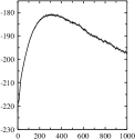
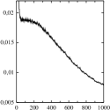
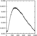
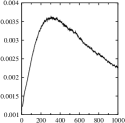
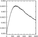
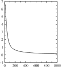
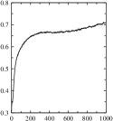
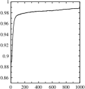
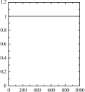
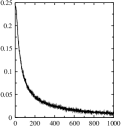
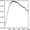
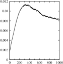
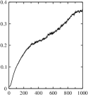
Figure 1: Results for the RAN10 problem. The first column shows the log-likelihood (top) and the reconstruction errors (7) and (8) (center and bottom). The other columns in the first, second and third rows depict $\xi_{d}$ for $D=D_{A}$, the sum of probabilities in the denominator of $\xi_{d}$ for $D=D_{A}$, and $\xi_{d}$ for $D=D_{S}$ for $d=0,1,2,3$, respectively. The x-axis is the number of epochs along the simulation divided by 50 in all plots. All data in the y-axis are in arbitrary units.

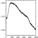
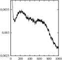
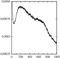
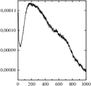
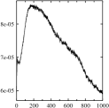
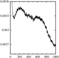
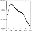
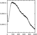
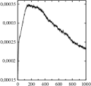
Figure 2: Results for the RAN14 problem. The first column shows the log-likelihood and the reconstruction error (7) (top and bottom panels). The other columns in the upper and lower rows show $\xi_{d}$ for $D=D_{A}$ and $\xi_{d}$ for $D=D_{S}$ for $d=0,1,2,3$, respectively.

We present the results for the problems at hand, showing for each analyzed instance different plots corresponding to the actual log-likelihood of the problem and $\xi_{d}$ for different values of $d$, among other things. In order to identify the contributions to $\xi_{d}$ from the different neighborhoods of the training set, we define two different sets: $D_{A}$ containing all states at a distance less than or equal to $d$, and $D_{S}$ accounting for those states at a distance exactly equal to $d$. We have computed $\xi_{d}$ for $D=D_{A}$ and $D=D_{S}$ in all our experiments that are commented in the following.

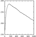
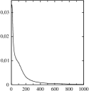
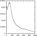
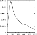
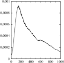
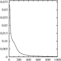
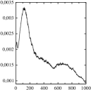
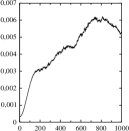
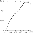
Figure 3: Same as in figure 2 for the BS data set.

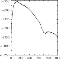
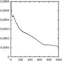
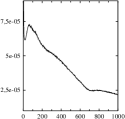
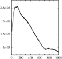
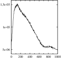
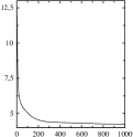
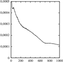
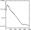
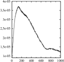
Figure 4: Same as in figure 2 for the LSE data set.

Figure 1 shows our results for the RAN10 data set. The upper left panel shows the log-likelihood of the data during training. As it can be seen, there is a clear maximum that should be identified as the stopping point. The panels below show the reconstruction errors (7) and (8) which clearly fail to identify the desired extremum. The rest of the columns show results for distances $d=0,1,2$ and $3$. The first row depicts $\xi_{d}$ for $D_{A}$, where all states at the required distances are taken into account. As it can be seen, starting at $d=1$ the criterion is robust and consistently detects the maximum of the log-likelihood at the right place, thus reinforcing the idea that the neighborhood of the data contains valuable information. The second row shows the denominator of $\xi_{d}$ corresponding to the first row, that is, the sum of probabilities of the states included in each case. Notice that for $d=3$ this sum equals one and $\xi_{d}$ is exactly equal to the likelihood of the data. More interestingly, even when the sum is still far away from one, as it happens for $d=1$, $\xi_{d}$ consistently finds the desired point. This behavior is also observed in the rest of the data sets analyzed. Finally the third row shows $\xi_{d}$ for $D_{S}$, thus showing the behavior of the criterion applied to different shells. For $d=1$ and $2$ the criterion detects reasonably well the maximum of the log-likelihood and can be used to identify the desired stopping point. Notice, though, that the data alone, entirely contained at $d=0$, is not capable to reproduce this behavior. Moreover, for $d$ larger than $2$ the criterion also fails, as it is expected that starting at a certain distance the information regarding the model is lost. Please notice that the initial transitory behavior of some of the plots above is meaningless and can be omitted so it has been cut.

Equivalent results for the RAN14 case are shown in figure 2. The log-likelihood and the probabilistic reconstruction error in (7) are depicted in the upper and lower panels in the first column, respectively. The other panels show $\xi_{d}$ for $D_{A}$ and $D_{S}$, with $d=0,1,2,3$ (top and bottom rows, second to fifth columns). As in the previous case, the reconstruction error fails to detect the maximum of the likelihood, thus not being very useful in the present context. On the contrary, a stopping point obtained from $\xi_{d}$ selects a near-optimal model. Notice that the criterion is robust along all distances explored, as desired. Similar results are found for the RAN12 and RAN16 cases. As it can be inferred from these results, the optimal value of $d$ can not be fixed beforehand and is problem-dependent.

The same plots for the BS and LSE problems are found in figures 3 and 4. Once again, the reconstruction error decreases monotonously and is therefore useless in the present context, while $\xi_{d}$ for $d$ larger than 1 successfully does the task for $D=D_{A}$, while for $D=D_{S}$ the criterion does not work in the BS problem.

Data Set	Hamming Distance
	1	2	3	4	5	6	7	8	9	10
Bars and Stripes	480	3216	11360	20744	19296	8688	1632	90	-	-
Labeled Shifter Ensemble	8434	41160	110326	165088	132976	54160	10368	966	40	2

TABLE I: Number of neighbors at different Hamming distances for the BS and LSE data sets.

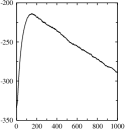
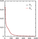
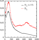
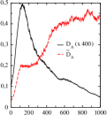
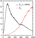
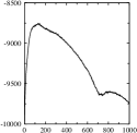
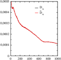
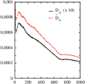
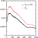
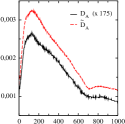
Figure 5: Comparison between $\xi_{d}$ (black curves) and $\tilde{\xi}_{d}$ (red curves) for the BS and LSE data sets (upper and lower rows). Notice that since the magnitude of these parameters is irrelevant, some curves have been scaled for the sake of clarity. The first column plots the log-likelihood of the data along the simulation.

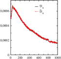
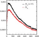
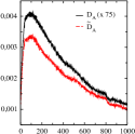
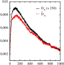
Figure 6: Same as in figure 5 for the LSE problem in CD₁₀.

IV-B Uncomplete Neighborhoods

Despite the success of the criterion built as proposed, it is clear that for large spaces it can be unpractical if the number of states in the neighborhood of the training set is very large. For that reason, we have tested the criterion on randomly selected subsets $\tilde{D}_{A}\subset D_{A}$ of the same size as the training set, which is always computationally tractable. In this sense, we denote by $\tilde{\xi}_{d}$ the evaluation of $\xi_{d}$ on $\tilde{D}_{A}$. Figure 5 shows $\tilde{\xi}_{d}$ compared with $\xi_{d}$ from the previous figures for the BS (first row) and LSE (second row) problems. More precisely, the first column shows the log-likelihood of the data along the training process, while the rest of the columns plot both $\tilde{\xi}_{d}$ and $\xi_{d}$ for $d=0,1,2$ and $3$. Notice that the absolute scales of $\xi_{d}$ and $\tilde{\xi}_{d}$ may vary mainly due to the value of the sum of probabilities in the denominators. However, since the precise value of these quantities is irrelevant, we have decided to scale them properly for the sake of comparison. Although $\tilde{\xi}_{d}$ is built from a much smaller set than $\xi_{d}$, it captures all the significant features of $\xi_{d}$ and can therefore be used instead of it. In this sense, $\tilde{\xi}_{d}$ provides a good stopping criterion for CD₁, although it is not as robust as $\xi_{d}$ due to the strong reduction of states contributing to $\tilde{\xi}_{d}$ as compared with those entering in $\xi_{d}$. This reduction is illustrated in table I, where we show the number of neighboring states to the data set at different distances for the BS and LSE problems. By increasing the number of states included in $\tilde{\xi}_{d}$, convergence to $\xi_{d}$ is expected at the expense of an increase in computational cost. However, the present results indicate that, at least for the problems at hand, a number of examples similar to that of the training set in the evaluation of $\tilde{\xi}_{d}$ is enough to detect the maximum of the log-likelihood of the data.

All the results presented up to this point show the goodness of the proposed stopping criterion for learning in CD₁. However, the underlying idea can be applied to different learning algorithms that try to maximize the log-likelihood of the data. In this way we have repeated all the previous experiments for CD₁₀ with very similar results to the ones above. As an example, figure 6 shows the log-likelihood, $\xi_{d}$ and $\tilde{\xi}_{d}$ with $d=0,1,2,3$ and CD₁₀ for the LSE data set, which is the largest one analyzed in this work. As it is clearly seen, the quality of the results is very similar to the CD₁ case, thus stressing the robustness of the criterion.

As a final remark, we note that for the BS problem the trained RBM stopped using the proposed criterion is able to qualitatively generate samples similar to those in the training set. We show in figure 7 the complete training set (two upper rows) and the same number of generated samples (two lower rows) obtained from the RBM trained with CD₁ and stopped after 5000 epochs, around the maximum shown by $\tilde{\xi}_{d=1}$, which approximately coincides with the optimal value of the log-likelihood. It is important to realize that, ultimately, the quality of the model is a direct measure of the quality of CD₁ learning, and that the model used to generate the plots is the one with largest $\tilde{\xi}_{d}$, which is quite close to the one with largest likelihood.

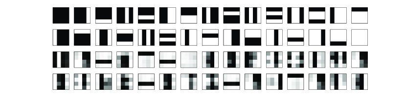
Figure 7: Training data (two upper rows) and generated samples (two lower rows) for the BS problems with the weights and bias obtained at the stopping point detected by $\tilde{\xi}_{d}$ with $d=1$.

V Conclusions

In this work we have introduced the contribution of neighboring points to the training set to build a stopping criterion for learning in CD₁. We have shown that not only the training set but also the neighboring states contain valuable information that can be used to follow the evolution of the network along training.

Based on the fact that learning tries to increase the contribution of the relevant states while decreasing the contribution of the rest, continuity and smoothness of the energy function assigns more probability to states close to the training data. This is the key idea behind the proposed stopping criterion. In fact, two different but related estimators (depending on the number of states used to compute them) have been proposed and tested experimentally. The first one includes all states close to the training set, while the second one takes only a fraction of these states as small as the size of the training set. The first estimator is robust but may require from the use of a forbiddingly large amount of states, while the second one is always tractable and captures most of the features of the first one, thus providing a suitable stopping learning criterion. This second estimator could be used in larger data set problems, where an exact computation of the log-likelihood is not possible. Additionally, the main idea of proximity to the training set will be explored in other aspects related to learning in future work.

References

- [1] H. Schulz, A. Müller, and S. Behnke, “Investigating Convergence of Restricted Boltzmann Machine Learning,” in NIPS 2010 Workshop on Deep Learning and Unsupervised Feature Learning, 2010.
- [2] A. Fischer and C. Igel, “Empirical Analysis of the Divergence of Gibbs Sampling Based Learning Algorithms for Restricted Boltzmann Machines,” in International Conference on Artificial Neural Networks (ICANN), vol. 3, 2010, pp. 208–217.
- [3] D. E. Rumelhart, G. E. Hinton, and R. J. Williams, “Learning Internal Representations by Error Propagation,” in Parallel distributed processing: Explorations in the microstructure of cognition, Volume 1: Foundations, D. E. Rumelhart, J. L. McClelland, and the PDP research group., Eds. MIT Press, 1986.
- [4] Y. Bengio, “Learning deep architectures for AI,” Foundations and Trends in Machine Learning, vol. 2, no. 1, pp. 1–127, 2009.
- [5] G. E. Hinton, S. Osindero, and Y. Teh, “A Fast Learning Algorithm for Deep Belief Nets,” Neural Computation, vol. 18, no. 7, pp. 1527–1554, 2006.
- [6] G. E. Hinton and R. R. Salakhutdinov, “Reducing the Dimensionality of Data with Neural Networks,” Science, vol. 313, no. 5786, pp. 504–507, 2006.
- [7] H. Larochelle, Y. Bengio, J. Lourador, and P. Lamblin, “Exploring Strategies for Training Deep Neural Networks,” Journal of Machine Learning Research, vol. 10, pp. 1–40, 2009.
- [8] H. Lee, R. Grosse, R. Ranganath, and A. Y. Ng, “Convolutional Deep Belief Networks for Scalable Unsupervised Learning of Hierarchical Representations,” in International Conference on Machine Learning, 2009, pp. 609–616.
- [9] Q. V. Le, M. A. Ranzato, R. Monga, M. Devin, K. Chen, G. S. Corrado, and A. Y. Ng, “Building High-level Features Using Large Scale Unsupervised Learning,” in 29th International Conference on Machine Learning, 2012.
- [10] P. Smolensky, “Information Processing in Dynamical Systems: Foundations of Harmony Theory,” in Parallel Distributed Processing: Explorations in the Microstructure of Cognition (vol. 1), D. E. Rumelhart and J. L. McClelland, Eds. MIT Press, 1986, pp. 194–281.
- [11] S. Geman and D. Geman, “Stochastic Relaxation, Gibbs Distributions, and the Bayesian Restoration of Images,” IEEE Transactions on Pattern Analysis and Machine Intelligence, vol. 6, no. 6, pp. 721–741, 1984.
- [12] G. E. Hinton, “Training Products of Experts by Minimizing Contrastive Divergence,” Neural Computation, vol. 14, pp. 1771–1800, 2002.
- [13] Y. Bengio, P. Lamblin, D. Popovici, and H. Larochelle, “Greedy Layer-wise Training of Deep Networks,” in Advances in Neural Information Processing (NIPS’06), vol. 19. MIT Press, 2007, pp. 153–160.
- [14] Y. Bengio and O. Delalleau, “Justifying and Generalizing Contrastive Divergence,” Neural Computation, vol. 21, no. 6, pp. 1601–1621, 2009.
- [15] M. A. Carreira-Perpiñán and G. E. Hinton, “On Contrastive Divergence Learning,” in International Workshop on Artificial Intelligence and Statistics, 2005, pp. 33–40.
- [16] A. Yuille, “The Convergence of Contrastive Divergence,” in Advances in Neural Information Processing Systems (NIPS’04), vol. 17. MIT Press, 2005, pp. 1593–1600.
- [17] D. J. C. MacKay, “Failures of the one-step learning algorithm,” 2001, unpublished Technical Report.
- [18] T. Tieleman, “Training Restricted Boltzmann Machines using Approximations to the Likelihood Gradient,” in 25th International Conference on Machine Learning, 2008, pp. 1064–1071.
- [19] T. Tieleman and G. E. Hinton, “Using Fast Weights to Improve Persistent Contrastive Divergence,” in 26th International Conference on Machine Learning, 2009, pp. 1033–1040.
- [20] G. Desjardins, A. Courville, Y. Bengio, P. Vincent, and O. Delalleau, “Parallel Tempering for Training of Restricted Boltzmann Machines,” in 13th International Conference on Artificial Intelligence and Statistics (AISTATS), 2010, pp. 145–152.
- [21] G. E. Hinton, “A Practical Guide to Training Restricted Boltzmann Machines,” in Neural Networks: Tricks of the Trade. Springer, 2012, pp. 599–619.
- [22] R. M. Neal, “Annealed Importance Sampling,” 1998, technical Report 9805, Dept. Statistics, University of Toronto.
- [23] R. Salakhutdinov and I. Murray, “On the Quantitative Analysis of Deep Belief Networks,” in International Conference on Machine Learning, 2008, pp. 872–879.
- [24] E. Aarts and J. Korst, Simulated Annealing and Boltzmann Machines. A Stochastic Approach to Combinatorial Optimization and Neural Computing. John Wiley, 1990.
- [25] A. Fischer and C. Igel, “Training Restricted Boltzmann Machines: An Introduction,” Pattern Recognition, vol. 47, pp. 25–39, 2014.
- [26] P. Bühlmann and S. Van De Geer, Statistics for High-dimensional Data: Methods, Theory and Applications. Springer Science & Business Media, 2011.