Small-angle scattering behavior of thread-like and film-like systems
Abstract
Film-like and thread-like systems are respectively defined by the property that one of the
constituting homogenous phases has a constant thickness () or
a constant normal section (of largest chord ). The stick probability
function of this phase, in the limit , naturally leads to the
definition of the correlation function (CF) of a surface or of a curve. This CF
fairly approximates the generating stick probability function in the
range of distances larger than . The surface and the curve
CFs respectively behave as and as as
approaches to zero. This result implies that the
relevant small-angle scattering intensities
behave as or as in an intermediate range
of the scattering vector () and as in the outermost
-range. Similarly to , pre-factors and
simply depend on some structural parameters. Depending on the scale
resolution it may happen that a given sample looks thread-like at large scale,
film-like at small scale and particulate at a finer one. An explicit example
is reported. To practically illustrate the above results, the surface and the curve CFs
of some simple geometrical shapes have been explicitly evaluated. In particular,
the CF of the right circular cylinder is explicitly evaluated. Its limits, as the height or the
diameter the cylinder approaches zero, are shown to coincide with the CFs
of a circle and of a linear segment, respectively.
Synopsis:The scattering intensities of thread-like and film-like
systems respectively behave as and in an
intermediate range of the scattering vector . The and
expressions are reported.
Keywords: film-like systems, thread-like systems, surface
correlation function, curve correlation functions, scale resolution, small-angle
scattering intensity behavior
1 Introduction
Materials characterized by one film-like or by one thread-like phase are since
long known. Examples of the first kind are vesicles in solutions or
oil-water-surfactant systems. Examples of the second kind are polymers
or amyloid proto-filaments (Avdeev et al., 2013) in solution. Small-angle
scattering (SAS) is one the most suitable tools to characterize these materials
when the film thickness or the thread diameter is of the nanometer order.
In fact, based on the knowledge that the SAS intensity [] of a circular
cylinder decreases, at intermediate scattering vector () values, as
or as depending on whether the cylinder’s radius is much larger
or much smaller then its height (Porod, 1982; Kirste & Oberthür, 1982),
one looks for the existence of a plateau in the plot of or of
versus to conclude that the sample respectively contains (plane) flat
particles or (straight) rod-like ones.
Actually this conclusion has a more general validity since
it also applies to the cases of curved film-like and thread-like phases. To the authors’
knowledge, a first attempt to get this more general result,
starting from the basic equations of
SAS theory (Guinier & Fournet, 1955; Kostorz, 1979; Feigin & Svergun, 1987),
was done by Teubner (1990) in the film-like case.
To make this derivation more detailed as well as to extend it to the thread-like
case is the aim of this paper according to the following plan.
Section 2 reports the basic definitions and results of SAS theory for
three phase samples. Section 3 considers the case where one of the
constituting phases is a film of thickness . One shows how the limit
of the stick probability function (SPF) of the film-like phase
leads to the definition of a surface correlation function
[]. This function fairly approximates the generating SPF
in the range and it behaves as at small distances.
Furthermore, the surface CF is explicitly evaluated in the case of a sphere
(§ 3.4.1), a circle (§ 3.4.2), a rectangle (§ 3.4.3) and a cubic surface
(appendix B). The circle is the limit of a right circular cylinder as the
cylinder’s height goes to zero. Hence, the corresponding limit of the cylinder
CF must coincide with that of the circle. To verify this point one needs to
know the explicit expression of the cylinder CF while the only chord-length
distribution is presently known (Gille, 2014). This CF calculation is
performed in closed form in terms of two elliptic integral functions (see
appendix A). Section 4 analyzes the case of a tread-like phase.
In the limit of vanishing thread diameter, the corresponding limit of the
relevant SPF leads to the definition of the curve correlation function
[] that behaves as as and fairly
approximates the considered SPF if . The curve CFs of a linear
segment and a circle are explicitly worked out in § 4.1.1 and § 4.1.2.
In § 4.1.1 one also shows that the linear segment CF coincides with the
limit of the cylinder CF as the cylinder’s radius goes to zero.
The behaviors of the scattering intensities relevant to film-like and thread-like
phases are discussed in § 5. The existence of an intermediate -range
where the two intensities respectively behave as
and as is proved in § 5.1 and § 5.2. Of course, both intensities
behave as in the outer -range. The analytic expressions of
pre-factors and are also worked out and three simple
illustrations are reported. In § 5.3 one discusses
the behavior of the scattering intensity of a right parallelepiped. If the sizes
of the sides differ more than two order of magnitudes, one finds that the
intensity at first behaves as , then as and finally as in agreement
with the fact that the parallelepiped looks as a thread when observed on a large scale,
as a film when the observation scale becomes smaller and, finally, as a parallelepiped when
the observation scale has become fine enough to resolve all the involved lengths.
Section 6 draws the final conclusions.
2 Basic definitions and properties of the SPFs
Consider a statically isotropic sample made up of three homogeneous phases. The th of these occupies the spatial set , of volume , and has scattering density . The total sample occupies the union set of volume . The volume fraction of the th phase is . The correlation function of the sample is given by (Ciccariello and Riello, 2007)
| (1) |
Here denotes the scattering contrast between phase and the remaining pair of phases . It is defined as
| (2) |
is the mean square scattering density fluctuation. It is equal to or to . Finally, according to the definition
| (3) |
denotes the CF of the th phase. It is determined by the only geometry of the th phase because is the stick probability function (SPF) relevant to the phase pair . The SPFs were first introduced by Debye et al. (1957) [see, also, Peterlin (1965) and Goodisman & Brumberger (1971)], in analogy with the Patterson function, according to the definition
| (4) |
Here is the characteristic function of the set (i.e. is equal to one or zero depending on whether the tip of falls inside or outside ) and denotes a unit vector that spans all possible directions. The first integral, it being an angular average, ensures the assumed isotropy of the sample. The probabilistic meaning of the SPFs defined by (4) implies (Goodisman & Brumberger, 1971) that
| (5) |
where is Kronecker’s symbol. Once the above equalities are substituted within equations (1) and (3) one finds that, whatever ,
| (6) |
Definitions (1) and (3) imply that the -dependence of the sample CF is determined by that of the SPFs that will now briefly reviewed. To this aim it is observed that the SPFs can also be written as (Ciccariello et al. 1981)
| (7) |
where , as specified by the index value, denotes the three-dimensional Dirac function. From this expression follows that the behavior of , as , mainly reflects the geometrical features of surface that separates the th phase from the remaining ones. In fact, it results that
| (8) |
where denotes the area of surface (Porod, 1951), is the total length of edges present on and, finally, , and respectively are the angularity (Méring & Tchoubar, 1968; Porod, 1967; Ciccariello, 1984), the curvosity (Kirste & Porod, 1962) and the sharpness (Ciccariello & Sobry, 1995) of the surface. These quantities are defined as follows
| (9) |
| (10) |
and
| (11) |
with
| (12) | |||
In (9), the first contribution (Ciccariello et al., 1981) refers to the edges and denotes the dihedral angle value at the edge point with curvilinear coordinate . The second contribution (Ciccariello & Benedetti, 1982) arises from possible points of contact between different branches of surface . These points are indexed by , and denotes the corresponding value of the Hessian of the function resulting from the difference of the two branches. Kirste & Porod (1962) obtained equation (10). Here and respectively denote the mean and the Gaussian curvatures of surface at the point (with position vector) . The two curvatures are related to the minimum [] and the maximum [] curvature radius of the surface by
| (13) | |||||
| (14) |
Finally, equation (11) was obtained by Ciccariello & Sobry (1995). The outer
summation there present is performed over all the vertex points of and the inner one over
all distinct triple of edges that enter into the th vertex. Further,
denotes the angle formed by the th and the th
edge while
is the dihedral angle at the th edge. It is also noted that, whenever a
couple of facets do not share a common edge but only a vertex, one has to
consider the virtual edge along which the facets, once they are prolonged,
intersect each other. This fact explains the presence in (12) of the sign
factor . One should refer to page 65 of the above paper
for the full definition. This paper also shows that the SPF of a
phase bounded by a polyhedral surface is a 3rd degree polynomial within the
innermost range of distances, i.e. it is exactly given by equation (8)
with .
A further property of SPFs is the fact that, whenever parts of the
interfaces are parallel to each other at a relative orthogonal distance ,
the second derivative of the relevant SPF shows a finite (Wu & Schmidt, 1974)
or a logarithmic discontinuity (Ciccariello, 1989) as . This
property was thoroughly discussed by Ciccariello (1991) and is practically useful
(see, e.g. , Melnichenko & Ciccariello, 2012 and references therein).
This property applies to film-like samples and yields an oscillatory contribution
decreasing as in the range . For simplicity, however, this
contribution will not explictly be considered in § 5.1.
3 Film-like phase and surface CF
Assume now that phase 1 have a film-like structure, i.e. is a connected or disconnected set delimited by a left () and a right () surface at a relative constant orthogonal distance . Moreover, one also assumes that and be smooth (i.e. they have no edges, vertices and contact points) and that be small in the sense that it obeys the inequality
| (15) |
where denotes the mean value of the curvature radii of , the surface bounding . Denote the surface midway and by . Then, , the position vector of a generic point P of , can uniquely be written as
| (16) |
where denotes the position of the point intersection of with the straight line [with direction ] that going through P, is normal to . is the orthogonal distance of P from . In equation (7) with , the infinitesimal volume element located at can be written, up to terms , as [see, e.g., equation (4.7) of Ciccariello (1991)]
| (17) |
where is the infinitesimal surface element of located at . Using equations (16), (17) and (7), one concludes that the SPF of film-like phase 1 takes the form
| (18) |
3.1 The surface CF definition
In the range of distances this function is reliably approximated by equation (8) that in the present case reads
| (19) |
since the smoothness of the surface and the smallness of makes
the surface area approximation accurate.
In the range , the smallness of makes it possible to
set within the integrand of (18) so that the SPF becomes
| (20) |
with
| (21) |
Function is named surface
correlation function because it is fully determined by the surface set . Function
was first introduced by Teubner (1990). [Note, however,
that this author used , instead of , as normalization
factor in front of the integral reported in (21).]
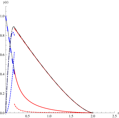
Figures 1 and 2 show the accuracy achieved in approximating the
bulk SPF by the 3rd degree -polynomial (19) in the range
and by the surface CF, via equation (20), in the range
for two simple particle shapes: the spherical shell and the cylindrical disk. The
accuracy drastically improves as gets smaller.
3.2 Properties of the surface CF
From equation (20) and the fact that is dimensionless it follows that the surface CF has dimension length-1. The leading behavior of the surface CF as was obtained by Teubner (1990), under the assumption that the surface is closed [i.e., with no boundary] and smooth, by the same procedure that Kirste & Porod (1962) followed to get their relation. It reads
| (22) |
where the angular brackets denote the average over .
This relation shows that the surface CF diverges as so that it cannot be
normalized to one at the origin as it happens for standard CFs.
As , the leading behavior of the surface CF is
| (23) |
This immediately follows from equations (5) and (20) since
It is also noted that the surface CF defined by equation (21) generalizes the two dimensional (2D) CF defined as (Ciccariello, 2009)
| (24) |
where is a plane set and is a unit vector that spans the unit circle. To get the relation between the two quantities in the case where the set, present in (21), is plane, one chooses the plane where lies as the plane. Then, in (21) one writes
[where is the projection of onto the plane] and, after integrating over , one gets
| (25) |
where the outermost integral is performed on the unit circle. Comparing (25) with (24) and assuming that one finds
| (26) |
Ciccariello (2010) showed that, as , where denotes the length of the boundary of . Thus, relation (26), allows us to generalize equation (22) to the case where is an open surface, and has therefore a boundary of perimeter , in the following way
| (27) |
Finally it is observed that the moments of the surface CF can be expressed in terms of the moments of the surface if . . In fact, putting
| (28) |
from equation(21) follows
The last expression is equal to the sum of products of different moments of surface [see appendix B of Ciccariello (2014)]. In particular, if , one simply finds
| (30) |
3.3 Integral expressions of the derivatives of the surface CF
The comparison of (21) with equation (3.1) of Ciccariello et al. (1981) shows that the surface CF and the second derivative of nearly have the same mathematical structure since the only difference, aside from the normalization factors, lies in the angular contribution that is only present in the expression. Consequently, many of the elaborations worked out for this expression apply, mutatis mutandis, to the surface CF. In particular, let denote the spherical surface with center at and radius . Then equation (21) can be written as
| (31) |
Omitting the overbar, denoting by the intersection curve of with (it is formed by the points of that are at distance from point of ) and proceeding as in the just mentioned paper, one finds that takes the form
| (32) |
In this expression, is the curvilinear coordinate of the curve points
(note that the curvilinear coordinate definition is such that the distance
between two points, having curvilinear coordinates and ,
is equal to ), denotes the unit vector
orthogonal to (and pointing outwardly to) at the
point and specifies the direction
of the vector .
If one puts
| (33) |
and
| (34) |
equation (32) becomes
| (35) |
Thus, is proportional to that denotes the average value of over . The th derivative of takes the form
| (36) |
which implies that the reduced integral expressions involve an integration, along the same curve, of an integrand that changes with the derivative order . To get the integrand expression, proceeding as in Ciccariello (1995), one denotes by the parametric equation of , and by and the corresponding derivatives with respect to and . One puts
| (37) |
[where and denotes the unit vector tangent to at ] and
| (38) |
where the reported partial derivatives are evaluated at the argument values shown on the left hand side. In this way, the integral expression of the th derivative of the surface CF becomes
| (39) |
under the assumption that the involved partial derivatives exist.
3.4 Examples of surface CFs
The following subsections report the surface CFs relevant to a spherical surface, a circle and a rectangle, while the surface CF of a cubic surface is worked out in appendix B.
3.4.1 The CF of spherical surface
Consider a spherical shell of inner and outer radius equal to and with . The bulk CF was calculated by Glatter (1982) (see also Fedorova & Emelyanov, 1977) and reads
| (40) |
with .
As , the spherical shell becomes a spherical surface of radius R.
The corresponding CF is easily evaluated by (35). In fact,
is a circle of radius and .
In this way, from (35) follows that
| (41) |
This expression is equal to as required by equation (20). Figures 1a and 1b allows one to appreciate the accuracy achievable in approximating by for the cases u and u, respectively.
3.4.2 The surface CF of a circle
Consider a circular cylinder of radius and height . If one lets go to zero, the cylinder shrinks to a circle of radius . The surface CF of the circle is easily evaluated by equation (26). In fact the value of the 2D CF of a circle at a given distance is proportional to the overlapping area of the outset circle and the circle shifted by . In this way, accounting for the appropriate proportionality constant, one finds that the surface CF of a circle is
| (42) |
One easily verifies that
where denotes the cylinder CF that is given by (108). Besides, the small distance expansion of (42) yields
| (43) |
in agreement with equation (27).
Similarly to Fig. 1, Fig. 2 shows the accuracy achieved in
approximating , the cylinder CF, by the relevant
polynomial within the range and by
if in the case where
the cylinder has height equal to u and radius equal to u.
3.4.3 The surface CF of a rectangle
Consider a rectangle of sides and with . Its surface CF is easily obtained using equation (26) and recalling that the 2D CF of any plane polygon has an algebraic form (Ciccariello, 2009). Hence, using the result of this paper, one finds that the surface CF of the aforesaid rectangle is
| (44) |
4 Thread-like phase and curve CF
Consider now the case where one of the sample phases (named again phase 1) is formed by threads having the same normal section of maximal chord and area . Assume that be small (in a sense that will be defined later). Then, in the limit , phase 1 shrinks to a curve that might have branching points. The number of these points is assumed to be negligible. The curve can be parameterized as
| (45) |
where denotes the curvilinear coordinate of the curve point set at . It is also assumed that is smooth in the sense that is continuously differentiable up to the third order (included). Then, the curve at each of its points is endowed of two curvature radii: and , respectively named curvature radius and torsion radius (Smirnov, 1970). To define these, one considers the three mutually orthogonal unit vectors defined as follows
| (46) |
and respectively named tangent, normal and binormal vectors. Clearly, specifies the direction of the tangent to at , is the unit vector orthogonal to such that these two vectors determine the plane osculating the curve at . Besides, the orientation of is such that the curve looks concave at the considered point. The expressions of the aforesaid radii are as follows
| (47) |
The curvature radius is the radius of the circumference osculating the curve while
the torsion radius specifies how the osculating plane rotates as one moves
along the curve. It follows that the curvature radius is always positive while the
torsion radius can be positive at some points of the curve and negative at others.
Similarly to equation (15) one defines the mean of the curvature radii of
the curve as
| (48) |
where the average is performed integrating all over the length of .
(It is noted that generally consists of many disjoint closed and/or open
curves.)
One goes now back to , the SPF of the thread-like
phase, to analyze in more detail the limit . First, it is observed
that is small if as it will hereafter be assumed. Let
be the position vector of a point of phase 1 and consider the plane that
contains this point and is orthogonal to . Denote respectively by and by
the intersections of the plane with and with the
thread-like phase. One can then write where
lies within , the normal section set of the thread at .
Function can be written as
| (49) | |||
The volume fraction of the thread-like phase is fairly approximated by with equal to the total length of the threads. From equation (5) follows that
| (50) |
Similarly to the case discussed in § 3.1, in the range , is fairly approximated by equation (19). This can be written in the algebraic form
| (51) |
if one approximates the
threads by circular cylinders so that ,
and .
In the range , owing to the smallness of , one can neglect
the dependence on and within the Dirac function. Then,
the integrals over these variables can explicitly be performed and one finds that
| (52) |
with
| (53) |
One concludes that the -dependence of the SPF of a thread-like phase is
described by function in the outer distance range and by
equation (51) in the inner one.
Function is determined by curve and will
be named curve correlation function. The dimensions of
are .
First one elaborates equation (53) so as to convert it into a one dimensional
integral. To this aim, the equation is written as
| (54) |
where denotes the position vector of the infinitesimal surface element of , the sphere of radius centered at the infinitesimal curve element set at . Note that the modulus of is . One denotes the function defined by the innermost two integrals of (54) as
| (55) |
The function can easily be evaluated choosing a Cartesian orthogonal frame having the origin at the position of so that . The value of the integral can be different from zero if and only if intersects . Assume that the intersection points exist and let denotes one fo these points. Then, one chooses the axis along . The plane containing is perpendicular to while forms an angle, denoted by , with axis , so that . Around , takes the form and its value is . Recalling that is parallel to , with defined by equation (46a), one gets
| (56) |
| (57) |
and
| (58) |
where index labels all the points of that are at distance from the point set at . It is stressed that equation (56) determines the direction of as well as the curvilinear coordinate value (denoted by ) owing to the fact that the vector on the right side of (56) must be unimodular. By (54) and (58) one concludes that the curve CF is proportional to the curvilinear average of , i.e.
| (59) |
The leading asymptotic behavior of the above expression as is worked out in appendix C and reads
| (60) |
This result shows that the curve CF diverges as as one approaches the origin. The leading behavior of the curve CF as is immediately obtained by equations (52) and (50b) and reads
| (61) |
The moments of the curve CF, similarly to the case of the surface CF, can be expressed in terms of the moments of the curve. In fact
| (62) |
From this relation follows that .
4.1 Examples of curve CFs
Two examples of curve CFs are reported in the following subsections.
4.1.1 The curve CF of a linear segment
The first refers to a linear segment of length . Applying definition (54), the angle defined by (57) is equal to zero. Thus, equation (59) yields
| (63) |
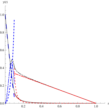
By letting the radius of a circular cylinder go to zero, the limit of its CF [multiplied by as required by (52)] must reproduce (63). One easily checks that this property holds true evaluating the aforesaid limit stemming from , the cylinder CF given by equation (109). Besides this CF can be approximated by (51) if and by if . Fig. 3 shows the achieved accuracy in the case u and u.
4.1.2 The curve CF of a circumference
The curve CF of a circumference of radius also can easily be evaluated. One puts . Given , the associated value is . Then one finds that so that . Finally, from (59), one gets the circumference CF
| (64) |
This CF behaves as as and diverges as as .
5 Scattering intensity behavior
The scattering intensity is the Fourier transform (FT) of equation (1) times and is, therefore, equal to
| (65) |
This can be recast into the form (Ciccariello& Riello, 2007)
| (66) |
with
| (67) |
The existence of the integral is ensured by condition (6b), while equation (6a) implies the following sum-rule
| (68) |
responsible for the Porod invariant relation
| (69) |
Besides, the s obey the condition
whatever the scattering vector because
they are the FTs of the s that have a convolution structure
owing to definitions (3) and (4). However, these conditions
are not sufficient, on the basis of (65), to ensure the required
positiveness of because some of the s can be negative.
Hence, the last quantities have to obey appropriate constraints to ensure
the positiveness of . This conclusion, that might look at first
surprising, is a consequence of the functional density theorem that
states that the correlation function is uniquely determined by the
density value and the interaction potential. On the basis of this
statement it is clear that the assignment of the sample internal geometry,
equivalent to assigning the s, cannot be fully
independent of the values.
Each is determined by the length distribution of the
chords that have both ends within the related phase. In most of
the cases the distribution is not uniform but has a particular shape that
naturally defines some length values as the bounds
of the ranges relevant to the small and the large distances asymptotic
behaviors of as well as to the positions of possible peaks and
shoulders. Since is obtained from by sutracting
to this quantity it happens that is certainly
positive around the origin owing to (6a) and that it can be negative
for other values. The aforesaid distances
in turns define some particular scattering vector
values through the well known relation
. The s are the reciprocal space values
where one expects a change in the behavior.
One applies now these considerations to the film-like and thread-like
systems discussed in the previous sections. There it was shown that the
SPF is certainly endowed of two typical lengths:
[] [see equations (15) and (48)] and
with [] and that
is fairly approximated by a third degree polynomial if
and by a surface [a curve] CF if
. It is convenient to separately discuss the case of
film-like systems and that of thread-like ones.
5.1 Intensity behavior in the film-like case
To begin with one analyzes first the behavior of under the further simplifying assumption that one only has two typical lengths,i.e. and . Thus, the behavior is expected to change as one passes from the -range to and, finally, to . By (3) and the results of § 3 one finds that
| (70) |
where it has been put
| (71) |
The FT of equation (70) yields
| (72) |
with
| (73) |
and
| (74) |
[It is observed that condition (23) ensures that as so that integral (74) exists.] The behavior of within the first -range could be obtained by expanding the function around . One finds
| (75) |
with
| (76) |
and
| (77) |
One sees that is
the th moment of . Since is
, the value of is essentially equal to the
corresponding momentum of and strongly
depends on the way approaches zero as
. Since the last behavior generally is not known, on a general
ground the only existence and positiveness of is certain. The
existence of the other higher moments is certain only if one assumes that
approaches zero by an exponential decrease
or, more strongly, that the sample is a dilute collection of particles with
a finite maximal size and that the inter-particle interference may be
neglected (Guinier & Fournét, 1955).
Consider now the second -interval . If is
close to , contribution to
can still, though less accurately, be approximated
by the sum
[see (75)]. To estimate contribution
one must determine its asymptotic behavior as . Integrating
equation (74) by parts one finds that the leading term is
In this expression, the contribution related to is canceled by the corresponding contribution present in since also presents the constant term . Thus one can write
| (78) |
provides one also writes
| (79) |
where the primes denote that the moments have been evaluated by (75) without subtracting from . In the sub-interval of the considered -range such that and , using (22) and the relation , from (78) one gets
| (80) |
Recalling that is one finds that that, compared to the above contribution, can be neglected. One concludes that
| (81) |
Once one considers the third -range, i.e. , in direct space the sample structure is analyzed on a distance scale smaller that . Then, the limit is no longer valid and the large behavior of must be determined starting from the FT of defined by (3). An integration by parts and the use of (8) immediately yields the equivalent of the Porod relation
| (82) |
Confining oneself to three phase film-like systems where film-like phase 1 fully separates phase 2 from phase 3 (so that the last two phases have no common interface), phases 2 and 3 are characterized by the only length . Then, by the same considerations that yielded (82), one concludes that the asymptotic leading terms of and are
| (83) |
Substituting the above asymptotic behaviors within equation (65) it results that the asymptotic leading term of the scattering intensity relevant to a three-phase film-like system (with no common interface between phases 2 and 3) is
| (84) |
with
| (85) | |||||
| (86) |
The main conclusion of this analysis is that: if , the log-log
plot of the scattering intensity of a three-phase film-like system shows a linear
behavior with slope -2 at intermediate -values and a further linear
behavior with slope -4 in the outer -range (of course, provided ,
the largest observed scattering vector, obeys to ).
Hence, the lower bounds and of the two linear behavior ranges
yield an estimate of and through the relations
and . The intersections of
the two straight lines with the vertical axis set at determine
the values of and .
According to (85) and (86), the resulting ratio
determines if the phase contrasts are known and then, either
or can be used to determine the film area .
The assumption that phases 2 and 3 have no common
interface is now relaxed. Then, equations (81) and (82)
remain unchanged while the second of equations (83) converts into
| (87) |
and a similar one for with . From these relations and (65) one obtains the general expressions of and
| (88) | |||||
| (89) |
Though these two relations, even combined with the Porod invariant one, are no longer sufficient
to determine the four structural parameters and , they yield
however useful general bounds on these parameters.
Two illustrations are now reported. Although they are naïve mathematical
models they illustrate the main points of the previous discussion. The first
illustration deals with the scattering intensity of a spherical shell whose
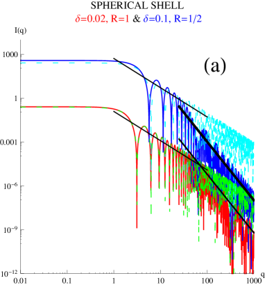
parameters take the values: (1, 0.02)u and (0.5, 0.1)u. The left panel of Fig. 4 shows, in red and blue, the spherical shells’ scattering intensities obtained by the FT of (40) and, in cyan and green, the corresponding FTs of [see (41)], equal to
| (90) |
[This FT has been obtained by integrating over , the total support of .]
The thin and the thick continuous straight lines are the plots of the leading
asymptotic terms given by equation (84) [and (85) and
(86)]. The figure shows that the intensity relevant to the spherical
shell [leaving aside the oscillations] shows both a and a
behavior and that the intensity of the associated spherical
surface well reproduces the first intensity throughout the range
(i.e. not only within ). Moreover it results that
the smaller the ratio the wider becomes the range where the
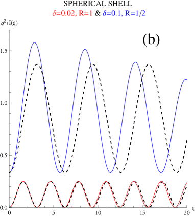
behavior occurs. The right panel of Fig. 4 shows the versus
plots (also known as Kratky plots) of the two considered spherical shells
(continuous curves) and of their associated spherical surfaces (broken curves).
The agreement is much better in the case (1, 0.02) owing to the smaller
value.
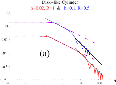
The second illustration deals with the case of two disk-like cylinders characterized by u and u. The corresponding intensities are obtained by numerically Fourier transforming equation (108) and respectively yield the red and the blue continuous curves shown in Fig. 5a. The associated surface-like intensities are the 3D FTs of (42) multiplied by , i.e.
| (91) |
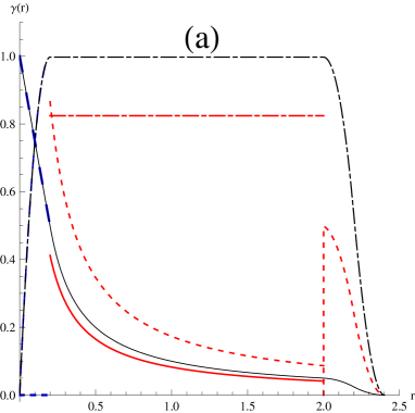
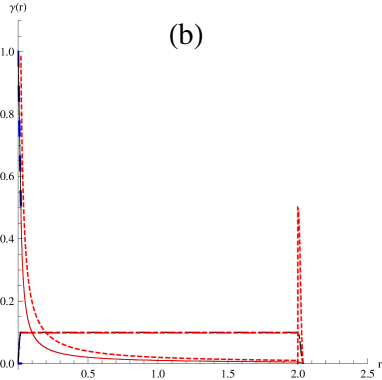
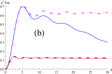
Their plots are shown as magenta and purple broken curves. They practically superpose to the red and blue curves throughout . The black lines are the plots of the relevant leading asymptotic behaviors given by (84). One again observes that the -range, where the intensity behavior is becomes wider as decreases. In the outer range, as expected, the surface approximation no longer works since the intensity behaves as in agreement with Porod’s law. Fig. 5b allows one to better appreciate how the agreement between the particle and the surface-like intensities improves throughout as decreases.
5.2 Intensity behavior in the thread-like case
Though, in most cases, a thread-like phase exists in presence of another single phase, hereafter one assumes that it exists in presence of two further phase and that the thread-like phase portion that lies on the interface between phases 2 and 3 is negligible so as to have , where and respectively denote the total lengths of the threads that fully lie within phases 2 and 3. It is also assumed that
| (92) |
and that the mean of the curvature radii of is not smaller than , defined by (48). The above assumptions amount to say that the threads are in an extended configuration and that the mean distance among them is not smaller than . These properties make it possible to apply the considerations made in § 5.1 to the thread-like case. Thus, the equation equivalent of (74) and (71b) becomes
| (93) |
By (60), considering the only leading term, one finds
| (94) |
where is the sine integral function (Gradshteyn & Ryzhik, 1980) that, at small , behaves as . One concludes that
| (95) |
In this -range the s with are negligible since they are . In the range the behaviors are similar to those found in the film-like case. One finds
| (96) |
and
| (97) |
By (95), (96), (97) and (65) the asymptotic behavior of the thread-like scattering intensity is
| (98) |
with
| (99) |
and given by (89).
The main consequence of this analysis is that the log-log plot of
the scattering intensity of a thread-like sample may show a linear behavior
with slope -1 at intermediate values and another linear behavior with
slope -4 (i.e. the Porod one) at larger s. The associated constants
and are related to the the section and the length of
the thread-like phase, the scattering contrasts and the interface surface
areas as reported in (99) and (88). The expressions
immediately convert to the two phase case ones by setting
and . In this way the expression reduces to that
obtained by Kirste & Oberthür (1988) under the more restrictive
assumption that the particles are rod-like. In particular, in the two phase
case, the determination of and allows one to determine
the normal section and the total surface areas of the thread-like phase if
one knows the contrast because volume fraction can be obtained
by the Porod invariant value [i.e. equation (69)].
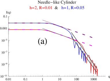
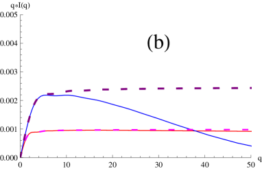
Figure 6 reports an illustration of these results considering the
case of a needle-like cylinder, i.e. a cylinder with its height larger
than is diameter . The scattering intensity is obtained by the numerical
integration of (109). The intensity associated to the limit
of the thread like phase is obtained, according to (52), multiplying
by the FT of (63). In this way one finds
| (100) |
where is the sine integral function. The expression on the right hand side approaches as and behaves as in the range . The figure shows that the region where the intensity behaves as enlarges as the ratio decreases. Actually, as in the previously reported cases, this value must be smaller than few percents for the behavior to be clearly observed.
5.3 The right parallelepiped case
It may happen that a given sample appears as made up of threads if observed on a coarse length scale and of films if observed on a fine one. Then, its scattering intensity will show both a and a behavior, besides the one at very large s. A dilute monodisperse and statistically isotropic sample made up of right parallelepipeds of sizes with , is a paramount example of this phenomenon, as it will now be shown. The monodispersity assumption allows one to confine the attention to the behaviors of the CF and the form factor of a single parallelepiped. The CF of this particle shape was worked out by Gille (1999) and has an analytic form. Since one expects that the parallelepiped looks as a linear segment on a length scale greater than (and smaller than ) and as a rectangle on a scale greater than (and smaller than ), from equations (52) and (20) it follows that
| (101) |
where is the parallelepiped CF reported by Gille (1999), the linear segment CF given by (63) and the rectangle surface CF given by equation (44).
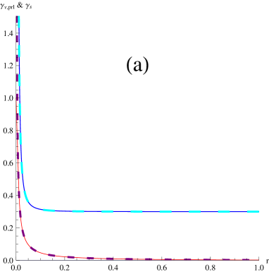
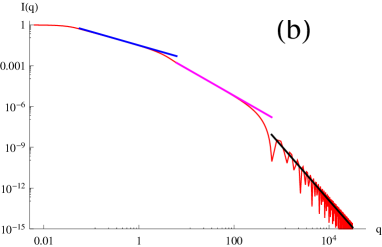
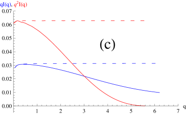
Figure 8a shows the accuracy achieved by (101) in approximating the CF of a right parallelepiped with u, u and u by the relevant film and thread CFs. In fact, the continuos red curve is the plot of and the broken magenta one that of throughout the range . The continuous blue curve is the plot of and the broken cyan one that of throughout (this interval has been linearly mapped over [0.01, 1], and both curves are vertically shifted by 0.3). The form factor of the considered parallelepiped is the red curve shown in fig. 8b and is numerically obtained evaluating the FT of . The blue, the magenta and the black linear segments, which respectively behave as , and , have been obtained by equations (98a), (84a) and (98b) [or (84b)]. They have been drawn within the -ranges: , and . One sees that the and behaviors are fairly obeyed close to the lower bounds of the previous two intervals. In the proximity of the two upper bounds, the intensity deviates from the reported two linear behaviors as it appears more evident in figure 8c. Here the continuous and broken blue are the plots of and of [note that, similarly to the previously reported cases, this FT has been evaluated integrating over the full support of to ensure its positiveness] within the -range, and the continuous and broken red curves are the Kratky plots of and the FT of (evaluated over within (the last interval has been linearly mapped over the former one).
6 Conclusion
The reported analysis has shown that the CF of a thread-like or a film-like statistically isotropic sample can be approximated by a 3rd degree polynomial in an inner distance range and, externally to this, by the associated curve or surface CF. The curve and the surface CFs respectively behave as and as close to the origin. Consequently, the relevant scattering intensities respectively behave as or as in a range of intermediate s and as in the outer range. The and expressions were determined by Porod (1951) and by Teubner (1990). The expression of is new. Both and coincide with the expressions obtained by Porod (1982) and by Kirste & Oberthür (1982) in the cases of plane lamellae and circular rods. On a practical ground, coefficients and or can easily be determined from the linear portions of the intensity log-log plot. Their knowledge determines, in a (nearly) model independent way, the interface area as well as the normal thread section area or the film thickness. Furthermore, a numerical check on the physical consistency of the assumed film-like or thread-like structure is possible because the lower bound of the -range where the or behavior occurs must be close to the film thickness value or to the thread maximal chord value (estimated from the normal section area), respectively determined by and . The model illustrations, reported in § 3.4.1, 3.4.2 and 4.1.1, suggest that the linear behaviors in the log-log plots are observable if the two typical lengths, and for the film-like case and and for the thread-like one, differ at least by an order of magnitude. This fact is confirmed by Figures 5 and 6. The paper analysis also applies to three phase systems. In thie case of film-like samples involving three phases, the knowledge of coefficients , and only puts some bounds on the involved structural parameters since it is not sufficient to uniquely determine them. Whenever the scattering intensity is collected over a wider -range, as it happens using also ultra-small scattering equipments, one might study samples that behave in a thread-like way in the innermost -range and in a film-like one in the intermediate -range (see the model illustration reported in § 5.3). In this case, a trivial extension of the above analysis makes it possible to determine both the thread section area and the film thickness of the analyzed sample.
Appendix A: the circular cylinder CF
The chord length distribution (CLD) of a circular right cylinder of radius and
height is since long known (Gille, 2014). It involves the elliptic integral
functions and as well as the complete elliptic integrals
and [we are adopting here Gradsteyn
& Ryzhik’s (1980) definitions]. Besides, it is known that the CLD takes two different
form depending on whether the cylinder has a disk-like form (i.e. ) or a
needle-like one (i.e. ). In the following two subsection one reports the explicit
expressions of the CF that so far were never written down.
To this aim, one first puts
| (102) |
| (103) |
| (104) |
| (105) |
| (106) | |||
and
| (107) | |||
The disk case
Then, integrating twice the CLD expression (see the deposited part), in the disk case [i.e. ] one finds that the cylinder CF reads
| (108) |
The needle case
Similarly, in the needle case [i.e. ], the CF is found to be
| (109) |
Appendix B: the cubic surface CF
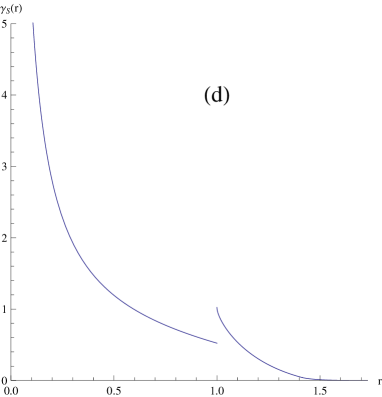
In deriving equation (32) it was implicitly assumed that the given surface intersects its translated image along a curve. In the reality it can happen that for some translation directions the intersection be a surface subset. An illustration of this phenomenon is shown in Figure 8 that refers to a cubic surface of area . The red polygon, shown in Fig. 8a, is the intersection set of the outset cubic surface with its image resulting by the translation of the cubic surface by . This vector is such that its tip point does not lie over one of the cube faces. The case where fully lies over one of the cube faces leads to an intersection set that is formed by two surfaces that respectively have their borders equal to the red thick continuous and broken rectangles shown in Fig.8b. When theonly tip of spans one of the cube faces the intersection set is again a surface whose boundary is given by the red rectangle shown in Fig. 8c. To get the CF of the cubic surface it is necessary to evaluate integral (21) imposing the aforesaid constraints on . This task was explicitly carried out as detailed in the deposited part of this paper. Here one simply reports the surface CF expressions relevant to the geometrical configurations illustrated in first three panels of Fig. 8.
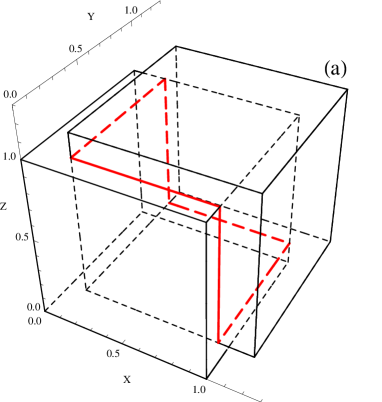
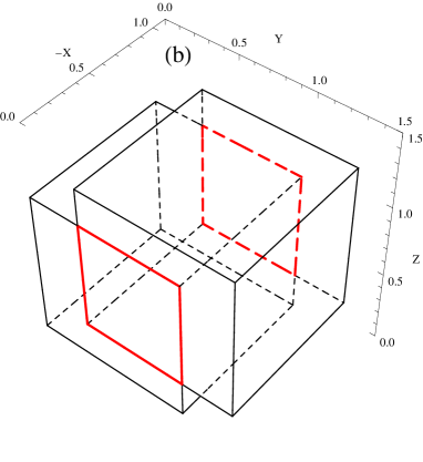
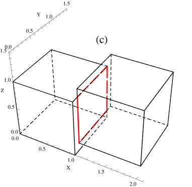
They respectively read
| (110) |
| (111) |
and
| (112) |
Thus, the CF function of a cubic surface is the sum of equations (110) , (111) and (112). Its first moment is equal to , as required by equation (30) while its plot is shown in panel (d) of Fig. 8 for the case . The discontinuity, present at , arises from the opposite faces that are parallel at distance .
Appendix C: small distance behavior of the curve CF
In order to prove equation (60) one proceeds by expanding the parametric equation of the curve around which is the curvilinear coordinate of the point taken as the origin of the Cartesian frame. The expansion up to terms reads
| (113) |
One straightforwardly verifies that vectors , and , obtained by applying definitions (46) to (113) are mutually orthogonal unit vectors up to terms . The condition determines the curvilinear abscissa of the points that are at distance from the origin. As , the equation is easily solved by iteration, putting as first step. The solutions are
| (114) |
Consider the positive solution. One finds that and . In this way, by equation (57), one obtains
| (115) |
The result for the negative solution is the same. In this way result (60) is immediately obtained by (59).
Acknowledgments
We gratefully thank Dr. Wilfried Gille for his critical reading of the ms and for the suggestion of investigating the moments of the curve and the surface CFs.
References
-
Avdeev, M. V., Aksenov, V. L., Gazová, Z., Almásy, L., Petrenko, V. I., Gojzewski, H., Feoktystov, A. V., Siposova, K., Antosova, A., Timko M. & Kopcansky, P. (2013). J. Appl. Cryst. 46, 224-233.
-
Ciccariello, S. (1984). J. Appl. Phys. 56, 162-167.
-
Ciccariello, S. (1989). Acta Cryst. A 45, 86-99.
-
Ciccariello, S. (1991). Phys. Rev. A44, 2975-2983.
-
Ciccariello, S. (1995). J. Math. Phys. 36, 219-246.
-
Ciccariello, S. (2009). J. Math. Phys. 50, 103527/20.
-
Ciccariello, S. (2010). J. Appl. Cryst. 43, 1377-1384.
-
Ciccariello, S. (2014). J. Appl. Cryst. 47, 1866-1881.
-
Ciccariello, S. & Benedetti, A. (1982). Phys. Rev. B26, 6384-6389.
-
Ciccariello, S. & Riello, P. (2007). J. Appl. Cryst. 40, 282-289.
-
Ciccariello, S. & Sobry, R. (1995). Acta Cryst. A 51, 60-69.
-
Ciccariello, S., Cocco, G., Benedetti, A. & Enzo, S. (1981). Phys. Rev. B23, 6474-6485.
-
Debye, P., Anderson, H.R. & Brumberger, H. (1957). J. Appl. Phys. 20, 679-683.
-
Fedorova, I.S. & Emelyanov, V.B. (1977). J. Colloid Interface Sci. 59, 106-112.
-
Feigin, L.A. & Svergun, D.I. (1987). Structure Analysis by Small-Angle X-Ray and Neutron Scattering, New York: Plenum Press.
-
Gille, W. (1999). J. Appl. Cryst. 32, 1100-1104.
-
Gille, W. (2014). Particle and Particle Systems characterization , London: CRC.
-
Goodisman, J. & Brumberger, H. (1971). J. Appl. Cryst. 4, 347-351.
-
Glatter, O. (1982). Small-Angle X-Ray Scattering. Edts Glatter, O. & Kratky, O., London: Academic Press.
-
Gradshteyn, I.S. & Ryzhik, I.M. (1980). Tables of Integrals, Series and Products, New York: Academic Press.
-
Guinier, A. & Fournet, G. (1955). Small-Angle Scattering of X-rays. New York: John Wiley.
-
Kirste, R.G. & Porod, G. (1962). Kolloid Z. 184, 1-6.
-
Kirste, R.G. & Oberthür, R.C. (1982). Small-Angle X-Ray Scattering. Edt.s Glatter, O. & Kratky, O., London: Academic Press
-
Kostorz, G. (1979). Neutron Scattering, Ed. Kostorz, G., London: Academic Press, pp 227-289.
-
Melnichenko, Y.B. & Ciccariello, S. (2012). J. Phys. Chem. C 116, 24661-24671.
-
Méring, J. & Tchoubar, D. (1968). J. Appl. Cryst. 1, 153-65.
-
Peterlin, A. (1965). Makromol. Chem. 87, 152-160.
-
Porod, G. (1951). Kolloid Z. 124, 83-114.
-
Porod, G. (1967). Small-Angle X-Ray Scattering. Proceedings of the Syracuse Conference, Ed. H. Brumberger, 1-8, New York: Gordon & Breach.
-
Porod, G. (1982). Small-Angle X-Ray Scattering. Edt.s Glatter, O. & Kratky, O., London: Academic Press.
-
Smirnov, V.I. (1970). Cours de Mathématiques Supérieures, Moscow: Mir, Vol. II, Chap. V.1.
-
Teubner, M. (1990). J. Chem. Phys. 92, 4501-4507.
-
Wu, H. & Schmidt, P. W. (1974). J. Appl. Cryst. 7, 131-146.