Numerical study of the stability of the Peregrine breather

Abstract.

The Peregrine breather is widely discussed as a model for rogue waves in deep water. We present here a detailed numerical study of perturbations of the Peregrine breather as a solution to the nonlinear Schrödinger (NLS) equations. We first address the modulational instability of the constant modulus solution to NLS. Then we study numerically localized and nonlocalized perturbations of the Peregrine breather in the linear and fully nonlinear setting. It is shown that the solution is unstable against all considered perturbations.

1. Introduction

The importance of rogue waves needs hardly be stressed, and the attempts in the mathematical modelling of these phenomena have been intensified in recent years. Since the governing equations for hydrodynamics are similar to the ones from nonlinear optics, also optical rogue waves have been experimentally and analytically studied recently, see [15] for a review. In deep water and nonlinear optics the focusing nonlinear Schrödinger (NLS) equation

(1) $$iu_{t}+u_{xx}+2|u|^{2}u=0.$$

for a complex $u(x,t)$ describing the modulation of a carrier wave is an important model equation. This is because its solutions show nonlinear focusing and a modulation instability, i.e., self-induced amplitude modulation of a continuous wave propagating in a nonlinear medium, with subsequent generation of localized structures. For a discussion of NLS in the context of rogue waves see for instance [20] and references therein. It is fair to say that no complete understanding of rogue waves has yet been reached. For complementary approaches see for instance [5, 6].

Remarkably the NLS equation has solutions called breathers that show the features of the popular definition of rogue waves as ‘waves that appear from nowhere and disappear without a trace’, see for instance [1]. The most popular nonperiodic breather solution in this context is the Peregrine breather [21]

(2) $$u_{Per}=\left(1-\frac{4(1+4it)}{1+4x^{2}+16t^{2}}\right)e^{2it},$$

which is an exact solution of the focusing NLS equation. It has the property to have constant modulus for $|t|\to\infty$, thus appearing from nowhere and disappearing after some time, and for $|x|\to\infty$. The maximum of $|u|$ is reached for $x=t=0$ and is three times the asymptotic value. Exact NLS solutions describing multiple breathers are given in [12], for an alternative approach to generate breather solutions see [16]. It is reported that the Peregrine solution has been recently observed experimentally in hydrodynamics [8, 9], in plasma physics [2] and in nonlinear optics [17].

For a solution to be of practical relevance in the context of rogue waves, it must be sufficiently robust to be observable in a realistic environment where the initial conditions are never exactly given by the solution (2), but are at best random perturbations thereof. This means one has to study perturbations of Peregrine initial data and to investigate whether the resulting perturbed solution to the NLS equation is in some sense close to (2). This is a difficult task mathematically even in a linearized setting, i.e., for small amplitude perturbations, since the background solution is not constant in time. The question of nonlinear stability is even more out of reach. Thus with the currently available techniques, one has to address this question numerically. For periodic breathers, this has been recently done in [7]. An experimental study of the stability of the Peregrine breather appearing in hydrodynamical experiments against wind was described in [10].

It is the goal of the present paper to present a detailed numerical study of the stability of the Peregrine solution. We consider first small perturbations, e.g., the evolution of initial data of the form $u(x,0)=u_{Per}(x,0)+v(x)$ with $||v(x)||_{\infty}\ll 1$ according to the NLS equation (1). Of special interest are localized perturbations $v(x)$ in the Schwartz space of smooth rapidly decreasing functions $\mathbb{S}(\mathbb{R})$. The second kind of perturbation to be studied is of the form $u_{0}(x)=\sigma u_{Per}(x,t_{0})$ with $\sigma\sim 1$. This means we will study both rapidly decreasing and non decreasing perturbations of the Peregrine breather.

The paper is organized as follows: in section 2 we collect some mathematical preliminaries needed for the following sections. In section 3 we study the absolute instability of the asymptotic state of the Peregrine solution, i.e., of a solution with constant modulus. In section 4, we present a numerical study of the linearized (on the Peregrine background) NLS equation for localized and nonlocalized perturbations. In section 5, localized and nonlocalized perturbations of the Peregrine breather are studied for the full NLS equation to explore the nonlinear stability of the breather. We add some concluding remarks in section 6.

2. Preliminaries

In this section we collect some mathematical information on the NLS equation and linearizations on the background of the Peregrine breather needed for the ensuing stability study. We also briefly review the numerical techniques to be applied in the following.

2.1. NLS and linearized equation

It was shown by Zakharov and Shabat [23] that the NLS equation is completely integrable, i.e., it has an infinite number of conserved quantities the most prominent of which being the mass, the square of the $L^{2}$ norm of $u$ and the energy. Since we want to discuss in this note solutions not decaying to 0 at infinity but with $\lim_{|x|\to\infty}|u|=\kappa>0$ (i.e., solutions which are not in $L^{2}$), we consider instead the quantity

(3) $$\mathcal{E}=\frac{1}{2}\int_{R}\left(|u_{x}|^{2}-|u|^{2}(|u|^{2}-\kappa)\right)dx,$$

which is a combination of mass and energy. The complete integrability of the NLS equation is the reason why many explicit solutions as solitons or breathers are known.

The NLS equation has also some conformal symmetry which implies that with $u(x,t)$ also

(4) $$u^{\sigma}(x,t)=\sigma u(\sigma x,\sigma^{2}t),\quad\sigma\in\mathbb{R},$$

is a solution of NLS. This mean that asymptotically nonvanishing NLS solutions could be always transformed by a suitable choice of $\sigma$ in (4) to have modulus 1 at infinity.

We first study linearizations of the NLS equation (1) of the form $u=u_{Per}+v$ which leads in lowest order of $v$ to the equation

(5) $$iv_{t}+v_{xx}+4|u_{Per}|^{2}v+2u_{Per}^{2}\bar{v}=0.$$

It is straight forward to check that this equation has the conserved quantity (this is a consequence of the conservation of the $L^{2}$ norm for solutions to the NLS equation)

(6) $$M=\int_{\mathbb{R}}(u_{Per}\bar{v}+\bar{u}_{Per}v)dx.$$

Note that there are different ways to linearize the NLS equation (1). An alternative form is to write $u=u_{Per}(1+\tilde{v})$ which implies

(7) $$i\tilde{v}_{t}+\tilde{v}_{xx}+2(\ln u_{Per})_{x}\tilde{v}_{x}+4|u_{Per}|^{2}\Re\tilde{v}=0,$$

for NLS (1) in lowest order of $\tilde{v}$. The disadvantage of equation (7) from a numerical point of view is that it is singular at the zeros of the Peregrine solution for $t=0$. Even for finite small $t$, the fact that one is close to a singularity is numerically problematic. Therefore we study in this note for linearizations numerically only equation (5). However, equation (7) is convenient for analytical approaches, see the following section.

2.2. Numerical methods

We use in this paper spectral methods in $x$, i.e., methods which show for a smooth solution an exponential decrease of the numerical error with the number of collocation points. For the time integration, we use fourth order methods. The accuracy of the numerical computation is controlled via conserved quantities. Because of unavoidable numerical errors, these are in an actual computation not exactly conserved, but can be used as a valid indicator of the reached precision: as shown for instance in [19], they tend to overestimate the numerical accuracy by 1-2 orders of magnitude.

For rapidly decreasing $v(x,\cdot)$ in (5), we use a Fourier spectral method for the spatial dependence and an exponential time differencing (ETD) scheme due to Cox and Matthews [11] for the time integration. The latter scheme uses an exact integration of the linearized equation in Fourier space. The modulus of the Fourier coefficients in the spatial coordinate indicates the spatial resolution since it is known that they decrease exponentially for analytic functions. In all studied examples in this paper, they decrease to machine precision (here $\approx 10^{-15}$) during the whole computation which indicates that the solution is always fully resolved spatially.

For nonlocalized perturbations of the Peregrine solution (2) in the full NLS equation (1), Fourier methods are not appropriate. The algebraic decrease of the solution for $|x|\to\infty$ makes it difficult to periodically continue the solution as an analytic function within the finite numerical precision as can be done with Schwartz functions. To obtain spectral convergence also in this context, a novel numerical approach has been presented in [4]: the real line is divided into several domains each of which is mapped to $[-1,1]$ with a Möbius transformation. Near infinity we use $1/x$ as a local coordinate which allows to cover the whole real line with this approach. Note that we use in contrast to [4] four domains here among which just one compactified one (with $1/x$ as a coordinate). This is due to the symmetric (in $x$) problem studied here in contrast to [4]. On each domain we use polynomial interpolation to obtain on each interval a spectral method. Imposing at the domain boundaries the conditions that the solution be $C^{1}$ there implies with the analytic properties of the NLS equation (which is a second order PDE in $x$) that we obtain a spectral method on the whole real line. For the time integration, we use again a fourth order method.

For details the reader is referred to [19] and [4] and references given therein. Note that the numerical approaches are completely independent for the localized perturbations in the linear case and the nonlinear case. Therefore we compare the results in these cases showing that they are qualitatively similar until the nonlinearity dominates in the latter case. This gives further evidence for the validity of the presented results.

3. Absolute instability of the asymptotic state

A problem in the stability study of the Peregrine solution is the fact that it depends both on $x$ and $t$. Therefore, for the analytical study in this section, we focus on the stability of the asymptotic state for $x\to\infty$ when $u_{Per}\to e^{2it}$. Instabilities of asymptotic states typically induce instabilities of the corresponding exact solutions, however we do not attempt to give a rigorous proof of this fact for the Peregrine solution.

The asymptotic state $e^{2it}$ of the Peregrine solution $u_{Per}$ has constant modulus, so that for our analysis it is more convenient to use the linearized equation (7). For complex perturbations of the form $\tilde{v}=\alpha+i\beta$ we obtain the system

(8) $$\alpha_{t}+\beta_{xx}=0,\quad\beta_{t}-\alpha_{xx}-4\alpha=0,$$

which has constant coefficients. Our purpose is to study the spectral properties of the matrix-operator defined through

$$\mathcal{L}(\alpha,\beta)=(-\beta_{xx},\alpha_{xx}+4\alpha),$$

and acting in $L^{2}(\mathbb{R})\times L^{2}(\mathbb{R})$. This function space corresponds to a choice of localized perturbations, but the instability results below also hold for the larger class of nonlocalized perturbations. We compute the spectrum, which coincides with the essential spectrum, of the operator $\mathcal{L}$, and then the absolute spectrum. Absolute spectra, which are always located to the left of essential spectra in the complex plane, allow to distinguish between absolute instabilities, when perturbations grow in time at each point of the domain, and convective instabilities, when though overall norms grow in time, perturbations locally decay: growing perturbations are convected away towards infinity (e.g., see [22] and the references therein).

Since the operator $\mathcal{L}$ has constant coefficients, these spectra can be determined from the dispersion relation

(9) $$\mathcal{D}(\lambda,\nu)=\lambda^{2}+\nu^{2}(\nu^{2}+4),,$$

obtained by looking for solutions of (8) of the form $(\alpha,\beta)(x,t)=e^{\lambda t+\nu x}(a,b)$, for complex numbers $\lambda,\nu$ and $a,b$. First, the essential spectrum, which coincides with the full spectrum of the operator $\mathcal{L}$ in this case, is the set

$$\sigma=\{\lambda\in\mathbb{C}\;;\;\mathcal{D}(\lambda,ik)=0,\mbox{ for some }k\in\mathbb{R}\}.$$

Then

$$\sigma=\{\lambda\in\mathbb{C}\;;\;\lambda^{2}=k^{2}(4-k^{2}),\mbox{ for some }k\in\mathbb{R}\},$$

implying $\sigma=i\mathbb{R}\cup[-2,2]$. In particular, the set $\sigma$ contains values in the open right hand complex plane showing that the asymptotic state of the Peregrine solution is (essentially) spectrally stable.

Next, the absolute spectrum is found by looking at the relative location in the complex plane of the solutions $\nu\in\mathbb{C}$ of the dispersion relation $\mathcal{D}(\lambda,\nu)=0$ for $\lambda\in\mathbb{C}$ [22]. More precisely, for complex numbers $\lambda$ with large real part, the dispersion relation (9) has two roots $\nu_{1}^{+}(\lambda)$, $\nu_{2}^{+}(\lambda)$ with positive real parts, $\mathrm{Re}\,\nu_{1}^{+}(\lambda)\geq\mathrm{Re}\,\nu_{2}^{+}(\lambda)>0$, and two roots $\nu_{1}^{-}(\lambda)$, $\nu_{2}^{-}(\lambda)$ with negative real parts, $\mathrm{Re}\,\nu_{1}^{-}(\lambda)\leq\mathrm{Re}\,\nu_{2}^{-}(\lambda)<0$. Then in this case, the absolute spectrum of the operator $\mathcal{L}$ is simply defined by

$$\sigma_{abs}=\{\lambda\in\mathbb{C}\;;\;\mathrm{Re}\,\nu_{2}^{+}(\lambda)=\mathrm{Re}\,\nu_{2}^{-}(\lambda)\}.$$

The essential instability found above is absolute if there exists $\lambda\in\sigma_{abs}$ with $\mathrm{Re}\,\lambda>0$. Since the dispersion relation is invariant under the change $\nu\mapsto-\nu$, we have that $\nu_{j}^{-}(\lambda)=-\nu_{j}^{+}(\lambda)$, for $j=1,2$, implying that $\mathrm{Re}\,\nu_{2}^{+}(\lambda)=\mathrm{Re}\,\nu_{2}^{-}(\lambda)=0$ when $\lambda\in\sigma_{abs}$. As a consequence, the absolute spectrum coincides with the essential spectrum here, $\sigma_{abs}=\sigma=i\mathbb{R}\cup[-2,2]$, showing that the instability of the asymptotic state of the Peregrine solution is absolute.

4. Numerical simulations for the linearized equation

In this section, we study perturbations of the Peregrine breather in the linearized regime. This means we study initial value problems for the linear equation (5) both for rapidly decreasing initial data and for data proportional to the Peregrine solution. We find in both cases that the solution grows strongly in time which confirms the absolute instability discussed in the previous section. Because of the time dependent background leading to a nonautonomous equation (5), the growth in time is not exponential.

4.1. Rapidly decreasing perturbations

For the numerical experiments, we concentrate on equation (5) and the initial data $v=0.1e^{-x^{2}}$. Since these data are rapidly decreasing, we use as discussed in section 2 a Fourier spectral method for the spatial dependence. The computation is carried out with $N=2^{14}$ Fourier modes and $N_{t}=10^{4}$ time steps. The modulus of the Fourier coefficients decreases to machine precision during the whole computation which indicates that the solution is fully resolved spatially. The relative change of the conserved quantity (6) during the computation is of the order of $10^{-10}$ which indicates that the solution shown in Fig. 1 should be accurate at least to the order of $10^{-8}$.

Figure 1. Numerical solution to the linearized NLS equation (5) for the initial data $v=0.1e^{-x^{2}}$

.

The maximum of the solution is visibly quickly growing and becomes larger than the modulus of the Peregrine solution itself which indicates that the linearized regime is left, in other words that the solution is unstable. Moreover the initial peak is also being dispersed to $\pm\infty$ as can be seen in Fig. 1.

4.2. Nonlocalized perturbations

We consider nonlocalized data proportional to the breather. We use the same numerical approach as for the fully nonlinear equation and the same parameters as detailed there. For the initial data $v(x,0)=0.1u_{Per}(x,0)$, we get the solution shown in Fig. 2. As for the localized perturbations in Fig. 1, the solution is clearly unstable and quickly leaves the linearized regime.

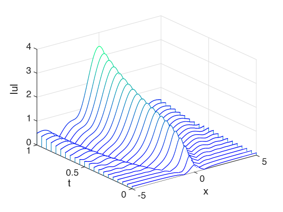
Figure 2. Numerical solution to the linearized NLS equation (5) for the initial data $v=0.1u_{Per}$

.

5. Nonlinear Stability

In this section, we will study perturbations of the Peregrine breather for the full NLS equation (1). We again consider localized and nonlocalized perturbations to the Peregrine breather as in the linearized case and find that the breather is unstable against all perturbations. This also applies if the solution is perturbed at an earlier time: the resulting NLS solution for these perturbed initial data will not be close to the Peregrine breather at $t=0$ or later times.

The numerical approach uses four domains for $x$: domain I with $x\in[-20,-5]$, domain II with $x\in[-5,5]$, domain III with $x\in[5,20]$; the compactified domain IV is defined via $-1/20<1/x<1/20$. Thus we solve the NLS equation on the whole real line. In the respective domains, we use $N_{I}=N_{III}=200$, $N_{II}=300$ and $N_{IV}=100$ Chebyshev polynomials. We always take the time step $\Delta_{t}=10^{-3}$. The numerical accuracy is controlled via the conserved quantity $\mathcal{E}$ in (3) in the form of the relative quantity

(10) $$\Delta_{E}=1-\frac{\mathcal{E}(t)}{\mathcal{E}(t_{0})},$$

(because of numerical errors the computed $\mathcal{E}$ will be time dependent).

5.1. Rapidly decreasing perturbations

We first study as in the previous section initial data of the form $u(x,0)=u_{Per}(x,0)+0.1\exp(-x^{2})$. The resulting solution can be seen in Fig. 3 where the initial hump appears to be dispersed away to infinity, but in a significantly different way than the Peregrine breather.

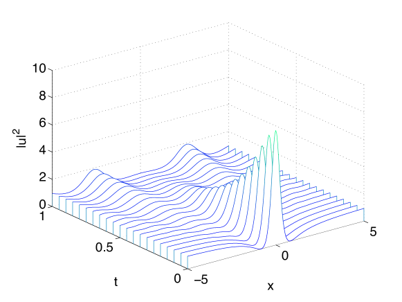
Figure 3. Solution to the NLS equation for the initial data $u_{Per}(x,0)+0.1\exp(-x^{2})$ in dependence of time.

This is even more obvious in the left figure of Fig. 4 where the solution at the last computed time is shown together with the Peregrine solution (2) at the same time. Clearly the Peregrine breather is unstable against this type of perturbations, and the perturbed solution does not stay close to the exact solution. Note that the solution is even at the last computed time well resolved spatially as can be seen in the right figure of Fig. 4, where the Chebyshev coefficients at the last computed time are shown. Since the initial data are symmetric with respect to the transformation $x\to-x$ and since the Schrödinger equation preserves parity, the Chebyshev coefficients in zone I and III are identical (therefore the coefficients in zone III are not shown), and half of the coefficients in zone II and IV vanish with numerical precision. The coefficients in zone IV still decrease to $10^{-4}$. As discussed in [4], the slow decrease of the Chebyshev coefficients is due to the oscillations with a slowly decreasing amplitude for $|x|\to\infty$. The conserved quantity (10) is $\Delta_{E}\sim 8.8*10^{-3}$. This implies together with the resolution in coefficient space shown in Fig. 4 that the solution is computed to at least plotting accuracy.

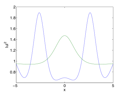
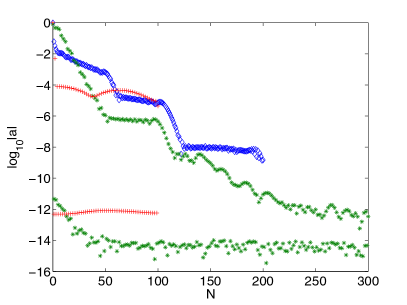
Figure 4. Solution to the NLS equation shown in Fig. 3 at $t=1$ in blue and the Peregrine breather (2) for $t=1$ in green on the left, and the corresponding Chebyshev coefficients for the numerical solution on the right (in blue for domain I, green for domain II and red for domain III).

In Fig. 5 we show the difference between the numerical solution $u$ in Fig. 3 and the Peregrine solution. This corresponds to the function $v$ in the linearized case (5), and Fig. 5 thus has to be compared to Fig. 1. It is interesting to see that both figures are qualitatively similar, but that the nonlinearity has the effect to delimit the growing of $|u-u_{Per}|$ for later times and to disperse the solution more efficiently.

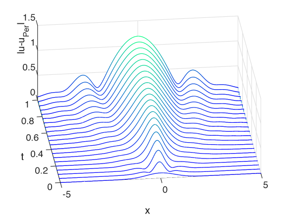
Figure 5. Difference between the solution to the NLS equation shown in Fig. 3 and the Peregrine breather (2).

It is an interesting question whether a perturbation of the breather at an earlier time still allows to observe a Peregrine type behavior at $t\sim 0$ at least in a qualitative sense. To answer this question, we consider as initial data $u(x,-1)=u_{Per}(x,-1)+0.1\exp(-x^{2})$ in Fig. 6. It can be recognized that the solution grows to a similar maximal value as the Peregrine solution, but reaches it at an earlier time. The focusing effect of the focusing NLS equation is clearly visible, but it does not force the solution towards the Peregrine breather.

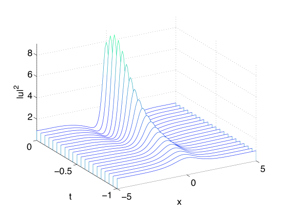
Figure 6. Solution to the NLS equation for the initial data $u(x,-1)=u_{Per}(x,-1)+0.1\exp(-x^{2})$ in dependence of time.

In Fig. 7, it can be seen that the solution at the last recorded time is clearly different from the Peregrine solution 2 which again confirms that the solution is unstable. The Chebyshev coefficients at the last recorded time can be seen in Fig. 7 on the right showing that the solution is well resolved.

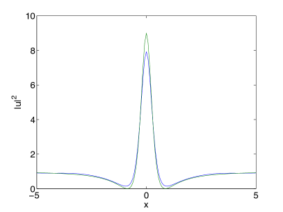
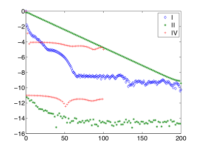
Figure 7. Solution to the NLS equation shown in Fig. 6 at $t=0$ in blue and the Peregrine breather (2) for $t=0$ in green on the left, and the corresponding Chebyshev coefficients for the numerical solution on the right (in blue for domain I, green for domain II and red for domain III).

5.2. Nonlocalized perturbations

In this subsection we study nonlocalized perturbations of the breather of the form $u(x,t_{0})=\sigma u_{Per}(x,t_{0})$, where $\sigma\sim 1$. The parameters for the numerical computation are as in the previous subsection.

In Fig. 8 we show the solution for the initial data $u(x,0)=1.1u_{Per}(x,0)$ in dependence of time. It can be seen that the solution keeps growing despite being initially already above the global maximum of the Peregrine solution before decreasing, but in contrast to the latter not monotonically. Instead it grows again before being eventually dispersed. Note that the quantity $\mathcal{E}$ in (3) is positive in this case.

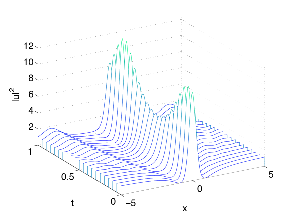
Figure 8. Solution to the NLS equation for the initial data $u(x,0)=1.1u_{Per}(x,0)$ in dependence of time.

It is obvious, see also the left figure in Fig. 9, that the solution at the final recorded time is not close to the Peregrine solution at the same time. Clearly the Peregrine solution is also nonlinearly unstable against unbounded perturbations proportional to the solution itself. The right figure in Fig. 9 shows that the solution is again well resolved spatially even at the final time of computation. For the quantity (10) we have $\Delta_{E}<8.15*10^{-4}$ during the whole computation.

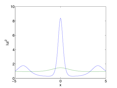
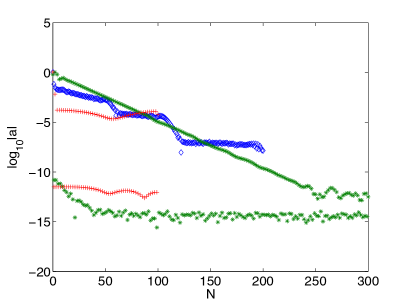
Figure 9. Solution to the NLS equation shown in Fig. 8 at $t=1$ in blue and the Peregrine breather (2) for $t=1$ in green on the left, and the corresponding Chebyshev coefficients for the numerical solution on the right (in blue for domain I, green for domain II and red for domain III).

In Fig. 10 we show the difference of the numerical solution in Fig. 8 and the Peregrine breather in dependence of $t$. This can be compared to the solution of the linearized equation (5) in Fig. 2. It can be seen that the solution to the linearized equation (5) grows continually, whereas the solution to the full NLS equation reaches a maximum and decreases then. Note however the qualitative similarity at earlier times.

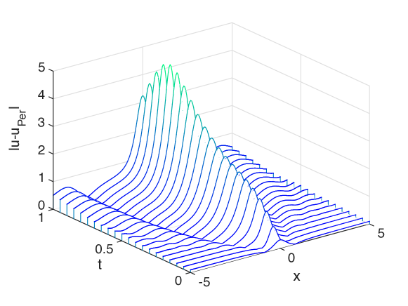
Figure 10. Difference of the solution to the NLS equation shown in Fig. 8 and the Peregrine breather (2).

A similar perturbation as in Fig. 8 but of positive $\mathcal{E}$ is considered in Fig. 11 where the initial data are $u(x,0)=0.9u_{Per}(x,0)$. Here the solution never reaches the maximum of the Peregrine solution. Instead it decreases in modulus with time, but also not as the latter solution, but by radiating the mass towards infinity in the form of dispersive oscillations.

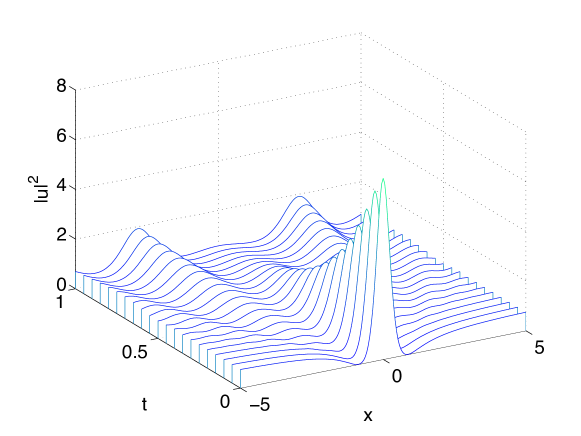
Figure 11. Solution to the NLS equation for the initial data $u(x,0)=0.9u_{Per}(x,0)$ in dependence of time.

Fig. 12 shows that the solution is again in no sense close to the Peregrine solution (2). The Chebyshev coefficients in the same figure decrease again to the order of $10^{-4}$. During the whole computation we have $\Delta_{E}<4.43*10^{-5}$.

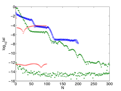
Figure 12. Solution to the NLS equation shown in Fig. 11 at $t=1$ in blue and the Peregrine breather (2) for $t=1$ in green on the left, and the corresponding Chebyshev coefficients for the numerical solution on the right (in blue for domain I, green for domain II and red for domain III).

In Fig. 13 we show the difference of the solution in Fig. 11 and the Peregrine breather which can be compared to the solution of the linearized equation (5) in Fig. 2. Note that the solution of the linearized equation (5) is identical for the cases corresponding to Fig. 8 and Fig. 11. Clearly this is not the case for the solutions to the full NLS equation, but there is good agreement for early times. For larger times, the difference in Fig. 13 grows considerably more slowly than the solution in Fig. 2.

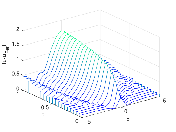
Figure 13. Difference of the solution to the NLS equation in Fig. 11 and the Peregrine breather.

As in the previous subsection, we also address the question whether perturbations of the above kind at an earlier time still allow to qualitatively observe characteristic features of the Peregrine breather (2) at later times. In Fig. 14 we consider the solution for initial data of the form $u(x,-1)=1.1u_{Per}(x,-1)$. In this case $\mathcal{E}$ is again positive, and a higher maximum is reached at an earlier time than for the Peregrine breather, though the solution is qualitatively of a similar form. However, the solution is dispersed away to infinity in a completely different manner than for the Peregrine breather.

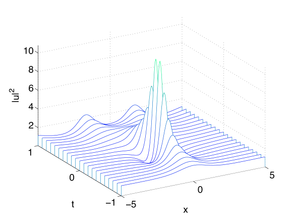
Figure 14. Solution to the NLS equation for the initial data $u(x,-1)=1.1u_{Per}(x,-1)$ in dependence of time.

In Fig. 15 it is, however, obvious that the solution at the final recorded time is not close to the Peregrine breather. The Chebyshev coefficients in the same figure decrease to $10^{-5}$. During the whole computation we have $\Delta_{E}<2.5*10^{-3}$.

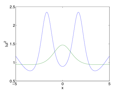
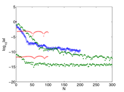
Figure 15. Solution to the NLS equation shown in Fig. 14 at $t=1$ in blue and the Peregrine breather (2) for $t=1$ in green on the left, and the corresponding Chebyshev coefficients for the numerical solution on the right (in blue for domain I, green for domain II and red for domain III).

For the initial data $u(x,-1)=0.9u_{Per}(x,-1)$, i.e., a perturbation of negative $\mathcal{E}$ in (3), the solution is shown in Fig. 16. It can be seen that the solution does not reach the maximum of the Peregrine breather.

Figure 16. Solution to the NLS equation for the initial data $u(x,-1)=0.9u_{Per}(x,-1)$ in dependence of time.

Again the solution is not close to the Peregrine breather at the final recorded time as can be seen in Fig. 17. The solution is well resolved in the space of Chebyshev coefficients as can be seen in the same figure. During the whole computation we have $\Delta_{E}<9.05*10^{-4}$.

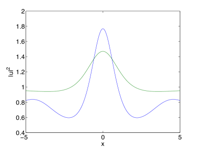
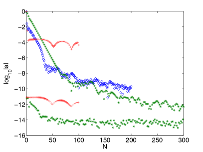
Figure 17. Solution to the NLS equation shown in Fig. 16 at $t=1$ in blue and the Peregrine breather (2) for $t=1$ in green on the left, and the corresponding Chebyshev coefficients for the numerical solution on the right (in blue for domain I, green for domain II and red for domain III).

6. Conclusion

The results of the previous section indicate that solutions to the focusing NLS equation are not stable if they do not vanish for $|x|\to\infty$, and that this instability is absolute. This appears to be the case whether the perturbation is localized or not. On the other hand the focusing effect of the NLS equation is of course always present. In fact it seems that the Peregrine breather is not stable, but appears in an asymptotic sense explained below locally in strongly focused peaks. Note that the behavior shown above is actually observed in experiments in nonlinear optics for initial data close to the Peregrine breather [18].

If one considers initial data with a support on scales of order $1/\epsilon$ and studies the corresponding NLS solution on time scales of order $1/\epsilon$, this can be conveniently done by the coordinate change $x\to\epsilon x$, $t\to\epsilon t$ which leads for (1) to

(11) $$i\epsilon u_{t}+\epsilon^{2}u_{xx}+2|u|^{2}u=0.$$

It is well known that solutions to the NLS equation in the semiclassical limit $\epsilon\ll 1$ for analytic initial data in $L^{2}$ with a single maximum become strongly peaked at $t\sim t_{c}$ where $t_{c}$ is the critical time where the solution to the semiclassical system (the system following from (11) by formally letting $\epsilon\to 0$) for the same initial data develops a cusp. An example for Gaussian initial data is shown in Fig. 18.

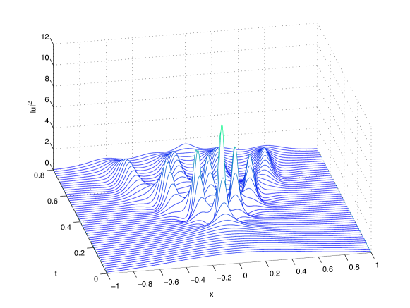
Figure 18. Solution to the NLS equation (11) with $\epsilon=0.1$ for the initial data $u_{0}=\exp(-x^{2})$.

In [13, 14] it was conjectured that the local (in the vicinity of the cusp) behavior of the NLS solution for $t\sim t_{c}$ is asymptotically for $\epsilon\to 0$ given by the tritronquée solution to the Painlevé I equation. A partial proof of this conjecture was given in [3]. In [3] it was also shown that the Peregrine breather appears in the asymptotic (local) description of the peak of the NLS solution in the semiclassical limit and is in this sense universal.

References

- [1] N. Akhmediev, A. Ankiewicz, and M. Taki, Waves that appear from nowhere and disappear without a trace, Phys. Lett. A, 373, 675–678 (2009).
- [2] H. Bailung, S. K. Sharma, and Y. Nakamura, Observation of Peregrine solitons in a multicomponent plasma with negative ions, Phys. Rev. Lett. 107, 255005 (2011).
- [3] M. Bertola and A. Tovbis, Universality for the focusing nonlinear Schrödinger equation at the gradient catastrophe point: rational breathers and poles of the Tritronquée solution to Painlevé-I. Comm. Pure Appl. Math., 66, no. 5, 678–752 (2013).
- [4] M. Birem and C. Klein, Multidomain spectral method for Schrödinger equations, preprint arxiv.org/abs/1410.3718.
- [5] J. Bona and J.-C. Saut, Dispersive Blow-Up II. Schrödinger-Type Equations, Optical and Oceanic Rogue Waves, Chinese Annals of Math. Series B, 31, (6), (2010), 793-810.
- [6] J.L. Bona, G. Ponce, J.-C. Saut, C. Sparber, Dispersive blow-up for nonlinear Schr dinger equations revisited, JMPA, 102, 782–811 (2014).
- [7] A. Calini and C.M. Schober, Numerical investigation of stability of breather-type solutions of the nonlinear Schrödinger equation, Nat. Hazards Earth Syst. Sci., 14, 1431–1440 (2014).
- [8] A. Chabchoub, N. P. Hoffmann, and N. Akhmediev, Rogue wave observation in a water wave tank, Phys. Rev. Lett., 106, 204502 (2011).
- [9] A. Chabchoub, N. Hoffmann, M. Onorato, and N. Akhmediev, Super rogue waves: observation of a higher-order breather in water waves, Phys. Rev. X 2, 011015 (2012).
- [10] A. Chabchoub, N. Hoffmann, H. Branger, C. Kharif, and N. Akhmediev, Experiments on wind-perturbed rogue wave hydrodynamics using the Peregrine breather model, Physics of Fluids, 25, DOI: 10.1063/1.4824706 (2013).
- [11] S. Cox and P. Matthews, Exponential time differencing for stiff systems, Journal of Computational Physics, 176, 430–455 (2002).
- [12] P. Dubard, P. Gaillard, C. Klein, and V.B. Matveev, On multi-rogue wave solutions of the NLS equation and positon solutions of the KdV equation, Eur. Phys. J. Special Topics, 185, 247–258 (2010).
- [13] B. Dubrovin, T. Grava, and C. Klein, On universality of critical behaviour in the focusing nonlinear Schrödinger equation, elliptic umbilic catastrophe and the tritronquée solution to the Painlevé-I equation, J. Nonl. Sci., 19(1), 57–94 (2009).
- [14] B. Dubrovin, T. Grava, C. Klein, and A. Moro, On critical behaviour in systems of Hamiltonian partial differential equations, J. Nonl. Sci., 25(3), 631–707 (2015).
- [15] J.M. Dudley, F. Dias, M. Erkintalo, and G. Genty, Instabilities, breathers and rogue waves in optics, Nature Photonics 8, 755–764 (2014).
- [16] C. Kalla, Breathers and solitons of generalized nonlinear Schrödinger equations as degenerations of algebro-geometric solutions, J. Phys. A: Math. Theor. 44, DOI:10.1088/1751-8113/44/33/335210 (2011).
- [17] B. Kibler, J. Fatome, C. Finot, G. Millot, F. Dias, G. Genty, N. Akhmediev, and J. M. Dudley, The Peregrine soliton in nonlinear fibre optics, Nat. Phys. 6, 790–795 (2010).
- [18] B. Kibler, private communication.
- [19] C. Klein, Fourth order time-stepping for low dispersion Korteweg-de Vries and nonlinear Schrödinger equation, ETNA, 29, 116–135 (2008).
- [20] A. Osborne, M. Onorato, and M. Serio, The nonlinear dynamics of rogue waves and holes in deep-water gravity wave trains, Phys. Lett. A, 275, 386–393 (2000).
- [21] D.H. Peregrine, Water waves, nonlinear Schrödinger equations and their solutions, J. Austral. Math. Soc. B, 25, 16–43, DOI:10.1017/S0334270000003891 (1983).
- [22] B. Sandstede and A. Scheel, Absolute and convective instabilities of waves on unbounded and large bounded domains, Physica D, 145, 233–277 (2000).
- [23] V.E. Zakharov and A.B. Shabat, Exact theory of two-dimensional self-focusing and one-dimensional selfmodulation of waves in nonlinear media. Sov. Phys. JETP, 34(1), 62–69 (1972); translated from Zh. Eksp. Teor. Fiz. 1, 118–134 (1971).