Keywords: Metadynamics, Umbrella Sampling, Reweighting, Weighted Histogram Analysis, Free energy calculations

Abstract

Metadynamics (MTD) is a very powerful technique to sample high–dimensional free energy landscapes, and due to its self–guiding property, the method has been successful in studying complex reactions and conformational changes. MTD sampling is based on filling the free energy basins by biasing potentials and thus for cases with flat, broad and unbound free energy wells, the computational time to sample them becomes very large. To alleviate this problem, we combine the standard Umbrella Sampling (US) technique with MTD to sample orthogonal collective variables (CVs) in a simultaneous way. Within this scheme, we construct the equilibrium distribution of CVs from biased distributions obtained from independent MTD simulations with umbrella potentials. Reweighting is carried out by a procedure that combines US reweighting and Tiwary–Parrinello MTD reweighting within the Weighted Histogram Analysis Method (WHAM). The approach is ideal for a controlled sampling of a CV in a MTD simulation, making it computationally efficient in sampling flat, broad and unbound free energy surfaces. This technique also allows for a distributed sampling of a high–dimensional free energy surface, further increasing the computational efficiency in sampling. We demonstrate the application of this technique in sampling high–dimensional surface for various chemical reactions using ab initio and QM/MM hybrid molecular dynamics simulations. Further, in order to carry out MTD bias reweighting for computing forward reaction barriers in ab initio or QM/MM simulations, we propose a computationally affordable approach that does not require recrossing trajectories.

1 Introduction

Metadynamics (MTD) is a very powerful tool to sample complex free energy landscapes of complex chemical reactions, phase transitions and conformational changes. [1, 2, 3, 4, 5] MTD is a biased sampling approach where sampling of a selected set of collective variables (CVs) is enhanced by introducing slowly grown smooth history dependent repulsive potentials along the trajectory of CVs. In MTD, the underlying potential energy of a system $U(\mathbf{R})$ is modified to $U(\mathbf{R})+V^{\rm b}(\mathbf{s},t)$, where $V^{\rm b}(\mathbf{s},t)$ is the biasing potential applied along the CVs, $\mathbf{s}\equiv\mathbf{s}(\mathbf{R})$, at any instance of the simulation $t$. Typically, $V^{\rm b}(\mathbf{s},t)$ is constructed by the sum of spherical Gaussians deposited over time, as

$$V^{\rm b}(\mathbf{s},t)=\sum_{\tau<t}w_{\tau}\exp\left[-\frac{\left\{\mathbf{s}-\mathbf{s}(\tau)\right\}^{2}}{2(\delta s)^{2}}\right]$$ (1)

Here $w_{\tau}$ and $\delta s$ are the height and the width parameters defining the Gaussian potential added at some time $\tau$. In Well–Tempered MTD (WT–MTD) [6],

$$w_{\tau}=\omega_{0}\tau_{0}\exp\left[-\frac{V^{\rm b}(\mathbf{s},t)}{k_{\rm B}\,\Delta T}\right]$$ (2)

where $\omega_{0}$ is the initial rate of deposition of the bias, $\tau_{0}$ is the time step at which Gaussian potentials are augmented, and $\Delta T$ is a parameter. The advantage of WT–MTD is that a systematic convergence in free energy can be achieved – at the limit $t\rightarrow\infty$, the biasing potential $V^{\rm b}(\mathbf{s},t)$ does not vary much, and

$$\lim_{t\rightarrow\infty}V^{\rm b}(\mathbf{s},t)+f^{\prime}=-\frac{\Delta T}{T+\Delta T}F(\mathbf{s})$$ (3)

where $f^{\prime}$ is a constant. Thus, a converged free energy surface can be constructed as

$$F(\mathbf{s})=-\alpha\lim_{t\rightarrow\infty}V^{\rm b}(\mathbf{s},t)+f$$ (4)

where $\alpha={(T+\Delta T)}/{\Delta T}$ and $f$ is some other constant.[7]

In MTD simulations the total simulation time required to sample a free energy landscape depends exponentially on the number of CVs. Larger the volume of the free energy wells, more is the time required to fill them and to see transitions from one well to the other. Generally, MTD simulations are carried out with 2 or 3 CVs [3]. Although, most of the reactions or structural changes can be sampled using 2 or 3 CVs, one finds several other orthogonal coordinates which have hidden barriers, leading to serious errors in the free energies and poor convergence. Thus inclusion of a few more CVs in sampling would help to accelerate sampling of orthogonal coordinates. In this spirit, MTD has been combined with parallel tempering method [8], and a technique called bias–exchange MTD [9, 10] has been introduced.

An ideal technique to compute free energy along a known reaction path is the Umbrella Sampling (US) method, [11] where a number of time independent harmonic basing potentials are applied to obtain biased probability distribution of CVs. Here the umbrella biasing potential placed at $\mathbf{s}_{h}$,

$$W^{\rm b}_{h}(\mathbf{s})=\frac{1}{2}\kappa_{h}\left(\mathbf{s}-\mathbf{s}_{h}\right)^{2},\enspace h=1,\cdots,M$$ (5)

is used to construct a set of biased probability distributions $\left\{\tilde{P}_{h}(\mathbf{s})\right\}$, from $M$ independent MD simulations with varying biases. Subsequently, $\left\{\tilde{P}_{h}(\mathbf{s})\right\}$ is reweighted to obtain the equilibrium probability distribution $\left\{P_{h}(\mathbf{s})\right\}$ for all the $M$ windows, and are subsequently combined to get the total distribution $P(\mathbf{s})$ through the Weighted Histogram Analysis Method (WHAM). [12, 13] The equilibrium free energy surface is then constructed by

$$F(\mathbf{s})=-\frac{1}{\beta}\ln P(\mathbf{s})+f$$ (6)

where $\beta=(k_{\rm B}T)^{-1}$ and $f$ is some arbitrary constant.

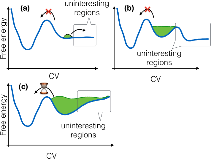
Figure 1: Sketch of free energy surfaces showing three scenarios where traditional MTD simulations fail to sample efficiently. Green color shows the bias added by MTD. For cases (a) and (b), transition from reactant well (broad well at the right side) to the product well (narrow well at the left) would be failed to observe in a standard MTD. In the case of (c), computational overhead would be very high due to the broad reactant basin.

In Figure 1, we sketch some practical limitations of standard MTD simulation in sampling flat potentials. For potentials like those shown in Figure 1a and b, MTD simulations fail to sample transition from reactant to product wells. For the case in Figure 1c, a large number of Gaussian potentials has to be filled in the reactant basin due to its broadness. Chemical reactions in systems such as weakly bound Michaelis complexes in enzymes, weakly bound molecular complexes, and in general A+B type reactions in solutions and gasphase have such free energy topology. Here, MTD spends most of the computational time in filling uninteresting parts of the free energy wells. Partly, these problems can be circumvented by using repulsive wall potentials. However, wall potentials introduce boundary effects and require corrections for the boundary effects. [14, 15] Often it is difficult to scrutinize whether the minimum observed near the boundary is due to the artifact of the wall potential or actual. Also, the coordinate that requires controlled sampling using wall potentials has to be defined as CVs (if they are not part of the CVs already). Alternatively, the coordinate along which the free energy is flat or broad can be efficiently sampled using US since the sampling range of the coordinate can be controlled in US. However, to sample bound orthogonal coordinates with hidden barriers, MTD is ideal because of its self–guiding nature. Thus for an efficient sampling of a high dimensional free energy landscape that has features as in Figure 1 along certain CVs, a combination of US with MTD, where these methods simultaneously sample orthogonal coordinates, is ideal.

Here we report a procedure to carry out such hybrid simulations and to obtain free energy landscape in the full CV space. We name this technique of combining US and MTD as Well–Sliced MTD (WS–MTD). Here $M$ independent MTD simulations are carried out with the bias

$$W^{\rm b}_{h}(\mathbf{s}_{\alpha})+V^{\rm b}_{h}(\mathbf{s}_{\beta},t),\enspace h=1,\cdots,M$$ (7)

to sample the CV space

$$\mathbf{s}\equiv\left(\mathbf{s}_{\alpha},\mathbf{s}_{\beta}\right)\enspace.$$

Here $W^{\rm b}_{h}(\mathbf{s}_{\alpha})$ and $V^{\rm b}_{h}(\mathbf{s}_{\beta},t)$ are given by Equation (5) and Equation (1), respectively. $M$ number of umbrella biases are placed along the $\mathbf{s}_{\alpha}$ coordinates, and for each of these umbrella $h$, we carry out MTD simulation sampling the $\mathbf{s}_{\beta}$ coordinates. Each US+MTD simulation samples a slice of the high–dimensional free energy surface. Subsequently we combine the biased probability distributions from $M$ different US+MTD simulations to construct the total equilibrium distribution and the free energy surface.

Reweighting is not straightforward for MTD, as the biasing potential is time dependent and the sampling weights change with simulation time. Tiana [16] proposed a strategy to obtain ensemble averages from MTD based on a time–dependent reweighting scheme. Employing the convergence property of WT–MTD, a more systematic strategy was reported by Bonomi et al. [17] Laio and co–workers have put forward a different reweighting scheme in the framework of bias–exchange MTD. [10] Recently, a very simple and efficient reweighting scheme was reported by Tiwary and Parrinello [18] based on time dependent weights directly computable from WT–MTD simulations.

Combining US with MTD has been reported first by Frilizola and co–workers [19] where a MTD reweighting proposed by Bonomi et al. [17] was used. US technique has been combined with various sampling techniques; see Ref. [20] for a review and Ref. [21] for a recent example. There were also attempts to do US corrections on the free energy surface obtained from MTD. [22, 23, 24, 25]

Here we combine US and MTD to sample orthogonal coordinates and reconstruct the free energy surface by a combination of Tiwary–Parrinello reweighting scheme and US reweighting within WHAM. First we carefully study the method on a model potential for which the exact free energy barriers are known. Then we extend our study to various problems that are part of the ongoing research in our laboratory, where normal MTD has failed or has poor performance in sampling high dimensional free energy landscape due to the problems shown in Figure 1. In this respect, we first perform ab initio MD simulation of formation of cyclobutene from 1,3–butadiene using WS–MTD and compare its performance with WT–MTD. This serves as an ideal example as its free energy landscape has very broad and deep reactant basin. We then applied WS–MTD to model ligand exchange reactions of Pd complex in aqueous solution where the standard MTD simulations are known to fail. [26] This example shows how controlled sampling of a high dimensional free energy landscape can be achieved by WS–MTD. Finally, we demonstrate the efficiency of WS–MTD in modeling an enzymatic reaction using QM/MM method. Coordination of water molecule to one of the catalytic Zn ions in the active site of New Delhi metallo $\beta$–lactamase 1 (NDM–1) [27] is modeled, for which our earlier attempts using WT–MTD and non–tempered MTD simulations were unsuccessful.

2 Methods and Models

2.1 Reweighting Scheme in WS–MTD

Here we discuss how to obtain the reweighted distribution from WS–MTD simulations. Let us consider a problem where we are interested in computing the free energy surface $F(s_{1},s_{2})$ by sampling the CVs $s_{1}$ and $s_{2}$. Consider that, the coordinate $s_{1}$ is sampled using US, while $s_{2}$ is simultaneously sampled by a one–dimensional WT–MTD. If $M$ umbrella potentials are placed along the $s_{1}$ coordinate, we carry out $M$ independent MTD simulations, each using the Hamiltonian

$$H^{\rm ws}_{h}(\mathbf{R},\mathbf{P})=H^{0}(\mathbf{R},\mathbf{P})+W^{\rm b}_{h}(s_{1})+V^{\rm b}_{h}(s_{2},t)\enspace,\enspace h=1,\cdots,M$$ (8)

with $W^{\rm b}_{h}(s_{1})$ and $V^{\rm b}_{h}(s_{2},t)$ are given by Equation (5), and Equation (1), respectively, and $H^{0}$ is the unbiased Hamiltonian for canonical molecular dynamics. For obtaining $F(s_{1},s_{2})$, we require a strategy to obtain the unbiased probability distribution $P(s_{1},s_{2})$.

When no umbrella bias is present, under the quasi–stationary limit, the time dependent probability distribution from a WT–MTD simulation can be written as,

$$\tilde{P}(\mathbf{R},t)=\frac{\exp\left[-\beta\left\{U(\mathbf{R})+V^{\rm b}(\mathbf{s}(\mathbf{R}),t)\right\}\right]}{\int d\mathbf{R}\,\exp\left[-\beta\left\{U(\mathbf{R})+V^{\rm b}(\mathbf{s}(\mathbf{R}),t)\right\}\right]}$$ (9)

and is related to the unbiased probability distribution $P(\mathbf{R})$ by [17]

$$P(\mathbf{R})=\tilde{P}(\mathbf{R},t)\exp\left[\beta\left\{V^{\rm b}(\mathbf{s}(\mathbf{R}),t)-c(t)\right\}\right]\,$$ (10)

where

$$c(t)=\frac{1}{\beta}\ln\left[\frac{\int d\mathbf{s}\exp[-\beta F(\mathbf{s})]}{\int d\mathbf{s}\exp[-\beta\{F(\mathbf{s})+V^{\rm b}(\mathbf{s},t)\}]}\right]\enspace.$$ (11)

Evaluation of $c(t)$, however, requires a time–independent free energy $F(\mathbf{s})$, which can be computed using the Tiwary–Parrinello time–independent free energy estimator[18] as,

$$F(\mathbf{s})=-\alpha V^{\rm b}(\mathbf{s},t)+\frac{1}{\beta}\ln\int d\mathbf{s}\exp\left[{\alpha\beta V^{\rm b}(\mathbf{s},t)}\right]\enspace,$$ (12)

where the time dependency of the first term cancels with that of the second.

In WS–MTD, we construct the time independent probability distribution $P_{h}^{\rm u}(s_{1},s_{2})$, by reweighting the MTD potential, for each umbrella $h$. On reaching the quasi–stationary limit, the statistical weight at which $s_{2}(\mathbf{R}(t))$ is sampled during MTD (due to MTD bias) is $\exp[-\beta\left\{V_{h}^{\rm b}(s_{2}(\mathbf{R}),t)-c_{h}(t)\right\}]$ (see Equation (10)). Thus,

$$P^{\rm u}_{h}(s_{1}^{\prime},s_{2}^{\prime})=\frac{\int_{t_{\rm min}}^{t_{\rm max}}d\tau\,\exp[\beta\left\{V_{h}^{\rm b}(s_{2}(\tau),\tau)-c_{h}(\tau)\right\}]\enspace\delta(s_{1}(\tau)-s_{1}^{\prime})\enspace\delta(s_{2}(\tau)-s_{2}^{\prime})}{\int_{t_{\rm min}}^{t_{\rm max}}d\tau\,\exp[\beta\left\{V_{h}^{\rm b}(s_{2}(\tau),\tau)-c_{h}(\tau)\right\}]}\enspace.$$ (13)

In practice, for each $h$, we compute the above equation by discrete sum over the MTD trajectory of $\{s_{1}(t),s_{2}(t)\}$. The numerator is computed for bins $(s_{1},s_{2})$ spanned within a chosen range, while the denominator is independent of the bin value. We compute integrals for a time series from $t_{\rm min}$ to $t_{\rm max}$ for which the quasi–stationary limit is applicable and a proper sampling of $s_{2}$ is obtained. In WT–MTD, quasi–stationary limit can be thought to be achieved when bias is growing slowly and uniformly in the domain of $s_{2}$ of our interest. The bias divergence law [28] proves that $c_{h}(t)\propto\ln(t)$ under this limit and thus it is preferred that the reweighting is carried out when this linear relationship is obeyed. [18]

It may be noted that $P_{h}^{\rm u}(s_{1},s_{2})$ is not reweighted for the umbrella bias $W_{h}^{\rm b}(s_{1})$. It is now straightforward to reweight $P_{h}^{\rm u}(s_{1},s_{2})$ for the umbrella potential and combine this with WHAM such that slices of probability densities $P_{h}^{\rm u}(s_{1},s_{2}),\enspace h=1,\cdots,M$ can be joined to obtain the unbiased distribution $P(s_{1},s_{2})$. WHAM involves minimizing the error in patching the $M$ independent distributions $\{P_{h}^{\rm u}(s_{1},s_{2})\}$ by self–consistently solving the WHAM equations

$$P(s_{1},s_{2})=\frac{\sum_{h=1}^{M}n_{h}P_{h}^{\rm u}(s_{1},s_{2})}{\sum_{h=1}^{M}n_{h}\exp[{\beta f_{h}}]\exp[{-\beta W_{h}(s_{1})}]}$$ (14)

and

$$\exp[{-\beta f_{h}}]=\int ds_{1}\,ds_{2}\enspace\exp[{-\beta W^{\rm b}_{h}(s_{1})}]P(s_{1},s_{2})\enspace$$ (15)

where $n_{h}$ is the number of configurations sampled in the $h^{\rm th}$ window of the umbrella potential. The only difference with the usual WHAM equations is that biasing potential along $s_{2}$ is set to zero. It is worth noting that Equation (14) assumes that all the windows have nearly the same correlation time. [12, 13] We have tested this assumption (following the procedure by Hub et al.[29]) for the severe case studied in Section 3.3, and found that this assumption is a valid one; see Supporting Information for details.

Finally, the free energy surface $F(s_{1},s_{2})$ is constructed using

$$F(s_{1},s_{2})=-\frac{1}{\beta}\ln P(s_{1},s_{2})$$ (16)

Thus, we have constructed a two–dimensional free energy surface by $M$ independent 1–dimensional WT–MTD with umbrella restraints. Although, here we have shown the WS–MTD equations for a two–dimensional case, it is straightforward to generalize this for higher dimensions.

WS–MTD has the computational advantage that sampling can be parallelized over the $M$ umbrella windows. However, the total computational time for WT–MTD increases with $M$ and $t_{\rm max}$ (Equation (13)). The total simulation time required for each window, $t_{\rm max}$, depends on the time required to observe $c_{h}(t)\propto\ln(t)$ behavior and the time required to sample CVs in MTD after reaching the quasi–stationary limit. We stress that the benefit of WS–MTD is mainly for the cases where a controlled sampling of a CV is required and cannot be achieved in standard MTD. Especially for the cases shown in Figure 1, WS–MTD will be advantageous over WT–MTD.

2.2 Efficient reweighting of near transition state regions in the MTD CV space

To carry out reweighting, $t_{\rm max}$ has to be large enough such that the bias potential is changing slowly and uniformly in the CV–space of our interest. If one needs to sample two minima separated by a large barrier within the MTD CV space (for a given umbrella), the first trajectory that crosses from the reactant basin to the product basin is insufficient for reweighting the regions near the transition state in the CV space, as the sampling near the transition state region is poor and has $\dot{V}^{\rm b}(\mathbf{s},t)>>0$, thus quasi–stationary approximation is not applicable. On the other hand, for other parts of the CV space where the system has visited several times, bias potential changes slowly and uniformly such that reweighting can be carried out. Ideally, we have to carry out long MTD simulation (for all relevant umbrellas) till the MTD trajectory recrosses the two minima multiple times so that bias potential grow slowly near the transition state region. However, this is often not practical, especially in ab initio simulations where the computational overhead for simulating recrossing trajectories is very high, and for many cases different CVs are required for the reverse reaction. Thus, when one is interested only in the forward process (and in computing the forward barrier), it is preferred that reweighting is limited to the reactant basin and near transition state regions in the CV space, but not the product basin.

We use a simple and straightforward approach to reweight the transition state regions without simulating the recrossing trajectories. If a transition is observed for the first time from reactant well to the product well in the MTD CV space, we restart a WT–MTD simulation from an arbitrarily chosen point in the reactant well but using all the bias potential $V^{\rm b}(\mathbf{s},t)$ accumulated in the previous WT–MTD simulation. When the reactant to the product transition is observed again, we repeat the same procedure. In this way, we increase the sampling near the transition state region, and the bias growth rate near the transition state region exponentially decreases towards zero, thereby reweighting can be carried out for the transition state region. Iterations are continued till a satisfactory convergence is achieved for the forward free energy barrier. This simple procedure has much less computational overhead and is used in the simulations presented here. In practice, we always start the iterative procedure with the initial structure of the simulation, with velocities reassigned from Maxwell–Boltzmann distribution.

2.3 Algorithm

Here we briefly explain the algorithm for the WS–MTD approach. This technique requires no special implementation in a MD code which can carry out WT–MTD simulation and restrained dynamics simultaneously for different CVs. The reweighting procedure works as a post processing.

1. For the chosen range of values of ${\mathbf{s}_{\alpha}}$ CVs, place $M$ restraining umbrella potentials. For every umbrella, carry out a WT–MTD simulation sampling the ${\mathbf{s}_{\beta}}$ coordinates. From these simulations, obtain the time series of $\mathbf{s}_{\alpha}(t),\mathbf{s}_{\beta}(t)$, $V^{\rm b}_{h}(\mathbf{s},t)$ for some regular intervals of MTD time $t$.

2. Compute $F_{h}(\mathbf{s})$ using Equation (12) for $h=1,\cdots,M$.

3. Compute $c_{h}(t)$ using Equation (11) for $h=1,\cdots,M$.

4. Plot $c_{h}(t)$, and based on that choose a time range, $t_{\rm min}$ and $t_{\rm max}$, for which $c_{h}(t)\propto\ln(t)$, and a proper sampling of ${\bf s}_{\beta}$ has been accomplished.

5. For the time range, construct the MTD–unbiased distributions $P_{h}^{\rm u}(\mathbf{s}_{\alpha},\mathbf{s}_{\beta}),\enspace h=1,\cdots,M$ using Equation (13). It is crucial that the bin widths are chosen small enough to sample the fluctuations of every umbrella window.

6. Using WHAM based on Equation (14) and Equation (15), reweight the umbrella potential as well as combine the $M$ distribution functions to get $P(\mathbf{s}_{\alpha},\mathbf{s}_{\beta})$. Note that $P_{h}^{\rm u}(\mathbf{s}_{\alpha},\mathbf{s}_{\beta})$ can be the input for any standard WHAM programs, but by setting the bias along the $\mathbf{s}_{\beta}$ coordinates to zero.

7. Using Equation (16), construct the free energy surface $F(\mathbf{s}_{\alpha},\mathbf{s}_{\beta})$.

2.4 Computational Details

2.4.1 Two Dimensional Model System

For testing the method, we considered a two–dimensional model system which has a broad basin and a narrow basin, whose potential is defined as

$$U(x,y)=\sum_{i=1}^{5}U_{i}^{o}\exp\left({-a_{i}\left[(x-x_{i}^{o})^{2}+(y-y_{i}^{o})^{2}\right]}\right)$$ (17)

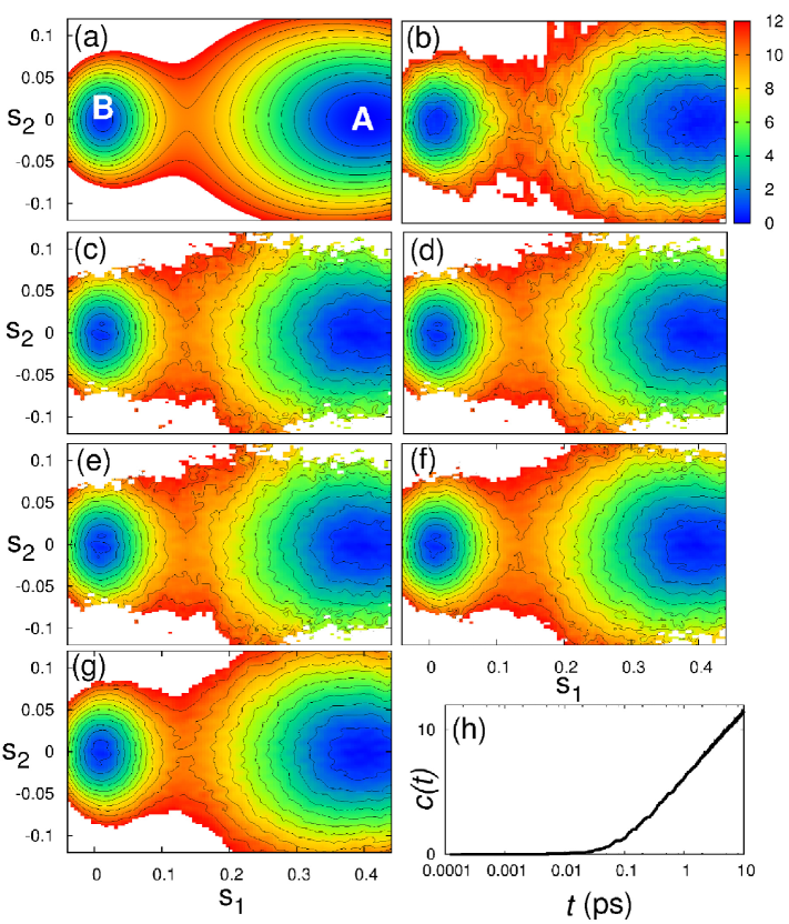
Figure 2: Two–dimensional double well potential: (a) Potential energy surface; (b) free energy surface from two–dimensional WT–MTD; Free energy surfaces from WS–MTD simulations for ($t_{\rm min},t_{\rm max}$) values (in ps): (c) (0.1,1.4), (d) (0.1,2.8), (e) (0.2,1.4), (f) (0.2,2.8), (g) (1.4,11.4); (h) $c(t)$ plot for one of the windows in the WS–MTD simulation where $t$ axis is in log–scale. Free energy values are in kcal mol^-1 relative to the free energy of the broad minimum (A). $c(t)$ is in kcal mol^-1. Contour values are drawn from 1.0 to 12.0 kcal mol^-1 at 1 kcal mol^-1 intervals.

Parameters for the potential are given in Table 1, and the plot of $U(x,y)$ is shown in Figure 2. The two minima are labeled as A (broad minimum) and B (narrow minimum), and the barriers for A$\rightarrow$B and B$\rightarrow$A are 9.8 kcal mol^-1 and 9.3 kcal mol^-1, respectively.

Two different sets of simulations were carried out: (a) WS–MTD simulation with $x$ coordinate chosen as the CV ($s_{1}$) for umbrella sampling and the $y$ coordinate as the CV ($s_{2}$) for one–dimensional WT–MTD sampling; (b) a two–dimensional WT–MTD simulation with CVs $x$, and $y$ coordinates ($s_{1}$, and $s_{2}$, respectively). Umbrella potentials were placed along $s_{1}$ from $-0.05$ to $0.44$ Bohr at intervals of 0.01 Bohr. Restraining potential $\kappa_{h}$ for all the umbrella potentials were 9.9653$\times 10^{3}$ kcal mol^-1 Bohr^-2.

Mass of the particle was taken as 50 a.m.u. and constant temperature simulation was carried out using Anderson thermostat at 300 K. In WS–MTD and two–dimensional WT–MTD simulations, time steps for integrating the equations of motion were chosen as 0.12 and 0.17 fs, respectively. The initial Gaussian height ($w_{0}$) is 0.63 kcal mol^-1 and the hill width parameter $\delta s$ is 0.005 Bohr. $\Delta T$ parameter for the WT–MTD simulations was taken as 1200 K.

Before starting a WS–MTD, we carried out equilibration for a particular umbrella potential (for 2–5 ps), without adding MTD bias. Initial structure for an umbrella (away from the equilibrium) was chosen from the equilibrated structure of the nearest umbrella potential. This strategy has been also used for all the other systems studied here.

2.4.2 1,3–Butadiene to Cyclobutene Reaction

1,3–Butadiene can exist in cis and trans form and by an electrocyclic reaction it forms cyclobutene. Free energy surface has a broad reactant basin and thus is an ideal problem to demonstrate the efficiency of the WS–MTD method using ab initio MD.

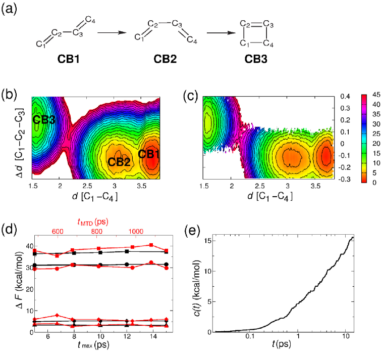
Figure 3: (a) Structure of trans-1,3-butadiene (CB1), cis-1,3-butadiene (CB2), and cyclobutene (CB3). Reconstructed free energy surface for 1,3-butadiene to cyclobutene reaction computed from (b) two–dimensional WT–MTD ($t_{\rm MTD}$=1.2 ns), and (c) WS–MTD ($t_{\rm min}$=0.0, $t_{\rm max}$=15 ps). Free energy values are in kcal mol^-1 relative to the free energy of the minimum (CB1). Contour values are shown from 1.0 to 45.0 kcal mol^-1 for every 2 kcal mol^-1. CVs are in Å. (d) Various free energy barriers (color code: WS–MTD (black), WT–MTD (red)) on the free energy landscape computed for different $t_{\rm max}$ values from WS–MTD simulation (bottom axis) together with the corresponding free energy barriers from two–dimensional WT–MTD with increasing MTD time, $t_{\rm MTD}$ (top axis). Here symbols $\blacksquare$, $\bullet$, $\blacklozenge$, $\blacktriangle$ represent free energy barriers for CB2$\rightarrow$CB3, CB3$\rightarrow$CB2, CB1$\rightarrow$CB2, and CB2$\rightarrow$CB1 respectively. (e) $c(t)-t$ plot for one of the windows in the WS–MTD simulation, where the $t$ axis is in log–scale.

In order to characterize the cis and trans isomers on the free energy landscape and the formation of cyclobutene, we have chosen the following CVs (see also Figure 3a): a) distance C₁–C₄, $d[\mathrm{C}_{1}-\mathrm{C}_{4}]$; b) the difference in the distances C₁–C₂ and C₂–C₃, $\Delta d[\mathrm{C}_{1}-\mathrm{C}_{2}-\mathrm{C}_{3}]$. In WS–MTD simulations, $d$[C₁–C₄] was sampled using US and $\Delta d[\mathrm{C}_{1}-\mathrm{C}_{2}-\mathrm{C}_{3}]$ was sampled using WT–MTD. Two–dimensional WT–MTD simulations were also carried out to sample both CVs simultaneously. WS–MTD and WT–MTD simulations were performed within the framework of ab initio MD using plane–wave Kohn-Sham density functional theory (DFT) employing the CPMD program. [30] PBE exchange correlation functional [31] with ultrasoft pseudopotential [32] was used for these calculations. A cutoff of 30 Ry was used for the plane–wave expansion of wavefunctions. Constant temperature Car–Parrinello [33] MD at 300 K was carried out using Nos$\mathrm{\grave{e}}$–Hoover chain thermostats. [34] A time step of 0.096 fs was used to integrate the equations of motion. A mass of 600 a.u. was assigned to the orbital degrees of freedom. System was taken in a cubic supercell of side length 15 Å. Extended Lagrangian MTD approach was used here with a harmonic coupling constant of 1.0 a.u. to restrain the CVs and collective coordinates, and a mass of 50.0 a.m.u. was assigned to all the CVs. Langevin thermostat with a friction coefficient of 0.001 a.u. was used to maintain the CV temperature to 300 K. In WT–MTD simulations, $w_{0}=0.6$ kcal mol^-1 and $\delta s=$0.05 a.u. were taken. MTD bias was updated every 19 fs. Two independent two–dimensional WT–MTD simulations were performed using $\Delta T=3000$ K and 25000 K. In US, windows were placed from 1.5 Å to 3.9 Å at an interval of 0.05 Å with $\kappa_{\rm h}=1.57\times 10^{3}$ kcal mol^-1 Å^-2. In the case of WS–MTD, $\Delta T=3000$ K was used while all the other MTD parameters were the same as in the case of the normal WT–MTD.

2.4.3 Controlled Sampling of Ligand Exchange in a Pd–Allyl Alcohol Complex in Aqueous Solution

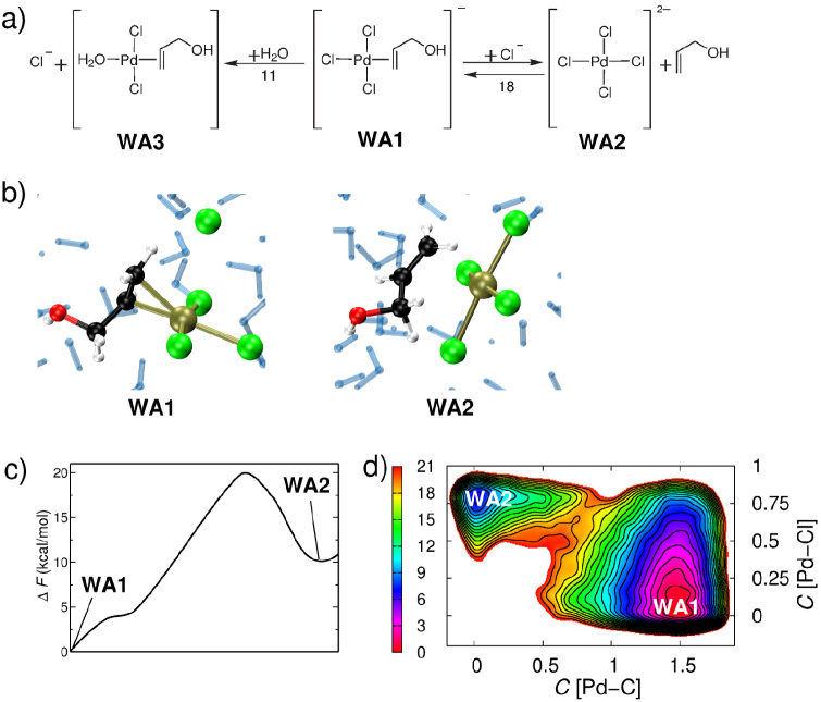
Figure 4: (a) Structure of Pd complex with allyl alcohol (WA1), PdCl${}_{4}^{2-}$ (WA2) and Pd complex with water (WA3). Free energy barriers in kcal mol^-1 are indicated over arrows, as computed from our previous study.[26] (b)Snapshots from the simulation showing the complex of Pd with allyl alcohol (WA1), and PdCl${}_{4}^{2-}$ (WA2); color code: Pd (tan), Cl (green), C (black), O(red), H(white) and solvent water molecules in blue stick representation. (c) Minimum energy pathway traced on the converged five–dimensional free energy landscape. (d) The non reweighted reconstructed free energy surface WA1$\rightarrow$WA2 visualized along the MTD CVs for $C\mathrm{[Pd-Cl_{trans}]}=0.74$ and $C\mathrm{[Pd-O_{w}]}=1.24$. Free Energy values are in kcal mol^-1 relative to the free energy of the minimum (WA1). Contour values are drawn from 1.0 to 20.0 kcal mol^-1 for every 1 kcal mol^-1.

Here we are interested to compute the free energy barrier for the reaction WA1$\rightarrow$WA2 (Figure 4a) in aqueous solution. The purpose of this simulation is to achieve a controlled sampling, in particular, to avoid sampling the rapid ligand exchanges of trans Cl with solvent molecules to form WA3. [26] To simulate this process we have chosen four CVs: a) coordination number Pd to all the oxygen atoms of water molecules, $C\mathrm{[Pd-O_{w}]}$; b) coordination number of Pd to Cl atom that is trans to the coordinated allyl alcohol, $C\mathrm{[Pd-Cl_{trans}]}$; c) coordination number of Pd to the two C atoms of allyl alcohol to which it is coordinated, $C\mathrm{[Pd-C]}$; d) coordination number of Pd to the Cl^- in solution, $C\mathrm{[Pd-Cl]}$. Ab initio MD simulations were performed with the same technical details as mentioned previously. A periodic cubic box having the side length of 12.0 Å containing the WA1 complex, one Cl^-, and 53 water molecules were taken. The equilibrated structure of this system was taken from our previous study in Ref. [26].

We carried out WS–MTD simulations by sampling the CVs $C\mathrm{[Pd-O_{w}]}$ and $C\mathrm{[Pd-Cl_{trans}]}$ by US, and the CVs $C\mathrm{[Pd-C]}$ and $C\mathrm{[Pd-Cl]}$ by WT–MTD. In these simulations, the umbrella windows along the CV $C\mathrm{[Pd-Cl_{{trans}}]}$ were placed at 0.86 and 0.74, with $\kappa_{h}$ 251 kcal mol^-1 and 502 kcal mol^-1, respectively. The position of the umbrella window along the CV $C\mathrm{[Pd-O_{w}]}$ was fixed at 1.24. The $\kappa_{h}$ for the umbrellas along $C\mathrm{[Pd-O_{w}]}$ was 21.3 kcal mol^-1. The position and $\kappa_{h}$ for the umbrella restraints were based on the distribution of these CVs at equilibrium in the WA1 state.

We carried out the extended Lagrangian MTD where a harmonic coupling constant of 2.0 a.u. was used to restrain CVs and collective coordinates, and a CV mass of 50.0 a.m.u was assigned. Temperature of the CV was maintained to 300$\pm$ 200 K by a direct velocity scaling. MTD biasing potential was updated every 29 fs and the MTD parameters $w_{0}=0.62$ kcal mol^-1, and $\delta s=0.05$ were taken. $\Delta T=3000$ K was chosen for these simulations.

As we are only interested in the forward barrier along the MTD CVs, we have used the strategy presented in Section 2.2. Moreover, to trace the minimum energy pathway on the reconstructed five–dimensional free energy surface, we used the string method.[35]

2.4.4 Free Energy for Water Coordination to the Active Site of NDM–1 by QM/MM Simulations

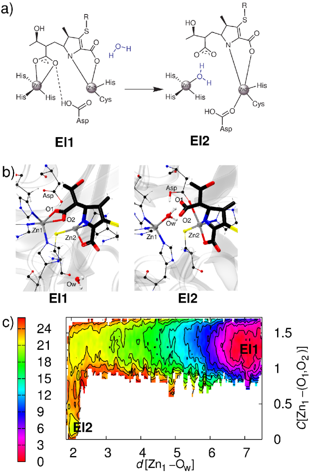
Figure 5: (a) Structures of (EI1) and (EI2) with active site water molecule shown in blue color. (b) Snapshots of EI1, and EI2; color code: Zn (gray), C (black), O (red), N (blue), S (yellow), and H (white). Active site residues and the attacking water molecule are in CPK representation, while the drug molecule is shown in stick representation. (c)Reconstructed free energy computed from WS–MTD. Free energy values are in kcal mol^-1 relative to the free energy of the minimum (EI1). Contour values are drawn from 1 to 26 kcal mol^-1 for every 2 kcal mol^-1. $d$[Zn₁–O_w] is in Å.

To sample the reaction from EI1$\rightarrow$EI2 two CVs were chosen (Figure 5b): a) distance between Zn₁ and to the nearest water molecule (as identified in our earlier work [27]), $d\mathrm{[Zn_{1}-O_{w}]}$; b) coordination number of Zn₁ to the carboxylate oxygen atoms O₁ and O₂, $C\mathrm{[Zn_{1}-(O_{1},O_{2})]}$. The first coordinate was chosen as the US CV as we are expecting a broad and deep free energy basin along this coordinate, while the other coordinate was chosen for the WS–MTD sampling. Umbrella potentials were placed from 7.4 Å to 1.9 Å at an interval of 0.1 Å with $\kappa_{\rm h}=4.5\times 10^{2}$ kcal mol^-1 Å^-2.

Hybrid QM/MM simulations were performed using the CPMD/GROMOS interface [36] as implemented in the CPMD package. The equilibrated structure of EI1 was taken from our previous work [27]; see (Figure 5). Two Zn ions, meropenem drug, side chains of His₁₂₀, His₁₂₂, Asp₁₂₄, His₁₈₉, Cys₂₀₈, and His₂₅₀ and the water molecule near the active site were treated quantum mechanically (QM). Rest of the protein and the solvent molecules were treated by molecular mechanics (MM), and were taken in a periodic box of size 69.0$\times$63.2$\times$66.8 Å³. The whole protein, including the QM part, and the solvent molecules were free to move during the MD simulations. The QM part was treated using the plane–wave DFT with Ultrasoft pseudopotentials and with a plane–wave cutoff of 30 Ry. A QM box size of 27.5$\times$27.8$\times$22.8 Å³ was chosen. Whenever a chemical bond has to be cleaved to define partition between QM and MM parts, boundary atoms are capped using hydrogen atoms. Capping hydrogen atoms were introduced between C_β and C_γ atoms of His₁₂₀, His₁₂₂, His₁₂₉, and His₂₅₀ and C_α and C_β atoms of Asp₁₂₄, and Cys₂₀₈.

Car–Parrinello MD was carried out for the QM part. Time step for the integration of the equations of motion was 0.145 fs. A mass of 700 a.u. was assigned to the orbital degrees of freedom and Nosé–Hoover chain thermostats [34] were used to perform $NVT$ ensemble simulations at 300 K.

Extended Lagrangian variant of MTD was used where harmonic coupling constant was taken as 2.0 a.u. and the CV mass was set to 50.0 a.m.u. CV temperature was maintained to 300 K by coupling to Langevin thermostat with a frictional coefficient of 0.001 a.u. Gaussian potentials were updated every 29 fs and the MTD parameters $w_{0}=0.62$ kcal mol^-1, $\delta s=0.05$ and $\Delta T=7500$ K were taken. We followed the strategy described in Section 2.2 for reweighting the CV space near the transition state along the MTD CV.

3 Results and Discussion

First we benchmark the accuracy of WS–MTD method by sampling a two–dimensional model system where the free energy barriers are exactly known (Section 3.1). To demonstrate the efficiency of WS–MTD simulation over the WT–MTD simulation in sampling broad and deep free energy wells, we model the cyclization reaction of 1,3–butadiene using ab initio MD (Section 3.2). In Section 3.3, we demonstrate a controlled sampling of a high–dimensional surface using WS–MTD, which is otherwise difficult using normal MTD. Subsequently, we present an example where WS–MTD is used together with QM/MM methods to sample the broad free energy surface of an enzymatic reaction, for which normal MTD simulations have failed.

3.1 Two Dimensional Model System

We carried out a two–dimensional WT–MTD simulation starting from the minimum A using the CVs $s_{1}(\equiv x)$ and $s_{2}(\equiv y)$. Several re-crossings were observed in the WT–MTD simulation, while a proper convergence in the barriers was observed by the third recrossing at 86.7 ps. The converged free energy barriers for A$\rightarrow$B and B$\rightarrow$A are 9.8 and 9.3 kcal mol^-1, respectively, and are identical to the exact barriers from the potential energy surface (Figure 2a). Free energy surface from this simulation is shown in Figure 2b. We then carried out WS–MTD simulations, by sampling $s_{1}$ and $s_{2}$ using US and one–dimensional WT–MTD simulation, respectively. During these simulations, $c(t)$ values for all the 50 umbrella windows were computed according to Equation (11). For all the umbrellas, $c(t)$–$t$ plots were nearly identical, and one of the plots is shown in Figure 2h. $c(t)\propto\ln(t)$ behavior was observed for $t>0.1$ ps for all the umbrella windows. Thus, for reweighting the MTD simulations using Equation (13), we tested various values of $t_{\rm min}$ and $t_{\rm max}$ greater than 0.1 ps, and the resulting free energy surfaces were analyzed for convergence in free energy barriers. For $t_{\rm min}=0.1$ ps and $t_{\rm max}=0.6$ ps, the reconstructed free energy surface was quite noisy, and the free energy barriers are having an error upto 0.4 kcal mol^-1 (Table 2). On the other hand, for $t_{\rm max}=1.4$ ps, free energy barriers for A$\rightarrow$B and B$\rightarrow$A were 9.8 and 9.2 kcal mol^-1, respectively, which is in good agreement with the reference free energy barriers; see also Figure 2c. The topology of the relevant parts of the free energy surface is also well reproduced. For higher $t_{\rm max}$ values, the free energy barriers converge to the exact values (Table 2). The same convergence behavior was also observed for $t_{\rm min}>0.1$ ps. It is also interesting to note that $t_{\rm min}=0.0$ and $t_{\rm max}=1.4$ also gave reasonably accurate free energy barriers; see also the figure in the supporting information where error in the free energy barriers as a function of cumulative simulation time is shown for both WS–MTD and WT–MTD. Thus, performances of WS–MTD and WT–MTD are nearly the same, but the advantage of WS–MTD will become more obvious in the realistic examples discussed later. In cases with large $t_{\rm max}$, parts of the surfaces with higher free energy are better explored; see Figure 2d,f,g. However, higher free energy regions are not often interesting and $t_{\rm max}$ could be chosen based on convergence in the computed free energy barriers in more complex realistic systems.

3.2 1,3–Butadiene to Cyclobutene Reaction

Here we carried out a WS–MTD simulation starting with a 1,3–butadiene structure (Figure 3a). The converged reconstructed free energy surface from this simulation is shown in (Figure 3c), where three minima CB1, CB2, CB3 could be observed corresponding to trans-buta-1,3-diene, cis-buta-1,3-diene and cyclobutene, respectively. In WS–MTD, the converged barriers for going from CB1$\rightarrow$CB2 and CB2$\rightarrow$CB1 are 5.3 and 3.3 kcal mol^-1, respectively. The free energy barriers for CB2$\rightarrow$CB3 and CB3$\rightarrow$CB2 are 37.4 and 31.4 kcal mol^-1, respectively (Figure 3c,d). Convergence in all the free energy barriers is achieved with $t_{\rm min}=0.0$ ps and $t_{\rm max}=5.0$ ps (for all the umbrella potentials); see Supporting Information for a more detailed analysis.

To compare the performance of a two–dimensional WT–MTD sampling of both CVs, we carried out two independent WT–MTD simulations with two different $\Delta T$ parameters. In the first simulation, $\Delta T$ was taken as 3000 K, which is the same as that was used for WS–MTD. In this case, even after 1.2 ns of the simulation, no crossing for CB2$\rightarrow$CB3 was seen (see Supporting Information). The failure of WT–MTD is due to the presence of broad and deep reactant well and small $\Delta T$ parameter. Thus a second WT–MTD simulation was then carried out with $\Delta T=25000$ K, where we were successful in seeing several re-crossings from CB2$\rightarrow$CB3 within 1.2 ns. Although free energy barriers for CB1$\rightarrow$CB2 and CB2$\rightarrow$CB1 have converged systematically (due to the small barriers separating them), the free energy barriers for CB2$\rightarrow$CB3 and CB3$\rightarrow$CB2 are not converged to the extent in WS–MTD simulations even after 1.2 ns (Figure 3d). Free energy barriers computed from WS–MTD are well converged within 5.0 ps simulation, but not for WT–MTD even after 1.2 ns. Since we used 49 windows and $t_{\rm max}=5$ ps per umbrella, the total computational time invested for a well converged result in WT–MTD is 245 ps. Also, note that all the 49 windows were running in parallel in our computations and the clock time to complete a converged WS–MTD was equivalent to the clock time required required for simulating 5.0 ps trajectory of a two–dimensional WT–MTD on same number of processors allocated per umbrella.

We thus clearly show for a realistic system, that WS–MTD has better performance over the normal WT–MTD in sampling free energy surfaces with broad and deep basins.

3.3 Controlled Sampling of Ligand Exchange in a Pd–Allyl Alcohol Complex in Aqueous Solution

In our earlier work on the investigation of the Wacker oxidation of allyl alcohol [26] in aqueous solution we were interested in modeling WA1$\rightarrow$WA2. However, we were unable to simulate this step using normal MTD due to rapid ligand exchange reaction of the trans–Cl (Cl_trans) with water molecules from solution, as a result of the strong trans–directing nature of the olefinic group (Figure 4a). Different wall potentials at different values of Pd–Cl_trans coordination number were resulting in different free energy barriers and thus a reliable estimation could not be made. Thus, our earlier work[26] has used the equilibrium constant for WA2$\leftrightharpoons$WA1 from experiment and the barrier for WA2$\rightarrow$WA1 computed from MTD to estimate the WA1$\rightarrow$WA2 barrier as $\approx$19 kcal mol^-1.

In order to compute the free energy barrier for WA1$\rightarrow$WA2, we have sampled the $C\mathrm{[Pd-C]}$, $C\mathrm{[Pd-Cl]}$, $C\mathrm{[Pd-Cl_{trans}]}$ and $C\mathrm{[Pd-O_{w}]}$. The controlled sampling of the $C\mathrm{[Pd-Cl_{trans}]}$ and $C\mathrm{[Pd-O_{w}]}$ CVs was achieved by using US while the other CVs were sampled by a two–dimensional WT–MTD. The restraining values of US coordinates were determined form equilibrium simulation, and the restraining potential was computed from the standard deviation of the probability distribution of these CVs without any MTD bias. Along the $C\mathrm{[Pd-O_{w}]}$ coordinate, we do not want to sample other umbrella windows in order to prevent water coordination and thus the reaction to WA3. Based on our chemical intuition and from our previous experience,[26] we interpret that $C\mathrm{[Pd-Cl_{trans}]}$ could vary from the equilibrium value along the reaction, because when external Cl^- approaches axially and coordinate to Pd, an increase in the Pd–Cl_trans distance is expected. Thus we sampled another overlapping window for the $C\mathrm{[Pd-Cl_{trans}]}$ CV at a lower value (Section 2.4.3). In this way, we carried out WS–MTD simulation to sample only the crucial part of the five–dimensional free energy landscape. Minimum energy pathway on this high–dimensional landscape was then obtained by the string method (Figure 4c). [35]

Since reactant and product basins are present in the MTD CV space (see also Figure 4d) and that we are only interested in obtaining the forward barrier i.e. for the reaction WA1$\rightarrow$WA2, we used the iterative approach for reweighting as discussed in Section 2.2. The convergence in free energy barriers with number of iterations is given in Table 3. A reasonable convergence was obtained for the third iteration, and free energy barrier for WA1$\rightarrow$WA2 is computed as 20 kcal mol^-1 (Figure 4c). This is in excellent agreement with the estimated barrier of 19 kcal mol^-1 in our earlier work. [26]

By presenting this non–trivial example, we demonstrate that WS–MTD can be applied for a controlled sampling of a high–dimensional free energy landscape of a complex reaction. Moreover, the iterative scheme for reweighting the near transition state regions is demonstrated for a realistic system.

3.4 Free Energy for Water Coordination to the Active Site of NDM–1 by QM/MM Simulations

In this section, we study a problem which is part of our ongoing research in elucidating the mechanistic details of antibiotic resistance in NDM–1. [27] In the intermediate stage of one of the proposed mechanisms for the hydrolysis of the acyl–enzyme complex within the active site requires a water molecule to enter the active site and coordinate to the Zn₁ site, further leading to the dissociation of drug–carboxylate group coordination to Zn₁ and subsequent protonation of $\beta$–lactam N (see Figure 5a). [27] We attempted nearly 10 different MTD simulations with various collective variables to model the entry of a QM water to the active site and its coordination to Zn₁, however, they all failed to simulate the reaction, and hinted a broad reactant basin.

Thus, we addressed this problem using WS–MTD by US along $d\mathrm{[Zn_{1}-O_{w}]}$ and WT–MTD sampling along $C\mathrm{[Zn_{1}-(O_{1},O_{2})]}$. The US windows at $d\mathrm{[Zn_{1}-O_{w}]}>2.5$ Å was only simulated till the $\dot{V}^{\rm b}(s,t)\approx 0$ limit is achieved in the relevant values of the $C\mathrm{[Zn_{1}-(O_{1},O_{2})]}$ coordinate. MTD biases are added for the windows with $d\mathrm{[Zn_{1}-O_{w}]}<2.5$ Å till a transition is observed along $C\mathrm{[Zn_{1}-(O_{1},O_{2})]}$ or till the total bias is equal to 25 kcal mol^-1 along the $C\mathrm{[Zn_{1}-(O_{1},O_{2})]}$ coordinate. If a transition is observed along the $C\mathrm{[Zn_{1}-(O_{1},O_{2})]}$ coordinate, we carried out the iterative approach for reweighting the transition state regions of the CV space as mentioned in Section 2.2.

The reconstructed free energy surface thus obtained is given in Figure 5c. The converged free energy barrier for this reaction is 23.6 kcal mol^-1. From the topology of the surface, it is now clear why the normal MTD simulations failed: the free energy basin is deep and flat along the $d\mathrm{[Zn_{1}-O_{w}]}$ coordinate, and the minimum of the reactant basin is at $d\mathrm{[Zn_{1}-O_{w}]}\approx 7$ Å. Free energy surface also indicates that water coordination to Zn₁ and dissociation of Zn₁–carboxylate bond occur in tandem.

4 Conclusions

Based on a combination of Tiwary–Parrinello and US reweighting techniques within WHAM, we propose the WS–MTD strategy for reconstructing complex free energy landscapes by sampling them by slices. Having the advantage of controlling the sampling along a few selected coordinates, WS–MTD aids in efficient sampling of flat, broad and unbound free energy wells with hidden orthogonal barriers. We also propose a simple strategy to reweight MTD trajectories for the regions near the transition state along the MTD CVs in order to obtain converged forward barriers without the need of sampling recrossing trajectories. The WS–MTD also has the advantage of parallelization over umbrellas. This feature enables sampling of high–dimensional landscapes in affordable clock time employing more computational resources in parallel. WS–MTD does not require any special implementation in MD codes that can simultaneously perform restrained dynamics and WT–MTD.

We carried out careful study on the accuracy of the method by sampling a two dimensional model potential where the free energy barriers are exactly known. Free energy barriers were found to converge systematically to the exact values with increasing $t_{\rm max}$. Several applications using the WS–MTD method were then presented. Efficiency of WS–MTD in sampling broad and flat free energy surface is demonstrated by studying the cyclization of 1,3–butadiene using ab initio MD. WS–MTD yields converged free energy barriers with a much less computational cost (by a factor of 5 at least for this problem) than a normal MTD. By sampling the five–dimensional free energy surface for a ligand exchange reaction in a Pd–allyl alcohol complex solvated in water, we demonstrate the application of WS–MTD in controlled sampling of a high dimensional surface. The modeled ligand exchange reaction was earlier reported to fail using normal MTD. Also we showed the application of an iterative approach to reweight the MTD trajectories near the transition state regions on the CV space without the need of simulating multiple recrossing trajectories. Finally, we apply WS–MTD to sample an enzymatic reaction using QM/MM technique, where the coordination of a catalytic water to the active site of NDM–1 enzyme is simulated. For this problem, WS–MTD could efficiently sample broad and deep free energy basins, which was otherwise unable to achieve in a normal MTD after several attempts.

Since the method is practically applicable in ab initio MD and QM/MM MD simulations, we believe that this would be useful for sampling high-dimensional free energy landscape of complex chemical reactions. The technique would be beneficial for various problems in chemistry and biology such as A+B type reactions in weakly bound molecular complexes, reactions in Michaelis complexes, and substrate binding in enzymes to name a few, where one encounters broad and deep free energy basins.

Supporting Information

Supporting information has the following data: a) table analyzing the free energy convergence in WS–MTD and WT–MTD simulations of 1,3–butadiene to cyclobutene reaction; b) a plot showing the convergence of error as a function of cumulative time for WS–MTD and WT–MTD for the two–dimensional model potential; c) details on the computation of correlation time for the two umbrella windows used for the problem in Section 3.3.

Table 1: Parameters for the two–dimensional model potential

$i$	$U_{i}^{o}$ (kcal mol-1)	$a_{i}$ (Bohr-2)	$x_{i}^{o}$ (Bohr)	$y_{i}^{o}$ (Bohr)
1	-17.885	139.2985	0.0000	0.00000
2	-11.625	41.7895	0.3642	0.00000
3	-11.625	41.7895	0.4916	0.00000
4	-11.625	41.7895	0.6189	0.00000
5	-17.885	13.9298	0.1821	0.00000

Table 2: Free energy convergence in WS–MTD simulations for the double–well potential. The converged free energy barriers from 86.7 ps of two–dimensional WT–MTD and the exact free energy values from the potential are also provided for comparison.

Method	$t_{\rm min}$ (ps)	$t_{\rm max}$ (ps)	$\Delta F^{\ddagger}$ (kcal mol-1)
			A$\rightarrow$ B	B$\rightarrow$ A
WS–MTD	0.0	0.6	10.5	9.5
		1.4	10.0	9.2
		2.8	9.9	9.3
	0.1	0.6	10.1	8.8
		1.4	9.8	9.2
		2.8	9.8	9.3
	0.2	1.4	9.7	9.1
		2.8	9.8	9.3
	1.5	10.0	9.8	9.3
WT–MTD	-	-	9.8	9.3
Exact	-	-	9.8	9.3

Table 3: Convergence in the computed forward free energy barriers for WA1$\rightarrow$WA2 with number of iterations.

Iteration	$\Delta F^{\ddagger}$ (kcal mol-1)
1	19.4
2	19.9
3	20.1

Table of Content Figure:

Abstract for the Table of Content Figure:

Here we present a technique to sample a high–dimensional free energy landscape as slices by combining umbrella sampling and metadynamics simulation sampling orthogonal coordinates simultaneously. The full free energy surface is then reconstructed by combining these slices using the Weighted Histogram Analysis Method.

References

- [1] A. Laio, M. Parrinello, Proc. Natl. Acad. Sci. 2002, 99, 12562–12566.
- [2] M. Iannuzzi, A. Laio, M. Parrinello, Phys. Rev. Lett. 2003, 90, 238302.
- [3] A. Barducci, M. Bonomi, M. Parrinello, WIREs Comput. Mol. Sci. 2011, 1, 826–843.
- [4] L. Sutto, S. Marsili, F. L. Gervasio, WIREs: Comput. Mol. Sci. 2012, 2, 771–779.
- [5] A. Laio, F. L. Gervasio, Rep. Prog. Phys. 2008, 71, 126601.
- [6] A. Barducci, G. Bussi, M. Parrinello, Phys. Rev. Lett. 2008, 100, 020603.
- [7] J. F. Dama, M. Parrinello, G. A. Voth, Phys. Rev. Lett. 2014, 112, 240602.
- [8] G. Bussi, F. L. Gervasio, A. Laio, M. Parrinello, J. Am. Chem. Soc. 2006, 128, 13435–13441.
- [9] S. Piana, A. Laio, J. Phys. Chem. B 2007, 111, 4553–4559.
- [10] F. Marinelli, F. Pietrucci, A. Laio, S. Piana, PLOS Comput. Biol. 2009, 5, e1000452.
- [11] G. M. Torrie, J. P. Valleau, Chem. Phys. Lett. 1974, 28, 578–581.
- [12] A. M. Ferrenberg, R. H. Swendsen, Phys. Rev. Lett. 1989, 63, 1195–1198.
- [13] S. Kumar, D. Bouzida, R. H. Swendsen, P. A. Kollman, J. M. Rosenberg, J. Comput. Chem. 1992, 13, 1011–1021.
- [14] M. McGovern, J. de Pablo, J. Chem. Phys. 2013, 139, 084102.
- [15] F. P. Y. Crespo, F. Marinelli, A. Laio, Phys. Rev. B 2010, 81, 055701.
- [16] G. Tiana, Eur. Phys. J. B 2008, 63, 235–238.
- [17] M. Bonomi, A. Barducci, M. Parrinello, J. Comput. Chem. 2009, 30, 1615–1621.
- [18] P. Tiwary, M. Parrinello, J. Phys. Chem. B 2014, 119, 736–742.
- [19] J. M. Johnston, H. Wang, D. Provasi, M. Filizola, PLoS Comp. Biol. 2012, 8, e1002649.
- [20] J. Kästner, WIREs Comput. Mol. Sci. 2011, 1, 932–942.
- [21] M. Yang, L. Yang, Y. Gao, H. Hu, J. Chem. Phys. 2014, 141, 044108.
- [22] B. Ensing, A. Laio, M. Parrinello, M. L. Klein, J. Phys. Chem. B 2005, 109, 6676–6687.
- [23] V. Babin, C. Roland, T. A. Darden, C. Sagui, J. Chem. Phys. 2006, 125, 204909.
- [24] E. Autieri, M. Sega, F. Pederiva, G. Guella, J. Chem. Phys. 2010, 133, 095104.
- [25] Y. Zhang, G. A. Voth, J. Chem. Theory Comput. 2011, 12, 2277–2283.
- [26] V. Imandi, N. N. Nair, J. Phys. Chem. B 2015, 119, 11176–11183.
- [27] R. Tripathi, N. N. Nair, ACS Catal. 2015, 5, 2577–2586.
- [28] D. Branduardi, G. Bussi, M. Parrinello, J. Chem. Theory Comput. 2012, 8, 2247–2254.
- [29] J. S. Hub, B. L. de Groot, D. van der Spoel, J. Chem. Theory Comput. 2010, 6, 3713–3720.
-
[30]
Version 13.2, CPMD Program Package, IBM Corp 1990-2011, MPI
für Festkörperforschung Stuttgart 1997-2001,
see also http://www.cpmd.org. - [31] J. P. Perdew, J. A. Chevary, S. H. Vosko, K. A. Jackson, M. R. Pederson, D. J. Singh, C. Fiolhais, Phys. Rev. B 1992, 46, 6671–6687.
- [32] D. Vanderbilt, Phys. Rev. B 1990, 41, 7892–7895.
- [33] R. Car, M. Parrinello, Phys. Rev. Lett. 1985, 55, 2471–2474.
- [34] G. J. Martyna, M. L. Klein, M. Tuckermann, J. Chem. Phys. 1992, 97, 2635.
- [35] W. E, W. Ren, E. Vanden-Eijnden, Phys. Rev. B 2002, 66, 052301.
- [36] A. Laio, J. VandeVondele, U. Rothlisberger, J. Chem. Phys. 2002, 116, 6941–6947.