Quantum integrable combinatorics of Schur polynomials

Abstract

We examine and present new combinatorics for the Schur polynomials from the viewpoint of quantum integrability. We introduce and analyze an integrable six-vertex model which can be viewed as a certain degeneration model from a $t$-deformed boson model. By a detailed analysis of the wavefunction from the quantum inverse scattering method, we present a novel combinatorial formula which expresses the Schur polynomials by using an additional parameter, which is in the same sense but different from the Tokuyama formula. We also give an algebraic analytic proof for the Cauchy identity and make applications of the domain wall boundary partition functions to the enumeration of alternating sign matrices.

1 Introduction

Schur polynomials is an ubiquitous object in mathematics and mathematical physics, ranging from representation theory, combinatorics, enumerative geometry to knot theory. Being one of the most fundamental symmetric polynomials, extensive studies and numerous combinatorial identities have been found for the Schur polynomials. Many mathematical objects are introduced for which the Schur polynomials serves as a building block since one can use various properties found for the Schur polynomials. One typical example is a stochastic process called the Schur process [1] whose probability measure is given by the Schur polynomials, from its property many useful combinatorial formulae can be employed to study the dynamics of the process.

The Schur polynomials itself has many expressions. One of the most famous ones is the Jacobi-Trudi identity which expresses Schur polynomials in terms of elementary symmetric polynomials. Besides these traditional identities, a very interesting formula called the Tokuyama formula [2, 3, 4] was found which expresses Schur polynomials in a combinatorial form. The distinctive feature of the formula is that the expression is given in terms not only of the symmetric variables but also with an additional parameter which does not appear in the original definition of the Schur polynomials. Specializing the additional parameter, the Tokuyama formula reduces to the determinant formula, Weyl character formula and so on. In this sense, the Tokuyama formula can be viewed as a deformation of Weyl character.

Recently, the Tokuyama formula has found its interpretation in terms of integrable vertex models [5]. The idea to understand this Tokuyama formula from the point of view of quantum integrability is to extend the $L$-operator for the free-fermion model (the corresponding $R$-matrix is the trigonometric Felderhof model) to an $L$-operator including an additional parameter besides the spectral parameter. The newly-introduced parameter plays the role of refining the combinatorial expression for the Schur polynomials. This idea of relating Tokuyama formula which is a deformation of Weyl character formula to integrable vertex models have been recently generalized to the factorial Schur polynomials [6] and other types of symmetric polynomials [7, 8, 9, 10] by introducing inhomogeneous parameters or changing boundary conditions.

In this paper, we present another type of combinatorial formula for the Schur polynomials with an additional parameter by investigating a partition function of an integrable six-vertex model. We find the following combinatorial formula for the Schur polynomials

$$s_{\lambda}(\boldsymbol{z})= \frac{1}{\prod_{1\leq j<k\leq N}(z_{j}+z_{k}+2\beta z_{j}z_{k})}\sum_{x^{(N)}\succ x^{(N-1)}\succ\dots\succ x^{(0)}=\phi}\prod_{k=1}^{N}\Bigg{\{}z_{k}^{\sum_{j=1}^{k}x_{j}^{(k)}-\sum_{j=1}^{k-1}x_{j}^{(k-1)}-1}$$

$$\times \Bigg{(}\frac{2(1+\beta z_{k})}{1+2\beta z_{k}}\Bigg{)}^{\#(x^{(k)}|x^{(k-1)})-1}\prod_{j=1}^{k-1}\Bigg{(}1+2\beta z_{k}(1-\delta_{x_{j}^{(k-1)}x_{j+1}^{(k)}})\Bigg{)}\Bigg{\}},$$ (1.1)

where $\beta$ is an arbitrary parameter. $x^{(k)}=(x_{1}^{(k)},\dots,x_{k}^{(k)})$, $k=1,\dots,N$ are strict partitions satisfying the interlacing relations $x^{(N)}\succ x^{(N-1)}\succ\dots\succ x^{(0)}=\phi$, $x^{(N)}$ is fixed by the Young diagram $\lambda=(\lambda_{1},\dots,\lambda_{N})$ as $\lambda_{j}=x_{j}^{(N)}-N+j-1$, and $\#(y|x)$ denotes the number of parts in $y$ which are not in $x$.

We obtain this combinatorial formula from an integrable six-vertex model. The six-vertex model we consider can be regarded as a certain degeneration of a $t$-deformed non-Hermitian boson model introduced in [11]. The corresponding wavefunction seems to be analyzed by the coordinate Bethe ansatz [12] which at the degeneration point is given by the Schur polynomials times a factor including an additional parameter. To obtain the combinatorial formula (1.1), we investigate the corresponding model from the point of view of the quantum inverse scattering method, i.e., starting from the $L$-operator which is the most fundamental object in quantum integrable models. We view the wavefunction as a partition function of a six-vertex model and evaluate it in two ways. First, we evaluate the partition function directly to show that it is given by a Schur polynomials times an additional factor. Another way of evaluation is to take the viewpoint that the partition function consists of a layer of $B$-operators, and calculate the matrix elements of a single $B$-operator to show a summation formula for the partition function. Combining the two expressions give the combinatorial formula (1.1).

Besides the combinatorial formula, we examine the scalar products and present an algebraic analytic proof for its determinant form, which combined with the wavefunction gives us the celebrated Cauchy formula for the Schur polynomials. We also make an application of the domain wall boundary partition function to show a simple formula for a particular generating function of alternating sign matrices.

This paper is organized as follows. We introduce the integrable six-vertex model as a particular degeneration of a non-Hermitian $t$-deformed boson model in the next section. We give an algebraic analytic proof for the scalar product in section 3. In sections 4 and 5, we evaluate the matrix elements and the wavefunction of the six-vertex model. We combine the results of sections 3, 4 and 5 to present the combinatorial formulae for the Schur polynomials in section 6. In section 7, we give an application of the domain wall boundary partition function to a generating function of the alternating sign matrices.

2 Non-Hermitian $t$-deformed boson model and reduction to the six-vertex model

We introduce the $t$-deformed non-Hermitian boson model [11, 12] and its equivalent six-vertex model at the point $t=-1$. The model is characterized by $t$-deformed boson algebra with generators $N,B,B^{\dagger}$ satisfying the following relations

$$[B,B^{\dagger}]=t^{N}(1-t),\quad[N,B]=-B,\quad[N,B^{\dagger}]=B^{\dagger}.$$ (2.1)

These generators act on a Fock space $\mathcal{F}$ spanned by the orthonormal basis $|n\rangle\ (n\geq 0)$ as

$$B|n\rangle=|n-1\rangle,\ B^{\dagger}|n\rangle=(1-t^{n+1})|n+1\rangle,\ N|n\rangle=n|n\rangle.$$ (2.2)

The operators the dual orthonormal basis $\langle n|$ ($n\geq 0$) satisfying $\langle n|m\rangle=\delta_{nm}$ as

$$\langle n|B^{\dagger}=(1-t^{n})\langle n-1|,\ \langle n|B=\langle n+1|,\ \langle n|N=n\langle n|.$$ (2.3)

We consider the following $L$-operator which is a slightly deformation of the one in [11]

$$\mathcal{L}_{aj}(v)=\begin{pmatrix}1-\beta vt^{N_{j}}&vB_{j}^{\dagger}\\ B_{j}&v\end{pmatrix}_{a},$$ (2.4)

acting on the tensor product $W_{a}\otimes\mathcal{F}_{j}$ of the complex two-dimensional space $W_{a}$ and the Fock space at the $j$th site $\mathcal{F}_{j}$. Let us denote the orthonormal basis of $W_{a}$ and its dual as $\{|0\rangle_{a},|1\rangle_{a}\}$ and $\{{}_{a}\langle 0|,{}_{a}\langle 1|\}$. The explicit forms of the matrix elements of (2.4) in the orthonormal basis are

$${}_{a}\langle 0|{}_{j}\langle m_{j}|\mathcal{L}_{aj}(v)|0\rangle_{a}|n_{j}\rangle_{j} =(1-\beta vt^{n_{j}})\delta_{m_{j},n_{j}},$$ (2.5)

$${}_{a}\langle 1|{}_{j}\langle m_{j}|\mathcal{L}_{aj}(v)|0\rangle_{a}|n_{j}\rangle_{j} =\delta_{m_{j},n_{j}-1},$$ (2.6)

$${}_{a}\langle 0|{}_{j}\langle m_{j}|\mathcal{L}_{aj}(v)|1\rangle_{a}|n_{j}\rangle_{j} =v(1-t^{n_{j}+1})\delta_{m_{j},n_{j}+1},$$ (2.7)

$${}_{a}\langle 1|{}_{j}\langle m_{j}|\mathcal{L}_{aj}(v)|1\rangle_{a}|n_{j}\rangle_{j} =v\delta_{m_{j},n_{j}}.$$ (2.8)

In figure 1, we depict the non-zero elements of the $L$-operator.

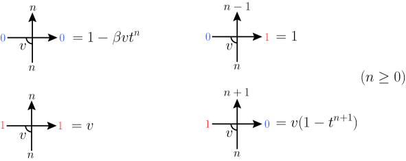
Figure 1: The non-zero elements of the $L$-operator.

The $L$-operator satisfies the intertwining relation ($RLL$-relation)

$$R_{ab}(u,v)\mathcal{L}_{aj}(u)\mathcal{L}_{bj}(v)=\mathcal{L}_{bj}(v)\mathcal{L}_{aj}(u)R_{ab}(u,v),$$ (2.9)

which acts on $W_{a}\otimes W_{b}\otimes\mathcal{F}_{j}$. The $R$-matrix

$$R(u,v)=\begin{pmatrix}u-tv&0&0&0\\ 0&t(u-v)&(1-t)u&0\\ 0&(1-t)v&u-v&0\\ 0&0&0&u-tv\end{pmatrix},$$ (2.10)

is a solution to the Yang-Baxter equation:

$$R_{ab}(u,v)R_{ac}(u,w)R_{bc}(v,w)=R_{bc}(v,w)R_{ac}(u,w)R_{ab}(u,v).$$ (2.11)

From the $L$-operator, we construct the monodromy matrix

$$\mathcal{T}_{a}(v)=\prod_{j=1}^{M}\mathcal{L}_{aj}(v),$$ (2.12)

which acts on $W_{a}\otimes(\mathcal{F}_{1}\otimes\dots\otimes\mathcal{F}_{M})$. Tracing out the auxiliary space, one defines the transfer matrix $\tau(v)\in\mathrm{End}(\mathcal{F}^{\otimes M})$:

$$\tau(v)=\operatorname{Tr}_{W_{a}}\mathcal{T}_{a}(v).$$ (2.13)

Simplifications happen for the $t$-deformed boson model at $t=-1$. Due to the matrix element (2.7), when we construct $N$-particle states from the vacuum, each site can only be occupied by at most one boson. This is equivalent to the reduction of the $t$-deformed boson model to the six-vertex model whose $L$-operator is given by

$$\mathcal{L}_{aj}(v)=\begin{pmatrix}1-\beta v&0&0&0\\ 0&1+\beta v&2v&0\\ 0&1&v&0\\ 0&0&0&v\end{pmatrix}_{aj}.$$ (2.14)

One can check that (2.14) indeed satisfies the intertwining relation (2.9). We analyze the structure of this six-vertex model in this paper. We remark that at the other degenerated point $t=0$ of the $t$-deformed boson model, the model is called the non-Hermitian phase model [13], whose wavefunction [14] constructed from the $L$-operator is given by the Grothendieck polynomials [15, 16, 17, 18, 19], which furthermore reduces to the Schur polynomials by taking $\beta=0$ where the corresponding model is the Hermitian phase model [20, 21, 22, 23]. On the other hand, the wavefunction at $\beta=0$ for generic $t$ is given by the Hall-Littlewood polynomials [24, 25].

3 Scalar Products of state vectors of the six-vertex model

In this section, we first construct a state vector of the integrable $t$-deformed boson model following the standard procedure of the quantum inverse scattering method (i.e. the algebraic Bethe ansatz) which is based on the Yang-Baxter algebra. The $N$-particle state $|\Psi(\{v\}_{N})\rangle$ is characterized by $N$ unknown numbers $v_{j}\in\mathbb{C}$ ($1\leq j\leq N$), and is not an eigenvector of the transfer matrix in general. However, if the parameters $v_{j}$ satisfy a set of constraints called the Bethe ansatz equation, the $N$-particle state becomes an eigenstate. We call the state $|\Psi(\{v\}_{N})\rangle$ on-shell state if $\{v\}$ satisfies the Bethe ansatz equation, and off-shell state if no constraints are imposed on $\{v\}$. We then restrict the analysis to $t=-1$, which is equivalent to considering the six-vertex model (2.14), and prove the determinant form for the scalar products $\langle\Psi(\{u\}_{N})|\Psi(\{v\}_{N})\rangle$ which is the inner product between the off-shell state $|\Psi(\{v\}_{N})\rangle$ and the dual off-shell state $\langle\Psi(\{u\}_{N})|$.

From the $L$-operator, we construct the monodromy matrix

$$\mathcal{T}_{a}(v,\{w\})=\prod_{j=1}^{M}\mathcal{L}_{aj}(v/w_{M+1-j})=\begin{pmatrix}\mathcal{A}(v,\{w\})&\mathcal{B}(v,\{w\})\\ \mathcal{C}(v,\{w\})&\mathcal{D}(v,\{w\})\end{pmatrix}_{a},$$ (3.1)

which acts on $W_{a}\otimes(\mathcal{F}_{1}\otimes\dots\otimes\mathcal{F}_{M})$. Here we introduced the inhomogeneous parameters $w_{1},\dots,w_{M}\in\mathbb{C}$. See figure 2 for the graphical description of the elements of the monodromy matrix.

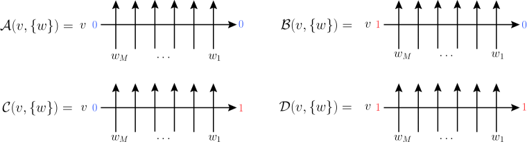
Figure 2: The diagrammatic representation of the elements of the monodromy matrix (3.1) with inhomogeneous parameters $w_{M+1-j}$ associated with site $j$.

Taking the homogeneous limit $w_{j}\to 1$ ($1\leq j\leq M$), (2.12) is recovered:

$$\mathcal{T}_{a}(v,\{w\})|_{w_{1}=1,\dots,w_{M}=1}=\mathcal{T}_{a}(v).$$ (3.2)

As in the above equation, hereafter we will omit $\{w\}$ for the quantities in the homogeneous limit (e.g. $\mathcal{A}(v):=\mathcal{A}(v,\{w\})|_{w_{1}=1,\dots,w_{M}=1}$). Tracing out the auxiliary space, one defines the transfer matrix $\tau(v,\{w\})\in\mathrm{End}(\mathcal{F}^{\otimes M})$:

$$\tau(v,\{w\})=\operatorname{Tr}_{W_{a}}\mathcal{T}_{a}(v,\{w\}).$$ (3.3)

The repeated applications of the $RLL$-relation leads to the intertwining relation

$$R_{ab}(u,v)\mathcal{T}_{a}(u,\{w\})\mathcal{T}_{b}(v,\{w\})=\mathcal{T}_{b}(v,\{w\})\mathcal{T}_{a}(u,\{w\})R_{ab}(u,v).$$ (3.4)

Some of the elements of the intertwining relation are

$$\mathcal{C}(u,\{w\})\mathcal{B}(v,\{w\})-t\mathcal{B}(v,\{w\})\mathcal{C}(u,\{w\})$$

$$=g(u,v)(\mathcal{A}(v,\{w\})\mathcal{D}(u,\{w\})-\mathcal{A}(u,\{w\})\mathcal{D}(v,\{w\})),$$ (3.5)

$$\mathcal{A}(u,\{w\})\mathcal{B}(v,\{w\})=f(u,v)\mathcal{B}(v,\{w\})\mathcal{A}(u,\{w\})+g(u,v)\mathcal{B}(u,\{w\})\mathcal{A}(v,\{w\}),$$ (3.6)

$$\mathcal{D}(u,\{w\})\mathcal{B}(v,\{w\})=f(v,u)\mathcal{B}(v,\{w\})\mathcal{D}(u,\{w\})-g(u,v)\mathcal{B}(u,\{w\})\mathcal{D}(u,\{w\}),$$ (3.7)

$${[}\mathcal{B}(u,\{w\}),\mathcal{B}(v,\{w\}){]}={[}\mathcal{C}(u,\{w\}),\mathcal{C}(v,\{w\}){]}=0,$$ (3.8)

where

$$f(u,v)=\frac{ut-v}{u-v},\quad g(u,v)=\frac{(1-t)v}{u-v}.$$ (3.9)

The transfer matrix $\tau(v,\{w\})$ is then expressed as elements of the monodromy matrix:

$$\tau(v,\{w\})=\operatorname{Tr}_{W_{a}}\mathcal{T}_{a}(v,\{w\})=\mathcal{A}(v,\{w\})+\mathcal{D}(v,\{w\}).$$ (3.10)

The arbitrary $N$-particle state $|\Psi(\{v\}_{N})\rangle$ (resp. its dual $\langle\Psi(\{v\}_{N})|$) (not normalized) with $N$ spectral parameters $\{v\}_{N}=\{v_{1},\dots,v_{N}\}$ is constructed by a multiple action of $\mathcal{B}$ (resp. $\mathcal{C}$) operator on the vacuum state $|\Omega\rangle:=|0^{M}\rangle:=|0\rangle_{1}\ \otimes\dots\otimes|0\rangle_{M}$ (resp. $\langle\Omega|:=\langle 0^{M}|:={}_{1}\langle 0|\otimes\dots\otimes{}_{M}\langle 0|$):

$$|\Psi(\{v\}_{N},\{w\})\rangle=\prod_{j=1}^{N}\mathcal{B}(v_{j},\{w\})|\Omega\rangle,\quad\langle\Psi(\{v\}_{N},\{w\})|=\langle\Omega|\prod_{j=1}^{N}\mathcal{C}(v_{j},\{w\}).$$ (3.11)

By the standard procedure of the algebraic Bethe ansatz, we have the followings.

Proposition 3.1.

The $N$-particle state $|\Psi(\{v\}_{N},\{w\})\rangle$ and its dual $\langle\Psi(\{v\}_{N},\{w\})|$ become an eigenstate (on-shell states) of the transfer matrix (3.10) when the set of parameters $\{v\}_{N}$ satisfies the Bethe ansatz equation:

$$\frac{a(v_{j},\{w\})}{d(v_{j},\{w\})}=-\prod_{k=1}^{N}\frac{f(v_{k},v_{j})}{f(v_{j},v_{k})},$$ (3.12)

where

$$a(v,\{w\})=\prod_{j=1}^{M}\left(1-\frac{\beta v}{w_{j}}\right),\quad d(v,\{w\})=\prod_{j=1}^{M}\frac{v}{w_{j}}.$$ (3.13)

Then the eigenvalue of the transfer matrix is given by

$$\tau(v,\{w\})=a(v,\{w\})\prod_{j=1}^{N}f(v,v_{j})+d(v,\{w\})\prod_{j=1}^{N}f(v_{j},v).$$ (3.14)

For the case $t=-1$ which we investigate extensively in this paper, the Bethe ansatz equation (3.12) is

$$\prod_{k=1}^{M}\left(\frac{w_{k}}{v_{j}}-\beta\right)=(-1)^{N+1},\ j=1,\dots,N.$$ (3.15)

This is the Bethe ansatz equation for free fermions in the homogeneous limit $w_{j}\to 1$ ($1\leq j\leq N$). In the analysis below, we do not impose these constraints between the spectral parameters $\{v\}$ and inhomogeneous parameters $\{w\}$. We remark that from this consideration on the Bethe ansatz equation, one can imagine the wavefunction is given by the Schur polynomials. The amazing thing is that a detailed analysis of its realization as partition functions lead us to a new combinatorial formula for the Schur polynomials itself.

The scalar product between the arbitrary off-shell state vectors, which is mainly considered in this section, is defined as

$$\langle\Psi(\{u\}_{N},\{w\})|\Psi(\{v\}_{N},\{w\})\rangle =\langle\Omega|\prod_{j=1}^{N}\mathcal{C}(u_{j},\{w\})\prod_{k=1}^{N}\mathcal{B}(v_{k},\{w\})|\Omega\rangle$$ (3.16)

with $u_{j},v_{k}\in\mathbb{C}$.

From now on, we specialize the parameter $t$ of the $t$-deformed boson algebra to $t=-1$. This is equivalent to considering the six-vertex model (2.14). The following determinant formula in the homogeneous limit $w_{j}\to 1$ ($1\leq j\leq N$) is valid.

Theorem 3.2.

The scalar product (3.16) in the homogeneous limit $w_{j}\to 1$ ($1\leq j\leq N$) is given by a determinant form:

$$\langle\Psi(\{u\}_{N})|\Psi(\{v\}_{N})\rangle=\prod_{j=1}^{N}(2v_{j})\prod_{1\leq j<k\leq N}\frac{(u_{j}+u_{k})(v_{j}+v_{k})}{(u_{j}-u_{k})(v_{k}-v_{j})}\mathrm{det}_{N}Q(\{u\}_{N}|\{v\}_{N}),$$ (3.17)

where $\{u\}_{N}$ and $\{v\}_{N}$ are arbitrary sets of complex values (i.e. off-shell conditions), and $Q$ is an $N\times N$ matrix with matrix elements

$$Q(\{u\}_{N}|\{v\}_{N})_{jk}=\frac{a(u_{j})d(v_{k})-d(u_{j})a(v_{k})}{v_{k}-u_{j}}.$$ (3.18)

Here we will show the above determinant formula by using a method initiated by Izergin-Korepin [26, 27] for the domain wall boundary partition function and recently developed by Wheeler [28] in the calculation of the scalar product of the spin-1/2 XXZ chain. This procedure was applied to a family of integrable five-vertex model [29] which, in contrast to the spin-1/2 XXZ chain, there was no need to impose the Bethe ansatz equation (i.e. on-shell condition) to show the determinant formula. For the six-vertex model we consider in this paper, we also do not have to impose the Bethe ansatz equation, i.e., the determinant formula (3.17) is valid for arbitrary off-shell states.

First let us introduce the following intermediate scalar products which plays the key role for the proof

$$S(\{u\}_{n}|\{v\}_{N}|\{w\})=\langle 1^{N-n}0^{M-N+n}|\prod_{j=1}^{n}\mathcal{C}(u_{j},\{w\})\prod_{k=1}^{N}\mathcal{B}(v_{k},\{w\})|\Omega\rangle.$$ (3.19)

See also figure 3. The term “intermediate” stems from the fact that (3.19) interpolates the scalar product ($n=N$) (3.16) and the domain wall boundary partition function ($n=0$) (3.28) (see also figure 4).

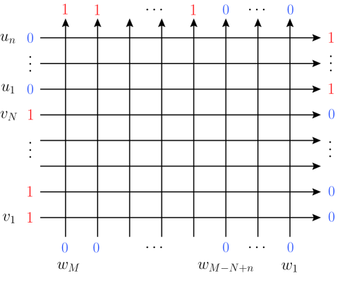
Figure 3: The graphical representation of the intermediate scalar products (3.19) with inhomogeneous parameters $w_{M+1-j}$ associated with site $j$.

We have the following lemma regarding the properties of the intermediate scalar product.

Lemma 3.3.

The intermediate scalar product (3.19) $S(\{u\}_{n}|\{v\}_{N}|\{w\})$ satisfies the following properties.

1. $S(\{u\}_{n}|\{v\}_{N}|\{w\})$ is symmetric with respect to the variables $\{w_{1},\dots,w_{M-N+n}\}$.

2. $\prod_{j=M-N+n+1}^{M}(1+\beta u_{n}/w_{j})^{-1}S(\{u\}_{n}|\{v\}_{N}|\{w\})$ is a polynomial of degree $M-N+n-1$ in $u_{n}$.

3. The following recursive relations between the intermediate scalar products hold

   $$S(\{u\}_{n}|\{v\}_{N}|\{w\})|_{u_{n}=\beta^{-1}w_{M-N+n}}$$

   $$\qquad\qquad=\prod_{j=1}^{M-N+n-1}\frac{w_{M-N+n}}{\beta w_{j}}\prod_{j=M-N+n+1}^{M}\Bigg{(}1+\frac{w_{M-N+n}}{w_{j}}\Bigg{)}S(\{u\}_{n-1}|\{v\}_{N}|\{w\}).$$ (3.20)

4. The case $n=0$ of the intermediate scalar products has the following form:

   $$S(\{u\}_{0}|\{v\}_{N}|\{w\})=\prod_{j=1}^{N}\frac{2v_{j}}{w_{M-N+j}^{j}}\prod_{1\leq j<k\leq N}(v_{j}+v_{k})\prod_{j=1}^{N}\prod_{k=1}^{M-N}\Bigg{(}1-\frac{\beta v_{j}}{w_{k}}\Bigg{)}.$$ (3.21)

Proof.

Property 1 follows from the $RLL$-relation

$$\widetilde{R}_{jk}(w_{M+1-j}/w_{M+1-k})L_{ak}(u/w_{M+1-k})L_{aj}(u/w_{M+1-j})$$

$$\qquad\qquad=L_{aj}(u/w_{M+1-j})L_{ak}(u/w_{M+1-k})\widetilde{R}_{jk}(w_{M+1-j}/w_{M+1-k})$$ (3.22)

holding in $\operatorname{End}(W_{a}\otimes V_{j}\otimes V_{k}$). Here $\widetilde{R}$ is given by

$$\widetilde{R}(v)=\begin{pmatrix}1&0&0&0\\ 0&\beta(v-1)&v&0\\ 0&1&0&0\\ 0&0&0&v\end{pmatrix},$$ (3.23)

which intertwines the $L$-operators acting on a common auxiliary space (but acting on different quantum spaces). Note the usual $RLL$-relation (3.22) intertwines the $L$-operators acting on a same quantum space but acting on different auxiliary spaces. The above $RLL$-relation (3.22) allows one to construct the monodromy matrix as a product of the $L$-operators acting on the same quantum space (see also Appendix for an example of using its property to examine the symmetries of the domain wall boundary partition function), and rewriting the intermediate scalar products in terms of the resultant monodromy matrices makes one see Property 1 holds.

Property 2 can be shown by inserting the completeness relation into the intermediate scalar products

$$S(\{u\}_{n}|\{v\}_{N}|\{w\}) =\langle 1^{N-n}0^{M-N+n}|\prod_{j=1}^{n}\mathcal{C}(u_{j},\{w\})\prod_{k=1}^{N}\mathcal{B}(v_{k},\{w\})|\Omega\rangle$$

$$=\sum_{k=1}^{M-N+n}\langle 1^{N-n}0^{M-N+n}|\mathcal{C}(u_{n},\{w\})|1^{N-n}0^{M-N+n-k}10^{k-1}\rangle$$

$$\qquad\times\langle 1^{N-n}0^{M-N+n-k}10^{k-1}|\prod_{j=1}^{n-1}\mathcal{C}(u_{j},\{w\})\prod_{k=1}^{N}\mathcal{B}(v_{k},\{w\})|\Omega\rangle,$$ (3.24)

and noting that the factor containing $u_{n}$ is calculated as

$$\langle 1^{N-n}0^{M-N+n}|\mathcal{C}(u_{n},\{w\})|1^{N-n}0^{M-N+n-k}10^{k-1}\rangle$$

$$\qquad\qquad=\prod_{j=M-N+n+1}^{M}\Bigg{(}1+\frac{\beta u_{n}}{w_{j}}\Bigg{)}\prod_{j=k+1}^{M-N+n}\Bigg{(}1-\frac{\beta u_{n}}{w_{j}}\Bigg{)}\prod_{j=1}^{k-1}\frac{u_{n}}{w_{j}}.$$ (3.25)

Property 3 can be obtained by setting $u_{n}=\beta^{-1}w_{M-N+n}$ in (3.24), or can be directly observed by its graphical representation that the top row is completely frozen.

To show Property 4, we first note by the graphical representation (see figure 4) that

$$S(\{u\}_{0}|\{v\}_{N}|\{w\})=\prod_{j=1}^{N}\prod_{k=1}^{M-N}\Bigg{(}1-\frac{\beta v_{j}}{w_{k}}\Bigg{)}\langle 1^{N}|\prod_{j=1}^{N}\mathcal{B}_{N}(v_{j})|0^{N}\rangle.$$ (3.26)

where

$$\mathcal{B}_{N}(v_{k})={}_{a}\langle 0|\prod_{j=1}^{N}\mathcal{L}_{aj}(v_{k}/w_{M+1-j})|1\rangle_{a}.$$ (3.27)

One can evaluate the domain wall boundary partition function $\langle 1^{N}|\prod_{j=1}^{N}\mathcal{B}_{N}(v_{j})|0^{N}\rangle$ by the standard procedure following the arguments of Izergin-Korepin [26, 27], which is given in Appendix.

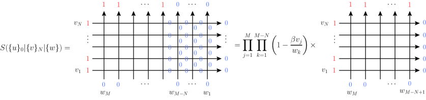
Figure 4: The intermediate scalar products (3.21) for $n=0$, which corresponds to the domain wall boundary partition function.

The result has the following simple factorized form

$$\langle 1^{N}|\prod_{j=1}^{N}\mathcal{B}_{N}(v_{j})|0^{N}\rangle=\prod_{j=1}^{N}\frac{2v_{j}}{w_{M-N+j}^{j}}\prod_{1\leq j<k\leq N}(v_{j}+v_{k}),$$ (3.28)

which together with (3.26) proves Property 4. ∎

Lemma 3.4.

The properties in Lemma 3.3 uniquely determine the intermediate scalar product (3.19).

Due to Lemma 3.4, the following determinant representation for the intermediate scalar product is valid.

Theorem 3.5.

The intermediate scalar product $S(\{u\}_{n}|\{v\}_{N}|\{w\})$ (3.19) has the following determinant form:

$$S(\{u\}_{n}|\{v\}_{N}|\{w\})= \prod_{j=1}^{N}(2v_{j})\prod_{1\leq j<k\leq N}\frac{v_{j}+v_{k}}{v_{k}-v_{j}}\prod_{M-N+n+1\leq j<k\leq M}\frac{1}{\beta(1-w_{k}/w_{j})}$$

$$\times\prod_{1\leq j<k\leq n}\frac{u_{j}+u_{k}}{u_{j}-u_{k}}\mathrm{det}_{N}Q(\{u\}_{n}|\{v\}_{N}|\{w\})$$ (3.29)

with an $N\times N$ matrix $Q(\{u\}_{n}|\{v\}_{N}|\{w\})$ whose matrix elements are given by

$$Q(\{u\}_{n}|\{v\}_{N}|\{w\})_{jk}$$

$$=\begin{cases}\displaystyle\prod_{l=M-N+n+1}^{M}\frac{\displaystyle\beta u_{j}+w_{l}}{\displaystyle\beta u_{j}-w_{l}}\frac{\displaystyle a(u_{j},\{w\})d(v_{k},\{w\})-a(v_{k},\{w\})d(u_{j},\{w\})}{\displaystyle v_{k}-u_{j}},&\text{ ($1\leq j\leq n$)}\\ \displaystyle\frac{1}{w_{M-N+j}}\prod_{\begin{subarray}{c}l=1\\ l\neq M-N+j\end{subarray}}^{M}\left(1-\frac{\beta v_{k}}{w_{l}}\right),&\text{ ($n+1\leq j\leq N$)}\end{cases}.$$ (3.30)

Proof.

We can directly see that the determinant formula (3.29) satisfies all the properties in Lemma 3.3. To show Property 4, we utilize the Cauchy determinant formula

$$\mathrm{det}_{N}\left(\frac{1}{x_{j}-y_{k}}\right)=\frac{\prod_{1\leq j<k\leq N}(x_{k}-x_{j})(y_{j}-y_{k})}{\prod_{j,k=1}^{N}(x_{j}-y_{k})}.$$ (3.31)

Finally due to Lemma 3.4, the determinant formula (3.29) holds. ∎

Corollary 3.6.

Taking $n=N$ in (3.29) yields the determinant representation of the scalar product for the six-vertex model with inhomogeneous parameters (3.16):

$$\langle\Psi(\{u\}_{N},\{w\})| \Psi(\{v\}_{N},\{w\})\rangle$$

$$=\prod_{j=1}^{N}(2v_{j})\prod_{1\leq j<k\leq N}\frac{(u_{j}+u_{k})(v_{j}+v_{k})}{(u_{j}-u_{k})(v_{k}-v_{j})}\mathrm{det}_{N}Q(\{u\}_{N}|\{v\}_{N}|\{w\})$$ (3.32)

with

$$Q(\{u\}_{N}|\{v\}_{N}|\{w\})_{jk}=\frac{a(u_{j},\{w\})d(v_{k},\{w\})-a(v_{k},\{w\})d(u_{j},\{w\})}{v_{k}-u_{j}}.$$ (3.33)

Further taking the homogeneous limit $w_{j}\to 1$ ($1\leq j\leq n$) yields (3.17) in Theorem 3.5.

4 Matrix elements of the $t$-deformed boson model and the six-vertex model

In this section, we derive matrix elements for the $t$-deformed boson model for the generic parameter $t$, and then we restrict ourselves to the case of the six-vertex model $t=-1$.

Consider the arbitrary off-shell state, i.e., the parameters $\{v\}_{N}$ in the $N$-particle state (3.11) are arbitrary. The orthonormal basis of the $N$-particle state $|\Psi(\{v\}_{N})\rangle$ and its dual $\langle\Psi(\{v\}_{N})|$ is given by $|\{n\}_{M,N}\rangle:=|n_{1}\rangle_{1}\ \otimes\dots\otimes|n_{M}\rangle_{M}$ and $\langle\{n\}_{M,N}|:=_{1}\langle n_{1}|\otimes\dots\otimes_{M}\langle n_{M}|$, where $n_{1}+\cdots+n_{M}=N$. The wavefunctions can be expanded in this basis as

$$|\Psi(\{v\}_{N})\rangle=\sum_{\begin{subarray}{c}0\leq n_{1},\dots,n_{M}\leq N\\ n_{1}+\cdots+n_{M}=N\end{subarray}}\langle\{n\}_{M,N}|\psi(\{v\}_{N})\rangle|\{n\}_{M,N}\rangle,$$ (4.1)

$$\langle\Psi(\{v\}_{N})|=\sum_{\begin{subarray}{c}0\leq n_{1},\dots,n_{M}\leq N\\ n_{1}+\cdots+n_{M}=N\end{subarray}}\langle\{n\}_{M,N}|\langle\psi(\{v\}_{N})|\{n\}_{M,N}\rangle.$$ (4.2)

There is a one-to-one correspondence between the set $\{n\}_{M,N}=\{n_{1},\dots,n_{M}\}$ ($n_{1}+\cdots+n_{M}=N$) and the Young diagram $x=(x_{1},x_{2},\dots,x_{N})$ ($M\geq x_{1}\geq x_{2}\geq\cdots\geq x_{N}\geq 1$). Namely, each Young diagram $x$ under the constraint $x_{1}\leq M$, $\ell(x)=N$ can be labeled by a set of integers $\{n\}_{M,N}$ as $x=(M^{n_{M}},\dots,1^{n_{1}})$.

The following definition [23] on the ordering on the basis of particle configurations is useful for later purpose.

Definition 4.1.

[23] For two configurations $\{m\}_{M,N+1}=\{m_{1},\dots,m_{M}\}$ $(m_{1}+\cdots+m_{M}=N+1)$ and $\{n\}_{M,N}=\{n_{1},\dots,n_{M}\}$ $(n_{1}+\cdots+n_{M}=N)$, let $\sum_{j}^{m}=\sum_{k=j}^{M}m_{k}$ and $\sum_{j}^{n}=\sum_{k=j}^{M}n_{k}$. We say that the particle configurations $\{m\}_{M,N+1}$ and $\{n\}_{M,N}$ are admissible, if and only if $0\leq(\sum_{j}^{m}-\sum_{j}^{n})\leq 1$ ($1\leq j\leq M$), and write this relation as $\{m\}_{M,N+1}\triangleright\{n\}_{M,N}$.

Moreover we also define the ordering on the Young diagrams.

Definition 4.2.

For two Young diagrams $y=(y_{1},y_{2},\dots,y_{N+1})$ and $x=(x_{1},x_{2},\dots,x_{N})$, we say that $y$ and $x$ interlace, if and only if $y_{j}\geq x_{j}\geq y_{j+1}$ $(j=1,\dots,N)$, and write this relation as $y\succ x$.

Proposition 4.3.

Let $\{m\}_{M,N+1}$ and $\{n\}_{M,N}$ be the particle configurations described by the Young diagram $y=(y_{1},\dots,y_{N+1})$ and $x=(x_{1},\dots,x_{N})$. Then

$$y\succ x\Longleftrightarrow\{m\}_{M,N+1}\triangleright\{n\}_{M,N}.$$ (4.3)

For $\{m\}_{M,N+1}$ and $\{n\}_{M,N}$, we introduce $\{p\}_{r}=\{1\leq p_{1}<\cdots<p_{r}\leq M\}$ to be the set of all integers $p$ such that $m_{p}=n_{p}+1$, and $\{q\}_{s}=\{1\leq q_{1}<\cdots<q_{s}\leq M\}$ to be the set of all integers $q$ such that $m_{q}+1=n_{q}$. When $\{m\}_{M,N+1}$ and $\{n\}_{M,N}$ satisfy the admissible condition $\{m\}_{M,N+1}\triangleright\{n\}_{M,N}$, $\{p\}_{r}$ and $\{q\}_{s}$ satisfy $s=r-1$ and $p_{k}<q_{k}<p_{k+1}$ ($k=1,\dots,r-1$).

From the matrix elements of the $L$-operator, one finds

$$\langle\{m\}_{M,N+1}|\mathcal{B}(v)|\{n\}_{M,N}\rangle=0,\ \ \ \mathrm{unless}\ \ \ \{m\}_{M,N+1}\triangleright\{n\}_{M,N}.$$ (4.4)

When the admissible condition is satisfied, one finds the following.

$$\langle\{m\}_{M,N+1}|\mathcal{B}(v)|\{n\}_{M,N}\rangle= {}_{a}\langle 0|\langle\{m\}_{M,N+1}|\prod_{j=1}^{M}\mathcal{L}_{aj}(v)|1\rangle_{a}|\{n\}_{M,N}\rangle$$

$$= v^{\sum_{j=1}^{r}p_{j}-\sum_{j=1}^{r-1}q_{j}}\prod_{j=1}^{r}(1-t^{n_{p_{j}}+1})\prod_{j=1}^{r}\prod_{k=p_{j}+1}^{q_{j}-1}(1-\beta vt^{n_{k}}),$$ (4.5)

where $q_{0}=0,\ q_{r}=M+1$.
This can be shown by combining the following partial actions:

$$\prod_{l=q_{j-1}+1}^{q_{j}}\mathcal{L}_{al}(v)|1\rangle_{a}\otimes\left\{\otimes_{k=q_{j-1}+1}^{q_{j}}|n_{k}\rangle_{k}\right\}$$

$$\qquad=v^{p_{j}-q_{j-1}}(1-t^{n_{p_{j}}+1})\prod_{l=p_{j}+1}^{q_{j}-1}(1-\beta vt^{n_{l}})|1\rangle_{a}\left\{\otimes_{k=q_{j-1}+1}^{q_{j}}|m_{k}\rangle_{k}\right\}\quad(1\leq j\leq r-1),$$

$$\prod_{l=q_{r-1}+1}^{M}\mathcal{L}_{al}(v)|1\rangle_{a}\otimes\left\{\otimes_{k=q_{r-1}+1}^{M}|n_{k}\rangle_{k}\right\}$$

$$\qquad=v^{p_{r}-q_{r-1}}(1-t^{n_{p_{r}}+1})\prod_{l=p_{r}+1}^{M}(1-\beta vt^{n_{l}})|0\rangle_{a}\left\{\otimes_{k=q_{r-1}+1}^{M}|m_{k}\rangle_{k}\right\}.$$ (4.6)

Next, we examine the matrix elements of the one-row $B$ and $C$ operators furthermore at the point $t=-1$. We first reduce the matrix elements (4.5) to a simpler form and then translate into the language of Young diagrams. The result for the matrix elements in the language of Young diagrams can be summarized as follows.

Proposition 4.4.

The matrix elements $\langle\{m\}_{M,N+1}|\mathcal{B}(v)|\{n\}_{M,N}\rangle$ at $t=-1$ are given by

$$\langle\{m\}_{M,N+1}|\mathcal{B}(v)|\{n\}_{M,N}\rangle$$

$$\qquad=\frac{1+2\beta z}{(1+\beta z)^{M+1}}\left\{\frac{2(1+\beta z)}{1+2\beta z}\right\}^{\#(y|x)}z^{\sum_{j=1}^{N+1}y_{j}-\sum_{j=1}^{N}x_{j}}\prod_{j=1}^{N}\{1+2\beta z(1-\delta_{x_{j}y_{j+1}})\}.$$ (4.7)

when $x=(x_{1},\dots,x_{N})=(M^{n_{M}},\dots,1^{n_{1}})\subset M^{N}$ and $y=(y_{1},\dots,y_{N+1})=(M^{m_{M}},\dots,1^{m_{1}})\subset M^{N+1}$ are strict partitions satisfying $y\succ x$, and zero otherwise. Here $\#(y|x)$ denotes the number of parts in $y$ which are not in $x$. We regard the product in the right hand side of (4.7) as 1 when $x=\phi$.

Proposition 4.5.

The matrix elements $\langle\{n\}_{M,N}|\mathcal{C}(v)|\{m\}_{M,N+1}\rangle$ at $t=-1$ are given by

$$\langle\{n\}_{M,N}|\mathcal{C}(v)|\{m\}_{M,N+1}\rangle$$

$$= \frac{1}{z(1+\beta z)^{M-1}}\left\{\frac{2(1+\beta z)}{1+2\beta z}\right\}^{\#(y^{\vee}|x^{\vee})-1}z^{\sum_{j=1}^{N+1}y_{j}^{\vee}-\sum_{j=1}^{N}x_{j}^{\vee}}\prod_{j=1}^{N}\{1+2\beta z(1-\delta_{x_{j}^{\vee}y_{j+1}^{\vee}})\}.$$ (4.8)

when $x^{\vee}=(M+1)^{N}/x=(x_{1}^{\vee},\dots,x_{N}^{\vee})=(M^{n_{1}},\dots,1^{n_{M}})\subset M^{N}$ and $y^{\vee}=(M+1)^{N+1}/y=(y_{1}^{\vee},\dots,y_{N+1}^{\vee})=(M^{m_{1}},\dots,1^{m_{M}})\subset M^{N+1}$ are strict partitions satisfying $y^{\vee}\succ x^{\vee}$, and zero otherwise. We regard the product in the right hand side of (4.8) as 1 when $x^{\vee}=\phi$.

Proof.

We show (4.7). Eq. (4.8) can be calculated in the same way.

First, we note that since $\prod_{j=1}^{r}(1-t^{n_{p_{j}}+1})\neq 0$ unless $n_{p_{j}}=1\ (\mathrm{mod}\ 2)$ for all $j$, we only need to consider the case when both $\{m\}_{M,N+1}$ and $\{n\}_{M,N}$ are sequences of numbers 0 and 1. Otherwise, the matrix elements vanish as explained in section 2. Translating this restriction to the language of Young diagrams, this means that we restrict both the partitions $y$ and $x$ to be strict.

The matrix elements for the case $y\succ x$ is calculated as (4.5) for generic $t$, which can be furthermore simplified at $t=-1$ as follows

$$\langle\{m\}_{M,N+1}|\mathcal{B}(v)|\{n\}_{M,N}\rangle= 2^{r}v^{\sum_{j=1}^{r}p_{j}-\sum_{j=1}^{r-1}q_{j}}(1-\beta v)^{\#\{k\in\cup_{j=1}^{r}\{p_{j}+1,\dots,q_{j}-1\}|n_{k}=0\}}$$

$$\times(1+\beta v)^{\#\{k\in\cup_{j=1}^{r}\{p_{j}+1,\dots,q_{j}-1\}|n_{k}=1\}},$$ (4.9)

where $\{m\}_{M,N+1}$ and $\{n\}_{M,N}$ are both sequences of 0 and 1 satisfying $\{m\}_{M,N+1}\triangleright\{n\}_{M,N}$.
Using

$$(1-\beta v)^{\#\{k\in\cup_{j=1}^{r}\{p_{j}+1,\dots,q_{j}-1\}|n_{k}=0\}}$$

$$\qquad\qquad=(1-\beta v)^{\#\{k\in\cup_{j=1}^{r}\{p_{j}+1,\dots,q_{j}-1\}\}}(1-\beta v)^{-\#\{k\in\cup_{j=1}^{r}\{p_{j}+1,\dots,q_{j}-1\}|n_{k}=1\}}$$

$$\qquad\qquad=(1-\beta v)^{\sum_{j=1}^{r-1}q_{j}-\sum_{j=1}^{r}p_{j}+M+1-r-\#\{k\in\cup_{j=1}^{r}\{p_{j}+1,\dots,q_{j}-1\}|n_{k}=1\}},$$ (4.10)

one has

$$\langle\{m\}_{M,N+1}|\mathcal{B}(v)| \{n\}_{M,N}\rangle$$

$$= 2^{r}v^{\sum_{j=1}^{r}p_{j}-\sum_{j=1}^{r-1}q_{j}}(1-\beta v)^{\sum_{j=1}^{r-1}q_{j}-\sum_{j=1}^{r}p_{j}+M+1-r}$$

$$\times\left(\frac{1+\beta v}{1-\beta v}\right)^{\#\{k\in\cup_{j=1}^{r}\{p_{j}+1,\dots,q_{j}-1\}|n_{k}=1\}}$$

$$= 2^{r}(1-\beta v)^{M+1-r}(v^{-1}-\beta)^{\sum_{j=1}^{r-1}q_{j}-\sum_{j=1}^{r}p_{j}}$$

$$\times\left(\frac{1+\beta v}{1-\beta v}\right)^{\#\{k\in\cup_{j=1}^{r}\{p_{j}+1,\dots,q_{j}-1\}|n_{k}=1\}}.$$ (4.11)

From the translation rule [14]

$$\sum_{j=1}^{r}p_{j}-\sum_{j=1}^{r-1}q_{j}=\sum_{j=1}^{N+1}y_{j}-\sum_{j=1}^{N}x_{j},$$

$$r-1+\#\{k\in\cup_{j=1}^{r}\{p_{j}+1,\dots,q_{j}-1\}|n_{k}\neq 0\}=\#\{j\in\{1,\dots,N\}|x_{j}\neq y_{j+1}\},$$ (4.12)

One gets

$$\langle\{m\}_{M,N+1}| \mathcal{B}(v)|\{n\}_{M,N}\rangle$$

$$= 2^{r}(1-\beta v)^{M-r+1}(v^{-1}-\beta)^{\sum_{j=1}^{N}x_{j}-\sum_{j=1}^{N+1}y_{j}}\left(\frac{1+\beta v}{1-\beta v}\right)^{\#\{j\in\{1,\dots,N\}|x_{j}\neq\mu_{j+1}\}-r+1}$$

$$= 2^{r}\left(\frac{1+\beta v}{1-\beta v}\right)^{1-r}(1-\beta v)^{M+1-r}(v^{-1}-\beta)^{\sum_{j=1}^{N}x_{j}-\sum_{j=1}^{N+1}y_{j}}$$

$$\times\prod_{j=1}^{N}\left\{1+\frac{2\beta v}{1-\beta v}(1-\delta_{x_{j},y_{j+1}})\right\}.$$ (4.13)

Introducing the variable $z=(v^{-1}-\beta)^{-1}$ and changing the variable from $v$ to $z$, the matrix elements can be rewritten as

$$\langle\{m\}_{M,N+1}|\mathcal{B}(v)|\{n\}_{M,N}\rangle$$

$$\qquad=2^{r}(1+2\beta z)^{1-r}(1+\beta z)^{r-M-1}z^{\sum_{j=1}^{N+1}y_{j}-\sum_{j=1}^{N}x_{j}}\prod_{j=1}^{N}\{1+2\beta z(1-\delta_{x_{j},y_{j+1}})\},$$ (4.14)

where $r=:\#(y|x)$ is the number of parts in $y$ which are not in $x$. ∎

Note that the elements of the $L$-operator $\mathcal{L}_{aj}(v)$ (2.5)–(2.8) at $t=-1$ reduces to those for the six-vertex model (2.14):

$$\mathcal{L}_{aj}(v)=\begin{pmatrix}1-\beta v&0&0&0\\ 0&1+\beta v&2v&0\\ 0&1&v&0\\ 0&0&0&v\end{pmatrix}_{aj}=\begin{pmatrix}\frac{1}{1+\beta z}&0&0&0\\ 0&\frac{1+2\beta z}{1+\beta z}&\frac{2z}{1+\beta z}&0\\ 0&1&\frac{z}{1+\beta z}&0\\ 0&0&0&\frac{z}{1+\beta z}\end{pmatrix}_{aj}.$$ (4.15)

Example 4.6.

We set $M=5$ and $N=2$ and consider the case $\{m\}_{M,N+1}=\{10011\}$ and $\{n\}_{M,N}=\{00110\}$. Translating into the language of Young diagrams, we have $y=(5,4,1)$ and $x=(4,3)$. One finds $\#(y|x)=2$ since 5 and 1 are in $y$ but not in $x$. We also have $\sum_{j=1}^{3}y_{j}-\sum_{j=1}^{2}x_{j}=3$ and $x_{1}=y_{2}$, $x_{2}\neq y_{3}$. The right hand side of (4.7) becomes $2^{2}z^{3}(1+\beta z)^{-4}$ which can be easily checked to match with the left hand side.

For $\beta=0$, the matrix elements reduce to the skew Schur $Q$-polynomials [24, 25]

$$\langle\{m\}_{M,N+1}|\mathcal{B}(v)|\{n\}_{M,N}\rangle=2^{\#(y|x)}z^{\sum_{j=1}^{N+1}y_{j}-\sum_{j=1}^{N}x_{j}}=Q_{y/x}(z),$$ (4.16)

which we will use to derive the wavefunction in the next section.

5 Wavefunctions of the six-vertex model

Let us examine the wavefunction at the point $t=-1$ where the $t$-boson model reduces to the six-vertex model. We show the corresponding wavefunction is essentially the Schur polynomials.

Definition 5.1.

The Schur polynomial is defined to be the following determinant:

$$s_{\lambda}(\boldsymbol{z})=\frac{\mathrm{det}_{N}(z_{j}^{\lambda_{k}+N-k})}{\prod_{1\leq j<k\leq N}(z_{j}-z_{k})},$$ (5.1)

where $z=\{z_{1},\dots,z_{N}\}$ is a set of variables and $\lambda$ denotes a Young diagram $\lambda=(\lambda_{1},\lambda_{2},\dots,\lambda_{N})$ with weakly decreasing non-negative integers $\lambda_{1}\geq\lambda_{2}\geq\cdots\geq\lambda_{N}\geq 0$.

We show the following equivalence between the wavefunction of the six-vertex model and the Schur polynomials.

Theorem 5.2.

The wavefunction has the following form

$$\langle\{m\}_{M,N}|\prod_{j=1}^{N}\mathcal{B}(v_{j})|\Omega\rangle=\frac{2^{N}\prod_{j=1}^{N}z_{j}\prod_{1\leq j<k\leq N}(z_{j}+z_{k}+2\beta z_{j}z_{k})}{\prod_{j=1}^{N}(1+\beta z_{j})^{M}}s_{\lambda}(\boldsymbol{z}).$$ (5.2)

where $z_{j}=(v_{j}^{-1}-\beta)^{-1}$ and $\lambda=(\lambda_{1},\dots,\lambda_{N})\subset(M-N)^{N}$ is a partition related to $x=(x_{1},\dots,x_{N})=(M^{m_{M}},\dots,1^{m_{1}})$ by $\lambda_{j}=x_{j}-N+j-1$.

The dual wavefunction has the following form

$$\langle\Omega|\prod_{j=1}^{N}\mathcal{C}(v_{j})|\{m\}_{M,N}\rangle=\frac{\prod_{1\leq j<k\leq N}(z_{j}+z_{k}+2\beta z_{j}z_{k})}{\prod_{j=1}^{N}(1+\beta z_{j})^{M-1}}s_{\lambda^{\vee}}(\boldsymbol{z}),$$ (5.3)

where $\lambda^{\vee}$ is the Poincare dual of $\lambda$: $\lambda^{\vee}=(\lambda_{1}^{\vee},\dots,\lambda_{N}^{\vee}),\ \lambda_{j}^{\vee}=M-N-\lambda_{N+1-j}$.

We remark that the integrable model we consider here seems to be a special case of the one considered in [12], whose wavefunction was obtained by the coordinate Bethe ansatz up to a normalization factor. However, to prove combinatorial formulae, it is crucial to determine the exact form starting from the first principle, i.e., starting from the $L$-operator, since we combine the above theorem with the exact expression for the matrix elements (4.7) and (4.8) derived in the previous section to derive a new combinatorial formula for example.

Proof.

We show (5.2). Eq. (5.3) can be proved in the same way. First, we redefine the $L$-operator as

$$\widetilde{\mathcal{L}}_{aj}(z)=(1+\beta z)\mathcal{L}_{aj}(v)=\begin{pmatrix}1&0&0&0\\ 0&1+2\beta z&2z&0\\ 0&1+\beta z&z&0\\ 0&0&0&z\end{pmatrix}_{aj},$$ (5.4)

and the corresponding monodromy matrix

$$\widetilde{\mathcal{T}}_{a}(z)=\prod_{j=1}^{M}\widetilde{\mathcal{L}}_{aj}(z)=\begin{pmatrix}\widetilde{\mathcal{A}}(z)&\widetilde{\mathcal{B}}(z)\\ \widetilde{\mathcal{C}}(z)&\widetilde{\mathcal{D}}(z)\end{pmatrix}_{a},$$ (5.5)

and show the following equivalent equality for (5.2)

$$\langle\{m\}_{M,N}|\prod_{j=1}^{N}\widetilde{\mathcal{B}}(z_{j})|\Omega\rangle=2^{N}\prod_{j=1}^{N}z_{j}\prod_{1\leq j<k\leq N}(z_{j}+z_{k}+2\beta z_{j}z_{k})s_{\lambda}(\boldsymbol{z}).$$ (5.6)

To prove this, we first show the following lemma

Lemma 5.3.

$$\frac{\langle\{m\}_{M,N}|\prod_{j=1}^{N}\widetilde{\mathcal{B}}(z_{j})|\Omega\rangle}{\prod_{1\leq j<k\leq N}(z_{j}+z_{k}+2\beta z_{j}z_{k})},$$ (5.7)

does not depend on $\beta$.

Proof.

We prove this lemma by showing the following properties for $\langle\{m\}_{M,N}|\prod_{j=1}^{N}\widetilde{\mathcal{B}}(z_{j})|\Omega\rangle$:

1. $\langle\{m\}_{M,N}|\prod_{j=1}^{N}\widetilde{\mathcal{B}}(z_{j})|\Omega\rangle$ is a polynomial of $\beta$ with highest degree $N(N-1)/2$.

2. $\langle\{m\}_{M,N}|\prod_{j=1}^{N}\widetilde{\mathcal{B}}(z_{j})|\Omega\rangle$ has $z_{j}+z_{k}+2\beta z_{j}z_{k}$, $1\leq j<k\leq N$ as factors.

We first show $\mathrm{deg}_{\beta}\langle\{m\}_{M,N}|\prod_{j=1}^{N}\widetilde{\mathcal{B}}(z_{j})|\Omega\rangle\leq N(N-1)/2$ by induction on $N$. The case $N=1$ follows as an special case of the general fact $\mathrm{deg}_{\beta}\langle\{m\}_{M,{N+1}}|\widetilde{\mathcal{B}}(z)|\{n\}_{M,N}\rangle\leq N$ which can be seen easily from the definition of the $L$-operator $\widetilde{\mathcal{L}}(z)$. Next, let us assume $\mathrm{deg}_{\beta}\langle\{m\}_{M,N}|\prod_{j=1}^{N}\widetilde{\mathcal{B}}(z_{j})|\Omega\rangle\leq N(N-1)/2$. One can see $\mathrm{deg}_{\beta}\langle\{m\}_{M,N+1}|\prod_{j=1}^{N+1}\widetilde{\mathcal{B}}(z_{j})|\Omega\rangle\leq(N+1)N/2$ by combining the assumption $\mathrm{deg}_{\beta}\langle\{m\}_{M,N}|\prod_{j=1}^{N}\widetilde{\mathcal{B}}(z_{j})|\Omega\rangle\leq N(N-1)/2$, the fact $\mathrm{deg}_{\beta}\langle\{m\}_{M,{N+1}}|\widetilde{\mathcal{B}}(z)|\{n\}_{M,N}\rangle\leq N$ and the decomposition

$$\langle\{m\}_{M,N+1}|\prod_{j=1}^{N+1}\widetilde{\mathcal{B}}(z_{j})|\Omega\rangle=\sum_{\{n\}_{M,N}}\langle\{m\}_{M,{N+1}}|\widetilde{\mathcal{B}}(z_{N+1})|\{n\}_{M,N}\rangle\langle\{n\}_{M,N}|\prod_{j=1}^{N}\widetilde{\mathcal{B}}(z_{j})|\Omega\rangle.$$ (5.8)

Next, we show Property 2. It is enough to show the case $N=2$. The case for generic $N$ follows from the commutativity ${[}\widetilde{\mathcal{B}}(z_{j}),\widetilde{\mathcal{B}}(z_{k}){]}=0$ and the decomposition

$$\langle\{m\}_{M,N}|\prod_{j=1}^{N}\widetilde{\mathcal{B}}(z_{j})|\Omega\rangle=\sum_{\{n\}_{M,2}}\langle\{m\}_{M,N}|\prod_{j=3}^{N}\widetilde{\mathcal{B}}(z_{j})|\{n\}_{M,2}\rangle\langle\{n\}_{M,2}|\widetilde{\mathcal{B}}(z_{1})\widetilde{\mathcal{B}}(z_{2})|\Omega\rangle.$$ (5.9)

Now we show for the case $N=2$ by induction on $M$. Let us denote the $A,B,C,D$ operators consisting of $M$ $L$-operators as $\widetilde{\mathcal{B}}_{M}(z)$ for example. The case $M=2$ can be checked explicitly $\langle 1,1|\widetilde{\mathcal{B}}_{M}(z_{1})\widetilde{\mathcal{B}}_{M}(z_{2})|\Omega\rangle=4z_{1}z_{2}(z_{1}+z_{2}+2\beta z_{1}z_{2})$ . Let us assume that $\langle x_{1},x_{2}|\widetilde{\mathcal{B}}_{M}(z_{1})\widetilde{\mathcal{B}}_{M}(z_{2})|\Omega\rangle$ has $z_{1}+z_{2}+2\beta z_{1}z_{2}$ as a factor. We examine $\langle x_{1},x_{2}|\widetilde{\mathcal{B}}_{M+1}(z_{1})\widetilde{\mathcal{B}}_{M+1}(z_{2})|\Omega\rangle$. One can easily show by its graphical description that

$$\langle x_{1},x_{2}|\widetilde{\mathcal{B}}_{M+1}(z_{1})\widetilde{\mathcal{B}}_{M+1}(z_{2})|\Omega\rangle=(z_{1}z_{2})^{x_{1}-1}\langle x_{1},x_{2}|\widetilde{\mathcal{B}}_{x_{2}-x_{1}+1}(z_{1})\widetilde{\mathcal{B}}_{x_{2}-x_{1}+1}(z_{2})|\Omega\rangle.$$ (5.10)

If $x_{1}\neq 1$ or $x_{2}\neq M+1$, $\langle x_{1},x_{2}|\widetilde{\mathcal{B}}_{M+1}(z_{1})\widetilde{\mathcal{B}}_{M+1}(z_{2})|\Omega\rangle$ has $z_{1}+z_{2}+2\beta z_{1}z_{2}$ as a factor by assumption.

We examine the remaining case $x_{1}=1,x_{M+1}=M+1$. We show

$$\langle 1,M+1|\widetilde{\mathcal{B}}_{M+1}(z_{1})\widetilde{\mathcal{B}}_{M+1}(z_{2})|\Omega\rangle=4z_{1}z_{2}\frac{z_{1}^{M}-z_{2}^{M}}{z_{1}-z_{2}}(z_{1}+z_{2}+2\beta z_{1}z_{2}).$$ (5.11)

By graphical description, one sees

$$\langle x_{1},x_{2}|\widetilde{\mathcal{B}}_{M+1}(z_{1})\widetilde{\mathcal{B}}_{M+1}(z_{2})|\Omega\rangle=2z_{1}\{f_{M}(z_{1},z_{2})+2z_{2}^{M+1}(1+2\beta z_{1})\},$$ (5.12)

where $f_{M}(z_{1},z_{2})=\langle 1|\widetilde{\mathcal{D}}_{M}(z_{1})\widetilde{\mathcal{B}}_{M}(z_{2})|\Omega\rangle$. Again, we use its graphical representation to derive the following recursive relation

$$f_{M}(z_{1},z_{2})=z_{1}\{f_{M-1}(z_{1},z_{2})+4z_{2}^{M}(1+\beta z_{1})\},$$ (5.13)

with the initial condition

$$f_{2}(z_{1},z_{2})=2z_{1}z_{2}(z_{1}+2z_{2}+2\beta z_{1}z_{2}).$$ (5.14)

We can show by induction that

$$f_{M}(z_{1},z_{2})=2z_{2}\frac{z_{1}^{M}-z_{2}^{M}}{z_{1}-z_{2}}(z_{1}+z_{2}+2\beta z_{1}z_{2})-2z_{2}^{M+1}(1+2\beta z_{1}),$$ (5.15)

solves the recursive relation (5.13) and the initial condition (5.14). Hence, the expression (5.11) follows from (5.12) and (5.15). We thus have shown by induction that
$\langle x_{1},x_{2}|\widetilde{\mathcal{B}}_{M+1}(z_{1})\widetilde{\mathcal{B}}_{M+1}(z_{2})|\Omega\rangle$ has $z_{1}+z_{2}+2\beta z_{1}z_{2}$ as a factor, and Property 2 is proved.

From Property 2 we have, $\mathrm{deg}_{\beta}\langle\{m\}_{M,N}|\prod_{j=1}^{N}\widetilde{\mathcal{B}}(z_{j})|\Omega\rangle\geq N(N-1)/2$. Together with
$\mathrm{deg}_{\beta}\langle\{m\}_{M,N}|\prod_{j=1}^{N}\widetilde{\mathcal{B}}(z_{j})|\Omega\rangle\leq N(N-1)/2$ which we proved before, we have Property 1. ∎

From Lemma 5.3, one can examine

$$\frac{\langle\{m\}_{M,N}|\prod_{j=1}^{N}\widetilde{\mathcal{B}}(z_{j})|\Omega\rangle}{\prod_{1\leq j<k\leq N}(z_{j}+z_{k}+2\beta z_{j}z_{k})},$$ (5.16)

by dealing the case $\beta=0$.

Lemma 5.4.

We have

$$\left.\frac{\langle\{m\}_{M,N}|\prod_{j=1}^{N}\widetilde{\mathcal{B}}(z_{j})|\Omega\rangle}{\prod_{1\leq j<k\leq N}(z_{j}+z_{k}+2\beta z_{j}z_{k})}\right|_{\beta=0}=2^{N}\prod_{j=1}^{N}z_{j}s_{\lambda}(\{\boldsymbol{z}\}).$$ (5.17)

Proof.

To prove the lemma is equivalent to show

$$\langle\{m\}_{M,N}|\prod_{j=1}^{N}\widetilde{\mathcal{B}}(z_{j})|\Omega\rangle|_{\beta=0}=2^{N}\prod_{j=1}^{N}z_{j}\prod_{1\leq j<k\leq N}(z_{j}+z_{k})s_{\lambda}({\boldsymbol{z}})=Q_{x}({\boldsymbol{z}}).$$ (5.18)

where $Q_{x}({\boldsymbol{z}})$ is the Schur $Q$-function

$$Q_{x}(\boldsymbol{z})=2^{N}\sum_{w\in S_{N}}w\left(\prod_{j=1}^{N}z_{j}^{x_{j}}\prod_{1\leq j<k\leq N}\frac{z_{j}+z_{k}}{z_{j}-z_{k}}\right),$$ (5.19)

where $\boldsymbol{z}=\{z_{1},\dots,z_{N}\}$ is a set of variables and $x$ denotes a strict Young diagram $x=(x_{1},x_{2},\dots,x_{N})$ with strictly decreasing non-negative integers $x_{1}>x_{2}>\cdots>x_{N}\geq 0$. (5.18) follows from the fact (4.16) derived in the previous section that the matrix element of a single $B$-operator at $\beta=0$ is nothing but the skew Schur $Q$-function

$$\langle\{m\}_{M,N+1}|\widetilde{\mathcal{B}}(z)|\{n\}_{M,N}\rangle|_{\beta=0} =\langle\{m\}_{M,N+1}|\mathcal{B}(v)|\{n\}_{M,N}\rangle|_{\beta=0}$$

$$=2^{\#(y|x)}z^{\sum_{j=1}^{N+1}y_{j}-\sum_{j=1}^{N}x_{j}}$$

$$=Q_{y/x}(z).$$ (5.20)

(5.18) follows as a consequence of the addition formula for the skew Schur $Q$-function

$$\langle\{m\}_{M,N+2}| \widetilde{\mathcal{B}}(z_{1})\widetilde{\mathcal{B}}(z_{2})|\{n\}_{M,N}\rangle|_{\beta=0}$$

$$=\sum_{\ell}\langle\{m\}_{M,N+2}|\widetilde{\mathcal{B}}(z_{1})|\{\ell\}_{M,N+1}\rangle|_{\beta=0}\langle\{\ell\}_{M,N+1}|\widetilde{\mathcal{B}}(z_{2})|\{n\}_{M,N}\rangle|_{\beta=0}$$

$$=\sum_{w}Q_{y/w}(z_{1})Q_{w/x}(z_{2})$$

$$=Q_{y/x}(z_{1},z_{2}).$$ (5.21)

∎

Combining Lemma 5.3 and (5.17), we have (5.6), and the proof of (5.2) is completed. ∎

6 Combinatorial formulae for the Schur polynomials

By combining the analysis of the partition functions in the previous sections, we obtain combinatorial formulae for the Schur polynomials.

Theorem 6.1.

We have the following combinatorial formula for the Schur polynomials

$$s_{\lambda}(\boldsymbol{z})= \frac{1}{\prod_{1\leq j<k\leq N}(z_{j}+z_{k}+2\beta z_{j}z_{k})}\sum_{x^{(N)}\succ x^{(N-1)}\succ\dots\succ x^{(0)}=\phi}\prod_{k=1}^{N}\Bigg{\{}z_{k}^{\sum_{j=1}^{k}x_{j}^{(k)}-\sum_{j=1}^{k-1}x_{j}^{(k-1)}-1}$$

$$\times \left(\frac{2(1+\beta z_{k})}{1+2\beta z_{k}}\right)^{\#(x^{(k)}|x^{(k-1)})-1}\prod_{j=1}^{k-1}\left(1+2\beta z_{k}(1-\delta_{x_{j}^{(k-1)}x_{j+1}^{(k)}})\right)\Bigg{\}},$$ (6.1)

where $\beta$ is an arbitrary parameter. $x^{(k)}=(x_{1}^{(k)},\dots,x_{k}^{(k)})$, $k=0,1,\dots,N$ are strict partitions satisfying the interlacing relations $x^{(N)}\succ x^{(N-1)}\succ\dots\succ x^{(0)}=\phi$, and $x^{(N)}$ is fixed by the Young diagram $\lambda=(\lambda_{1},\dots,\lambda_{N})$ as $\lambda_{j}=x_{j}^{(N)}-N+j-1$.

Proof.

We decompose the wavefunction as

$$\langle\{n\}_{M,N}|\Psi(\{v\}_{N})\rangle$$

$$\quad=\sum_{\{m^{(0)}\},\dots,\{m^{(N-1)}\}}\langle\{n\}_{M,N}|\prod_{j=1}^{N}\left\{\mathcal{B}(v_{j})|\{m^{(N-j)}\}_{M,N-j}\rangle\langle\{m^{(N-j)}\}_{M,N-j}|\right\}|\Omega\rangle.$$ (6.2)

We insert the expression (5.2) in the left hand side of (6.2) on one hand. On the other hand, the right hand side of (6.2) can be expressed using the evaluation of matrix elements (4.7). Combining the two expressions and simplifying gives the combinatorial expression for the Schur polynomials (6.1). ∎

Example 6.2.

Let us check the case $N=2$, $\lambda=(1,0)$. $x^{(2)}$ is fixed as $x^{(2)}=(1,0)+(2,1)=(3,1)$ and $x^{(0)}=\phi$. $x^{(1)}$ satisfying the interlacing relation $x^{(2)}\succ x^{(1)}\succ x^{(0)}$ has three cases $x^{(1)}=(1)$, $x^{(1)}=(2)$ and $x^{(1)}=(3)$. Each term in the sum of the right hand side of (6.1) has the contribution

$$z_{2}^{4-1-1}\left(\frac{2(1+\beta z_{2})}{1+2\beta z_{2}}\right)^{1-1}z_{1}^{1-1},$$ (6.3)

$$z_{2}^{4-2-1}\left(\frac{2(1+\beta z_{2})}{1+2\beta z_{2}}\right)^{2-1}(1+2\beta z_{2})z_{1}^{2-1},$$ (6.4)

$$z_{2}^{4-3-1}\left(\frac{2(1+\beta z_{2})}{1+2\beta z_{2}}\right)^{1-1}(1+2\beta z_{2})z_{1}^{3-1},$$ (6.5)

which sums up to $(z_{1}+z_{2}+2\beta z_{1}z_{2})(z_{1}+z_{2})$. Dividing by $z_{1}+z_{2}+2\beta z_{1}z_{2}$, we have $z_{1}+z_{2}$, which is nothing but $s_{(1,0)}(z_{1},z_{2})$.

Proposition 6.3.

The following well-known identity holds true for the Schur polynomials.

$$\sum_{\lambda\subseteq(M-N)^{N}}s_{\lambda}(\boldsymbol{z})s_{\lambda^{\vee}}(\boldsymbol{y})=\prod_{1\leq j<k\leq N}\frac{1}{(z_{k}-z_{j})(y_{j}-y_{k})}\mathrm{det}_{N}\left[\frac{z_{j}^{M}-y_{j}^{M}}{z_{j}-y_{k}}\right].$$ (6.6)

Proof.

First, substituting the completeness relation, one decomposes the scalar product as

$$\langle\Psi(\{u\}_{N})|\Psi(\{v\}_{N})\rangle=\sum_{\{n\}_{M,N}}\langle\Psi(\{u\}_{N})|\{n\}_{M,N}\rangle\langle\{n\}_{M,N}|\Psi(\{v\}_{N})\rangle.$$ (6.7)

Then substituting the determinant representation for the scalar product (3.17) into the RHS of the above and utilizing the relations (5.2) and (5.3) yields the Cauchy identity (6.6) by changing the variables from $u_{j}$ and $v_{j}$ to $y_{j}=(u_{j}^{-1}-\beta)^{-1}$ and $z_{j}=(v_{j}^{-1}-\beta)^{-1}$ respectively. ∎

7 Enumeration of alternating sign matrices

In this section, we make an application of the domain wall boundary partition function to the enumeration of alternating sign matrices. See [30, 31, 32, 33, 34, 35, 36, 37, 38, 39] for example of a huge literature on the relation between the enumeration of alternating sign matrices and integrable vertex models. The presentation below for the explanation of the relation between alternating sign matrices and the six-vertex model follows the lines of [38]. We take the homogeneous limit of the domain wall boundary partition function (3.28) or (A.1)

$$Z(\{v\}_{n}|\{1\})=\langle 1^{n}|\prod_{k=1}^{n}\mathcal{B}(v_{k})|\Omega\rangle=\prod_{j=1}^{n}(2v_{j})\prod_{1\leq j<k\leq n}(v_{j}+v_{k}).$$ (7.1)

An algebraic analytic proof of (3.28) is given in Appendix. It can also be obtained as a special case of the wavefunction (5.2).

As a corollary of the domain wall boundary partition function, we derive a simple expression for a special case of the generating function of alternating sign matrices.

Definition 7.1.

Alternating sign matrices are square matrices with the following properties:

1. each entry is either 0, 1 or $-1$.

2. there is at least one nonzero entry in each row and column.

3. the entries in each row and column sum to 1.

To satisfy the above conditions, the nonzero entries must alternate in sign along each row and column.

Example 7.2.

For $n=3$, there are 7 alternating sign matrices:

$$\mathrm{ASM}(3) =\left\{\begin{pmatrix}1&0&0\\ 0&1&0\\ 0&0&1\end{pmatrix},\begin{pmatrix}0&0&1\\ 0&1&0\\ 1&0&0\end{pmatrix},\begin{pmatrix}1&0&0\\ 0&0&1\\ 0&1&0\end{pmatrix},\right.$$

$$\qquad\qquad\left.\begin{pmatrix}0&0&1\\ 1&0&0\\ 0&1&0\end{pmatrix},\begin{pmatrix}0&1&0\\ 1&0&0\\ 0&0&1\end{pmatrix},\begin{pmatrix}0&1&0\\ 0&0&1\\ 1&0&0\end{pmatrix},\begin{pmatrix}0&1&0\\ 1&-1&1\\ 0&1&0\end{pmatrix}\right\}.$$ (7.2)

Definition 7.3.

Let $\mathrm{ASM}(n)$ be the set consisting of all $n\times n$ alternating sign matrices. For $A\in\mathrm{ASM}(n)$, let us define

$$\nu(A):=\sum_{\begin{subarray}{c}1\leq i<k\leq n\\ 1\leq\ell\leq j\leq n\end{subarray}}A_{ij}A_{k\ell},$$ (7.3)

$\mu(A)$ as the number of $-1$’s in $A$ and $\rho(A)$ as the number of 0’s to left of 1 in the first row of $A$. The generating function of the alternating sign matrices is defined as

$$Z_{\mathrm{ASM}}(n,x,y,z)=\sum_{A\in\mathrm{ASM}(n)}x^{\nu(A)}y^{\mu(A)}z^{\rho(A)}.$$ (7.4)

Each element of an alternating sign matrix $\mathrm{ASM}(n)$ has one-to-one correspondence with a particular configuration which makes a non-zero contribution to the domain wall boundary partition function of the six-vertex model. To simplify the explanation, we identify a particular configuration of the domain wall boundary partition function at the coordinate $(j,k)$ with the matrix elements ${}_{a}\langle*|{}_{j}\langle*|\mathcal{L}_{aj}(v_{k})|*\rangle_{a}|*\rangle_{j}$.

Definition 7.4.

Let $\mathrm{6VDW}(n)$ be the set of all particular configurations making non-zero contributions to the domain wall boundary partition function of the six-vertex model. For $C\in\mathrm{6VDW}(n)$, Let $\nu(C)$ be the number of vertex configurations ${}_{a}\langle 1|{}_{j}\langle 1|\mathcal{L}_{aj}(v_{k})|1\rangle_{a}|1\rangle_{j}$, $j,k=1,\dots,n$ in $C$, $\mu(C)$ the number of vertex configurations ${}_{a}\langle 1|{}_{j}\langle 0|\mathcal{L}_{aj}(v_{k})|0\rangle_{a}|1\rangle_{j}$, $j,k=1,\dots,n$ in $C$, $\rho(C)$ the number of vertex configurations ${}_{a}\langle 1|{}_{j}\langle 1|\mathcal{L}_{aj}(v_{n})|1\rangle_{a}|1\rangle_{j}$, $j=1,\dots,n$ in $C$.

Theorem 7.5.

[40] There is a bijection between the set of alternating sign matrices $\{A\in\mathrm{ASM}(n)\ |\ \nu(A)=p,\mu(A)=m,\rho(A)=k\}$ and the set of configurations making non-zero contributions to the domain wall boundary partition function of the six-vertex model $\{C\in\mathrm{6VDW}(n)\ |\ \nu(C)=p,\mu(C)=m,\rho(C)=k\}$ by identifying the matrix elements 1 with ${}_{a}\langle 0|{}_{j}\langle 1|\mathcal{L}_{aj}(v_{k})|1\rangle_{a}|0\rangle_{j}$, $-1$ with ${}_{a}\langle 1|{}_{j}\langle 0|\mathcal{L}_{aj}(v_{k})|0\rangle_{a}|1\rangle_{j}$ and 0 with one of the rest of the four non-zero configurations.

Proposition 7.6.

[40] Let $\#{}_{a}\langle*|{}_{j}\langle*|\mathcal{L}_{aj}(v_{k})|*\rangle_{a}|*\rangle_{j}$ be the number of vertex configurations
${}_{a}\langle*|{}_{j}\langle*|\mathcal{L}_{aj}(v_{k})|*\rangle_{a}|*\rangle_{j}$, $j,k=1,\dots,n$ in a configuration $C\in\mathrm{6VDW}(n)$.

$$\#{}_{a}\langle 0|{}_{j}\langle 0|\mathcal{L}_{aj}(v_{k})|0\rangle_{a}|0\rangle_{j} =\nu(C),$$ (7.5)

$$\#{}_{a}\langle 0|{}_{j}\langle 1|\mathcal{L}_{aj}(v_{k})|0\rangle_{a}|1\rangle_{j} =n(n-1)/2-\nu(C)-\mu(C),$$ (7.6)

$$\#{}_{a}\langle 0|{}_{j}\langle 1|\mathcal{L}_{aj}(v_{k})|1\rangle_{a}|0\rangle_{j} =\mu(C)+n,$$ (7.7)

$$\#{}_{a}\langle 1|{}_{j}\langle 0|\mathcal{L}_{aj}(v_{k})|0\rangle_{a}|1\rangle_{j} =\mu(C),$$ (7.8)

$$\#{}_{a}\langle 1|{}_{j}\langle 0|\mathcal{L}_{aj}(v_{k})|1\rangle_{a}|0\rangle_{j} =n(n-1)/2-\nu(C)-\mu(C),$$ (7.9)

$$\#{}_{a}\langle 1|{}_{j}\langle 1|\mathcal{L}_{aj}(v_{k})|1\rangle_{a}|1\rangle_{j} =\nu(C).$$ (7.10)

We use (7.1), Theorem 7.5 and Proposition 7.6 to show the following simple formula for a particular type of the generating function of alternating sign matrices:

Proposition 7.7.

$$Z_{\mathrm{ASM}}(n,u-1,u,1)=u^{n(n-1)/2}.$$ (7.11)

Proof.

We first take the homogeneous limit $v_{j}\to v$, $j=1,\dots,n$ of the partition function of the six-vertex model (7.1):

$$Z(v):=Z(\{v\}_{n}|\{1\})|_{v_{1},\dots,v_{n}\to v}=(2v)^{n(n+1)/2}.$$ (7.12)

On the other hand, by the definition of domain wall boundary partition function and Proposition 7.6, we have

$$Z(v)=\sum_{C\in\mathrm{6VDW}(n)}(a_{0}a_{1})^{\nu(C)}(b_{0}b_{1})^{n(n-1)/2-\nu(C)-\mu(C)}c_{0}^{\mu(C)}c_{1}^{\mu(C)+n},$$ (7.13)

where $a_{0}=1-\beta v$, $a_{1}=v$, $b_{0}=1+\beta v$, $b_{1}=v$, $c_{0}=1$, $c_{1}=2v$.
Combining (7.12) and (7.13) and simplifying, one gets

$$\sum_{C\in\mathrm{6VDW}(n)}\left(\frac{1-\beta v}{1+\beta v}\right)^{\nu(C)}\left(\frac{2}{1+\beta v}\right)^{\mu(C)}=\left(\frac{2}{1+\beta v}\right)^{n(n-1)/2}.$$ (7.14)

We make change variable from $v$ to $u:=2/(1+\beta v)$. Finally, we use Theorem 7.5 on the one-to-one correspondence between the set of alternating sign matrices and the set of configurations of the domain wall boundary partition function to replace the sum over $C\in\mathrm{6VDW}(n)$ and the numbers $\nu(C)$, $\mu(C)$ by the sum over $A\in\mathrm{ASM}(n)$ and the numbers $\nu(A)$, $\mu(A)$. Then (7.14) can be rewritten as (7.11), which concludes the proof. ∎

Example 7.8.

For $n=3$, there are 7 alternating sign matrices as in (7.2). Summing up all the corresponding factors, we have $Z_{\mathrm{ASM}}(3,u-1,u,1)=(u-1)^{3}+2(u-1)^{2}+(u-1)u+2(u-1)+1=u^{3}.$

We finally remark that it may also be possible to derive (7.11) as a limit of the determinant representation for $Z_{\mathrm{ASM}}(M,x,y,1)$ in [38].

8 Conclusion

In this paper, we derived a new combinatorial formula for the Schur polynomials. The quantum integrability is useful to derive a formula even for Schur polynomials which is the most fundamental symmetric polynomials. The formula expresses Schur polynomials with an additional parameter besides the spectral parameter. The other known formula in a similar sense is the Tokuyama formula, which can be interpreted as a deformation of the Weyl character formula and the determinant expression. The representation theoretic meaning of the deformation parameter in our formula is unknown now which may be worth investigating. There may be other possibilities to find combinatorial formulae to express Schur polynomials and other symmetric polynomials in terms of additional parameters using the power of quantum integrability. This may be achieved by dealing with partition functions consisting of different local $L$-operators or changing global boundary conditions for example.

Besides the traditional problem of the application of partition functions of the six-vertex model to the enumeration of alternating sign matrices, one of the most active line of researches on quantum integrable combinatorics today is to derive combinatorial formulae for symmetric polynomials such as the Cauchy identity, Littlewood identity and so on by analyzing the transfer matrices or partition functions of integrable lattice models. The power of quantum integrable combinatorics is that one can fuse combinatorics with algebraic analysis to find and prove identities which seems to be hard to show in a purely combinatorial or a purely algebraic way. See [5, 6, 29, 41, 42] for finite lattice and [43] for infinite lattice for example of the recent progresses on this line.

Appendix A Evaluation of the domain wall boundary partition function

Here we derive the factorized form (3.28) of the domain wall boundary partition function defined by

$$Z(\{v\}_{N}|\{w\}_{N}):=\langle 1^{N}|\prod_{j=1}^{N}\mathcal{B}_{N}(v_{j})|0^{N}\rangle,$$ (A.1)

where $\mathcal{B}_{N}(v_{j})$ is given by (3.27) and $\{w\}_{N}=\{w_{M+1-N},\cdots,w_{M}\}$.

Proposition A.1.

The domain wall boundary partition function (A.1) is expressed as the following factorized form:

$$Z(\{v\}_{N}|\{w\}_{N})=\prod_{j=1}^{N}\frac{2v_{j}}{w_{j}^{j}}\prod_{1\leq j<k\leq N}(v_{j}+v_{k}).$$ (A.2)

Proof.

This can be shown in the standard approach due to Izergin and Korepin [26, 27]. First, one shows the following four conditions.

Lemma A.2.

The domain wall boundary partition function (A.1) satisfies the following properties.

1. $\prod_{j=M+1-N}^{M}w_{j}^{N+j-M}Z(\{v\}_{N}|\{w\}_{N})$ is symmetric with respect to the variables $\{w\}_{N}$.

2. $Z(\{v\}_{N}|\{w\}_{N})/v_{N}$ is a polynomial of degree $N-1$ in $v_{N}$.

3. The following recursive relations between the domain wall boundary partition functions hold:

   $$Z( \{v\}_{N}|\{w\}_{N})|_{v_{N}=\beta^{-1}w_{M-N+1}}$$

   $$=-\frac{2}{\beta}\prod_{j=M-N+2}^{M}\left(-\frac{w_{M-N+1}}{\beta w_{j}}\right)\prod_{j=1}^{N-1}\left(1-\frac{\beta v_{j}}{w_{M-N+1}}\right)Z(\{v\}_{N-1}|\{w\}_{N-1}).$$ (A.3)

4. The case $N=1$ of the domain wall boundary partition function following form:

   $$Z(\{v\}_{1}|\{w\}_{1})=\frac{2v_{1}}{w_{M}}.$$ (A.4)

Properties 2, 3 and 4 can be shown easily with the help of the graphical representation (see figure 5 for Property 3) of the domain wall boundary partition function Let us explain Property 1.

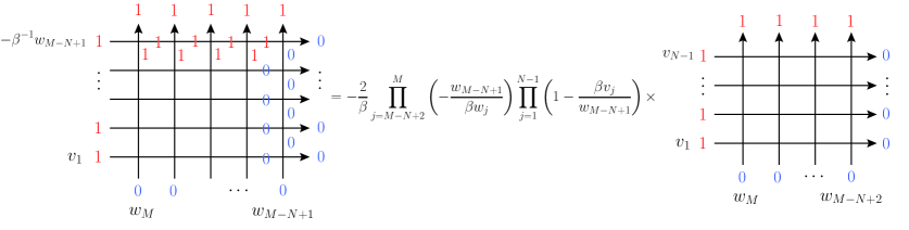
Figure 5: A graphical description of (A.3).

First note that the domain wall boundary partition function $Z(\{v\}_{N}|\{w\}_{N})$ can be re-expressed using the transfer matrix $T_{j}(w_{M+1-j})=\prod_{a=1}^{N}\mathcal{L}_{aj}(v_{a}/w_{M+1-j})\in\operatorname{End}(W^{\otimes N}\otimes\mathcal{F}_{j})$ propagating in the horizontal direction as

$$Z(\{v\}_{N}|\{w\}_{N})={}_{a}\langle 1^{N}|C(w_{M+1-N})\cdots C(w_{M})|0^{N}\rangle{}_{a},$$ (A.5)

where

$$T_{j}(w_{M+1-j}) =\begin{pmatrix}A(w_{M+1-j})&B(w_{M+1-j})\\ C(w_{M+1-j})&D(w_{M+1-j})\end{pmatrix}_{j},$$ (A.6)

From the $RLL$ relation, one has

$$C(w_{k})w_{j}C(w_{j})=C(w_{j})w_{k}C(w_{k}).$$ (A.7)

Combining (A.5) and (A.7) shows Property 1.

The remaining thing to do is to find the explicit forms of the functions satisfying the properties in the Lemma. One can easily show that

$$Z(\{v\}_{N}|\{w\}_{N})=\prod_{j=1}^{N}(2v_{j})\prod_{j=M+1-N}^{M}w_{j}^{M-N-j}\prod_{1\leq j<k\leq N}(v_{j}+v_{k}),$$ (A.8)

satisfies the above four properties. ∎

References

- [1] A. Okounkov and N. Reshetikhin, Correlation function of Schur process with application to local geometry of a random 3-dimensional Young diagram, J. Amer. Math. Soc. 16 (2003) 581-603. [arXiv:math/0107056v3]
- [2] T. Tokuyama, A generating function of strict Gelfand patterns and some formulas on characters of general linear groups, J. Math. Soc. Japan 40 (1988) 671-685.
- [3] S. Okada, Alternating sign matrices and some deformations of Weyl’s denominator formula, J. Algebraic Comb. 2 (1993) 155-176.
- [4] A. M. Hamel and R. C. King, Bijective proofs of shifted tableau and alternating sign matrix identities, J. Algebraic Combin. 25 (2007) 417-458. [arXiv:math/0507479]
- [5] B. Brubaker, D. Bump and S. Friedberg, Schur polynomials and the Yang-Baxter equation, Commun. Math. Phys. 308 (2011) 281-301. [arXiv:0912.0911v3]
- [6] D. Bump, P. McNamara and M. Nakasuji, Factorial Schur functions and the Yang-Baxter equation, Comm. Math. Univ. St. Pauli 63 (2014) 23-45. [arXiv:1108.3087]
- [7] S. J. Tabony, Deformations of characters, metaplectic Whittaker functions and the Yang-Baxter equation, PhD. Thesis, Massachusetts Institute of Technology, USA, 2011.
- [8] B. Brubaker, D. Bump, G. Chinta and P.E. Gunnells, Metaplectic functions and crystals od type B, in Multiple Dirichlet Series, L-Functions, and Automorphic Forms, D. Bump, S. Friedberg and D. Goldfield, eds., Progress in Math. 300 (2012) Birkhauser Boston, 93-118.
- [9] B. Brubaker and A. Schultz, Deformations of the Weyl character formula for classical groups and the six-vertex model. [arXiv:1402.2339v2]
- [10] A. M. Hamel and R. C. King, Half-turn symmetric alternating sign matrices and Tokuyama type factorisation for orthogonal group characters. [arXiv:1402.6773v1]
- [11] T. Sasamoto and M. Wadati, Exact results for one-dimensional totally asymmetric diffusion models, J. Phys. A: Math. Gen. 31 (1998) 6057-6071.
- [12] Y. Takeyama, A discrete analogue of periodic delta Bose gas and affine Hecke algebra, Funckeilaj Ekvacioj 57 (2014) 107-118. [arXiv:1209.2758]
- [13] N. M. Bogoliubov and M. Nassar, On the spectrum of the non-Hermitian phase difference model, Phys. Lett. A 234 (1997) 345-350.
- [14] K. Motegi and K. Sakai, -theoretic boson-fermion correspondence and melting crystals, J. Phys. A: Math. Theor. 47 (2014) 445202. [arXiv:1311.6076]
- [15] A. Lascoux and M. Schutzenberger Structure de Hopf de lanneau de cohomologie et de lanneau de Grothendieck dune variete de drapeaux, C. R. Acad. Sci. Paris Ser. I Math. 295 (1982) 629-633.
- [16] S. Fomin and A. N. Kirillov, Grothendieck polynomials and the Yang-Baxter equation, Proc. 6th Int. Conf. on Formal Power Series and Algebraic Combinatorics (DIMACS) (1994) pp 183-190.
- [17] A. Buch, A Littlewood-Richardson rule for the K-theory of Grassmannians, Acta Math. 189 (2002) 37-78. [arXiv:math/0004137]
- [18] T. Ikeda and H. Naruse, K-theoretic analogues of factorial Schur P- and Q-functions, Adv. Math. 243 (2013) 22-66. [arXiv:1112.5223]
- [19] A. N. Kirillov and H. Naruse, Construction of double Grothendieck polynomials of classical types using Id-Coxeter algebras. [arXiv:1504.08089]
- [20] N. M. Bogoliubov, Boxed plane partitions as an exactly solvable boson model, J. Phys. A: Math. Gen. 38 9415-9430.
- [21] K. Shigechi and M. Uchiyama, Boxed skew plane partition and integrable phase model, J. Phys. A: Math. Gen. 38 10287-10306. [arXiv:cond-mat/0508090]
- [22] C. Korff and C. Stroppel, The sl(n)-WZNW Fusion Ring: a combinatorial construction and a realisation as quotient of quantum cohomology, Adv. Math. 225 (2010) 200-268, [arXiv:0909.2347]
- [23] M. Wheeler, Free fermions in classical and quantum integrable models, PhD thesis, Department of Mathematics and Statistics, University of Melbourne. [arXiv:1110.6703v1]
- [24] N.V. Tsilevich, Quantum Inverse Scattering Method for the -Boson Model and Symmetric functions, Funct. Anal. Appl. 40 (2006) 207-217. [arXiv:math-ph/0510073v1]
- [25] C. Korff, Cylindric versions of specialised Macdonald functions and a deformed Verlinde algebra, Commun. Math. Phys. 318 (2013) 173-246. [arXiv:1110.6356v3]
- [26] V. E. Korepin, Calculation of Norms of Bethe Wave Functions, Commun. Math. Phys. 86 (1982) 391-418.
- [27] A. G. Izergin, Partition Function of the 6-Vertex Model in a Finite Volume, Sov. Phys. Dokl. 32 (1987) 878.
- [28] M. Wheeler, An Izergin-Korepin procedure for calculating scalar products in the six-vertex model, Nucl. Phys. B 852 (2011) 468. [arXiv:1104.2113]
- [29] K. Motegi and K. Sakai, Vertex models, TASEP and Grothendieck polynomials, J. Phys. A: Math. Theor. 46 (2013) 355201. [arXiv:1305.3030]
- [30] D. Bressoud, Proofs and confirmations: The story of the alternating sign matrix conjecture, MAA Spectrum, Mathematical Association of America, Washington, DC, 1999.
- [31] G. Kuperberg, Another proof of the alternating-sign matrix conjecture, Int. Math. Res. Not. 3 (1996) 139-150. [arXiv:math/9712207]
- [32] G. Kuperberg, Symmetry classes of alternating-ssign matrices under one roof, Ann. Math. 156 (2002) 835-866. [arXiv:math/0008184]
- [33] S. Okada, Enumeration of symmetry classes of alternating sign matrices and characters of classical groups, J. Alg. Comb. 23 (2001) 43-69. [arXiv:math/0408234]
- [34] F. Colomo and A. G. Pronko, Square ice, alternating sign matrices and classical orthogonal polynomials, J. Stat. Mech. (2005) P01005. [arXiv:math-ph/0411076]
- [35] F. Colomo and A. G. Pronko, The role of orthogonal polynomials in the six-vertex model and its combinatorial applications, J. Phys. A: Math. Gen. 39 (2006) 9015-9033. [arXiv:math-ph/0602033]
- [36] P. Biane, L. Cantini and A. Sportiello, Doubly-refined enumeration of alternating sign matrices and determinants of 2-staircase Schur functions, Séminaire Lotharingien de Combinatorie, B 65f (2012). [arXiv:1101.3427]
- [37] A. Ayyer and D. Romnik, New enumeration formulas for alternating sign matrices and square ice partition functions, Adv. Math. 235 (2013) 161-186. [arXiv:1202.3651]
- [38] R. Behrend, P. Di Francesco and P. Zinn-Justin, On the weighted enumeration of alternating sign matrices and descending plane paritions, J. Combin. Theory Ser. A 119 (2012) 331-363. [arXiv:1103.1176]
- [39] R. Behrend, Multiply-refined enumeration of alternating sign matrices, Adv. Math. 245 (2013) 439-499. [arXiv:1203.3187]
- [40] N. Elkies, G. Kuperberg, M. Larsen and J. Propp, Alternating sign matrices and domino tilings, J. Alg. Comb. 1 (1992) 111-132, 219-234. [arXiv:math/9201305]
- [41] D. Betea and M. Wheeler, Refined Cauchy and Littlewood identities, plane partitions and symmetry classes of alternating sign matrices, [arXiv:1402.0229]
- [42] D. Betea, M. Wheeler and P. Zinn-Justin, Refined Cauchy/Littlewood identities and six-vertex model partition functions: II. Proofs and new conjectures, [arXiv:1405.7035]
- [43] A. Borodin, On a family of symmetric rational functions, [arXiv:1410.0976]