Low Mach Number Modeling of Convection in Helium Shells on Sub-Chandrasekhar White Dwarfs II:
Bulk Properties of Simple Models

Abstract

The dynamics of helium shell convection driven by nuclear burning establish the conditions for runaway in the sub-Chandrasekhar mass, double detonation model for Type Ia supernovae, as well as for a variety of other explosive phenomena. We explore these convection dynamics for a range of white dwarf core and helium shell masses in three dimensions using the low Mach number hydrodynamics code Maestro. We present calculations of the bulk properties of this evolution, including time-series evolution of global diagnostics, lateral averages of the 3D state, and the global 3D state. We find a variety of outcomes including quasi-equilibrium, localized runaway, and convective runaway. Our results suggest the double detonation progenitor model is promising and that 3D, dynamic convection plays a key role.

1 Introduction

Despite being rather inert embers of evolved stars on their own, white dwarfs (WDs) manage to be at the center of many of the Universe’s most spectacular explosions through interactions with companion stars. One of the most recently proposed manifestations of such an explosion are “.Ia” events (Bildsten et al., 2007), with the decimal point meant to indicate the events are about a tenth the brightness for a tenth the time of type Ia supernovae (SNe Ia).

The proposed .Ia progenitor consists of a carbon/oxygen (C/O) WD accreting from a helium-rich companion. A prominent example of such a system are AM Canum Venaticorum (AM CVn) binaries (Warner, 1995; Nelemans, 2005). In their Letter, Bildsten et al. (2007) calculate that under the right conditions the thermonuclear timescale in an AM CVn’s helium envelope can approach the dynamical timescale, possibly establishing conditions for a detonation which consumes the envelope but leaves the WD core intact. This yields a relatively faint transient a tenth the brightness of a normal SNe Ia. A unique aspect of these calculations is the unprecedentedly low ignition pressures, which is related to the unprecedentedly low masses of the helium envelopes considered. Previous work considering similar systems in the context of double detonations, in which the helium detonation triggers a detonation of the WD core, assumed higher shell masses (Nomoto, 1982a; Woosley et al., 1986; Livne, 1990; Livne & Glasner, 1990, 1991; Woosley & Weaver, 1994; García-Senz et al., 1999), excepting a data point in Nomoto (1982b) and artificial detonations in Livne & Arnett (1995).

As suggested by the authors of the Letter, many took on the task of a detailed reexamination of these systems with lower mass helium shells. A particularly broad and detailed reexamination was carried out by Woosley & Kasen (2011). As they demonstrate, sub-Chandrasekhar mass (sub-M_Ch ) C/O WDs with low-mass helium shells can yield a variety of explosive phenomena, including helium novae, double detonations, and deflagrations that consumed the envelope, leaving behind a hot core. The potential to produce such a variety of transient events motivates extensive theoretical inquiry, especially as we approach first light for the Large Synoptic Survey Telescope (Ivezic et al., 2008). A great deal of this inquiry has been carried out, with tantalizing results.

Much of the focus has been on these systems as double detonation SNe Ia progenitors. Detonation of the C/O core appears to be very robustly triggered by compression waves if detonation occurs in the helium shell (Fink et al., 2007, 2010; Woosley & Kasen, 2011; Shen & Bildsten, 2014), even in the case of asynchronous, asymmetric ignition points (Moll & Woosley, 2013). This makes sub-M_Ch promising candidates as SNe Ia progenitors. Thin helium shells have been shown to be capable of carrying sustained detonations, and may even contribute to features found in SNe Ia observations (Townsley et al., 2012). Synthetic spectra and light curves indicate that if the C/O core detonates and dominates over helium shell effects in the observables, many sub-M_Ch progenitor systems are promising candidates for normal SNe Ia (Sim et al., 2010; Woosley & Kasen, 2011; Fink et al., 2010; Kromer et al., 2010). In particular, work to date favors C/O cores that are near 1.0 $M_{\odot}$ and hot if they are to produce normal SNe Ia. The core-only (no He shell) explosions of Sim et al. (2010) agree best with normal SNe Ia properties for C/O WDs near 1.0 $M_{\odot}$. The 1D models and subsequent synthetic observables of Woosley & Kasen (2011) agree best with normal SNe Ia’s for their “hot” models in which the core relaxed to a luminosity of $1.0~{}L_{\odot}$ as compared to their “cool” models, relaxing to $0.01~{}L_{\odot}$ before helium accretion was modeled.

Further, delay time distribution calculations based on binary population synthesis find distributions and rates for sub-M_Ch SNe Ia progenitor models consistent with being at least one plausible dominant channel for reproducing distributions and rates based on observations (Ruiter et al., 2011). Similar calculations focusing on a subset of sub-M_Ch progenitors find they may be the progenitors of SNe Iax (Wang et al. (2013), though see also Liu et al. (2015b, a)). Geier et al. (2013) present observational evidence for both a helium-accreting sub-M_Ch progenitor system and a high velocity helium-rich star that matches the expected properties of the unbound companion star following a sub-M_Ch SNe Ia. Brown et al. (2011) analyze a sample of WD binary systems including extremely low mass WDs in the context of AM CVn binaries and sub-luminous SNe Ia. They calculate merger rates that are comparable to the observed rates of sub-luminous SNe Ia. Drout et al. (2013) compare observations of SN 2005ek with many possible models, including sub-M_Ch systems. In particular they argue that if SN 2005ek did have a sub-M_Ch progenitor, an edge-lit detonation would be the most viable model. In the edge-lit scenario, the detonation in the helium layer propagates directly into the core, setting off a carbon detonation at the core/shell interface.

We caution that theoretical studies (and the study reported here) have limits and make many assumptions. The importance of realistic compositions and convective mixing have been made clear (Kromer et al., 2010; Shen & Moore, 2014; Piro, 2015). In addition we note that it is currently computationally impossible in any model of the full core/shell system to fully resolve ignition of core detonation, which occurs on 0.01 – 1 cm scales for densities $\rho=10^{7}$–$10^{8}~{}\mathrm{g~{}cm^{-3}}$. Instead, such work must report the critical conditions achieved in a given computational cell or group of cells and argue the likelihood of them achieving ignition of detonation. This challenge is in part addressed in Shen & Bildsten (2014), who carry out small-scale, fully resolved calculations of detonation ignition in regimes relevant to the C/O core of sub-M_Ch systems. They argue that conditions reported in multi-dimensional studies of the full core/shell system are sufficient for ignition in many cases, though lower mass (roughly, below 0.8 $M_{\odot}$) or O/Ne cores are less likely to experience ignition.

A significant uncertainty remains. Only one-dimensional (1D) models have demonstrated development of a detonation in these lower mass helium shells. Multi-dimensional work has focused on assuming ignition of detonation and exploring the consequences. In this series of papers, we hope to begin to fill this gap by modeling the development of ignition and elucidating the detailed 3D properties of the system leading up to and at the moment of such an ignition. The first paper in the series details our methodology, carries out numerical experiments, and demonstrates the development of a localized runaway in a model with a 1.0 $M_{\odot}$ core and 0.05 $M_{\odot}$ shell (Zingale et al. (2013), hereafter Paper I). In this paper we apply our methodology to a large number of models at higher resolution, carry out a new numerical experiment, and include many new analyses and diagnostics. The purpose of this paper is to

• expand our methodology to a much larger suite of models,

• explore what broad outcomes and trends we find for simple initial models, and to

• characterize the bulk properties of these models, including global 3D structure, 1D averages of the 3D state, and peak global properties such as the properties of the hottest cell in the domain.

This broad exploration lays a foundation for more targeted analysis of a smaller number of more sophisticated models.

We defer a detailed analysis of potential ignition in these simple models, including the geometry, timing, number, and statistics of localized igniting volumes, to the next paper in this series. We also want to be clear that one cost of doing such a broad study is that we must use simple models motivated by detailed 1D models. Our methodology also fundamentally limits us from modeling the development of a detonation. Instead, we are modeling the dynamics we expect immediately prior (a few convective turnover times) to any ignition. Thus, we model the development of potential seeds of a detonation or deflagration. The ultimate fate of these seeds should be the focus of future work.

To begin, we describe our models and methodology.

2 Methodology and Models

Our simulations are performed using Maestro, a finite-volume, adaptive mesh stellar hydrodynamics code suitable for flows where the fluid speed is much less than the sound speed. Maestro models the flow using a low Mach number approximation—sound waves are filtered out of the system, but compressibility effects due to stratification and local heat release are retained. While the code is mature and has been used in state-of-the-art astrophysical modeling, it is also under active development. Nonaka et al. (2010) is the most recent and comprehensive in a series of papers describing the low Mach number equation set and numerical algorithm. The simulations reported here make use of an improved low Mach number equation set; this and the associated algorithmic changes relative to the model used in Nonaka et al. (2010) are described in Appendix A. The Maestro source code, including all the code needed to run the models reported here, and User’s Guide are available in the public release. Please see these for the full details of the most current form of the algorithm.

Paper I lays out in detail our numerical strategy for modeling sub-M_Ch WDs with helium shells and demonstrates the robustness of results to parameter variation. Below we review the methodology and describe the configuration of the suite of models used to broadly sample the explosive regimes of sub-M_Ch systems.

2.1 Microphysics

We utilize a general, publicly available stellar equation of state (Timmes & Swesty, 2000; Timmes, 2008). Ions, radiation, degenerate and relativistic electrons, and Coulomb corrections are all incorporated.

Our nuclear reaction network is quite simple for the sake of computational efficiency, enabling a broad sampling of parameter space (see §2.5). It is important to note that Woosley & Kasen (2011) emphasize two crucial reactions for exploring sub-M_Ch systems: ${}^{14}\rm{N}(e^{-},\nu)^{14}\rm{C}(\alpha,\gamma)^{18}\rm{O}$ (NCO) and ¹²C(p, $\gamma$)¹³N($\alpha$,p)¹⁶O (CagO-bypass). Additionally, Shen & Bildsten (2009) demonstrate the importance of ${}^{14}\rm{N}(\alpha,\gamma)^{18}\rm{F}$ (NagF). While we agree these reactions are crucial to understanding sub-M_Ch models, we can neglect them for the purposes of exploring the dominant energetics in the pre-ignition burning. For more on our rationale for neglecting them and the conditions under which they can be neglected, see Appendix B. We employ a simple network consisting of the isotopes ¹²C, ⁴He, and ¹⁶O and the rates for 3 ${}^{4}\rm{He}\rightarrow^{12}$C (triple-alpha) and ¹²C($\alpha$,$\gamma$)¹⁶O (CagO). CagO is included because it can allow for the tracing of ${}^{16}\rm{O}$ production which in turn traces the sites of vigorous burning and how polluted the shell becomes with burning products.

Our baseline reaction rates come from Caughlan & Fowler (1988), with screening as in Graboske et al. (1973); Weaver et al. (1978); Alastuey & Jancovici (1978); Itoh et al. (1979). The CagO reaction rate is scaled by a factor of 1.7, as recommended in Weaver & Woosley (1993); Garnett (1997). Thermodynamic derivatives are held constant over a single timestep as described in Almgren et al. (2008).

2.2 Initial Models

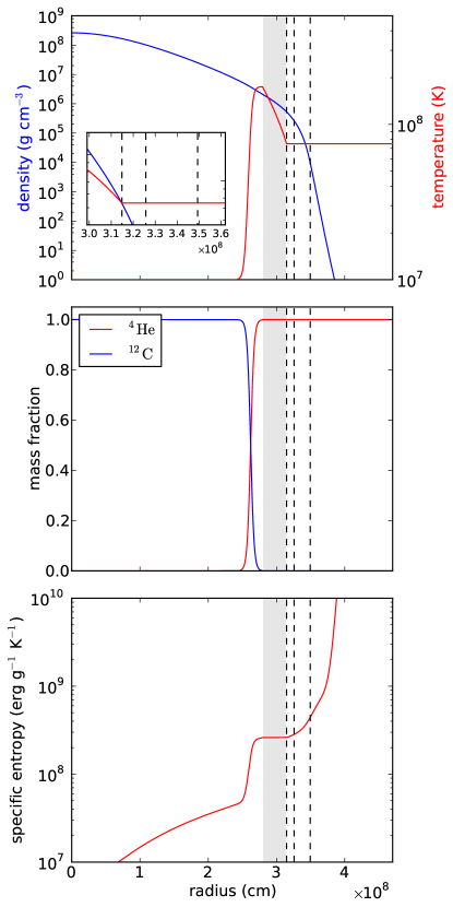
Maestro evolves both a 1D hydrostatic base state and a 3D hydrodynamic state. For spherical problems, such as the sub-M_Ch system, this base state is radial. To set the initial conditions for our 3D problem we initialize the base state and map that state onto the 3D grid. Our sub-M_Ch initial models are defined by four parameters: the mass of the WD core, $M_{\mathrm{WD}}$, the isentropic helium shell’s mass, $M_{\mathrm{He}}$, the temperature at the base of the helium shell, $T_{\mathrm{base}}$, and the core’s isothermal temperature, $T_{\mathrm{core}}$. At the interface between the core and the shell there is a sharp composition and temperature gradient following the prescription described in §2.2 of Paper I. We generate our own initial models using an iterative scheme that enforces hydrostatic equilibrium and the values of $T_{\mathrm{core}}$ and $T_{\mathrm{base}}$ while converging on the given ($M_{\mathrm{WD}}$, $M_{\mathrm{He}}$). Figure 1 demonstrates a representative initial model.

Figure 1: A representative initial model with $M_{\mathrm{WD}}$ = 1.2 $M_{\odot}$, $M_{\mathrm{He}}$ = 0.05 $M_{\odot}$, $T_{\mathrm{core}}=10^{7}$ K, $T_{\mathrm{base}}=1.75\times 10^{8}$ K. The shaded region is the convection zone. The dashed lines from left to right are: the start of the sponge, the anelastic cutoff, and the base cutoff density (see §2.4). Top: Temperature (red) and density (blue) profiles. The inset zooms in on the sponge and cutoff radii. Middle: Mass fraction profiles of carbon (blue) and helium (red). Bottom: Specific entropy profile.

We expand upon Paper I by adding a new parameter test. Most initial models for the simulations reported here use the same transition width parameter $\delta$ as in Paper I: $\delta=50~{}\mathrm{km}$. However, we carried out a supplemental suite of simulations for model 11030 (see §2.5) in which all parameters are the same save for a $\delta$ one-fourth, one-half, and twice the original magnitude of 50 km. The quadrupled resolution on a side in this paper allows us to resolve sharper transitions than in Paper I. Recall that this tanh-smoothing is necessary for the problem to be well-posed. A sharp discontinuity in grid-based hydrodynamics makes it impossible to demonstrate convergence as it offers no resolvable solution to converge to (see Paper I for convergence tests). The 50 km value for $\delta$ in the lower resolution models of Paper I provided roughly 10 cells of radial resolution over which to resolve the transition. The lowest $\delta$ examined in this paper, 12.5 km, offers similar resolution of the transition. In addition, it is not well-known exactly how transitions from core to shell are realized in nature. Thus, this parameter study has both a numerical and physical motivation.

The top row of Fig. 11 demonstrates the transition for 11030d0.25 (one-fourth the original $\delta$) and the reference model 11030. See § 3.5 for discussion of results.

2.3 Grid Structure

The 3D grid is Cartesian. For all models except one (see §2.5) an octant of the sub-M_Ch WD is modeled, allowing us to capture 3D effects yet achieve much greater computational efficiency and explore a large number of models. The impact of simulating an octant instead of the full star is investigated in Paper I. As we discuss in §3.1, the higher resolutions and larger model set presented here introduce complications at the boundaries for octant runs with localized runaway.

The grid is adaptively refined to focus resolution and computational power on the regions of greatest interest. To study the dynamics of the convection and nuclear burning in the helium shell, we refine zones in which $\mathrm{X}_{\mathrm{He}}>0.01$ at a density greater than $\rho_{\mathrm{cutoff}}$ (see §2.4). To better resolve the shells, in this study we further refine cells with temperatures $T>125$ MK. We are satisfied with two levels of refinement for models with a $0.8~{}M_{\odot}$ core. The mass-radius relationship for WDs means these models will have the largest radius and consequently the thickest shells spatially. However, for models having $M_{\mathrm{core}}\geq 1.0~{}M_{\odot}$ the spatial extent of the shell is greatly reduced, which is exacerbated by the fact that more massive cores have lower mass helium shells. Thus, for all such models we add an extra level of refinement for a total of four levels (the base grid, which we label level one, and three additional, further refined levels).

Figure 2: A representative slice of the initial grid for $M_{\mathrm{WD}}$ = 1.0 $M_{\odot}$, $M_{\mathrm{He}}$ = 0.04 $M_{\odot}$, $T_{\mathrm{core}}=10^{8}$ K, $T_{\mathrm{base}}=1.85\times 10^{8}$ K. The different colors indicate grid patches at different levels of refinement. Level 1 is the base (coarse) level.

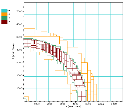
Figure 2 illustrates the grid we have described. This figure outlines grid patches for each of the levels in the initial grid for model 10040H (for details about our adaptive mesh algorithm and the definition of grid patches, see §5 of Nonaka et al. (2010)). At the coarsest (base) level, all octant runs have a 256³ resolution with a refinement factor of 2 between levels, leading to subsequent 512³, 1024³, and 2048³ effective resolutions within the refined patches. We include one full star run (08130F, see §2.5), which has a 512³ coarse (base) resolution. The strong dependence of radius on mass in WDs results in a range of physical resolutions $\Delta x\approx$ 2.5 - 15.8 km at the finest level. The 1D base state’s resolution is not adaptively refined; instead, it has a fixed resolution of five times that of the finest level: 5120 cells. This factor of five is first used and discussed in Zingale et al. (2009).

2.4 Boundaries

The boundary conditions for our simulations are reflecting on the symmetry faces of octant domains (lower x, y, and z), and outflow (zero-gradient) on the other faces. A full star simulation has outflow boundary conditions on all faces of the domain.

As can be seen in Fig. 2, the grid includes a coarsely-resolved region well outside the convective zone. This serves to keep the convective surface insensitive to boundary conditions. A steep drop in density occurs at stellar surfaces (as seen in Fig. 1). Without modification, this rapid decline precipitates a rapid spike in velocity to conserve momentum. The advantages of a low Mach method become negligible if fluid velocities in any zone approach the sound speed. Thus much work has been put into developing strategies to address steep density gradients at stellar surfaces without significantly impacting Maestro’s computational or physical validity. The details of these treatments can be found in Paper I (§2.3), Zingale et al. (2011), and Nonaka et al. (2012).

Briefly, two density cutoffs are implemented: the anelastic cutoff $\rho_{\mathrm{anelastic}}$ and the low-density cutoff $\rho_{\mathrm{cutoff}}$ (see Fig. 1). For zones with densities below $\rho_{\mathrm{anelastic}}$, Maestro switches to an anelastic-like velocity constraint that helps damp velocities (see Almgren et al. (2008)). Density is held constant once it falls to $\rho_{\mathrm{cutoff}}$, halting the steep decline. To prevent impacting validity its value is chosen such that the regions with $\rho\leq\rho_{\mathrm{cutoff}}$ contain an insignificant proportion of the system’s total mass. These cutoffs are supplemented with a numerical sponge that damps surface velocities (Almgren et al., 2008). Cutoff values for all simulations are discussed in §2.5.

This combination of cutoffs, a sponge, and maintaining a buffer zone in the computational domain between the stellar surface and the domain’s boundaries enables us to study surface convection in detail over long timescales without surface effects significantly impacting our results.

Table 1: Model Set

label	($M_{\mathrm{core}},M_{\mathrm{He}}$)	$T_{\mathrm{core}}$	$T_{\mathrm{base}}(t=0)$	$\rho_{\mathrm{base}}$	$x_{\mathrm{max}}$	$\Delta x_{\mathrm{fine}}$	$\rho_{\mathrm{anelastic}}$	$t_{\mathrm{final}}/\langle\tau_{\mathrm{conv}}\rangle$			outcome
	[$M_{\odot}$]	[K]	[$\times 10^{8}$ K]	[$\times 10^{5}~{}\mathrm{g~{}cm^{-3}}$]	[km]	[km]	[$\times 10^{5}~{}\mathrm{g~{}cm^{-3}}$]	min	avg	max
12030H	(1.2, 0.03)	$10^{8}$	1.75	10.1	05300	02.6	$1.29$	02.3	08.8	12.1	l
12030	(1.2, 0.03)	$10^{7}$	1.75	10.8	05100	02.5	$1.37$	01.5	06.4	08.6	l
12020H	(1.2, 0.02)	$10^{8}$	1.75	06.2	05500	02.7	$0.80$	03.1	10.3	17.1	l
12020	(1.2, 0.02)	$10^{7}$	1.75	06.8	05300	02.6	$0.87$	03.0	12.4	19.4	l
11030H	(1.1, 0.03)	$10^{8}$	1.85	05.7	06600	03.2	$0.67$	02.7	10.6	17.5	l
11030d0.25	(1.1, 0.03)	$10^{7}$	1.90	06.0	06400	03.1	$0.68$	12.1	04.7	35.9	l
11030d0.5	(1.1, 0.03)	$10^{7}$	1.90	06.0	06400	03.1	$0.68$	09.8	08.5	29.1	l
11030	(1.1, 0.03)	$10^{7}$	1.90	06.0	06400	03.1	$0.68$	01.9	26.3	13.6	l
11030d2	(1.1, 0.03)	$10^{7}$	1.90	06.0	06400	03.1	$0.68$	02.5	32.6	09.4	l
11020H	(1.1, 0.02)	$10^{8}$	1.85	03.6	06900	03.4	$0.43$	01.5	03.8	09.0	q
11020	(1.1, 0.02)	$10^{7}$	1.85	03.9	06600	03.2	$0.46$	05.2	19.5	27.2	q
10040H	(1.0, 0.04)	$10^{8}$	1.85	05.0	07700	03.8	$0.58$	07.1	23.4	27.6	q
10040	(1.0, 0.04)	$10^{7}$	1.85	05.3	07400	03.6	$0.62$	04.2	14.9	18.4	q
10030H	(1.0, 0.03)	$10^{8}$	1.85	03.5	07900	03.9	$0.42$	01.2	04.6	07.8	q
10030	(1.0, 0.03)	$10^{7}$	1.85	03.8	07600	03.7	$0.45$	01.5	06.5	08.3	q
08130H	(0.8, 0.13)	$10^{8}$	1.85	09.9	08300	08.1	$1.15$	00.6	03.8	08.4	l
08130F	(0.8, 0.13)	$10^{7}$	1.85	10.9	16200	15.8	$1.26$	00.2	01.3	06.3	l
08130	(0.8, 0.13)	$10^{7}$	1.85	10.7	08100	07.9	$1.25$	00.6	04.2	10.4	l
08120H	(0.8, 0.12)	$10^{8}$	1.85	08.8	08500	08.3	$1.03$	01.8	07.7	10.8	l
08120	(0.8, 0.12)	$10^{7}$	1.75	09.6	08100	07.9	$1.22$	08.4	25.7	27.9	l
08050	(0.8, 0.05)	$10^{7}$	2.50	02.6	10100	09.9	$0.19$	00.9	02.7	07.1	c

2.5 Model Set

Maestro’s ability to take large timesteps as well as the nature of sub-M_Ch pre-explosive dynamics make a broad sampling of the parameter space in 3D computationally feasible. What exactly is the parameter space of interest? To determine this we draw on the results of Bildsten et al. (2007) and the many studies they inspired.

The parameters of greatest interest are the core and helium shell mass configurations. The motivating question is how ignition develops and how it is characterized in minimal helium shell mass systems for a range of core masses. Figure 2 of Bildsten et al. (2007) illustrates their determination of the minimum shell masses for which the nuclear burning timescale is on the order of the dynamical timescale for isothermal cores with $T_{\mathrm{core}}=3\times 10^{7}$ K. Such a short nuclear burning timescale suggests the possibility of thermonuclear runaway even for thin helium shells with $M_{\mathrm{He}}\lesssim 0.05$ – $0.0125M_{\mathrm{core}}$ for $1.0$ – $1.2~{}M_{\odot}$ cores. This work is extended and deepened in subsequent studies, which are largely consistent with the essential results of the 2007 work (Shen & Bildsten, 2009; Brooks et al., 2015). Woosley & Kasen (2011) carry out an extensive set of 1D sub-M_Ch calculations and generate an analogous figure (Figure 19). They include the impact of varying $T_{\mathrm{core}}$. For $M_{\mathrm{core}}=0.7~{}M_{\odot}$, runaway can occur with helium shells having $\sim$ 15% of the core’s mass, perhaps not sufficiently thin for SNe Ia-like spectra. As $M_{\mathrm{core}}$ increases to $1.1~{}M_{\odot}$, runaway can be achieved with shells $\sim$ 2.25% of the core’s mass for hotter cores ($T_{\mathrm{core}}\sim 7.5\times 10^{7}$ K), making SNe Ia-like spectra more achievable. The bare (no helium shell) 1D sub-M_Ch WD detonation calculations of Sim et al. (2010) suggest systems with $M_{\mathrm{core}}\gtrsim 1.0~{}M_{\odot}$ can yield observables in reasonable agreement with the range of observed normal SNe Ia while lower $M_{\mathrm{core}}$ systems can produce characteristics of observed sub-luminous SNe Ia. Fink et al. (2010)’s 2D calculations also find they can produce many characteristics of the range of observed SNe Ia and that core detonation is triggered by shell detonations for ($M_{\mathrm{core}},M_{\mathrm{He}}$) = (0.810 – 1.385, 0.126 – 0.0035) $M_{\odot}$.

Given these studies and the uncertainties involved we investigate systems with $M_{\mathrm{core}}=0.8,1.0,1.1,1.2~{}M_{\odot}$ and a range of shell masses including $M_{\mathrm{He}}=0.02-0.13~{}M_{\odot}$. Our mass configurations are summarized in Fig. 3 and compared with the minimum shell masses estimated by others. In choosing shell masses we had to balance a desire to model low-mass shells near the lower limit of models that run away in 1D with a need for the simulations to be computationally feasible. Lower mass cores can take many convective turnover times to reach runaway for minimum mass helium shells whereas minimum mass shells can be difficult to resolve for higher mass cores. As a result, we have the points marked in Fig. 3 that track near the 1D lower limit but to varying extents.

Figure 3: The crosses are the core-shell mass configurations modeled in this paper. For comparison, the shaded region is the range of minimum shell masses capable of initiating ignition as given in Fig. 2 of Bildsten et al. (2007) (using their $t_{\mathrm{nuc}}=t_{\mathrm{dyn}},10t_{\mathrm{dyn}}$ lines). The hatched region is the range of minimum shell masses that yield either a deflagration or detonation as given in Fig. 19 of Woosley & Kasen (2011). The lower bound is for their “hot” models, while the upper is for “cold” models.

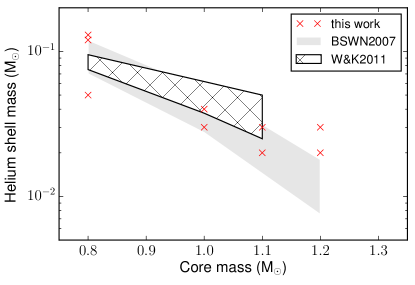
Due to the importance of $T_{\mathrm{core}}$ demonstrated in Woosley & Kasen (2011), we include models with $T_{\mathrm{core}}=10^{7},10^{8}$ K. Finally, we vary $T_{\mathrm{base}}$ from 175 MK to 250 MK. These interface temperatures are intended to be roughly what we would expect a few to several convective turnover times before runaway, based on both our own numerical experiments and the 1D literature. Table 1 lists the details of our model set.

While our models are motivated by the literature they are not necessarily likely to be realized in nature and are not the result of detailed stellar evolution calculations. Our focus is on broadly sampling the parameter space, characterizing the relationships between parameters and possible explosive outcomes, and quantifying the salient trends that emerge. This will guide future work studying particularly interesting parameter configurations using more realistic initial models and detailed nucleosynthesis.

3 Results

3.1 Outcomes

Our broad sampling of parameter space explores several different model configurations. We find a range of outcomes for these models: localized runaway, quasi-equilibrium, and convective runaway. The last column of Table 1 denotes the ultimate outcome of each model.

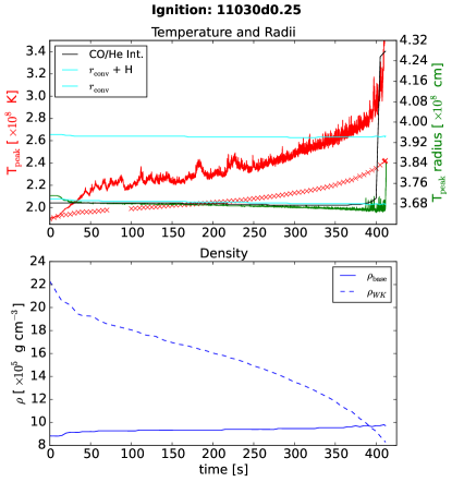
Localized runaways represent possible seeds of deflagration or detonation in the helium shell. All runs in this category have localized volumes of fluid that experience rapid temperature runaway to about 1 GK. They also have peak Mach numbers less than 0.3 before runaway, and less than 0.2 for the majority of the simulated time. Fig. 4 plots some of the key properties of interest over time for an igniting run (model 11030). This plot is representative of the general behavior of runs experiencing localized runaway. The plot demonstrates that the temperature of the hottest cell in the domain initially follows a trend similar to that of the laterally averaged peak temperature. As the model approaches runaway the hottest cell increasingly deviates from the background conditions. We also find that the convectively unstable region moves deeper into the star. This suggests that vigorous burning and the convection it drives can result in significant changes in the density and composition of burning sites (discussed more in §3.4).

Figure 4: Temperature, radius, and density over time for model 11030. Top: Temperature is plotted in red. The solid line is the temperature of the hottest cell in the entire computational domain. The x’s trace the peak laterally averaged temperature. The green, cyan, and black all plot radii. Green is the radius of the hottest cell in the domain. Black is a trace of the core/shell interface based on the radius at which the average $X_{\mathrm{He}}$ composition is 0.9. The cyan plots the base of the convective region and one pressure scale height above this base. The inset is a 2D temperature slice centered on the site of runaway, demonstrating its localized nature. The runaway happens at a boundary, hence half the inset being white (no temperature data outside the boundary). Bottom: The solid line plots the laterally averaged density at the radius of peak average temperature. The dashed line is the critical density above which ignition is expected according to Eq. 1.

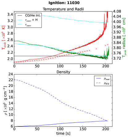
As one might expect, the radius of the hottest cell moves radially inward along with the base of the convectively unstable region. However, at the end we see that this radius moves outward in many models. If convection is able to transport an ignition seed to a significant height above the core/shell interface then it makes “edge-lit” double detonation models workable. In the edge-lit scenario, carbon detonation of the core is triggered by the propagation of the helium detonation wave at the surface of the core. This model is generally disfavored because it has been shown that it requires the initial helium detonation to go off at a substantial height above the core/shell interface (García-Senz et al., 1999; Woosley & Kasen, 2011). If convection is more effective than expected at transporting the detonation seed then the edge-lit scenario needs to be considered more seriously.

Unfortunately, many of the localized runaway events in our models happen near the boundary of the octant being simulated. We stress that we have carried out a full star run for the localized runaway model 08130 (and also in paper I for a 10050 model) and still find localized runaway as well as a radius significantly above the interface. We have also carried out simulations in which the temperature of cells is limited to be below 3.5 MK and see that many localized runaways occur far from the boundary, though the initial runaway happens preferentially at the boundary. So while we are confident the localized runaway is not a boundary effect, the elevated radius of the hottest cell in fig. 4 cannot be ruled out as a boundary effect in all runs. This is an important issue that will be resolved in the next paper in this series, which focuses on the timing, thermodynamics, and geometry of ignition in this suite of simple models.

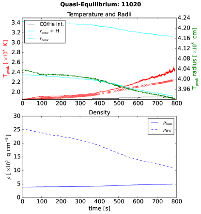
In contrast, quasi-equilibrium simulations balance nuclear burning with convective cooling for many convective turnover times (at least an average of 3.8 or more turnovers, see Table 1 for a range of turnover estimates and §3.4 for how we calculate these). Fig. 5 demonstrates this case for a model we ran for a particularly long time. We cannot say these runs have reached an equilibrium between burning and convective cooling because neither peak nor average base temperatures plateau, nor do we model any energy sinks (cooling). If we had the computational resources to run these simulations indefinitely it may be the case they would experience a runaway. What we demonstrate instead is that these models are stable against immediate runaway, i.e. runaway within a few convective turnover times.

Figure 5: The same plot as in fig. 4 for model 11020, demonstrating quasi-equilibrium.

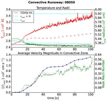
We have also included a model similar to Woosley & Kasen (2011)’s model 8HB, which experiences a helium nova (convective runaway). This model had a higher interface temperature than most runs, 2.5 MK instead of around 1.9 MK, to facilitate reaching runaway conditions without expending more computational resources than necessary. Within the low-Mach limits of Maestro we also find convective runaway, even with the elevated interface temperature. As the base temperature increases from burning, the turnover rate of the convective shell is able to increase without plateauing until the Mach number of the fluid gets too large for us to track. This suggests such a thin shell is able to rapidly transport the energy release of nuclear burning. In contrast to localized runaway, this is a more global phenomenon and could develop into something like a helium nova, as argued in Woosley & Kasen (2011). The time series data for this convective runaway is plotted in Fig. 6. The existence of two regimes, convective and localized runaway, suggests researchers should investigate the transition from one to the other. The conditions of this transition point will be important for determining the minimum helium shell mass capable of achieving localized runaway.

Figure 6: The top plot is the same as in fig. 4 for model 08050. The bottom plot shows the average velocity magnitude in the convective zone as well as the peak Mach number in the domain.

3.2 Temperature

While the mass of the core and helium shell play a primary role in determining the thermodynamic conditions at the base of the shell, there are secondary determinants. Varying evolutionary histories can result in accreting C/O WD primaries of varying temperatures. A history of helium flashes may heat the WD surface. This enables systems with similar mass configurations to have noticeable differences in burning conditions at the core/shell interface.

Our parameterization of the initial model allows us to vary the initial temperature of the actively burning base of the helium shell. However, in our attempts at varying the base temperature we find only a relatively narrow range of options can be feasibly explored with our current methods. Low initial temperatures will either not be able to initiate sufficiently vigorous burning to allow a study of ignition or will establish a trend of growing average base temperature that will steadily build until either ignition or quasi-equilibrium is achieved. However, the computational resources required to reach a dynamically interesting stage of burning with a low initial base temperature can be substantial. Too high a base temperature will either lead to unphysical ignition by not allowing time for convection to be established or will push the convective velocity beyond Maestro’s ability to model. Thus, for a given model we choose an initial base temperature low enough to allow for convection to be established and for several convective turnover times of evolution, and high enough to reach a scientifically interesting stage of burning while using feasible amounts of computational resources.

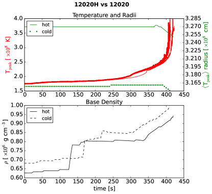
The influence of the isothermal core’s temperature is easier to investigate with our methods. Woosley & Kasen (2011) find that their synthetic spectra and light curves come closest to resembling observations of type Ia’s for their “hot” models in which the accreting C/O WD relaxes into thermodynamic equilibrium with a luminosity of $1~{}\mathrm{L}_{\odot}$ before accretion is modeled. The hotter core enables runaway in thinner shells than the colder core. This motivates our exploration of our own “hot” and “cold” ($10^{8}$ and $10^{7}~{}\mathrm{K}$) models (hot models are indicated with an ’H’ in their label in Tab. 1).

Our results are consistent with that of Woosley & Kasen (2011). Hot cores allow for initiation of localized runaway at lower densities for a given core/shell mass configuration. This is largely due to an expanded core radius in hot runs, and thus a lower density at the core/shell interface where the burning occurs. The lower density favors higher temperatures at runaway as well. In Fig. 7 we compare a hot and cold run to demonstrate these phenomena.

Figure 7: Comparison of several properties for a hot ($10^{8}$ K isothermal core, solid lines) and cold ($10^{7}$ K, dotted and dashed lines) model with a 1.2 $M_{\odot}$ core and 0.02 $M_{\odot}$ shell. Top: In red we plot the global peak temperature. In green we plot the radius of the temperature peak from a lateral average of the 3D data. Bottom: In black we plot the laterally averaged density at the radius plotted in green in the top panel.

3.3 Localized Runaway

We have demonstrated that many of our models achieve localized runaway through bulk diagnostics and time-series data, comparing them to 1D results. This answers a major question we are exploring: is ignition found in 1D codes consistent with 3D models? We argue the localized runaway we find is consistent, though do caution that localized runaway should not be thought of as ignition. The localized runaway reported here may ignite deflagrations or detonations, but there is insufficient evidence and analysis in this paper to make a definitive determination. The next paper in this series will focus in part on determining the likelihood of such ignition. For now, we move to characterizing the localized runaway found in our models.

The 1D studies we have discussed necessarily model ignition as simultaneous across a spherical shell. Fink et al. (2007) contribute 2D simulations including a variety of detonation seed geometries, following up later in Fink et al. (2010) with 2D simulations seeding a single detonation in a larger range of core/shell masses including thin shells. Moll & Woosley (2013) have contributed 2- and 3D studies in which detonation is seeded at multiple points with variations in geometry as well as timing. A key conclusion of these multi-D investigations is that detonation in the helium shell very robustly triggers detonation of the C/O core via radially propagating compression waves generated by the helium detonation’s shock front traversing the shell.

Assumptions about how many detonations to seed, where to seed them, and their timing impact the ultimate outcome of the double detonation. Single-point helium detonations lead to viewing-angle dependences not expected in normal SNe Ia, though the dependence becomes weaker for lighter helium shells (Kromer et al., 2010). If detonated at a great enough altitude above the core/shell interface, helium detonations can directly ignite carbon burning instead of detonating indirectly with converging shock fronts (García-Senz et al., 1999; Woosley & Kasen, 2011; Moll & Woosley, 2013). The size and shape of the detonation can also impact how easily core detonation can be triggered, especially for the thinner shells considered to be the most promising candidates for modeling normal SNe Ia (Moll & Woosley, 2013).

Figure 8: Hotspot properties for model 08130 at $t=130.0$s. Upper left: histogram of the radii of the hotspots, with bin sizes chosen to match the finest level of 3D resolution. Each bin is color-coded to indicate the maximum temperature in the bin. The location where helium’s laterally averaged mass fraction is 0.9 and the base of the convective envelope are indicated. Upper right: histogram of the densities of the hotspots. Again, bins are color-coded based on maximum temperature. The value of Eqn. 1 is indicated. Bottom: projection of the hotspots’ angular location onto a sphere corresponding to the average radius of the hotspots. Hotspot pixel sizes correspond to the finest level’s physical resolution, and where hotspots overlap preference is given to the one with the highest temperature. The extents of the temperature color bar’s bins are set such that each bin contains an equal number of hotspots.

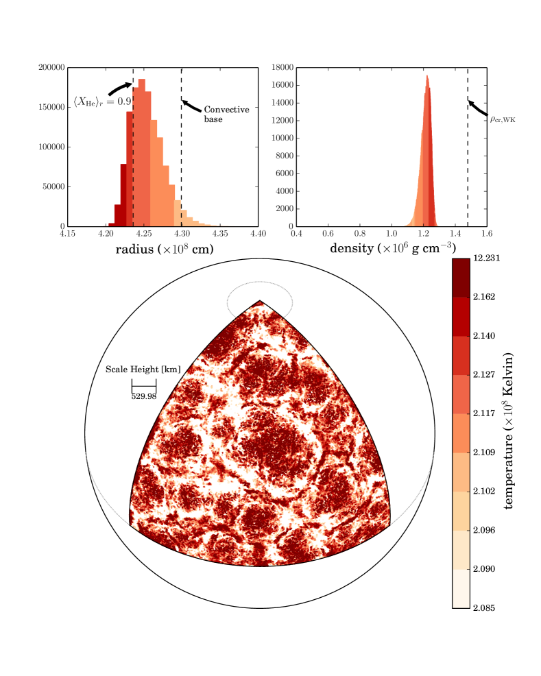
In light of this, what do our models suggest? To assess the conditions that foster ignition we track the hottest 0.005 % of cells in the computational domain immediately prior to runaway. Fig. 8 plots histograms of the radii and densities of these cells in addition to a spherical projection of their angular locations for model 08130 (see Table 1). The spherical projection illustrates the two regions in which volumes of hot fluid develop: at the base of convective inflows and at the intersection of outflows from neighboring convective cells (see §3.4). This is determined by contrasting projections like that in Fig. 8 with renderings of convective outflow like that in Fig. 9. The density histogram includes a reference for a critical runaway density given by Eq. 8 in Woosley & Kasen (2011):

$$\rho_{\mathrm{cr,WK}}=\left(1.68\times 10^{-4}~{}\exp(20/T_{8})\right)^{1/2.3},$$ (1)

where $T_{8}=T/10^{8}$ is the temperature in units of $10^{8}$ K. This is a rough critical density above which violent, hydrodynamic runaway is expected and below which convection is expected to be efficient enough to transport any energy generated by nuclear burning. For the purposes of this paper, we denote it as a critical density above which we expect localized runaway to be possible.

This density is based on 1D models and thus is only fairly compared to lateral averages of quantities in our 3D simulations. Note that Fig. 8 demonstrates localized runaway is achieved even though the hottest cells have densities significantly below this critical density. This is not surprising as the cells trace a 3D model. When we consider laterally averaged quantities, Eq. 1 is often an excellent predictor of ignition. Ignition is achieved almost exactly as the average density at the peak burning region surpasses the (temperature-dependent) critical density in Fig. 4, whereas the same average density is well below the critical value in the quasi-equilibrium case of Fig. 5.

This predictor does not work as well for our models with 0.8 $M_{\odot}$ core masses. These models achieve localized runaway despite being quite a bit below the critical density. This could either be an effect of our models capturing the 3D dynamics and thus of scientific interest, or it could be a result of our models being toward the upper limit of the minimum shell mass the critical density is calculated for in our 0.8 $M_{\odot}$ models. In addition, the critical density is only a rough estimate based on the outcomes of several 1D models. Still, for cores $\geq 1.0~{}M_{\odot}$ it is quite accurate for our models. We will further investigate this critical density and determine a 3D version in the next paper of this series.

Table 2 lays out key properties at the time of runaway for all models that experienced localized runaway. The table includes an estimate of the number of convective turnover times modeled before ignition as well as the lateral averages of temperature and density at the radius of peak burning ($r_{\mathrm{peak}}$). Note that these are values based on the 3D output with a timestamp nearest that of the peak temperature. This is why the peak times tend to end on round numbers—our 3D state is output at most every tenth of a second.

Table 2: Ignition Conditions

model	$t_{\mathrm{peak}}$	$t_{\mathrm{peak}}/\langle\tau_{\mathrm{conv}}\rangle$	$\langle r_{\mathrm{base}}\rangle$	$\langle T_{\mathrm{base}}\rangle$	$\langle\rho_{\mathrm{base}}\rangle$
	[$s$]		[km]	[$\times 10^{8}~{}K$]	[$\times 10^{5}~{}\mathrm{g~{}cm^{-3}}$]
12030H	118.2	8.4	3096.4	2.180	13.877
12030	120.4	6.4	3009.4	2.178	14.541
12020H	420.0	10.3	3261.6	2.480	9.424
12020	410.0	12.4	3163.7	2.410	9.963
11030H	319.5	10.6	3839.8	2.462	7.729
11030	205.0	8.5	3739.1	2.456	7.968
08130H	161.7	3.7	4372.9	2.139	11.464
08130F	137.4	1.2	4251.7	2.096	12.218
08130	130.6	3.3	4259.6	2.069	12.106
08120H	240.0	7.7	4470.0	2.181	10.365
08120	710.0	25.7	4338.7	2.041	11.221

3.4 Convection

The ignition characterized in the previous section is fostered by the complex interplay between nuclear burning and convective dynamics. A detailed understanding of convective evolution is crucial, as illustrated by the conflicting results of Fink et al. (2010) and Woosley & Kasen (2011).

Fink et al. (2010) get their initial 1D models from Bildsten et al. (2007), who assume a fully convective shell all the way up to the point of ignition. Woosley & Kasen (2011) employ a time-dependent convective model based on mixing-length theory, allowing for convection to “freeze out.” If the runaway timescale for a volume of fluid at the base of a convective zone, in the absence of cooling, becomes smaller than the convective turnover timescale, convection is no longer able to cool the helium-burning layer with the same efficiency. It starts to “freeze out.” A fully convective shell requires a larger temperature at its base to achieve runaway than with one in which freeze-out is allowed. The temperature differences translate into entropy differences. In turn, the lower entropy of the cooler base makes possible larger base densities in the Woosley & Kasen (2011) models than those of Fink et al. (2010), even when they are modeling similar core and shell masses. These density discrepancies lead to significant discrepancies in explosive burning and the products yielded.

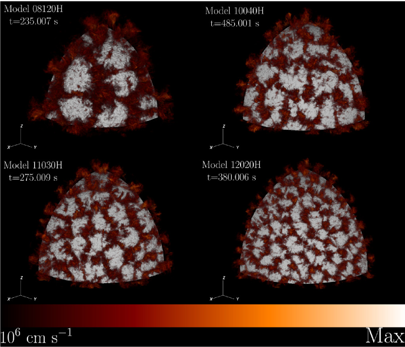
Our analysis of convective dynamics begins by establishing the broad context. Fig. 9 plots volume renderings of radial velocity for several models. These act as a proxy for convective plumes. Higher core masses result in more compact systems with smaller pressure scale heights. Thus we see the typical size of a convective cell grows inversely proportionally to core mass. The hotspots plotted in Fig. 8 occur at the base of convective plumes of cool in-falling fluid and at regions in which outflows of adjacent convective cells collide. The in-falling matter increases the density, setting off more vigorous nuclear burning. A competition between the nuclear burning rate of a volume of fluid and the rate at which it can be transported and cooled by convective flow is established.

Figure 9: Volume rendering of radial velocities for some representative models. Maximum velocities are 2.8, 1.3, 2.0, and 1.7 $\times 10^{7}~{}\mathrm{cm~{}s}^{-1}$ for models 08120H, 10040H, 11030H, and 12020H, respectively.

In our models we see convective dynamics have two key impacts. First, convective overshoot serves to push the region of active burning deeper into the star, thus increasing the ambient density of nuclear burning sites and altering the ambient composition. Second, convection’s ability to respond to increasing nuclear energy generation breaks down for sufficiently energetic burning. This is the freeze-out discussed in Woosley & Kasen (2011).

Convective overshoot is demonstrated in the top plot of Fig. 10 for model 11030. The first process to happen in a model is for convection to be established in response to nuclear burning, the bulk temperature profile, and our initial velocity perturbations (see Fig. 1). This is seen in the plot of the convective timescale at the bottom of Fig. 10. Initially it experiences a steep drop off until stabilizing as convective cells are established. After this we see that the location of the convective base steadily moves radially inward. In response, the radius of peak burning moves deeper into the star resulting in increased ambient density as well as changes in ambient composition. We find in most models that experience localized runaway, peak burning radii tend to stabilize near the location where composition is 90% helium (shell material), 10% carbon (core material). In addition, models in quasi-equilibrium do not have such substantial radial migration of the convective base.

Figure 10: Top: Here we plot: the radius of the cell with the largest nuclear energy generation in the entire domain, $r(\dot{\epsilon}_{\mathrm{peak}})$, in cyan; the radius of this same quantity for the laterally averaged data, also in cyan with “x” markers indicating the timestamp the data was calculated for; the radius at which the lateral average of helium’s mass fraction $\langle X_{\mathrm{He}}\rangle$ is 0.9, in magenta; the radius of the convective base as determined by the radius at which the entropy flattens out (see Fig. 1), in yellow; and the radius at which the lateral average of temperature $\langle T\rangle$ peaks, in black. Bottom: A comparison of a nuclear burning timescale (magenta) with a convective turnover timescale (cyan). See text for details.

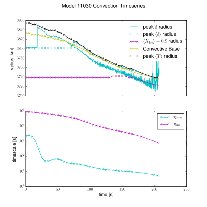
Freeze-out is demonstrated in the bottom of Fig. 10. Here we plot two different timescales. To calculate a minimum nuclear burning timescale we invert the burning rate, $dX_{i}/dt$, for the most rapidly burning species $i$ (for these models, helium). This is done for all radius bins $r$ in our lateral averaging. The minimum value of this radial slice is used as our nuclear timescale $\tau_{\mathrm{nuc}}$. In sum,

$$\tau_{\mathrm{nuc}}=\min_{r}\left(\min_{i}\left\langle\frac{dX_{i}}{dt}\right\rangle^{-1}\right)_{r}.$$ (2)

The other timescale is a conservative estimate of the convective turnover time. Again using laterally averaged data, we invert the velocity magnitude $\langle|\mathbf{U}|\rangle$ and integrate over the convective region,

$$\tau_{\mathrm{conv}}=\int_{r_{b}}^{r_{t}}\left\langle\left|\mathbf{U}(r)\right|\right\rangle^{-1}dr.$$ (3)

$r_{b}$ is the smallest radius at which the radial entropy profile satisfies $ds/dr=0$ and $r_{t}$ is largest radius satisfying this condition. The region is shaded in Fig. 1. This average value is reported in Table 1. In addition, Table 1 includes a calculation of the minimum and maximum estimates for turnover times by simply dividing the lengthscale $r_{t}-r_{b}$ by the maximum and minimum velocities in the convecting region, respectively. We want to stress these are conservative estimates. Not all plumes that form will extend the full lengthscale, and there may be plumes with faster fluid than in other plumes.

In the timescale plot of Fig. 10 we see that as model 11030 approaches runaway the nuclear burning timescale drops more rapidly than the convective turnover timescale. We note that the focus is not on the magnitudes of the timescales but their changes. The highly nonlinear nature of nuclear burning make comparisons of the rate’s magnitude at any given time with other timescales uninformative. The changes however suggest the nuclear burning rate is shrinking faster than the convective turnover rate as runaway is approached, suggesting a degree of freeze-out.

In contrast, quasi-equilibrium models and the convective runaway model have relatively flat peak burning radii. Their convection is able to respond to nuclear burning before any localized runaway can develop.

3.5 Varying $\delta$ and Comparison with a 1D Model

Figure 11: Zoomed-in X-Y slices of temperature at the base of the convecting helium envelope for models 11030 and 11030d0.25 at initial and late times (see subplot labels). Cell edges are overlayed. The two white vertical lines mark, left-to-right, the radius at which the lateral average of the velocity magnitude is 25% and 50% of its peak.

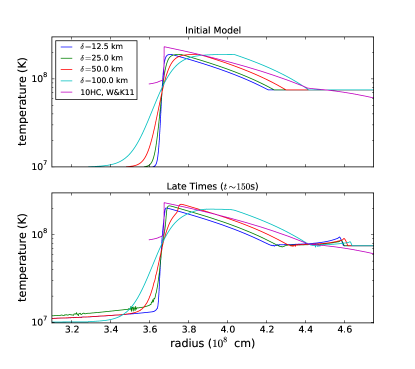
As discussed in §2.2, we have carried out an additional numerical experiment exploring the impact of varying the $\delta$ parameter that determines the sharpness of the transition from core to shell (see Paper I for details). In Fig. 12 we plot the temperature profiles of models 11030d0.25, 11030d0.5, 11030, and 11030d2, which have identical initial models except for their $\delta$ parameters: 12.5, 25, 50, and 100 km, respectively. In addition, we plot the temperature profile of model 10HC from Woosley & Kasen (2011) at a time near ignition (model data courtesy of Woosley, private communication). The radius of 10HC is offset by 500 km to facilitate comparison of transition widths. We plot both the initial temperature profile and those from later times. Initially, our default $\delta$ value results in a more gradual transition than in 10HC. At later times, the temperature profile develops a more pronounced peak like that of 10HC, though the transition continues to be less sharp than 10HC and leaves a substantial amount of hot fluid below the temperature peak. We see that our smaller $\delta$ values, in particular that of 11030d0.25, are about as sharp as that of 10HC.

Figure 12: Comparison of temperature profiles for varying $\delta$. Top: The temperature profiles of initial models with varying $\delta$ along with a realistic 1D reference (model 10HC from Woosley & Kasen (2011), radius shifted $-500$ km to facilitate comparison). Bottom: The same reference model along with profiles for the laterally averaged temperature data from models 11030d0.25, 11030d0.5, 11030, 11030d2 after $\sim 150$s of evolution.

One potential worry with the thicker transition is that it allows a thin shell of hot fluid (80-90% of the peak interface temperature) to exist below the region initially unstable to convection (see Fig.1). If convection is not well-established in these hot shells as the model approaches runaway then it becomes hard to determine if the runaway is a result of the uncooled hot shell in some initial models or the convective dynamics. To address this concern, we plot slices of temperature at $t=0$ and late times for 11030d0.25 and 11030 in Fig. 11. This plot includes white vertical lines marking the radius at which the laterally averaged velocity magnitude is 25% and 50% of its peak value. This gives the reader an idea of how much convective cooling penetrates. The late-time temperature profile develops into a thin, hot layer for both $\delta$ values, with similar velocity penetration. This demonstrates that even with a thicker transition the cooling in our models penetrates to the thin shell of vigorous burning. The primary impact of the smaller $\delta$ is to shift the radius at which the thin, hot layer develops. This is an expected imprint of the initial model, as the thinner $\delta$ locates a more concentrated shell of hot fluid at a lower radius, as seen in Fig. 11. In addition, the thicker $\delta$ results in a larger region of intermediate temperature below the thin, hot layer. Finally, we note that a history of helium flashes can heat the base of the convecting envelope. Nature may in fact realize configurations in which hot fluid exists below the convectively unstable region.

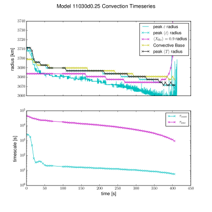
We find that all of the runs with varied $\delta$’s also experience localized runaway. In addition, the convective dynamics reported in previous sections are qualitatively insensitive to varied $\delta$. Figs. 13 and 14 illustrate this using model 11030d0.25. We also see a new result: the dramatic rise of the typical radius at which helium’s mass fraction satisfies $X_{\mathrm{He}}=0.9$. This suggests substantial mixing as carbon is dredged up, displacing helium. This will be explored in more detail in the next paper in this series.

Figure 13: Same as Fig. 4 for model 11030d0.25

Figure 14: Same as Fig.6 for model 11030d0.25

4 Conclusions and Discussion

We have explored 18 physically motivated, simple models of convective burning in sub-Chandrasekhar carbon/oxygen white dwarfs with an accreted, low-mass helium shell, as well as 3 supplemental models exploring a new numerical experiment of the impact of an initial model parameter. These systems have been modeled in 3D with detailed microphysics using the low-Mach hydrodynamics code Maestro. These are the first 3D simulations of this phase of evolution for such a broad suite of models, and we have drastically expanded the diagnostics and analysis in comparison to Paper I.

As we make clear in §2, our models are simple and limited in the number of species and reactions we track. This is sufficient for our focus on exploring a large number of model systems and capturing the dominant energetics and general dynamical trends. Our findings here will serve as the foundation for future work focused on a smaller number of more detailed models. From this set of simple models we can draw several important insights into potential double detonation SNe Ia or .Ia progenitors as well as other runaway events involving sub-Chandrasekhar white dwarfs with envelopes of accreted helium, such as possible helium novae.

We find that localized runaway is indeed achievable in 3D. Whether this develops into a deflagration or detonation will be the focus of future work. In particular, it would be valuable to make use of the Maestro-to-Castro mapping developed in Malone et al. (2014). Like Woosley & Kasen (2011), we find that hotter cores allow for localized runaway to develop at lower densities than in models with cooler cores. Thus, hotter cores are able to achieve runaway with thinner (lower mass) helium shells than cooler cores of the same mass.

Our results indicate that the complex dynamics of 3D convection should not be neglected in investigations of double detonation progenitor models. In cases of localized runaway, we find evidence of convective overshoot and a steady freeze-out of convection. These effects substantially impact the density, temperature, and composition of the region in which localized runaway is initiated.

Future papers in this series will characterize the geometry, thermodynamics, statistics, and timing of ignition in greater detail, carry out more realistic simulations making use of 1D stellar evolution for initial models and larger reaction networks, and map our low-Mach results into the compressible code Castro to track the development of deflagration or detonation.

Appendix A An Improved Low Mach Number Equation Set

In this Appendix, we discuss the improved low Mach number equation set used for the simulations presented in this paper, and highlight the differences from the algorithm presented in Nonaka et al. (2010). We also discuss the effects of this improved model on some standard test problems.

Recently, both Klein & Pauluis (2012) and Vasil et al. (2013) introduced a new term in the vertical momentum equation for low Mach number stratified flows that enforces conservation of total energy in the low Mach number system in the absence of external heating or viscous terms. To compare the new system with the origianl Maestro equations, we first define $\rho^{\ast},{\bf{U}}^{\ast},p^{\ast},$ and $T^{\ast},$ as the density, velocity, pressure, and temperature, respectively, in the low Mach number system, in keeping with the notation used in Durran (1989) and Klein & Pauluis (2012). The perturbational quantities, $\rho^{\prime,\ast}=\rho^{\ast}-\rho_{0}$ and $p^{\prime,\ast}=p^{\ast}-p_{0},$ are analogous to those in the compressible system. The quantities defining the starred fluid approximate, but are not identical to, the quantities defining the fully compressible fluid.

The following equations were derived in Almgren et al. (2006a) for low Mach number stratified flow with a general equation of state:

$$\frac{\partial\rho^{\ast}}{\partial t}+\nabla\cdot(\rho^{\ast}{\bf{U}}^{\ast}) = 0\enskip,$$

$$\frac{\partial{\bf{U}}^{\ast}}{\partial t}+{\bf{U}}^{\ast}\cdot\nabla{\bf{U}}^{\ast}+\frac{1}{\rho^{\ast}}{\nabla}p^{\prime,\ast} = -\frac{\rho^{\prime,\ast}}{\rho^{\ast}}g\mathbf{e}_{r}\enskip,$$ (A1)

with the constraint of the form,

$$\nabla\cdot(\beta_{0}(r){\bf{U}}^{\ast})=\beta_{0}\sigma\mathcal{H}\enskip,$$ (A2)

where

$$\beta_{0}(r)=\beta(0)\exp\left({\int_{0}^{r}\frac{dp_{0}/dr^{\prime}}{\Gamma_{1_{0}}p_{0}(r^{\prime})}\,dr^{\prime}}\right)\enskip$$

and $\sigma=p_{T}/(\rho c_{p}p_{\rho})$ (Almgren et al., 2006b), which in the case of an ideal gas reduces to $1/(c_{p}T).$ Also, we define $\Gamma_{1_{0}}$ as the lateral average of the first adiabatic exponent,

$$\Gamma_{1}\equiv\left.{d(\log p)}/{d(\log\rho)}\right|_{s}\enskip.$$ (A3)

Klein & Pauluis (2012) modify the vertical momentum equation by noting that a low Mach number representation of total energy is conserved if, in moving from the compressible to the low Mach number system, one substitutes $1/\rho\rightarrow 1/\rho^{\ast}-(1/\rho^{\ast})^{2}(\partial\rho^{\ast}/\partial p_{0})|_{s}(p^{\ast}-p_{0})$ instead of $1/\rho\rightarrow 1/\rho^{\ast}$ in the momentum equation, resulting in

$$\frac{\partial{\bf{U}}^{\ast}}{\partial t}+{\bf{U}}^{\ast}\cdot\nabla{\bf{U}}^{\ast}+\frac{1}{\rho^{\ast}}{\nabla}p^{\prime,\ast}=\dfrac{1}{\rho^{\ast}}\left(\left.\dfrac{\partial\rho^{\ast}}{\partial p_{0}}\right|_{s}p^{\prime,\ast}-\rho^{\prime,\ast}\right)g\mathbf{e}_{r}\;.$$ (A4)

Vasil et al. (2013) instead construct the additional term by deriving the low Mach number momentum equation from Lagrangian analysis, starting from conservation of total energy. The momentum equation given in Vasil et al. (2013) uses the assumption from Almgren et al. (2006a) that $\Gamma_{1}$ can be approximated by $\Gamma_{1_{0}}$, and can be written in the form

$$\frac{\partial{\bf{U}}^{\ast}}{\partial t}+{\bf{U}}^{\ast}\cdot\nabla{\bf{U}}^{\ast}+\frac{\beta_{0}}{\rho^{\ast}}{\nabla}\left(\frac{p^{\prime,\ast}}{\beta_{0}}\right)=-\dfrac{\rho^{\prime,\ast}}{\rho^{\ast}}g\mathbf{e}_{r}$$ (A5)

We note that (A5) is analytically equivalent to (A4) when $\Gamma_{1}\equiv\Gamma_{1_{0}}$.

An essential component of the solution procedure for low Mach number equation sets is solving a variable coefficient Poisson equation for the perturbational pressure. The Poisson equation can be derived by substituting the constraint into the divergence of the momentum equation,

$$\nabla\cdot\left(\frac{\beta_{0}}{\rho^{\ast}}\nabla p^{\prime,\ast}\right) = \nabla\cdot(\beta_{0}A^{\ast})-\beta_{0}\frac{\partial(\sigma{\mathcal{H}})}{\partial t},$$ (A6)

with

$$A^{\ast}=-[{\bf{U}}^{\ast}\cdot\nabla{\bf{U}}^{\ast}]-\frac{(\rho^{\ast}-\rho_{0})}{\rho^{\ast}}{\bf g}$$

Using their formulation, Vasil et al. (2013) show that one can instead solve

$$\nabla\cdot\left[\frac{\beta_{0}^{2}}{\rho^{\ast}}\nabla\left(\frac{p^{\prime,\ast}}{\beta_{0}}\right)\right] = \nabla\cdot(\beta_{0}A^{\ast})-\beta_{0}\frac{\partial(\sigma{\mathcal{H}})}{\partial t}$$ (A7)

for $p^{\prime,\ast}.$ Analytically, this looks very similar to the original equations, and numerically, it allows one to reuse the original solver, simply modifying the coefficients ($\beta_{0}^{2}/\rho^{\ast}$ as opposed to $\beta_{0}/\rho^{\ast}$) and the interpretation of the variable being solved for ($p^{\prime,\ast}/\beta_{0}$ as opposed to $p^{\prime,\ast}$). While exactly the same solver can be used to solve Equation (A7) as to solve Equation (A6), we note that solving for $p^{\prime,\ast}$ in the new constraint may take more computational effort. This arises because in Equation (A6) the coefficients of $p^{\prime,\ast}$ are close to one, since $\beta_{0}$ is a density-like variable that is close to $\rho_{0}$ (and in fact identically equals $\rho_{0}$ for an isentropically stratified atmosphere). The coefficients in Equation (A7) are, by contrast, similar to $\beta_{0}(r),$ which can have large variation over the scale heights within a single calculation.

We note also that the simplification allowed by writing the equation for $p^{\prime,\ast}$ in the form Equation (A7) as opposed to more elaborate formulations used in Klein & Pauluis (2012) occur under the assumptions that the flow is non-adiabatic and the base state is constant in time. The implications of adiabaticity and a time-varying base state are subjects of future work.

A.1 Test Problems

Here we look at the impact of the different formulations of the momentum equation on two test problems we have used in the development of Maestro as well as one of our science cases. In Vasil et al. (2013) a study of linear gravity waves using the two different formulations as implemented in the Maestro code demonstrated that the eigenfunctions, energy conservation properties and pseudo-energy conservation were as expected. We refer the reader interested in those results to Vasil et al. (2013).

A.1.1 Reacting Bubble Rise

In Almgren et al. (2008) we showed an example of three burning bubbles in a stratified white dwarf atmosphere (modeled in a plane-parallel geometry, for convenience). The bubbles are buoyant and rise and roll up as nuclear reactions release heat in the hotter locations. Here we revisit that problem with the modified momentum equation. Figure 15 shows a comparison of the temperature field ($T^{\ast}={\widehat{T}}(p_{0},e^{\ast})$). for the simulation using the new formulation vs. the original equations. As we can see, the new formulation generates slightly wider bubbles.

Figure 15: Comparison of burning bubbles with the new formulation and the original formulation of the Maestro equation set.

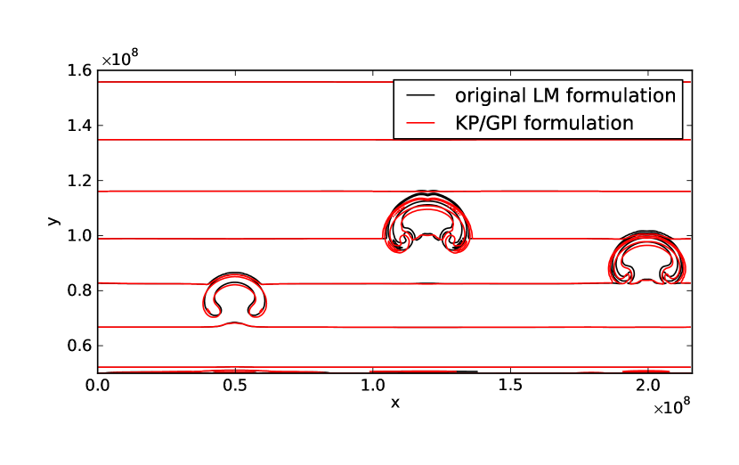
This difference in width is consistent with an observation made in Almgren et al. (2006a), where we compared low Mach number simulations of non-reacting buoyant bubbles with compressible simulations. There we saw variation between the bubbles as calculated with the different methods (including between the two compressible formulations), but observed that the bubbles that evolved via the low Mach number equation set were consistently narrower than the fully compressible bubbles. The fact that the new formulation generates slightly wider bubbles suggests in a general sense that the solution with the new formulation is closer to the fully compressible solution than that generated with the original formulation.

This test problem is distributed with the public version of Maestro as reacting_bubble.

A.1.2 Internally Driven Convection

A simple test of convection driven by an analytic heating source was shown in Almgren et al. (2008) and again in Nonaka et al. (2010). The details of the setup and heating term are given in Section 4.3 of Almgren et al. (2008). The basic idea of this problem is that there is a convectively unstable region bounded above and below by stable regions. An analytic heat source at the base of the unstable layer drives convection. The top of the convective region essentially spans to the top of the atmosphere, up to the point where the density drops off steeply. We considered the convectively unstable layer to be the “region of interest” for comparison with results from a compressible code, and we found good agreement between the original Maestro equations and the fully compressible solution. Here we compare results from simulations using the new formulation against both the original results and the compressible results. The compressible comparison for this paper is done with the CASTRO code (Almgren et al., 2010).

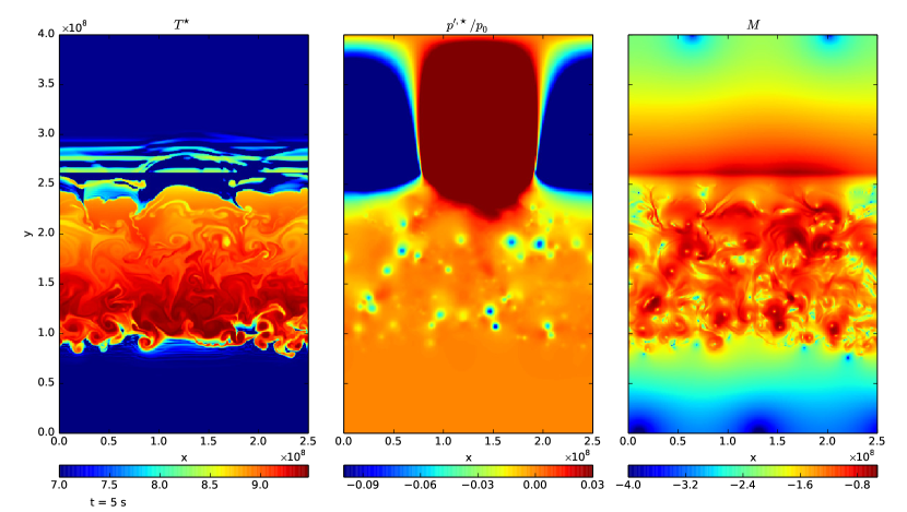
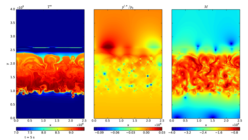
For the calculations presented here, as in the previous two works, a plane-parallel approximation is used for the stellar atmosphere, and $320\times 512$ cells are used to cover the the domain spanning $2.5\times 10^{8}~{}\mathrm{cm}$ in the horizontal direction and $4.0\times 10^{8}~{}\mathrm{cm}$ in the vertical. In Figure 16 we show plots of $T^{\ast},$ $p^{\prime,\ast}/p_{0}$, and Mach number for the the original and new algorithms. Two things are immediately apparent. First, in the convective region, roughly between $10^{8}$ cm and $2.5\times 10^{8}$ cm, we see good agreement between the original algorithm and the new version. The temperature field and Mach number in that region agree nicely. However we also note that above the convective region, the solutions differ. This is precisely the location of the surface of the star, so the density drops sharply to the cutoff value here. We notice that in the new model, the Mach number is much lower in this surface region and $p^{\prime}/p_{0}$ is also much lower (for the latter, we note that the plots use different scales to bring out the details in each case). While these differences do not appear to influence the behavior of the convective region, the large $M$ in this surface region does have implications for the timestep. Overall, the new model seems better behaved in the surface layer. Looking at the stable region beneath the convective layer, we do not see much of a difference between the two models.

Figure 16: $T^{\ast}$, $p^{\prime,\ast}/p_{0}$, and Mach number for the convection test problem using the original (top) and new (bottom) algorithms. Note due to the large difference in $p^{\prime,\ast}/p_{0}$ between the two runs, the original formulation is clipped at the upper value of the plot range. In reality, $p^{\prime,\ast}/p_{0}$ is two orders-of-magnitude larger in the original formulation than in the new energy formulation in the region above the atmosphere.

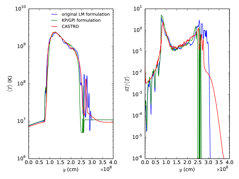
As we did when we previously looked at this test problem, we present two diagnostics: the lateral average of the temperature, $T^{\ast},$

$$\left\langle T\right\rangle_{j}=\frac{1}{N_{x}}\sum_{i=1}^{N_{x}}T_{i,j}\enskip,$$ (A8)

and the RMS fluctuations:

$$(\delta T)_{j}=\left[\frac{1}{N_{x}}\sum_{i=1}^{N_{x}}(T_{i,j}-\langle T\rangle_{j})^{2}\right]^{1/2}\enskip,$$ (A9)

where $N_{x}$ is the number of cells in the lateral direction. Figure 17 shows the profiles of $\langle T\rangle$ and $\delta T/\langle T\rangle$ as a function of height. In the region of interest, the convective layer, we see that all the solutions agree strongly. The differences outside of the convective layer also seem minimal. The increase in $T$ that is seen above the convective layer for the compressible solution is because in the compressible code, the material above the atmosphere is not in hydrostatic equilibrium (it has reached our cutoff density) and rains down onto the surface. This does not have a large dynamic effect because there is not much mass there.

Figure 17: $\langle T\rangle$ and $\delta T/\langle T\rangle$ as a function of height for the convection problem, comparing the original Maestro implementation, the new energy formulation, and the compressible solution from CASTRO.

This test problem is distributed with the public version of Maestro as test_convect.

Appendix B Nuclear Reaction Energetics

To demonstrate that we utilize the smallest set of reactions and isotopes capable of yielding the dominant energetics we calculate the rates for relevant reactions using MESA’s flexible and extensive reaction network module (Paxton et al., 2011, 2013). MESA uses multiple sources for reaction rates, including Sakharuk (2006); Angulo et al. (1999); Caughlan & Fowler (1988). As we do in our own Maestro network, we scale the ¹²C($\alpha,\gamma$)¹⁶O (CagO) reaction by 1.7 (Weaver & Woosley, 1993; Garnett, 1997). The code, data, and configuration for these MESA calculations are distributed in the Maestro repository.

To explore how the reactions highlighted by others (see §2.1) might contribute to the energetics leading into thermonuclear runaway, our MESA calculations use a composition that allows all the relevant reactions to occur and is a reasonable reflection of what we expect in nature. We assume a core of 49.5% ${}^{12}\rm{C}$ and ${}^{16}\rm{O}$, 1% ${}^{22}\rm{Ne}$, and a shell of 99% ${}^{4}\rm{He}$, 1% ${}^{14}\rm{N}$. Since the energy release of ${}^{14}\rm{N}(e^{-},\nu)^{14}\rm{C}(\alpha,\gamma)^{18}\rm{O}$ (NCO) is dominated by the alpha capture on the intermediate ${}^{14}\rm{C}$, 10% of the ${}^{14}\rm{N}$ is converted into ${}^{14}\rm{C}$. The site of active burning is assumed to be 10% core material, 90% shell material as it is in the simulations being reported here. Finally, all mass fractions are reduced by about 5% to allow for 5% of ${}^{1}\rm{H}$ so that the ¹²C(p, $\gamma$)¹³N($\alpha$,p)¹⁶O (CagO-bypass) reaction can proceed. The resulting mass fractions are $\mathrm{X}_{{}^{1}\mathrm{H}}=0.05$, $\mathrm{X}_{{}^{4}\mathrm{He}}=0.84645$, $\mathrm{X}_{{}^{12}\mathrm{C}}=0.047$, $\mathrm{X}_{{}^{14}\mathrm{N}}=0.0077$, $\mathrm{X}_{{}^{14}\mathrm{C}}=0.00085$, $\mathrm{X}_{{}^{16}\mathrm{O}}=0.047$, $\mathrm{X}_{{}^{22}\mathrm{Ne}}=0.001$. In the pre-explosive dynamics leading up to thermonuclear runaway the sites of nuclear burning have $T\approx 200$ MK, $\rho\approx 10^{5}$–$10^{6}~{}\mathrm{g~{}cm^{-3}}$ (see §2.2). The most energetic reaction rates for these conditions and the given composition are plotted in Fig 18.

Figure 18: Energy generation of dominant reactions

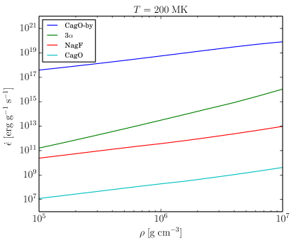
The forward NCO reaction does not become faster than the back-reaction until about $\rho\approx 4\times 10^{6}~{}\mathrm{g~{}cm^{-3}}$ and even then is only marginally faster for the densities considered here, so it is not included in the figure. A much more important consequence of a shell with ${}^{14}\mathrm{N}$ is the quite energetic NagF reaction which can generate an appreciable fraction of the amount of energy generated by the triple-alpha reaction. The triple-alpha reaction still dominates and the dynamics we demonstrate here will be similar with or without the NagF reaction, except that ignition may be achieved more quickly with it. For simplicity, we neglect it in this study. A future study building on this work will explore more detailed nucleosynthesis and the impact of using a larger reaction network.

The CagO-bypass reaction is incredibly energetic. We can only justify neglecting this reaction in our calculations because we are considering pure helium accretion with no free protons before thermonuclear runaway conditions of $T\approx 1$ GK are achieved. As discussed in Shen & Bildsten (2009), even in the event of no protons in the envelope, once conditions of $T\approx 1$ GK are met alpha-chain reactions of ${}^{24}\mathrm{Mg}$ and higher can yield intermediate protons, and the ${}^{14}\rm{N}(\alpha,\gamma)^{18}\rm{F}(\alpha,p)^{21}\rm{Ne}$ reaction directly yields protons (in the pre-explosive regime the ${}^{18}\rm{F}$ is unable to alpha-capture at an appreciable rate). Thus the CagO-bypass reaction must be included for any studies of the sub-M_Ch ignition regime.

From these rate calculations we conclude the triple-alpha reaction dominates energy generation in the pre-ignition conditions and expected composition of C/O WD helium-accretors.

References

- Alastuey & Jancovici (1978) Alastuey, A., & Jancovici, B. 1978, ApJ, 226, 1034
- Almgren et al. (2008) Almgren, A. S., Bell, J. B., Nonaka, A., & Zingale, M. 2008, ApJ, 684, 449
- Almgren et al. (2006a) Almgren, A. S., Bell, J. B., Rendleman, C. A., & Zingale, M. 2006a, ApJ, 637, 922
- Almgren et al. (2006b) —. 2006b, ApJ, 649, 927
- Almgren et al. (2010) Almgren, A. S., Beckner, V. E., Bell, J. B., et al. 2010, ApJ, 715, 1221
- Angulo et al. (1999) Angulo, C., Arnould, M., Rayet, M., et al. 1999, Nuclear Physics A, 656, 3
- Bildsten et al. (2007) Bildsten, L., Shen, K. J., Weinberg, N. N., & Nelemans, G. 2007, ApJ, 662, L95
- Branch et al. (1993) Branch, D., Fisher, A., & Nugent, P. 1993, AJ, 106, 2383
- Brooks et al. (2015) Brooks, J., Bildsten, L., Marchant, P., & Paxton, B. 2015, The Astrophysical Journal, 807, 74
- Brown et al. (2011) Brown, W. R., Kilic, M., Allende Prieto, C., & Kenyon, S. J. 2011, MNRAS, 411, L31
- Caughlan & Fowler (1988) Caughlan, G. R., & Fowler, W. A. 1988, Atomic Data and Nuclear Data Tables, 40, 283
- Drout et al. (2013) Drout, M. R., Soderberg, A. M., Mazzali, P. A., et al. 2013, ApJ, 774, 58
- Durran (1989) Durran, D. R. 1989, 46, 1453
- Fink et al. (2007) Fink, M., Hillebrandt, W., & Röpke, F. K. 2007, A&A, 476, 1133
- Fink et al. (2010) Fink, M., Röpke, F. K., Hillebrandt, W., et al. 2010, A&A, 514, A53
- García-Senz et al. (1999) García-Senz, D., Bravo, E., & Woosley, S. E. 1999, A&A, 349, 177
- Garnett (1997) Garnett, D. R. 1997, Nuclear Physics A, 621, 27
- Geier et al. (2013) Geier, S., Marsh, T. R., Wang, B., et al. 2013, Astronomy & Astrophysics, 554, A54
- Graboske et al. (1973) Graboske, H. C., Dewitt, H. E., Grossman, A. S., & Cooper, M. S. 1973, ApJ, 181, 457
- Hillebrandt et al. (2013) Hillebrandt, W., Kromer, M., Röpke, F., & Ruiter, A. 2013, Frontiers of Physics, 8, 116
- Hunter (2007) Hunter, J. D. 2007, Computing In Science & Engineering, 9, 90
- Itoh et al. (1979) Itoh, F., Honda, T., & Suzuki, K. 1979, Journal of the Physical Society of Japan, 46, 1201
- Ivezic et al. (2008) Ivezic, Z., Tyson, J. A., Abel, B., et al. 2008, ArXiv e-prints, arXiv:0805.2366
- Klein & Pauluis (2012) Klein, R., & Pauluis, O. 2012
- Kromer et al. (2010) Kromer, M., Sim, S. A., Fink, M., et al. 2010, ApJ, 719, 1067
- Li et al. (2011) Li, W., Leaman, J., Chornock, R., et al. 2011, MNRAS, 412, 1441
- Liu et al. (2015a) Liu, Z.-W., Moriya, T. J., Stancliffe, R. J., & Wang, B. 2015a, Astronomy & Astrophysics, 574, A12
- Liu et al. (2015b) Liu, Z.-W., Stancliffe, R. J., Abate, C., & Wang, B. 2015b, The Astrophysical Journal, 808, 138
- Livne (1990) Livne, E. 1990, ApJ, 354, L53
- Livne & Arnett (1995) Livne, E., & Arnett, D. 1995, ApJ, 452, 62
- Livne & Glasner (1990) Livne, E., & Glasner, A. S. 1990, ApJ, 361, 244
- Livne & Glasner (1991) —. 1991, ApJ, 370, 272
- Malone et al. (2014) Malone, C. M., Nonaka, A., Woosley, S. E., et al. 2014, ApJ, 782, 11
- Moll & Woosley (2013) Moll, R., & Woosley, S. E. 2013, The Astrophysical Journal, 774, 137
- Nelemans (2005) Nelemans, . 2005, The Astrophysics of Cataclysmic Variables and Related Objects, 330
- Nomoto (1982a) Nomoto, K. 1982a, ApJ, 257, 780
- Nomoto (1982b) —. 1982b, ApJ, 253, 798
- Nonaka et al. (2010) Nonaka, A., Almgren, A. S., Bell, J. B., et al. 2010, ApJS, 188, 358
- Nonaka et al. (2012) Nonaka, A., Aspden, A. J., Zingale, M., et al. 2012, The Astrophysical Journal, 745, 73
- Paxton et al. (2011) Paxton, B., Bildsten, L., Dotter, A., et al. 2011, ApJS, 192, 3
- Paxton et al. (2013) Paxton, B., Cantiello, M., Arras, P., et al. 2013, ApJS, 208, 4
- Pérez & Granger (2007) Pérez, F., & Granger, B. E. 2007, Computing in Science and Engineering, 9, 21
- Phillips (1993) Phillips, M. M. 1993, ApJ, 413, L105
- Piro (2015) Piro, A. L. 2015, ApJ, 801, 137
- Ruiter et al. (2011) Ruiter, A. J., Belczynski, K., Sim, S. A., et al. 2011, MNRAS, 417, 408
- Sakharuk (2006) Sakharuk, A. 2006, in AIP Conference Proceedings, Vol. 819 (AIP), 118–122
- Shen & Bildsten (2009) Shen, K. J., & Bildsten, L. 2009, The Astrophysical Journal, 699, 1365
- Shen & Bildsten (2014) Shen, K. J., & Bildsten, L. 2014, ApJ, 785, 61
- Shen & Moore (2014) Shen, K. J., & Moore, K. 2014, The Astrophysical Journal, 797, 46
- Sim et al. (2010) Sim, S. A., Röpke, F. K., Hillebrandt, W., et al. 2010, ApJ, 714, L52
- Timmes (2008) Timmes, F. X. 2008, Stellar Equations Of State, ,
- Timmes & Swesty (2000) Timmes, F. X., & Swesty, F. D. 2000, ApJS, 126, 501
- Townsley et al. (2012) Townsley, D. M., Moore, K., & Bildsten, L. 2012, The Astrophysical Journal, 755, 4
- Turk et al. (2011) Turk, M. J., Smith, B. D., Oishi, J. S., et al. 2011, ApJS, 192, 9
- Vasil et al. (2013) Vasil, G. M., Lecoanet, D., Brown, B. P., Wood, T. S., & Zweibel, E. G. 2013, ApJ, 773, 169
- Wang et al. (2013) Wang, B., Justham, S., & Han, Z. 2013, A&A, 559, A94
- Warner (1995) Warner, B. 1995, Astrophysics and Space Science, 225, 249
- Weaver & Woosley (1993) Weaver, T. A., & Woosley, S. E. 1993, Phys. Rep., 227, 65
- Weaver et al. (1978) Weaver, T. A., Zimmerman, G. B., & Woosley, S. E. 1978, ApJ, 225, 1021
- Woosley & Kasen (2011) Woosley, S. E., & Kasen, D. 2011, ApJ, 734, 38
- Woosley et al. (1986) Woosley, S. E., Taam, R. E., & Weaver, T. A. 1986, ApJ, 301, 601
- Woosley & Weaver (1994) Woosley, S. E., & Weaver, T. A. 1994, ApJ, 423, 371
- Zingale et al. (2009) Zingale, M., Almgren, A. S., Bell, J. B., Nonaka, A., & Woosley, S. E. 2009, ApJ, 704, 196
- Zingale et al. (2013) Zingale, M., Nonaka, A., Almgren, A. S., et al. 2013, ApJ, 764, 97
- Zingale et al. (2011) Zingale, M., Nonaka, A., Almgren, A. S., et al. 2011, The Astrophysical Journal, 740, 8