Optimal Learning Rates for Localized SVMs
Abstract
One of the limiting factors of using support vector machines (SVMs) in large scale applications are their super-linear computational requirements in terms of the number of training samples. To address this issue, several approaches that train SVMs on many small chunks of large data sets separately have been proposed in the literature. So far, however, almost all these approaches have only been empirically investigated. In addition, their motivation was always based on computational requirements. In this work, we consider a localized SVM approach based upon a partition of the input space. For this local SVM, we derive a general oracle inequality. Then we apply this oracle inequality to least squares regression using Gaussian kernels and deduce local learning rates that are essentially minimax optimal under some standard smoothness assumptions on the regression function. This gives the first motivation for using local SVMs that is not based on computational requirements but on theoretical predictions on the generalization performance. We further introduce a data-dependent parameter selection method for our local SVM approach and show that this method achieves the same learning rates as before. Finally, we present some larger scale experiments for our localized SVM showing that it achieves essentially the same test performance as a global SVM for a fraction of the computational requirements. In addition, it turns out that the computational requirements for the local SVMs are similar to those of a vanilla random chunk approach, while the achieved test errors are significantly better.
Keywords: least squares regression, support vector machines, localization
1 Introduction
Based on a training set of i.i.d. input/output observations drawn from an unknown distribution on , where and , the goal of non-parametric regression is to find a function such that important characteristics of the conditional distribution , , can be recovered. For instance, an approximating the conditional mean , , is sought in the non-parametric least squares regression. This classical non-parametric regression problem has been extensively studied in the literature, where a general reference is the book (Györfi et al., 2002), presenting plenty of results concerning the non-parametric least squares regression.
In the literature, there are many learning methods that solve the non-parametric regression problems, some of them are e.g. described in (Györfi et al., 2002; Koenker, 2005; Simonoff, 1996). In this paper, we utilize some kernel-based regularized empirical risk minimizers, also known as support vector machines (SVMs), which solve the regularized problem
| (1) |
Here, is a fixed real number and is a reproducing kernel Hilbert space (RKHS) over with reproducing kernel , see e.g. (Aronszajn, 1950; Berlinet and Thomas-Agnan, 2004; Steinwart and Christmann, 2008a). Besides, denotes the empirical risk of a function , that is
where is the empirical measure associated to the data defined by with Dirac measure at . Note that the empirical SVM solution exists and is unique (cf. Steinwart and Christmann, 2008a, Theorem 5.5) whenever the loss is convex in its last argument. Moreover, an SVM is -risk consistent under a few assumptions on the RKHS and the regularization parameter , see (Steinwart and Christmann, 2008a, Section 6.4) for more details. Besides, it is worth mentioning that the ability to choose the RKHS as well as the loss function in (1) provides the possibility to flexibly apply SVMs to various learning problems. Namely, the learning target is modeled by the loss function, e.g. the least squares loss is used to estimate the conditional mean. Moreover, since RKHSs are defined on arbitrary , data types that are not -valued can be handled, too. Furthermore, SVMs are enjoying great popularity, since they can be implemented and applied in a relatively simple way and only have a few free parameters that can usually be determined by cross validation.
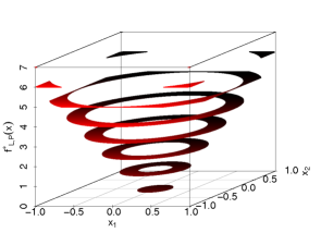
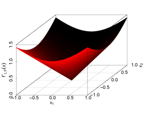
An essential theoretical task, which has attracted many considerations, is the investigation of learning rates for SVMs. For example, such rates for SVMs using the least squares loss and generic kernels can be found in (Cucker and Smale, 2002; De Vito et al., 2005; Smale and Zhou, 2007; Caponnetto and De Vito, 2007; Mendelson and Neeman, 2010; Steinwart et al., 2009) and the references therein, while similar rates for SVMs using the pinball loss can be found in (Steinwart and Christmann, 2008b, 2011). At this point, we do not want to take a closer look at these results, instead we relegate to (Eberts and Steinwart, 2013), where a detailed discussion can be found. More important for our purposes is the fact that Eberts and Steinwart (2011, 2013) establish (essentially) asymptotically optimal learning rates for least squares SVMs (LS-SVMs) using Gaussian RBF kernels. More precisely, for a domain , with , a distribution on such that has a bounded Lebesgue density on , and for contained in the Sobolev space , , or in the Besov space , , respectively, the LS-SVM using Gaussian kernels learns for all with rate with a high probability. Although these rates are essentially asymptotically optimal, they depend on the order of smoothness of the regression function on the entire input space . That is, if the regression function is on some area of smoother than on another area, the learning rate is determined by the part of , where the regression function is least smooth (cf. Figure 1).
In contrast to this, it would be desirable to achieve a learning rate on every region of that corresponds with the order of smoothness of on this region. Therefore, one of our goals of this paper is to modify the standard SVM approach such that we achieve local learning rates that are asymptotically optimal. Our technique to achieve such local learning rates is a special local SVM approach. Local SVMs have been extensively investigated in the literature to speed-up the training time, see for instance, the early works (Bottou and Vapnik, 1992; Vapnik and Bottou, 1993). The basic idea of many local approaches is to a) split the training data and just consider a few examples near a testing sample, b) train on this small subset of the training data, and c) use the solution for a prediction w.r.t. the test sample. Here, many up-to-date investigations use SVMs to train on the local data set but, yet there are different ways to split the whole training data set into smaller, local sets. For example, Chang et al. (2010); Wu et al. (1999); Bennett and Blue (1998) use decision trees while in (Hable, 2013; Segata and Blanzieri, 2010, 2008; Blanzieri and Melgani, 2008; Blanzieri and Bryl, 2007a, b; Zhang et al., 2006) local subsets are built considering nearest neighbors. The latter approaches further vary, for example, Zhang et al. (2006); Blanzieri and Bryl (2007a); Hable (2013) consider different metrics w.r.t. the input space whereas Segata and Blanzieri (2008); Blanzieri and Melgani (2008); Blanzieri and Bryl (2007b) consider metrics w.r.t. the feature space. Nonetheless, the basic idea of all these articles is that an SVM problem based on training samples is solved for each test sample. Another approach using nearest neighbors is investigated in (Segata and Blanzieri, 2010). Here, -neighborhoods consisting of training samples and collectively covering the training data set are constructed and an SVM is calculated on each neighborhood. The prediction for a test sample is then made according to the nearest training sample that is a center of a -neighborhood. As for the other nearest neighbor approaches, however, the results are mainly experimental. An exception to this rule is (Hable, 2013), where universal consistency for localized versions of SVMs, or more precisely, a large class of regularized kernel methods, is proven. Another article presenting theoretical results for localized versions of learning methods is (Zakai and Ritov, 2009). Here, the authors show that a consistent learning method behaves locally, i.e. the prediction is essentially influenced by close by samples. However, this result is based on a localization technique considering only training samples contained in a neighborhood with a fixed radius and center when an estimate in is sought. Probably closest to our approach is the one examined in (Cheng et al., 2010) and (Cheng et al., 2007), where the training data is splitted into clusters and then an SVM is trained on each cluster. However, the presented results are only of experimental character.
In this article, we partition the input space according to a cover of with radius and build an SVM model for each partition cell. The following section is dedicated to the detailed description of this method. Section 3 then presents some theoretical results that enable the analysis of this new method. For example, we examine extensions and direct sums of RKHSs. At the end of Section 3, we finally present a first oracle inequality for the localized SVM. In Section 4, we focus on RKHSs using Gaussian RBF kernels and, in conjunction with that, we study some entropy estimates. After that, Section 5 concentrates on the least squares loss and introduces an oracle inequality and learning rates for our localized SVM method using Gaussian kernels. Moreover, a data-dependent parameter selection method is studied that induces the same rates. Section 6 then presents some experimental results w.r.t. the localized SVM technique. All proofs can be found in Section 7, and the appendix contains various tables displaying detailed results of our experiments.
2 Description of the Localized SVM Approach
In this section, we introduce some general notations and assumptions. Based on the latter we modify the standard SVM approach. Let us start with the probability measure on , where is non-empty and for some . Depending on the learning target one chooses a loss function , i.e. a function that is measurable. Then, for a measurable function , the -risk is defined by
and the optimal -risk, called the Bayes risk with respect to and , is given by
A measurable function with is called a Bayes decision function. For the commonly used losses such as the least squares loss treated in Section 5 the Bayes decision function is -almost surely -valued, since . In this case, it seems obvious to consider estimators with values in on . To this end, we now introduce the concept of clipping the decision function. Let be the clipped value of some at defined by
Then a loss is called clippable at if, for all , we have
Obviously, the latter implies
for all . In other words, restricting the decision function to the interval containing our labels cannot worsen the risk, in fact, clipping this function typically reduces the risk. Hence, we consider the clipped version of the decision function as well as the risk instead of the risk of the unclipped decision function. Note, this clipping idea does not change the learning method since it is performed after the training phase.
To modify the standard SVM approach (1), we assume that is a partition of such that for every . Obviously, this implies for all with and
Now, the basic idea of the approach developed in this paper is to consider for each set of the partition an individual SVM. To describe this approach in a mathematically rigorous way, we have to introduce some more definitions and notations. Let us begin with the index set
indicating the samples of contained in , as well as the corresponding data set
Moreover, for every , we define a (local) loss function by
| (2) |
where is the loss that corresponds to our learning problem at hand. We further assume that is an RKHS over with kernel . Note that every function is only defined on even though a function is finally sought. To this end, for , we define a function by
Then the space equipped with the norm
is an RKHS on (cf. Lemma 2). That is, is an isometrically isomorphic extension of the RKHS on to an RKHS on . After all, we are now able to formulate a modified SVM approach. To this end, for every , consider the local SVM optimization problem
| (3) |
where for every . Based on these empirical SVM solutions, we then define the decision function by
| (4) |
where . Here, clipping at yields
for every . Note that the empirical SVM solutions in (3) exist and are unique by (Steinwart and Christmann, 2008a, Theorem 5.5) and that, for arbitrary , if for all . In addition, the SVM optimization problem (3) equals the SVM optimization problem (1) using , , and the regularization parameter , since, for and , we have
That is, as in (3) and satisfy
For the sake of completeness, we briefly examine the Bayes risks w.r.t. and . To this end, let , , be a loss function and be a distribution on such that a Bayes decision function exists. Then, for all and losses defined by (2), it is easy to show
whenever exists. In other words, a Bayes decision function w.r.t. and additionally is a Bayes decision function w.r.t. and . Moreover, for function spaces over , we have
| (5) |
by the construction of the loss .
Let us now present an advantageous characteristic of our modified SVM, namely the required computing time. Solving an usual SVM problem has a computational cost of where and is the sample size. For the new approach we consider working sets of size where for all , i.e. . Then for each working set an usual SVM problem has to be solved such that, altogether, the modified SVM induces a computational cost of . That is, for some and our approach is computationally cheaper than a traditional SVM. Note that our strategy using a partition of the input space is a typical way to speed-up algorithms and handle large data sets. Other techniques that possess similar properties are e.g. applied in the articles cited in the introduction. Besides, we refer to (Tsang et al., 2007) and (Tsang et al., 2005) using enclosing ball problems to solve an SVM, to (Graf et al., 2005) presenting an model of multiple filtering SVMs and to (Collobert et al., 2001) investigating a mixture of SVMs based on several subsets of the training set.
To describe the above SVM approach only has to be some partition of . However, for the theoretical investigations concerning learning rates of our new approach, we have to further specify the partition. To this end, we denote by the closed unit ball in the -dimensional Euclidean space and we define balls with radius and mutually distinct centers by
| (6) |
where is the Euclidean norm in . Moreover, choose and such that
i.e. such that the balls cover (cf. Figure 3). The following well-known lemma relates the radius of such a cover with the number of centers.
Lemma 1
Let be a bounded subset, i.e. for some constant . Then there exist balls with radius covering such that
For simplicity of notation, we assume in the following that , i.e. according to Lemma 1 there exists a cover with
| (7) |
Finally, we can specify the partition of by the following assumption.
-
(A)
Let be a partition of such that for every and such that there exist mutually distinct with , where is a cover of satisfying (7).
In the remaining sections we will frequently refer to Assumption (A). However, the results hold as well if we merely assume instead of in (A). The following example illustrates that (A) is indeed a natural assumption.
Example 1
For some , let us consider an -net of , where are mutually distinct. Based on these , a Voronoi partition of is defined by
| (8) |
cf. Figure 3. That is, contains all such that the center is the nearest center to , and if there exist and with and
for all , then since . In other words, they are resolved in favor of the smallest index of the involved centers. Moreover, it is obvious that , for all , for all with , and . In other words, a Voronoi partition based on an -net of satisfies condition (A), if and fullfil (7).
Following Example 1, we call the learning method producing given by (4) a Voronoi partition support vector machine, in short VP-SVM. Nevertheless, we just take a partition satisfying (A) as basis here instead of requesting to be a Voronoi partition.
Recall that our goal is to derive not only global but also local learning rates for this VP-SVM approach. To this end, we additionally consider an arbitrary measurable set such that . Then we examine the learning rate of the VP-SVM on this subset of . To formalize this, it is necessary to introduce some basic notations related to . Let us define the index set by
| (9) |
specifying every set that has at least one common point with . Note that, for every non-empty set , the index set is non-empty, too, i.e. . Besides, deriving local rates on requires us to investigate the excess risk of the VP-SVM with respect to the distribution and the loss defined by
| (10) |
However, to manage the analysis we additionally need the loss given by
| (11) |
which may only be nonzero, if is contained in some set with . Note that the risiks and quantify the quality of some function just on and
respectively. Hence, examining the excess risks
leads to learning rates on and implicitly on . Recapitulatory, let us declare a second set of assumptions.
- (T)
3 An Oracle Inequality for VP-SVMs
In this section, we first focus on RKHSs and direct sums of RKHSs. Then we present a lemma that relates the risk of a function w.r.t. the general loss to the risks w.r.t. the losses . Finally, we establish a first oracle inequality for VP-SVMs.
Let us begin with some basic notations. For and a measure , we denote by the Lebesgue spaces of order w.r.t. and for the Lebesgue measure on we write . In addition, for a measurable space , the set of all real-valued measurable functions on is given by . Moreover, for a measure on and measurable , we define the trace measure of in by for every .
Our first goal is to show that in (4) is actually an ordinary SVM solution. To this end, we consider an RKHS on some and extend it to an RKHS on by the following lemma, where we omit the obvious proof.
Lemma 2
Let and be an RKHS on with corresponding kernel . Denote by the extension of to defined by
Then the space equipped with the norm
is an RKHS on and its reproducing kernel is given by
| (12) |
Based on this lemma, we are now able to construct an RKHS by a direct sum of RKHSs and with and . Here, we skip the proof once more, since the assertion follows immediately using, for example, orthonormal bases of and .
Lemma 3
For such that and , let and be RKHSs of and over and , respectively. Furthermore, let and be the RKHSs of all functions of and extended to in the sense of Lemma 2 and let and given by (12) be the associated reproducing kernels. Then and hence the direct sum
| (13) |
exists. For and , let and be the unique functions such that . Then we define the norm by
| (14) |
and equipped with the norm is again an RKHS for which
is the reproducing kernel.
To relate Lemmas 2 and 3 with (4), we have to introduce some more notations. For pairwise disjoint sets , let be an RKHS on for every . Then, based on RKHSs on defined by Lemma 2, the joined RKHSs can be designed analogously to Lemma 3. That is, for an arbitrary index set and a vector , the direct sum
is again an RKHS equipped with the norm
| (15) |
If we simply write
| (16) |
Note that contains inter alia given by (4). Summarizing, we can define another assumption set.
- (H)
Having designed a joined RKHS as above, a crucial property of its function’s risks is expressed by the following lemma.
Lemma 4
Let be a distribution on and be a loss function. For such that and , define loss functions by and , respectively. Furthermore, let as well as be measurable functions and be defined by for all . Then we have
as well as
Note that Lemma 4 can be transferred to finite, pairwise disjoint unions. To be more precise, let us consider an arbitrary index set and define the corresponding loss function by
Now, it is straightforward to show
for every function . Based on this generalization and the whole index set , let us briefly consider Lemma 4 for the empirical measure and for , where , , are defined by (3). Then, for an arbitrary , it immediately follows
| (17) |
That is, is the decision function of an SVM using and as well as the regularization parameter . In other words, the latter SVM equals the VP-SVM given by (4). This will be a key insight used in our analysis.
To derive an oracle inequality, i.e. an appropriate upper bound for the excess risk for some index set , we have to introduce a few more notations. Let be a distribution on such that a Bayes decision function exists, for some constant at which can be clipped. Moreover, we denote by the function . If there exist constants , , and such that we have
| (18) | ||||
| (19) |
for all , , and , we say that the supremum bound (18) and the variance bound (19), respectively, is fulfilled. Actually, (18) immediately yields
for all and , i.e. the supremum bound is also satisfied for . Moreover, if (19) holds for all , the variance bound using the loss is satisfied, too. Indeed, by the use of for all , we have
for all . Let us quickly define a third assumption set.
-
(P)
Let be a distribution on such that the variance bound (19) is satisfied for constants , , and all functions .
Up to now, there is still missing a classical tool that is used to derive learning rates, namely entropy numbers, see (Carl and Stephani, 1990) or (Steinwart and Christmann, 2008a, Definition A.5.26). Recall that, for normed spaces and as well as an integer , the -th (dyadic) entropy number of a bounded, linear operator is defined by
where we use the convention , and as well as denote the closed unit balls in and , respectively. Finally, we present a first oracle inequality involving an upper bound for the excess risk , where is an arbitrary index set.
Theorem 5
Let be a locally Lipschitz continuous loss that can be clipped at and that satisfies the supremum bound (18) for some . Based on a partition of , where for every , we assume (H). Furthermore, for an arbitrary index set , we suppose (P). Assume that, for fixed , there exist constants and such that for all
| (20) |
Finally, fix an and a constant such that . Then, for all fixed , , and
the VP-SVM given by (4) using and satisfies
with probability not less than , where is a constant only depending on , , , , and .
The above theorem deals with the case of a partition with quite a few sets , . However, if we consider a partition consisting of just one set , i.e. , Theorem 5 is supposed to provide an oracle inequality that is comparable to the already known ones. To make that sure, let us briefly consider the case and hence , as well as RKHSs over X with . Note that in this case we have . If (20) holds for , Theorem 5 yields that an SVM using and satisfies
with probability not less than for fixed . Note that this oracle inequality indeed matches with the one stated in (Steinwart and Christmann, 2008a, Theorem 7.23) apart from the constant , which is, however, only depending on , , and .
4 Entropy Estimates for Local Gaussian RKHSs
In this section, we refine assumption (20). More precisely, in the subsequent theorem we determine an upper bound for the entropy numbers of the operator , where is the RKHS over of the Gaussian RBF kernel on defined by
for some width .
Theorem 6
Let , be a distribution on and be such that and such that there exists an Euclidean ball with radius containing , i.e. . Moreover, for , let be the RKHS of the Gaussian RBF kernel over . Then, for all , there exists a constant such that
Obviously, this theorem specifies assumption (20). Now, for the Gaussian case we elaborate assumption (H) and introduce the following additional set of assumptions.
- (G)
5 Learning Rates for Least Squares VP-SVMs
In this section, the non-parametric least squares regression problem is considered using the least squares loss defined by . It is well known that, in this case, the Bayes decision function is given by for -almost all . Moreover, this function is unique up to zero-sets. Besides, for the least squares loss the equality
can be shown by some simple, well-known transformations. Recall that is a non-empty subset of , where the index set defined by (9) indicates every set of the partition of that shares at least one point with . The associated loss function is defined by (11).
5.1 Basic Oracle Inequalities for LS-VP-SVMs
To formulate oracle inequalities and derive rates for VP-SVMs using the least squares loss, the target function is assumed to satisfy certain smoothness conditions. To this end, we initially recall the modulus of smoothness, a device to measure the smoothness of functions (see e.g. (DeVore and Lorentz, 1993, p. 44), (DeVore and Popov, 1988, p. 398), and (Berens and DeVore, 1978, p. 360)). Denote by the Euclidean norm and let be a subset with non-empty interior, be an arbitrary measure on , , and be contained in . Then, for , the -th modulus of smoothness of is defined by
where denotes the -th difference of given by
for and . Based on the modulus of smoothness, we introduce Besov spaces, i.e. function spaces that provide a finer scale of smoothness than the commonly used Sobolev spaces and that will thus be assumed to contain the target function later on. To this end, let , , , and be an arbitrary measure. Then the Besov space is defined by
where the seminorm is given by
or
see e.g. (Adams and Fournier, 2003, Section 7) and (Triebel, 2010, Sections 2 and 3). Note that actually describes a norm of for all , see e.g. (DeVore and Lorentz, 1993, pp. 54/55) and (DeVore and Popov, 1988, p. 398). Again, if is the Lebesgue measure on , we write . For the sake of completeness, recall from e.g. (Adams and Fournier, 2003, Section 3) and (Triebel, 2010, Sections 2 and 3) the scale of Sobolev spaces defined by
where , , is an arbitrary measure, and is the -th weak derivative for a multi-index with . That is, is the space of all functions in , whose weak derivatives up to order exist and are contained in . Moreover, the Sobolev space is equipped with the Sobolev norm
(cf. Adams and Fournier, 2003, page 60). We write and, for the Lebesgue measure on , we define . It is well-known, see e.g. (Edmunds and Triebel, 1996, p. 25 and p. 44), that the Sobolev spaces fall into the scale of Besov spaces, namely
for , , and . Moreover, for we actually have equality, that is with equivalent norms.
Based on the least squares loss and RKHSs using Gaussian kernels over the partition sets , the subsequent theorem refines the oracle inequality stated in Theorem 5.
Theorem 7
Let for , be the least squares loss and be a distribution on . We write . Furthermore, let (A) and (G) be satisfied. In addition, for an arbitrary subset , we assume (T). Moreover, let be a Bayes decision function such that as well as for some . Then, for all , , , , and , the VP-SVM given by (4) using , and the loss satisfies
with probability not less than , where is a constant only depending on , , , , , , and .
Using this oracle inequality, we derive learning rates w.r.t. the loss for the learning method described by (3) and (4) in the following theorem.
Theorem 8
Let be fixed and . Under the assumptions of Theorem 7 and with
| (21) | ||||
| (22) | ||||
| (23) |
for every , we have, for all and ,
with probability not less than , where as well as and are positive constants with .
In the latter theorem the condition is required to ensure , , which in turn is a prerequisite arising from Theorem 6 and the used entropy estimate. Let us briefly examine the extreme case . Using and (7) leads to covering numbers of the form and computational costs of which is actually less than the computational cost of order , , of an usual SVM. Note that for increasing the computational cost of an VP-SVM is increasing as well. However, for , , and , a VP-SVM has costs of which still is less that .
Let us finally take a closer look at the VP-SVM given by (4) and the considerations related to (17), where solves the minimization problem
Choosing , the VP-SVM problem can be understood as -multiple kernel learning (MKL) problem using the RKHSs . Learning rates for MKL have been treated, for example, in (Suzuki, 2011) and (Kloft and Blanchard, 2012). Assuming , the learning rate achieved in (Suzuki, 2011) is for dense settings, where is the so-called spectral decay coefficient. In addition, Kloft and Blanchard (2012) obtain essentially the same rates under these assumptions. Let us therefore briefly investigate the above rate of (Suzuki, 2011). For RKHSs that are continuously embedded in a Sobolev space , we have such that the learning rate reduces to . Note that this learning rate is times the optimal learning rate , where the number of kernels may increase with the sample size . In particular, if polynomially, then the rates obtained in (Suzuki, 2011) become substantially worse than the optimal rate. In contrast, due to the special choice of the RKHSs, this is not the case for our VP-SVM problem, provided that does not grow faster than .
Note that the oracle inequalities and learning rates achieved in Theorems 7 and 8 require . However, for an increasing sample size , the sets shrink and the index set , indicating every set such that and , increases. In particular, this also involves that the set covering changes in tandem with . Since this is very inconvenient and since it would be desirable to assume a certain level of smoothness of the target function on a fixed region for all , we consider the set enlarged by an -tube. To this end, for , we define by
| (24) |
which implies , cf. Figure 5. Note that, for every , there exists an such that for every the union of all partition sets , having at least one common point with , is contained in , i.e.
| (25) |
where . Collectively, this implies
for all . Furthermore, since every set is contained in a ball with radius , the lowest sample size in (25) can be determined by choosing the smallest such that with as in (7), that is
This leads to the following corollary where we present an oracle inequality and learning rates assuming the smoothness level of the target function on a fixed region.
Corollary 9
Let for , be the least squares loss, and be a distribution on . We write . Furthermore, let (A) and (G) be satisfied. In addition, for an arbitrary subset , we assume (T). Moreover, let be a Bayes decision function such that as well as
for and some . Then, for all , , , , and , the VP-SVM given by (4) using , and the loss satisfies
with probability not less than , where is the same constant as in Theorem 7.
Note that the assumption made in Corollary 9 is satisfied if, for example, and has a bounded Lebesgue density on . Moreover, if this density is even bounded away from 0, it is well-known that the minmax rate is for and target functions . Modulo , our rate is therefore asymptotically optimal in a minmax sense on . In addition, for , the learning rates obtained for are again asymptotically optimal modulo on .
5.2 Data-Dependent Parameter Selection for VP-SVMs
Note that in the previous theorems the choice of the regularization parameters and the kernel widths requires us to know the smoothness parameter . Unfortunately, in practice, we usually do know neither this value nor its existence. In this subsection, we thus show that a training/validation approach similar to the one examined in (Steinwart and Christmann, 2008a, Chapters 6.5, 7.4, 8.2) and (Eberts and Steinwart, 2013) achieves the same rates adaptively, i.e. without knowing . For this purpose, let and be sequences of finite subsets and . For a data set , we define
where and . We further split these sets in data sets
and define for all such that . For every , we basically use as a training set, i.e. based on in combination with the loss function we compute SVM decision functions
Again, note that if . Next, for each , we use in tandem with (or essentially ) to determine a pair such that
Finally, combining the decision functions for all , and defining and , we obtain a function
and we call every learning method that produces these resulting decision functions a training validation Voronoi partition support vector machine (TV-VP-SVM) w.r.t. . Moreover, using (5) we have, for and ,
where with for all . In other words, the function really minimizes the empirical risk w.r.t. the validation data set and the loss , where the minimum is taken over all functions with .
The following theorem presents learning rates for the above described TV-VP-SVM.
Theorem 10
Let with constants and . Under the assumptions of Theorem 7 we fix sequences and of finite subsets and such that is an -net of and is a -net of with and . Furthermore, assume that the cardinalities and grow polynomially in . Then, for all , , and , the TV-VP-SVM producing the decision functions satisfies
where is a constant independent of and .
Once more, we can replace the assumption by for some and obtain the same learning rate as in Theorem 10 for all although is fixed for all . Note that, if has a Lebesgue density that is bounded away from and and either for or for , these learning rates are again asymptotically optimal modulo on in a minmax sense. However, the condition restricts the set of -values where we obtain learning rates adaptively. To be more precise, there is a trade-off between and . On the one hand, for small values of only a small number of possible values for is covered. On the other hand, for larger values of the set of -values where we achieve rates adaptively is increasing but the savings in terms of computing time is decreasing.
6 Experimental Results
In the previous sections we defined VP-SVMs and derived local learning rates that are essentially optimal. So far, it is, however, not clear if the theoretical results suggesting a generalization performance not worse than that of global SVMs can be empirically confirmed and if the predicted advantages of VP-SVMs in terms of computational costs are preserved in practice. Note that the latter is not as obvious as it may seem to be, since VP-SVMs create an overhead when generating the working sets, and the working sets themselves do not need to be as balanced as we assumed in our naïve analysis. In this section, we thus investigate the performance of VP-SVMs empirically. Namely, we carry out some experiments using the least squares loss with the objective to answer the subsequent questions:
-
(1)
How do different radii affect the performance of VP-SVMs? In particular, what is the impact on the training time and the VP-SVM’s test error?
-
(2)
How do the VP-LS-SVMs perform compared to the usual LS-SVMs in terms of the test error? What is the speed-up?
-
(3)
How does the performance of VP-SVMs compare to vanilla data splitting approaches such as random chunking (RC-SVM), in which the data set is devided into a random partition with equally sized subsets, and the final decision function is the average of the SVMs computed on each subset?
-
(4)
How does the VP-LS-SVM behave compared to the global LS-SVM, if the regression function has interruptions of its smoothness on zero sets?


To address these questions we utilize two kinds of data sets. On the one hand, to answer questions (1), (2), and (3), we examine the three real data sets covtype, ijcnn1, and cod-rna, which we obtained from LIBSVM’s homepage, see (Chang and Lin, 2011). Table 1 summarizes some characteristics of these data sets.
| data set type | full data set size | dimension | number of labels |
|---|---|---|---|
| covtype | |||
| cod-rna | |||
| ijcnn1 |
On the other hand, we generated several artificial data sets to address the last question. In order to prepare the data sets for the experiments, we edited the data sets from LIBSVM in the following manner. If for a real-world data set type the raw data set was already split, we first merged these sets so that we obtained one data set for each data set type. In a next step, we scaled the data componentwise such that all samples including labels lie in , where is the dimension of the input data. Finally, for each data set type, we generated random subsets that were afterwards randomly splitted into a training and a test data set. In this manner, we obtained, for each of the three LIBSVM data set types, training sets consisting of samples. Additionally, for the data sets covtype and cod-rna, we created training sets of sizes and , and of sizes and , respectively. The test data sets associated to the various training sets consist of random samples, apart from the training sets with , for which we took test samples.
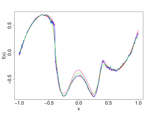
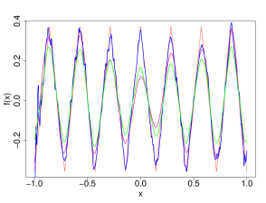
For the artificial data, we proceeded in a slightly different way. To generate the data sets we took as fundament the five regression functions pictured in Figure 6 and as noise, the sum of two uniform distributions on , where for the one-dimensional data sets and for the two-dimensional data sets. Thus, we produced five different types of artificial data sets, where the various data set types are named according to their type numbers as in Figure 6. Initially, we created two sets, namely one training and one test data set, each consisting of random input samples contained in and , respectively. Then, for each artificial data set type, we determined the labels belonging to the input data as sum of the corresponding functional value and the noise and, finally, scaled all labels to . In a last step, we randomly built subsets of the training sets of size . In this way, we altogether obtained, for each type of artificial data, four training data sets of size and a corresponding test data set of size . Based on the test data sets the Bayes risks can be determined, see Table 6 where the Bayes risks are summarized for the various artificial data set types.
| Type I | Type II | Type III | Type IV | Type V | |
| Bayes risk | 0.0254 | 0.0137 | 0.0529 | 0.0083 | 0.0634 |
To minimize random effects, we repeated the experiment for each setting several times. Since experiments using large data sets entail long run times, we reran every experiment using a training set of size only three times while for training sets of size we performed ten repetitions and for smaller training sets, namely of size , even runs. An exception are the experiments using artificial training sets of size , where we realized repetitions for the sake of uniformity.
To approach the above problems we used the least squares loss and Gaussian kernels for all experiments. We implemented an LS-SVM-solver in C++ similar to the one in (Steinwart et al., 2011). Around this solver, we then built the routines for the VP-SVM and the RC-SVM. The compilation of the three programmes was executed by LINUX’s gcc. To produce comparable results in terms of run time, all real-world data experiments were realized by the same professional compute server111On this occasion, we would like to thank the Institute for Applied Analysis and Numerical Simulation of the University of Stuttgart, who placed the above mentioned compute server at our disposal and, thus, enabled us to realize our experiments on large real-world data sets. In consequence, the overall time available for our experiments was limited. equipped with four INTEL XEON E7-4830 (2.13 GHz) 8-core processor, 256 GB RAM, and a 64 bit version of Debian GNU/Linux 6.0.7. In order that we can indeed compare their run time, we used eight cores to pre-compute the kernel matrix and to evaluate the final decision functions on the test set, and one core for the subsequent solver for every real data experiment. Since the artificial data sets consist of at most samples we performed the according experiments by a computer equipped with one INTEL CORE i7-3770K (3.50 GHz) quad core processor, 16 GB RAM, and a 64 bit version of Debian GNU/Linux 6.0.7. For all artificial data experiments we used four cores to pre-compute the kernel matrix and to evaluate the final decision functions on the test set, and again one core for the solver. Even with pre-computed kernel matrices, our experiments on the real-world data altogether required almost 810 hours (approximately 34 days) for training and additionally almost 4 days for testing. Moreover, the experiments on the artificial data took nearly 43 hours for training and 168 minutes for testing. Without pre-computing the kernel matrices, e.g. by applying a standard caching approach, preliminary experiments suggested a multiplcation of the training time, which would have rendered the experiments infeasible. Besides, our experiments will show that the available amount of RAM does not restrict the size of the training sets used by an VP-SVMs as severely as the ones used by LS-SVMs.
Let us quickly illustrate the routines of the VP- and the RC-SVM implemented around the LS-solver. For the VP-SVM, we first split the training set by Algorithm 1 in several working sets representing a Voronoi partition w.r.t. the user-specified radius. For this purpose, Algorithm 1 initially determines a cover of the input data applying the farthest first traversal algorithm, see (Dasgupta, 2008) and (Gonzalez, 1985) for more details. Note that this procedure induces working sets whose sizes may be considerably varying. In the case of an RC-SVM the working sets are created randomly, where their sizes are basically equal and the number of working sets is predefined by the user. Then, for the VP-SVM- as well as for the RC-SVM-algorithm the implemented LS-solver is applied on every working set. For each working set, we randomly split the respective training data set of size in five folds to apply 5-fold cross-validation in order to deal with the hyper-parameters and taken from an by grid geometrically generated in . Finally, we obtain one decision function for each working set. To further process these decision functions the VP-SVM-algorithms picks exactly one decision function depending on the working set affiliation of the input value. On the contrary, the RC-SVM-algorithm simply takes the average of all the decision functions. Moreover, since we scaled the labels of all data sets to , the computed decision functions are clipped at . Altogether, note that the usual LS-SVM-algorithm can be interpreted as special case of both the VP-SVM- and the RC-SVM-algorithm using one working set.
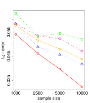
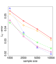
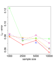
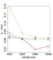
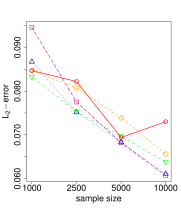
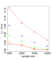
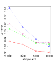
The experimental results for the three real data sets are summarized in Tables 7.3 to 7.3. These tables as well as Tables 7.3 to 7.3, containing the results for the experiments on the artificial data sets, can be found in the Appendix. In addition to the average run times of the training and test phases, these tables reflect inter alia the average test errors of the empirical SVM solutions. Additionally, the -errors of the empirical SVM solutions, i.e. the value of
is determined for the artificial data sets. Moreover, note that some of the result tables are incomplete for very large real-world training data sets. In these cases, the kernel matrix, whose size depends on the training set size, did not fit into the RAM of the used computer and, thus, these experiments were left out.
6.1 Experiments on Real-World Data
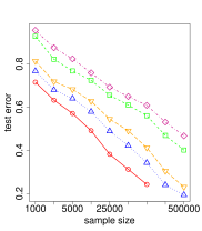
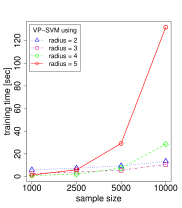
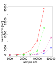
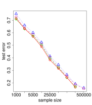
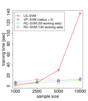
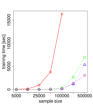
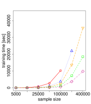
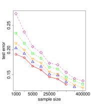
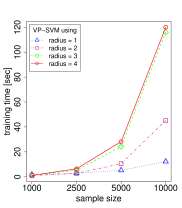
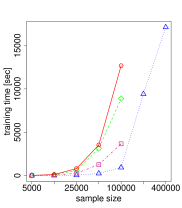
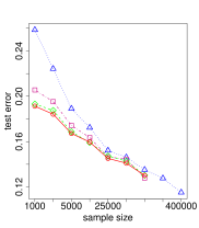
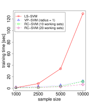
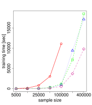
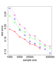
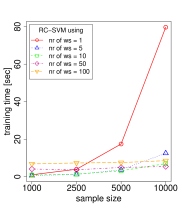
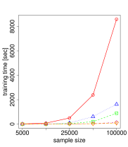
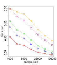
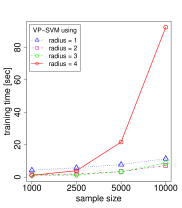
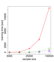
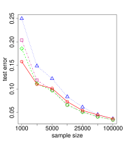
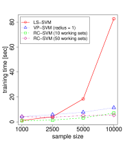
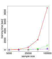
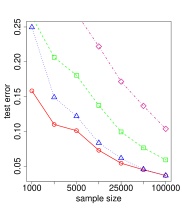
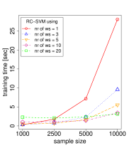
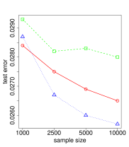
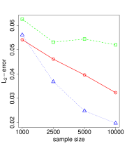
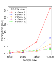
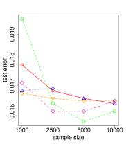
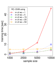
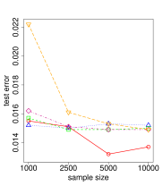
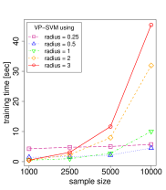
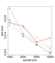
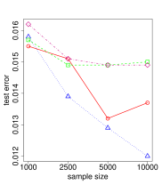
In this subsection, we adress questions (1), (2), and (3) by examining the results for the real-world data sets covtype, cod-rna, and ijcnn1, which are composed in Figures 6–6 and Tables 7.3–7.3.
6.1.1 Comparison of VP-SVMs Using Different Radii
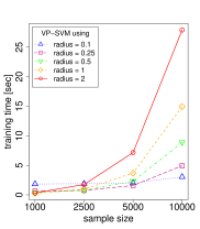
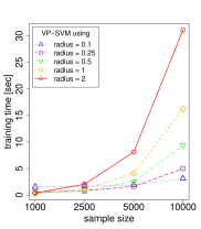
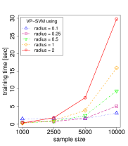
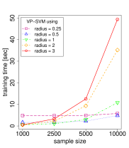
In the following, we focus on the VP-SVMs using four different radii for the various real-world data sets, where the experimental results are summarized in Tables 7.3–7.3 as well as in Subfigures 7(d)–7(f) of Figures 6–6. Examining the achieved training times for each data set type, we observe that, for increasing training set sizes, the radius that leads to the shortest training time typically decreases. More precisely, for the real data sets with sample size , the VP-SVMs using the smallest radius always train fastest, while for the data sets with , we can not make a uniform statement. Clearly, this finding is not surprising, since an SVM for a small data set trains considerably faster than an SVM for a large data set, such that splitting the large data set and running an SVM for each of the small data sets may altogether still be faster. Recall additionally the considerations in terms of the computational cost made in Section 2.
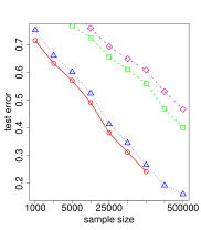
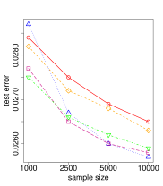
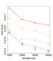
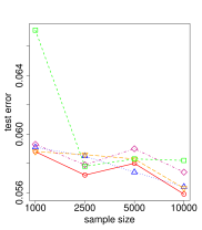
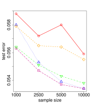
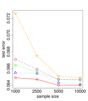
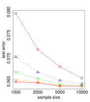
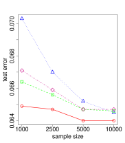
Let us now consider the VP-SVM results in terms of the realized test errors. As expected, for the real-world data sets, the test errors achieved by VP-SVMs with fixed radii decrease with increasing sample size of the used data sets except twice. In addition, for the real data sets covtype and cod-rna, the test errors decrease for increasing radii, cf. Figures 7(f) and 8(f). Here, however, the test errors achieved for the various radii get close to each other with increasing training sample size. The same behavior of the test errors appears for the ijcnn1 data set, though, for , both intermediate radii yield even smaller empirical risks than the largest radius, see Figure 9(f). In consequence, it is not straightforward to draw any conclusion on the relation between radius and test error. Nonetheless, we can say that VP-SVMs using small radii enjoy test errors that are never significantly larger and somethimes even smaller than those of VP-SVMs using the largest of the applied radii.
Besides, Tables 7.3 and 7.3 or Figures 7(e),7(f) and 8(e),8(f) contain an additional finding. For large data sets, namely for the covtype data set of size or for the cod-rna data sets of size and , the VP-SVMs with large radii did not yield any solution, since they failed due to the technical requirements caused by the used computer. More precisely, in these cases, there was at least one working set such that its kernel matrix did not fit into the RAM any more. Fortunately, the working sets of VP-SVMs using smaller radii were small enough such that we still received an outcome. What is more, these VP-SVMs yielded a better empirical risk in partially less training time compared to VP-SVMs with large radii and training sample sizes that still allowed a successful performance. That is, using a small radius for the VP-SVM and a training set that is oversized for VP-SVMs with a larger radius reduces the test error. More precisely, a large training set is crucial for a small empirical risk, where the possibly arising computational restrictions can be eluded by a VP-SVM with an appropriate radius.
All in all, localized SVMs using some small radius lead in substantially less training time to either negligble worse or even better test errors than VP-SVMs with large radii, if the training sample size is adequate, i.e. . In addition, the real data sets with a large sample size demonstrate that VP-SVMs with small radii are able to conquer the technical restrictions caused by the used computer and thus yield a better empirical risk than VP-SVMs with bigger radii can attain at all.
6.1.2 Comparing VP-SVMs with Global LS-SVMs
In the following, we compare the results of the VP-SVM using different radii to the standard LS-SVM. For the real-world data sets cod-rna and ijcnn1, the VP-SVMs, based on the largest of the applied radii, use only one working set. Thus, they coincide with the standard LS-SVM modulo different values generated by the random number generator. To verify this fact, we compare for the real data sets cod-rna and ijcnn1 the results of the VP-SVMs using one working set to the results of the standard LS-SVMs, see Tables 7.3 and 7.3. Here, we note that the LS-SVM test errors typically decrease with increasing training sample size. The same holds for the VP-SVMs using one working set. Moreover, the latter VP-SVM and the LS-SVMs perform equally well in terms of training time and empirical risk, however, for the VP-SVMs train slower.
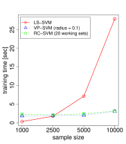
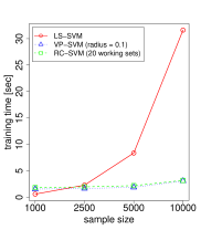
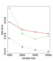
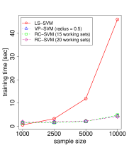
In practice, a crucial problem is caused by the run time required by an algorithm. Hence, for each data set type, we compare hereafter the LS-SVM to the VP-SVM that trains fastest for the largest training data set. The required average training times and the average test errors of these SVMs are illustrated in Subfigures 7(g)–7(i) of Figures 6–6. First, we notice that the selected VP-SVM uses the smallest of the applied radii for each data set type. Besides, the LS-SVM’s test errors are lower than those of the VP-SVMs. However, with increasing training set size the VP-SVM’s test errors get close to the ones of the LS-SVM. Moreover, for the ijcnn1 data set of size , their empirical risks even coincide, cf. Figure 9(i). Besides, the VP-SVMs train considerably faster than the LS-SVMs. In particular, for the VP-SVMs require at most of the LS-SVM’s training times, see Figures 7(h), 8(h), and 9(h). Finally, recall that, for data sets of size , the LS-SVM problem is infeasible with our computer, just like the VP-SVMs using the largest of the applied radii. In contrast, for , VP-SVMs using small radii usually train considerably faster and achieve lower test errors than the LS-SVMs for , cf. Figures 7(h)–7(i) and 8(h)–8(i).
Concluding, we have seen that the application of a VP-SVM using a small radius instead of the standard LS-SVM reduces the run time considerably entailing at most a negligible worsening or even an improvement of the test errors. Moreover, applying VP-SVMs with sufficiently small radii enables us to use large data sets and, thus, to elude the computational restrictions to sufficiently small data sets. As a result, handling really large data sets with the help of suitable VP-SVMs can lead to significantly improved test errors compared to an LS-SVM setting with memory constraints.
6.1.3 Comparison of VP-SVMs with RC-SVMs
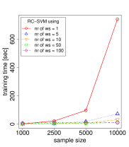
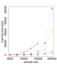
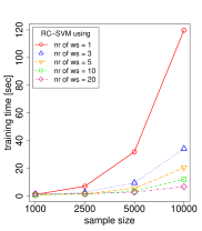
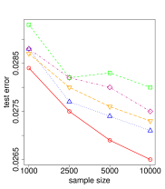
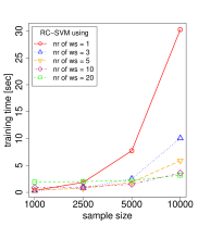
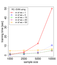
First of all, let us investigate the RC-SVM results that are composed in Tables 7.3–7.3 as well as in Subfigures 7(a)–7(c) of Figures 6–6. For the real data sets covtype we considered ten, for the data sets cod-rna nine, and for the data sets ijcnn1 eight different numbers of working sets. In each case, we started with an RC-SVM using one working set, i.e. with an RC-SVM that corresponds to the global LS-SVM modulo different values generated by the random generator, cf. Tables 7.3 and 7.3. Comparing for every data set the RC-SVMs using various numbers of working sets, we observe that the number of working sets, minimizing the RC-SVMs training time, increases in tandem with the sample size. Moreover, the RC-SVM using one working set never trains fastest compared to the other RC-SVMs using more than one working set. Furthermore, the average test errors for the applied RC-SVMs usually decrease for a decreasing number of working sets and, hence, are minimized by the smallest possible number of working sets. Of course, all these findings are not surprising, since RC-SVMs are typically used to reduce the training time.
Let us now compare the results of VP- and RC-SVMs using roughly the same number of working sets, cf. Tables 7.3–7.3. Initially note that, even though we consider VP- and RC-SVM based on the same number of working sets, the RC-SVM working sets are about the same size whereas the VP-SVM working sets may have different sizes with a large range. That is, the VP-SVMs often deal with a few substantially larger working sets than the RC-SVMs. Consequently, the RC-SVMs often perform faster than the VP-SVMs, which require up to five times the RC-SVM’s training time for . Contrarily, the average empirical risks achieved by the VP-SVMs are substantially lower than those of the RC-SVMs. Besides, in a few cases the VP-SVMs possess at least one working set which is oversized for the computer’s RAM, so that these VP-SVM problems are infeasible, whereas the comparable RC-SVMs avoid this conflict. Here, consider e.g. the RC-SVM using seven working sets and the VP-SVM with radius for the covtype data set of size .
In Section 6.1.2, we compared for each data set type the LS-SVM with the VP-SVM that trains fastest for the largest training data set. Here, we additionally compare this VP-SVM to the RC-SVMs. To be able to draw a fair comparison in terms of the achieved test errors, we choose those RC-SVMs that train roughly as fast as the VP-SVM for the largest training set, i.e. the slowest RC-SVM training faster and the fastest RC-SVM training slower than the above VP-SVM. Subfigures 7(g)–7(i) of Figures 6–6 illustrate the average training times and the average test errors of these RC-SVMs, the above VP-SVM, and the LS-SVM. Considering the RC-SVMs, the faster of the two requires for between and of the VP-SVMs training time and trains at most seven minutes faster than the VP-SVM. However, at least for , both considered RC-SVMs induce substantially higher test errors than the VP- and LS-SVM. Finally, note that VP-SVMs for considerably outperform LS-SVMs for , while RC-SVMs for lead to even worse test errors than the considered LS-SVMs.
Summarizing, we record that RC-SVMs using as few as possible working sets achieve the smallest RC-SVM test errors, however, those using more working sets perform faster. Furthermore, compared to VP-SVMs using roughly the same number of working sets as the RC-SVMs, the latter ones may learn faster though not as good as the VP-SVMs. Moreover, considering RC-SVMs that require roughly the same training time as the fastest VP-SVM, we saw that the RC-SVMs lead to much higher empirical risks. That is, if the required training time is a hard constraint, then the VP-SVM that satisfies this constraint achieves a better test error than a RC-SVM that also trains fast enough.
6.2 Experiments on Artificial Data

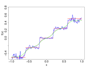
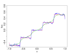
| Bayes decision function | |
| average empirical LS-SVM solution |
| average empirical VP-SVM solution | |
| average empirical RC-SVM solution |
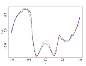
| Bayes decision function | |
| average empirical LS-SVM solution |
| average empirical VP-SVM solution | |
| average empirical RC-SVM solution |
| Bayes decision function | |
| average empirical LS-SVM solution |
| average empirical VP-SVM solution | |
| average empirical RC-SVM solution |
| Bayes decision function | |
| average empirical LS-SVM solution |
| average empirical VP-SVM solution | |
| average empirical RC-SVM solution |


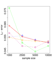
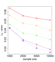
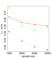
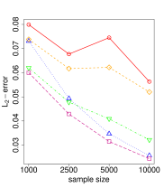
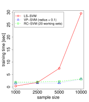
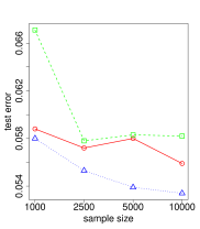
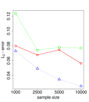
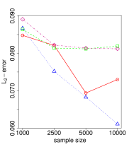
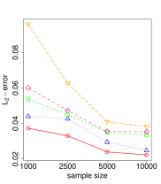
It remains to address the last question. To this end, we consider the results on the various artificial data sets, on the one hand, for the LS-SVM and, on the other hand, for the VP-SVM performing fastest for . Moreover, for the sake of comparability, we again add to this selection the two RC-SVMs training roughly as fast as the VP-SVM for the artificial data sets of size . However, for the artificial data sets of Type I, II, and III, none of the executed RC-SVMs trained faster for than the VP-SVM with the smallest radius, so that we only consider one RC-SVM in these cases. The required average training times and average test errors of the selected SVMs are illustrated in Subfigures 10(g)–10(i) of Figures 6–6 and summarized in Tables 7.3–7.3. Here, we note that, for the artificial data of Type I, II, and III, the VP-SVM using the smallest of the applied radii trains fastest for , while for the artificial data of Type IV and V it is the VP-SVM using the second smallest radius.
Expectedly, we detect an evident improvement of the various average empirical SVM solutions using training samples instead of samples. Besides, the considered VP-SVM trains substantially faster than the standard LS-SVM with less than of the LS-SVM’s training time for . Additionally, the VP-SVM’s test errors are usually considerably lower than the test errors of the LS-SVM. Regarding the test errors of the RC-SVMs, we note that, in the majority of cases, they are higher than the VP-SVM’s and the LS-SVM’s test errors.
So far, we examined the behavior of LS-, VP-, and RC-SVMs in terms of training time and test error. Let us finally compare the three different kinds of SVMs w.r.t. their optical appearance. To this end, the average empirical SVM solutions are plotted in Figures 15–6 for the different artificial data sets of size and . Here, note that, for the artificial data of Type IV and V, we do not consider both RC-SVMs training roughly as fast as the selected VP-SVM but only the one of the both RC-SVMs with the lower test error.
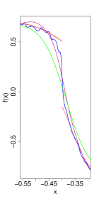
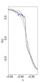
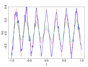
The observation that, for the artificial data of Type I, II, and III, the VP-SVMs perform best, is reinforced by the average empirical VP-SVM solutions illustrated in Figures 15–18. More precisely, Figure 15 shows that only the VP-SVMs exhaust the widths of the steps of almost completely. Moreover, in Figure 6 the smoothness interruptions of are again best illustrated by the VP-SVMs, which becomes even more evident in Figure 6. Besides, Figure 18 illustrates that the peaks of are best reproduced by the VP-SVMs. Considering the LS- and the RC-SVMs, we can not draw an universally valid conclusion, which one performs worse. In particular, Figures 15 and 6 show that, for the artificial data sets of Type I and II, both, the average empirical LS- and RC-SVM solutions, are not very well suited to the Bayes decision function. Considering the data sets of Type III, the LS-SVMs dominate the RC-SVMs in terms of the better test errors, though both kinds of SVMs do not reproduce the peaks of , especially for small values of .
It remains to optically analyze the results of the two-dimensional data sets in the following. For the artificial data sets of Type IV, the VP-SVM using training samples achieves the best test error. Moreover, ensuing the optical impression, this VP-SVM is the only one of the considered SVM types that reflects the circular steps of the Bayes decision function as in Figure 6(d), cf. Figure 6. Finally, for the data sets of Type V, it is always the LS-SVM which performs best in terms of the test errors, cf. Table 7.3. This observation is also substantiated optically. To be more precise, for , the uneven average empirical decision function induced by the VP-SVM (cf. Figure 6) shows that the RC-SVM even performs better than the VP-SVM. However, for , the VP-SVM results are substantially improved such that the RC-SVM is now outperformed by the VP-SVM.
Recapulatory, we realize that the VP-SVMs possess the most distinctive ability to handle smoothness interruptions of the Bayes decision function in most of our artificial data cases, especially if . For the sake of completeness, we point out that the worst performance was induced by the RC-SVMs in almost all cases, in particular for a training sample size amounting to .
6.3 Conclusions
Finally, we summarize the essential findings of the previous subsections, where we considered standard LS-SVMs and two kinds of localized SVMs, namely VP-SVMs and RC-SVMs. As just analyzed in Subsection 6.2, VP-SVMs have the evident advantage that they manage smoothness interruptions of the Bayes decision function better than LS- and RC-SVMs.
The real-world data sets demonstrated that the RC-SVMs perform considerably worse than the LS-SVMs and the VP-SVMs, while the performance of VP-SVMs using small radii is improved for increasing sample sizes. To be more precise, VP-SVMs outperform LS-SVMs or at most leads to a negligible worsening compared to LS-SVMs for a fraction of the training time and without memory constraints on the large data sets. For very small data sets, however, LS-SVMs actually train faster than VP-SVMs and, hence, are preferable. What is more, for data sets of size all LS-SVMs require less than 9s to train, so that there are probably no reasons to apply a VP-SVM. Besides, really small training sample sizes involve considerably smaller working sets for a VP-SVM using a small radius, so that it is hard to find a well suited prediction.
Furthermore, despite a faster training procedure, a VP-SVM using a sufficiently small radius induces considerably lower test errors for sample sizes than a LS-SVM for training data sets that still enable computational feasibility.
7 Proofs
This section is dedicated to prove the results of the previous sections. We begin with the proof of Lemma 1 relating the radius of a cover of defined by (6) with the number of centers .
Proof [Proof of Lemma 1] First of all, let us recall the -th entropy number of defined by
Since , the -th entropy number of can be upper bounded by
Additionally, we know by (Carl and Stephani, 1990, Section 1.1) that
so that we can find a cover of satisfying
7.1 Proofs of Section 3
In Section 3 we presented a lemma that related the risk w.r.t. the loss to the risk w.r.t. the restricted loss and also transferred this result to the excess risk. Hereafter, the proof of this lemma can be found.
Proof [Proof of Lemma 4] Simple transformations using and show
The second assertion follows immediately.
To derive the new oracle inequality of Theorem 5 we first have to relate the entropy numbers of , , to those of . To this end, we consider a similar concept to entropy numbers, namely covering numbers, cf. (Györfi et al., 2002, Definition 9.3) or (Steinwart and Christmann, 2008a, Definition 6.19).
Definition 11
Let be a metric space and . A subset is called an -net of if for all there exists an such that . Furthermore, we define the -covering number of by
where and .
Note that an upper bound on entropy numbers involves a bound on covering numbers. To be more precise, for a metric space and constants and , the implication
| (26) |
holds by (Steinwart and Christmann, 2008a, Lemma 6.21). Additionally, (Steinwart and Christmann, 2008a, Exercise 6.8) yields the opposite implication, namely
| (27) |
Recall that we pursue the target to estimate . In fact, the equivalence of entropy and covering numbers enables us to estimate the covering number of instead.
Lemma 12
Let be a distribution on and with . Moreover, let and be RKHSs on and that are embedded into and , respectively. Let the extended RKHSs and be defined as in Lemma 2 and denote their direct sum by as in (13), where the norm is given by (14) with . Then, for the -covering number of w.r.t. , we have
where and .
Proof First of all, we assume that there exist and functions and such that is an -cover of w.r.t. , is an -cover of w.r.t. ,
That is, for every function , there exists an such that
| (28) |
and for every function , there exists an such that
| (29) |
Let us now consider an arbitrary function . Then there exists an and an such that . Together with (28) and (29), this implies
With this, we know that
is an -net of w.r.t. . Concerning the -covering number of , this finally implies
Based on Lemma 12, the following theorem relates entropy numbers of and to those of .
Theorem 13
Let be a distribution on and be pairwise disjoint. Moreover, we assume (H) with weights . In addition, assume that there exist constants and , , such that for every
| (30) |
Then we have
and, for the average entropy numbers,
Proof [Proof of Theorem 13] First of all, note that the restriction operator with is an isometric isomorphism. Together with (Steinwart and Christmann, 2008a, (A.36)) and assumption (30), this yields
Furthermore, we know by (26) that
holds for all . With this and for every , Lemma 12 implies
Using (27), the latter bound for the covering number of finally implies the following entropy estimate
The second assertion immediately follows by (Steinwart and Christmann, 2008a, Corollary 7.31).
Applying Theorem 13, we now prove Theorem 5 and thus an oracle inequality for VP-SVMs using an ordinary type of losses.
Proof [Proof of Theorem 5] Since are seperable RKHS of mesurable kernels , is a seperable RKHS and its kernel is measurable, too. Furthermore, Theorem 13 yields
That is, we can apply (Steinwart and Christmann, 2008a, Theorem 7.23) for a regularization parameter and, for all fixed and , , we obtain
with probability not less than , where is the constant of (Steinwart and Christmann, 2008a, Theorem 7.23) only depending on , , , , and . Moreover,
where we need since it is a condition of (Steinwart and Christmann, 2008a, Theorem 7.23).
7.2 Proofs Related to the Entropy Estimates of Section 4
In this subsection, just as in Section 4, we focus on Gaussian RBF kernels and the associated RKHSs. To be more precise, we derive a bound for the entropy numbers of , where and with .
Proof [Proof of Theorem 6] First of all, we consider the commutative diagram
where the extension operator and the restriction operator given by (Steinwart and Christmann, 2008a, Corollary 4.43) are isometric isomorphisms, so that . Furthermore, for , we have
i.e. . Together with (Steinwart and Christmann, 2008a, (A.38) and (A.39)) as well as (Steinwart and Christmann, 2008a, Theorem 6.27), we obtain for all
where is an arbitrary integer and a positive constant. For , the choice finally yields
7.3 Proofs Related to the Least Squares VP-SVMs
In this subsection, we prove the results that are linked with the least squares loss, i.e. the results of Section 5. Before we elaborate on the oracle inequality for VP-SVMs using the least squares loss as well as RKHSs of Gaussian kernels, we have to examine the excess risk
| (31) |
Let us begin by writing for fixed
| (32) |
and choosing . Then (31) can be estimated with the help of the following theorem, which is together with its proof basically a modification of (Eberts and Steinwart, 2013, Theorem 2.2). Indeed, the proofs proceed mainly identically. Note that we use the notation
in the following theorem and the associated proof.
Theorem 14
Let us fix some . Assume that is a finite measure on with and let be a partition of . Furthermore, let be such that for some . For the functions , , defined by (32), where and , we then have
where .
Proof In the following, we write . To show
we have to proceed in a similar way as in the proof of (Eberts and Steinwart, 2013, Theorem 2.2). First of all, we use the translation invariance of the Lebesgue measure and () to obtain, for and ,
With this we can derive, for ,
Then Hölder’s inequality and yield, for ,
Moreover, for , we have
Consequently, we can proceed in the same way for all . To this end, note that the assumption implies for . The latter together with Hölder’s inequality yields
Using the embedding constant of to , we obtain
for . With the substitution , the functional equation of the Gamma function , and we further have
Altogether, we finally obtain
Proof [Proof of Theorem 7] First, we have to choose a function . To this end, we define functions , , by (32), where and . Then we define by convolving each with the Bayes decision function , that is
Now, to show that is indeed a suitable function to bound the approximation error, we first need to ensure that is contained in . In addition, we need to derive bounds for both, the regularization term and the excess risk of . To this end, we apply (Eberts and Steinwart, 2013, Theorem 2.3) and obtain, for every ,
with
This implies
Besides, note that for every such that can be written as , where
Obviously, the latter implies . Furthermore, for , (31) and Theorem 14 yield
where is a constant only depending on , , and . To utilize Theorem 5, it remains to examine the constants , and . Since we consider the least squares loss, which can be clipped at with , the supremum bound (18) holds for and the variance bound (19) for and (cf. Steinwart and Christmann, 2008a, Example 7.3). Next, we derive a bound for using (Eberts and Steinwart, 2013, Theorem 2.3) which provides, for every , the supremum bound
| (33) |
The latter implies
i.e. . Moreover, since Theorem 6 provides for with , we have
where we used the concavity of the function for , by (7), and . Finally, applying Theorem 5 yields
with probability not less than . Finally, for , a variable transformation implies
with probability not less than , where the constant is defined by
Next, using the just proven oracle inequality presented in Theorem 7, we show the learning rates of Theorem 8 in only a few steps.
Proof [Proof of Theorem 8] First of all, we define sequences and to simplify the presentation. Then Theorem 7, , and together with and for all yield
Using the choices , , as well as finally implies
with probability not less than , where is a constant and .
Proof [Proof of Corollary 9] For simplicity of notation, we write , , , and instead of , , , and . Since for all , the assumption implies
With this, Theorems 7 and 8 immediately yield
with probability not less than , where . Moreover, the constants and coincide with those of Theorems 7 and 8.
It remains to prove Theorem 10. However, we previously have to consider the following technical lemma.
Lemma 15
Let and with and a constant . We fix finite subsets and such that is an -net of and is an -net of with , , , and . Moreover, let be an arbitrary non-empty index set and . Then, for all , , and all with , we have
where and is a constant independent of , , , , and .
Proof Without loss of generality, we may assume that and are of the form and with and as well as and for all and . With and it is easy to see that
| (34) |
hold for all and . Furthermore, define and . Then there exist indices and with and . Together with (34), this yields
| (35) |
Moreover, the definition of implies and the one of implies for and , where . Additionally, it is easy to check that
| (36) |
where is a positive constant. Using (35), the bound , and (36), we obtain
with and constants and independent of , , , , and .
Proof [Proof of Theorem 10] Let be defined by , i.e. . With this, Theorem 7 yields with probability not less than that
| (37) |
for all , , simultaneously, where is a constant independent of , , , and . Furthermore, the oracle inequality of (Steinwart and Christmann, 2008a, Theorem 7.2) for empirical risk minimization, , and yield
| (38) | |||
| (39) |
with probability not less than . With (37), (39) and Lemma 15 we can conclude
with probability not less than . Finally, a variable transformation yields
with probability not less than , where we used
in the last step.
References
- Adams and Fournier (2003) R. A. Adams and J. J. F. Fournier. Sobolev Spaces. Academic Press, New York, 2nd edition, 2003.
- Aronszajn (1950) N. Aronszajn. Theory of reproducing kernels. Trans. Amer. Math. Soc., 68:337–404, 1950.
- Bennett and Blue (1998) K.P. Bennett and J. A. Blue. A support vector machine approach to decision trees. In Neural Networks Proceedings, 1998. IEEE World Congress on Computational Intelligence. The 1998 IEEE International Joint Conference on, volume 3, pages 2396–2401 vol.3, 1998. doi: 10.1109/IJCNN.1998.687237.
- Berens and DeVore (1978) H. Berens and R. DeVore. Quantitative Korovkin Theorems for Positive Linear Operators on - Spaces. Trans. Amer. Math. Soc., 245:pp. 349–361, 1978. ISSN 00029947. URL http://www.jstor.org/stable/1998871.
- Berlinet and Thomas-Agnan (2004) A. Berlinet and C. Thomas-Agnan. Reproducing Kernel Hilbert Spaces in Probability and Statistics. Kluwer, Boston, 2004.
- Blanzieri and Melgani (2008) E. Blanzieri and F. Melgani. Nearest Neighbor Classification of Remote Sensing Images With the Maximal Margin Principle. Geoscience and Remote Sensing, IEEE Transactions on, 46(6):1804–1811, 2008. ISSN 0196-2892. doi: 10.1109/TGRS.2008.916090.
- Blanzieri and Bryl (2007a) Enrico Blanzieri and Anton Bryl. Instance-based spam filtering using SVM nearest neighbor classifier. In In Proceedings of FLAIRS 2007, pages 441–442, 2007a.
- Blanzieri and Bryl (2007b) Enrico Blanzieri and Anton Bryl. Evaluation of the Highest Probability SVM Nearest Neighbor Classifier with Variable Relative Error Cost. In In Proceedings of Fourth Conference on Email and Anti-Spam, CEAS’2007, 2007b.
- Bottou and Vapnik (1992) Léon Bottou and Vladimir Vapnik. Local Learning Algorithms. Neural Computation, 4:888–900, 1992.
- Caponnetto and De Vito (2007) A. Caponnetto and E. De Vito. Optimal rates for regularized least squares algorithm. Found. Comput. Math., 7:331–368, 2007.
- Carl and Stephani (1990) B. Carl and I. Stephani. Entropy, Compactness, and the Approximation of Operators. Cambridge Tracts in Mathematics. Cambridge University Press, Cambridge, 1990. ISBN 9780521330114. URL http://books.google.de/books?id=xlBNHvgP7PIC.
- Chang and Lin (2011) Chih-Chung Chang and Chih-Jen Lin. LIBSVM: A library for support vector machines. ACM Transactions on Intelligent Systems and Technology, 2:27:1–27:27, 2011. Software available at http://www.csie.ntu.edu.tw/~cjlin/libsvm.
- Chang et al. (2010) Fu Chang, Chien-Yang Guo, Xiao-Rong Lin, and Chi-Jen Lu. Tree Decomposition for Large-Scale SVM Problems. J. Mach. Learn. Res., 11:2935–2972, December 2010. ISSN 1532-4435. URL http://dl.acm.org/citation.cfm?id=1756006.1953027.
- Cheng et al. (2007) Haibin Cheng, Pang-Ning Tan, and Rong Jin. Localized Support Vector Machine and Its Efficient Algorithm. In SIAM International Conference on Data Mining, 2007.
- Cheng et al. (2010) Haibin Cheng, Pang-Ning Tan, and Rong Jin. Efficient Algorithm for Localized Support Vector Machine. Knowledge and Data Engineering, IEEE Transactions on, 22(4):537–549, 2010. ISSN 1041-4347. doi: 10.1109/TKDE.2009.116.
- Collobert et al. (2001) Ronan Collobert, Samy Bengio, and Yoshua Bengio. A Parallel Mixture of SVMs for Very Large Scale Problems. In In Advances in Neural Information Processing Systems, pages 633–640, 2001.
- Cucker and Smale (2002) F. Cucker and S. Smale. On the mathematical foundations of learning. Bull. Amer. Math. Soc., 39:1–49, 2002.
- Dasgupta (2008) Sanjoy Dasgupta. Lecture 1: Clustering in metric spaces. CSE 291: Topics in unsupervised learning, 2008. URL http://cseweb.ucsd.edu/~dasgupta/291/lec1.pdf.
- De Vito et al. (2005) E. De Vito, A. Caponnetto, and L. Rosasco. Model selection for regularized least-squares algorithm in learning theory. Found. Comput. Math., 5:59–85, 2005.
- DeVore and Popov (1988) R.A. DeVore and V.A. Popov. Interpolation of Besov Spaces. Trans. Amer. Math. Soc., 305(1):pp. 397–414, 1988.
- DeVore and Lorentz (1993) Ronald Alvin DeVore and George G. Lorentz. Constructive Approximation. Grundlehren der mathematischen Wissenschaften. Springer-Verlag, Berlin, 1993. ISBN 3-540-50627-6. URL http://books.google.de/books?id=cDqNW6k7_ZwC.
- Eberts and Steinwart (2011) Mona Eberts and Ingo Steinwart. Optimal learning rates for least squares SVMs using Gaussian kernels. In J. Shawe-Taylor, R.S. Zemel, P. Bartlett, F.C.N. Pereira, and K.Q. Weinberger, editors, Advances in Neural Information Processing Systems 24, pages 1539–1547. 2011.
- Eberts and Steinwart (2013) Mona Eberts and Ingo Steinwart. Optimal regression rates for SVMs using Gaussian kernels. Electron. J. Statist., 7:1–42, 2013. ISSN 1935-7524. doi: 10.1214/12-EJS760.
- Edmunds and Triebel (1996) D. E. Edmunds and H. Triebel. Function Spaces, Entropy Numbers, Differential Operators. Cambridge University Press, Cambridge, 1996.
- Gonzalez (1985) Teofilo F. Gonzalez. Clustering to minimize the maximum intercluster distance. Theoretical Computer Science, 38(0):293–306, 1985. ISSN 0304-3975. doi: http://dx.doi.org/10.1016/0304-3975(85)90224-5. URL http://www.sciencedirect.com/science/article/pii/0304397585902245.
- Graf et al. (2005) Hans Peter Graf, Eric Cosatto, Leon Bottou, Igor Durdanovic, and Vladimir Vapnik. Parallel Support Vector Machines: The Cascade SVM. In In Advances in Neural Information Processing Systems, pages 521–528. MIT Press, 2005.
- Györfi et al. (2002) L. Györfi, M. Kohler, A. Krzyżak, and H. Walk. A Distribution-Free Theory of Nonparametric Regression. Springer-Verlag, New York, 2002.
- Hable (2013) Robert Hable. Universal consistency of localized versions of regularized kernel methods. J. Mach. Learn. Res., 14(1):153–186, January 2013. ISSN 1532-4435. URL http://dl.acm.org/citation.cfm?id=2502581.2502586.
- Kloft and Blanchard (2012) Marius Kloft and Gilles Blanchard. On the convergence rate of -norm multiple kernel learning. J. Mach. Learn. Res., 13:2465–2502, Aug 2012.
- Koenker (2005) R. Koenker. Quantile Regression. Econometric Society Monographs. Cambridge University Press, 1st edition, 2005. ISBN 9780521608275. URL http://books.google.de/books?id=hdkt7V4NXsgC.
- Mendelson and Neeman (2010) S. Mendelson and J. Neeman. Regularization in kernel learning. Ann. Statist., 38:526–565, 2010.
- Segata and Blanzieri (2008) Nicola Segata and Enrico Blanzieri. Empirical assessment of classification accuracy of local SVM. Technical report, University of Trento, Information Engineering and Computer Science, 2008. URL eprints.biblio.unitn.it/1398/1/014.pdf.
- Segata and Blanzieri (2010) Nicola Segata and Enrico Blanzieri. Fast and Scalable Local Kernel Machines. J. Mach. Learn. Res., 11:1883–1926, August 2010. ISSN 1532-4435. URL http://dl.acm.org/citation.cfm?id=1756006.1859915.
- Simonoff (1996) J. S. Simonoff. Smoothing Methods in Statistics. Springer, New York, 1996.
- Smale and Zhou (2007) S. Smale and D.-X. Zhou. Learning theory estimates via integral operators and their approximations. Constr. Approx., 26:153–172, 2007.
- Steinwart and Christmann (2008a) I. Steinwart and A. Christmann. Support Vector Machines. Springer, New York, 2008a.
- Steinwart and Christmann (2008b) I. Steinwart and A. Christmann. How SVMs can estimate quantiles and the median. In J.C. Platt, D. Koller, Y. Singer, and S. Roweis, editors, Advances in Neural Information Processing Systems 20, pages 305–312, Cambridge, MA, 2008b. MIT Press.
- Steinwart and Christmann (2011) I. Steinwart and A. Christmann. Estimating conditional quantiles with the help of the pinball loss. Bernoulli, 17:211–225, 2011.
- Steinwart et al. (2009) I. Steinwart, D. Hush, and C. Scovel. Optimal rates for regularized least squares regression. In S. Dasgupta and A. Klivans, editors, Proceedings of the 22nd Annual Conference on Learning Theory, pages 79–93, 2009.
- Steinwart et al. (2011) I. Steinwart, D. Hush, and C. Scovel. Training SVMs without offset. J. Mach. Learn. Res., 12:141–202, 2011.
- Suzuki (2011) Taiji Suzuki. Unifying Framework for Fast Learning Rate of Non-Sparse Multiple Kernel Learning. In J. Shawe-Taylor, R.S. Zemel, P. Bartlett, F.C.N. Pereira, and K.Q. Weinberger, editors, Advances in Neural Information Processing Systems 24, pages 1575–1583. 2011.
- Triebel (2010) Hans Triebel. Theory of Function Spaces. Birkhäuser, Basel, repr. of the 1983 edition, 2010. ISBN 978-3-0346-0415-4.
- Tsang et al. (2005) Ivor W. Tsang, James T. Kwok, and Pak-Ming Cheung. Core Vector Machines: Fast SVM Training on Very Large Data Sets. J. Mach. Learn. Res., 6:363–392, December 2005. ISSN 1532-4435. URL http://dl.acm.org/citation.cfm?id=1046920.1058114.
- Tsang et al. (2007) Ivor W. Tsang, Andras Kocsor, and James T. Kwok. Simpler core vector machines with enclosing balls. In Proceedings of the 24th international conference on Machine learning, ICML ’07, pages 911–918, New York, NY, USA, 2007. ACM. ISBN 978-1-59593-793-3. doi: 10.1145/1273496.1273611. URL http://doi.acm.org/10.1145/1273496.1273611.
- Vapnik and Bottou (1993) Vladimir Vapnik and Léon Bottou. Local Algorithms for Pattern Recognition and Dependencies Estimation. Neural Computation, 5:893–909, 1993. doi: 10.1162/neco.1993.5.6.893.
- Wu et al. (1999) Donghui Wu, Kristin P. Bennett, Nello Cristianini, and John Shawe-Taylor. Large Margin Trees for Induction and Transduction. In Proceedings of the Sixteenth International Conference on Machine Learning, ICML ’99, pages 474–483, San Francisco, CA, USA, 1999. Morgan Kaufmann Publishers Inc. ISBN 1-55860-612-2. URL http://dl.acm.org/citation.cfm?id=645528.657622.
- Zakai and Ritov (2009) Alon Zakai and Ya’acov Ritov. Consistency and Localizability. J. Mach. Learn. Res., 10:827–856, June 2009. ISSN 1532-4435. URL http://dl.acm.org/citation.cfm?id=1577069.1577099.
- Zhang et al. (2006) Hao Zhang, A.C. Berg, M. Maire, and J. Malik. SVM-KNN: Discriminative Nearest Neighbor Classification for Visual Category Recognition. In Computer Vision and Pattern Recognition, 2006 IEEE Computer Society Conference on, volume 2, pages 2126–2136, 2006. doi: 10.1109/CVPR.2006.301.
Appendix A
For the sake of completeness, we present in the following some tables containing the computational results achieved by the LS-, VP-, and RC-SVMs for all real and artificial data set types. Here, the training and test times, given in seconds, are averaged over all successful runs. Moreover, for the test and -errors, we also stated the mean of all runs plus/minus the standard deviation. The same is true for the number of working sets (# of ws), except for the LS-SVMs, where we always have one working set by construction. The last two columns contain median, minimum, and maximum of the working set sizes appearing during the various runs.
| data set sizes | runs | train time | test time | test error | # of ws | ws size: median | ws size: range | ||||
| LS-SVM | 1 000 (10 000) | 100 | 0.7142 | ±0.0097 | 1.00 | ||||||
| 2 500 (10 000) | 100 | 0.6323 | ±0.0074 | 1.00 | |||||||
| 5 000 (10 000) | 100 | 0.5707 | ±0.0070 | 1.00 | |||||||
| 10 000 (50 000) | 10 | 0.4909 | ±0.0089 | 1.00 | |||||||
| 25 000 (50 000) | 10 | 0.3816 | ±0.0042 | 1.00 | |||||||
| 50 000 (50 000) | 3 | 0.3117 | ±0.0012 | 1.00 | |||||||
| 100 000 (50 000) | 3 | 0.2417 | ±0.0102 | 1.00 | |||||||
data set sizes runs train time test time test error # of ws ws size: median ws size: range VP-SVM radius = 2 1 000 (10 000) 100 5.85 0.73 0.7521 ±0.0108 83.73 ±1.86 6 , 2 500 (10 000) 100 7.44 1.15 0.6602 ±0.0082 101.92 ±2.04 10 , 5 000 (10 000) 100 9.37 1.83 0.6011 ±0.0079 106.72 ±1.95 24 , 10 000 (50 000) 10 13.45 13.68 0.5238 ±0.0076 120.20 ±1.99 40 , 25 000 (50 000) 10 26.73 31.07 0.4134 ±0.0057 131.00 ±2.26 80 , 50 000 (50 000) 3 57.41 183.71 0.3449 ±0.0047 139.67 ±4.16 155 , 100 000 (50 000) 3 171.12 493.44 0.2658 ±0.0028 154.33 ±5.51 271 , 250 000 (50 000) 3 1128 1169 0.1924 ±0.0016 166.33 ±3.79 533 , 500 000 (50 000) 3 5349 3020 0.1608 ±0.0024 178.33 ±0.58 987 , VP-SVM radius = 3 1 000 (10 000) 100 2.79 0.59 0.7262 ±0.0092 37.39 ±1.85 15 , 2 500 (10 000) 100 3.97 1.09 0.6379 ±0.0072 44.40 ±1.84 25 , 5 000 (10 000) 100 5.58 1.74 0.5845 ±0.0062 47.59 ±1.66 50 , 10 000 (50 000) 10 10.64 13.43 0.5075 ±0.0042 51.20 ±1.62 85 , 25 000 (50 000) 10 31.83 32.38 0.4026 ±0.0044 58.60 ±1.65 142 , 50 000 (50 000) 3 120.10 208.34 0.3256 ±0.0021 61.33 ±2.08 274 , 100 000 (50 000) 3 444.39 523.39 0.2539 ±0.0034 64.67 ±1.53 484 , 250 000 (50 000) 3 2825 1274 0.1859 ±0.0018 68.33 ±1.15 1169 , 500 000 (50 000) 3 12882 3786 0.1540 ±0.0010 72.00 ±1.00 2366 , VP-SVM radius = 4 1 000 (10 000) 100 0.87 0.53 0.7095 ±0.0102 4.40 ±0.49 165 , 2 500 (10 000) 100 2.14 1.05 0.6317 ±0.0062 5.02 ±0.49 382 , 5 000 (10 000) 100 7.41 1.74 0.5737 ±0.0073 4.94 ±0.55 723 , 10 000 (50 000) 10 28.58 13.62 0.5007 ±0.0070 5.20 ±0.42 1518 , 25 000 (50 000) 10 201.17 33.16 0.3937 ±0.0049 5.70 ±0.67 2533 , 50 000 (50 000) 3 827.41 218.85 0.3225 ±0.0028 5.33 ±0.58 7530 , 100 000 (50 000) 3 2823 548.96 0.2418 ±0.0007 7.00 ±0.00 6356 , 250 000 (50 000) 3 20010 1434 0.1689 ±0.0041 6.33 ±0.58 17721 , 500 000 (50 000) 0 (3) NA NA NA ±NA 7.33 ±1.53 68182 , VP-SVM radius = 5 1 000 (10 000) 100 1.33 0.48 0.7138 ±0.0100 1.06 ±0.24 1000 , 2 500 (10 000) 100 5.97 1.01 0.6326 ±0.0080 1.16 ±0.37 2500 , 5 000 (10 000) 100 29.20 1.58 0.5705 ±0.0071 1.06 ±0.24 5000 , 10 000 (50 000) 10 131.83 12.48 0.4895 ±0.0066 1.10 ±0.32 10000 , 25 000 (50 000) 10 832.08 33.09 0.3830 ±0.0045 1.20 ±0.42 25000 , 50 000 (50 000) 3 3182 185.13 0.3151 ±0.0066 1.33 ±0.58 40062 , 100 000 (50 000) 3 10472 527.18 0.2427 ±0.0030 1.67 ±0.58 55873 , 250 000 (50 000) 1 (3) 34449 1445 0.1650 ±0.0000 3.00 ±0.00 86655 , 500 000 (50 000) 0 (3) NA NA NA ±NA 1.33 ±0.58 375000 ,
| data set sizes | runs | train time | test time | test error | # of ws | ws size: median | ws size: range | ||||
| RC-SVM | # of ws = 1 | 1 000 (10 000) | 100 | 0.7159 | ±0.0101 | 1.00 | ±0.00 | ||||
| 2 500 (10 000) | 100 | 0.6324 | ±0.0073 | 1.00 | ±0.00 | ||||||
| 5 000 (10 000) | 100 | 0.5707 | ±0.0070 | 1.00 | ±0.00 | ||||||
| 10 000 (50 000) | 10 | 0.4909 | ±0.0089 | 1.00 | ±0.00 | ||||||
| 25 000 (50 000) | 10 | 0.3816 | ±0.0042 | 1.00 | ±0.00 | ||||||
| 50 000 (50 000) | 3 | 0.3117 | ±0.0012 | 1.00 | ±0.00 | ||||||
| 100 000 (50 000) | 3 | 0.2417 | ±0.0102 | 1.00 | ±0.00 | ||||||
| 250 000 (50 000) | 0 | NA | NA | NA | ±NA | NA | ±NA | NA | |||
| 500 000 (50 000) | 0 | NA | NA | NA | ±NA | NA | ±NA | NA | |||
& RC-SVM # of ws = 4 1 000 (10 000) 100 0.59 0.29 0.7527 ±0.0143 4.00 ±0.00 250 2 500 (10 000) 100 4.76 2.56 0.6676 ±0.0077 4.00 ±0.00 625 5 000 (10 000) 100 25.57 11.60 0.6254 ±0.0074 4.00 ±0.00 1250 10 000 (50 000) 10 89.55 83.44 0.5649 ±0.0047 4.00 ±0.00 2500 25 000 (50 000) 10 905.89 243.32 0.4746 ±0.0062 4.00 ±0.00 6250 50 000 (50 000) 3 2160 529.96 0.3990 ±0.0032 4.00 ±0.00 12500 100 000 (50 000) 3 4191 826.40 0.3224 ±0.0016 4.00 ±0.00 25000 250 000 (50 000) 3 29909 1677 0.2251 ±0.0012 4.00 ±0.00 62500 500 000 (50 000) 0 (3) NA NA NA ±NA 4.00 ±0.00 125000 RC-SVM # of ws = 5 1 000 (10 000) 100 0.69 0.30 0.7674 ±0.0142 5.00 ±0.00 200 2 500 (10 000) 100 3.59 2.97 0.6798 ±0.0092 5.00 ±0.00 500 5 000 (10 000) 100 18.79 14.25 0.6404 ±0.0082 5.00 ±0.00 1000 10 000 (50 000) 10 72.89 112.97 0.5790 ±0.0070 5.00 ±0.00 2000 25 000 (50 000) 10 659.31 297.07 0.4886 ±0.0048 5.00 ±0.00 5000 50 000 (50 000) 3 1620 470.55 0.4216 ±0.0024 5.00 ±0.00 10000 100 000 (50 000) 3 5441 1298 0.3420 ±0.0040 5.00 ±0.00 20000 250 000 (50 000) 3 20828 1614 0.2395 ±0.0015 5.00 ±0.00 50000 500 000 (50 000) 3 81660 2794 0.1931 ±0.0007 5.00 ±0.00 100000 RC-SVM # of ws = 6 1 000 (10 000) 100 0.73 0.29 0.7776 ±0.0138 6.00 ±0.00 167 , 2 500 (10 000) 100 3.49 3.27 0.6911 ±0.0101 6.00 ±0.00 417 , 5 000 (10 000) 100 15.61 16.57 0.6519 ±0.0089 6.00 ±0.00 833 , 10 000 (50 000) 10 50.90 72.44 0.5937 ±0.0060 6.00 ±0.00 1667 , 25 000 (50 000) 10 230.76 259.58 0.5035 ±0.0055 6.00 ±0.00 4167 , 50 000 (50 000) 3 1406 425.29 0.4355 ±0.0028 6.00 ±0.00 8333 , 100 000 (50 000) 3 5139 1203 0.3579 ±0.0047 6.00 ±0.00 16667 , 250 000 (50 000) 3 17099 1577 0.2542 ±0.0027 6.00 ±0.00 41667 , 500 000 (50 000) 3 66335 2534 0.2013 ±0.0004 6.00 ±0.00 83333 , RC-SVM # of ws = 7 1 000 (10 000) 100 0.72 0.30 0.7843 ±0.0146 7.00 ±0.00 143 , 2 500 (10 000) 100 3.76 6.22 0.6991 ±0.0090 7.00 ±0.00 357 , 5 000 (10 000) 100 9.51 10.49 0.6608 ±0.0072 7.00 ±0.00 714 , 10 000 (50 000) 10 51.30 75.81 0.6045 ±0.0078 7.00 ±0.00 1429 , 25 000 (50 000) 10 258.70 255.08 0.5163 ±0.0057 7.00 ±0.00 3571 , 50 000 (50 000) 3 1087 440.26 0.4463 ±0.0026 7.00 ±0.00 7143 , 100 000 (50 000) 3 3174 861.05 0.3765 ±0.0033 7.00 ±0.00 14286 , 250 000 (50 000) 3 15472 1480 0.2638 ±0.0012 7.00 ±0.00 35714 , 500 000 (50 000) 3 56601 2628 0.2094 ±0.0013 7.00 ±0.00 71429 ,
| data set sizes | runs | train time | test time | test error | # of ws | ws size: median | ws size: range | ||||
| RC-SVM | # of ws = 10 | 1 000 (10 000) | 100 | 0.8134 | ±0.0133 | 10.00 | ±0.00 | ||||
| 2 500 (10 000) | 100 | 0.7188 | ±0.0090 | 10.00 | ±0.00 | ||||||
| 5 000 (10 000) | 100 | 0.6825 | ±0.0074 | 10.00 | ±0.00 | ||||||
| 10 000 (50 000) | 10 | 0.6278 | ±0.0079 | 10.00 | ±0.00 | ||||||
| 25 000 (50 000) | 10 | 0.5444 | ±0.0041 | 10.00 | ±0.00 | ||||||
| 50 000 (50 000) | 3 | 0.4904 | ±0.0044 | 10.00 | ±0.00 | ||||||
| 100 000 (50 000) | 3 | 0.4120 | ±0.0076 | 10.00 | ±0.00 | ||||||
| 250 000 (50 000) | 3 | 0.3039 | ±0.0017 | 10.00 | ±0.00 | ||||||
| 500 000 (50 000) | 3 | 0.2300 | ±0.0008 | 10.00 | ±0.00 | ||||||
& RC-SVM # of ws = 20 1 000 (10 000) 100 1.67 0.33 0.8646 ±0.0082 20.00 ±0.00 50 2 500 (10 000) 100 3.16 4.43 0.7574 ±0.0076 20.00 ±0.00 125 5 000 (10 000) 100 3.99 13.46 0.7172 ±0.0069 20.00 ±0.00 250 10 000 (50 000) 10 22.55 170.42 0.6770 ±0.0068 20.00 ±0.00 500 25 000 (50 000) 10 87.06 236.67 0.5958 ±0.0054 20.00 ±0.00 1250 50 000 (50 000) 3 150.59 269.68 0.5470 ±0.0029 20.00 ±0.00 2500 100 000 (50 000) 3 885.28 685.50 0.4760 ±0.0028 20.00 ±0.00 5000 250 000 (50 000) 3 4559 1634 0.3752 ±0.0057 20.00 ±0.00 12500 500 000 (50 000) 3 19033 2802 0.2971 ±0.0008 20.00 ±0.00 25000 RC-SVM # of ws = 50 1 000 (10 000) 100 3.75 0.38 0.9280 ±0.0046 50.00 ±0.00 20 2 500 (10 000) 100 6.58 5.52 0.8220 ±0.0073 50.00 ±0.00 50 5 000 (10 000) 100 6.04 15.28 0.7679 ±0.0081 50.00 ±0.00 100 10 000 (50 000) 10 11.50 124.14 0.7245 ±0.0058 50.00 ±0.00 200 25 000 (50 000) 10 19.95 277.44 0.6551 ±0.0056 50.00 ±0.00 500 50 000 (50 000) 3 54.19 221.31 0.6101 ±0.0032 50.00 ±0.00 1000 100 000 (50 000) 3 319.38 1018 0.5600 ±0.0023 50.00 ±0.00 2000 250 000 (50 000) 3 2680 1659 0.4688 ±0.0037 50.00 ±0.00 5000 500 000 (50 000) 3 6984 2352 0.4011 ±0.0022 50.00 ±0.00 10000 RC-SVM # of ws = 100 1 000 (10 000) 100 7.14 0.42 0.9562 ±0.0035 100.00 ±0.00 10 2 500 (10 000) 100 12.05 5.85 0.8752 ±0.0049 100.00 ±0.00 25 5 000 (10 000) 100 10.70 16.60 0.8239 ±0.0061 100.00 ±0.00 50 10 000 (50 000) 10 12.05 92.09 0.7593 ±0.0069 100.00 ±0.00 100 25 000 (50 000) 10 21.60 276.46 0.6926 ±0.0037 100.00 ±0.00 250 50 000 (50 000) 3 32.39 206.27 0.6493 ±0.0033 100.00 ±0.00 500 100 000 (50 000) 3 141.39 798.77 0.6082 ±0.0022 100.00 ±0.00 1000 250 000 (50 000) 3 1325 1970 0.5306 ±0.0029 100.00 ±0.00 2500 500 000 (50 000) 3 3053 2315 0.4670 ±0.0025 100.00 ±0.00 5000 RC-SVM # of ws = 150 1 000 (10 000) 100 11.98 0.63 0.9650 ±0.0023 150.00 ±0.00 7 , 2 500 (10 000) 100 15.21 4.66 0.9086 ±0.0040 150.00 ±0.00 17 , 5 000 (10 000) 100 16.94 14.18 0.8610 ±0.0053 150.00 ±0.00 33 , 10 000 (50 000) 10 18.06 142.93 0.7936 ±0.0068 150.00 ±0.00 67 , 25 000 (50 000) 10 16.47 183.81 0.7141 ±0.0039 150.00 ±0.00 167 , 50 000 (50 000) 3 26.25 187.73 0.6742 ±0.0008 150.00 ±0.00 333 , 100 000 (50 000) 3 100.66 755.96 0.6337 ±0.0020 150.00 ±0.00 667 , 250 000 (50 000) 3 537.02 1455 0.5658 ±0.0004 150.00 ±0.00 1667 , 500 000 (50 000) 3 1859 2336 0.5081 ±0.0019 150.00 ±0.00 3333 ,
| data set sizes | runs | train time | test time | test error | # of ws | ws size: median | ws size: range | ||||
| LS-SVM | 1 000 (10 000) | 100 | 0.1916 | ±0.0055 | 1.00 | ||||||
| 2 500 (10 000) | 100 | 0.1842 | ±0.0043 | 1.00 | |||||||
| 5 000 (10 000) | 100 | 0.1672 | ±0.0032 | 1.00 | |||||||
| 10 000 (50 000) | 10 | 0.1596 | ±0.0032 | 1.00 | |||||||
| 25 000 (50 000) | 10 | 0.1453 | ±0.0020 | 1.00 | |||||||
| 50 000 (50 000) | 3 | 0.1410 | ±0.0022 | 1.00 | |||||||
| 100 000 (50 000) | 3 | 0.1302 | ±0.0008 | 1.00 | |||||||
data set sizes runs train time test time test error # of ws ws size: median ws size: range
VP-SVM
radius = 1
1 000 (10 000) 100 1.81 0.46 0.2586 ±0.0090 21.62 ±1.23 15 ,
2 500 (10 000) 100 2.90 0.90 0.2243 ±0.0058 25.03 ±1.58 28 ,
5 000 (10 000) 100 5.19 1.34 0.1891 ±0.0036 26.50 ±1.63 62 ,
10 000 (50 000) 10 12.27 9.21 0.1724 ±0.0033 28.50 ±1.51 84 ,
25 000 (50 000) 10 43.56 21.51 0.1522 ±0.0024 34.10 ±1.52 209 ,
50 000 (50 000) 3 245.63 169.75 0.1462 ±0.0027 39.67 ±2.31 275 ,
100 000 (50 000) 3 932.30 347.92 0.1352 ±0.0024 41.00 ±1.00 535 ,
250 000 (50 000) 3 9404 869.18 0.1277 ±0.0014 44.67 ±0.58 1120 ,
400 000 (50 000) 3 17110 1437 0.1152 ±0.0014 44.67 ±1.15 1804 ,
VP-SVM
radius = 2
1 000 (10 000) 100 1.02 0.40 0.2056 ±0.0070 4.32 ±0.72 86 ,
2 500 (10 000) 100 2.69 0.81 0.1953 ±0.0050 4.84 ±0.72 200 ,
5 000 (10 000) 100 10.51 1.25 0.1743 ±0.0040 5.06 ±0.81 304 ,
10 000 (50 000) 10 45.12 8.41 0.1636 ±0.0022 4.70 ±0.48 583 ,
25 000 (50 000) 10 264.42 34.60 0.1466 ±0.0038 5.70 ±0.67 1360 ,
50 000 (50 000) 3 1268 186.33 0.1445 ±0.0008 6.33 ±1.15 1663 ,
100 000 (50 000) 3 3670 425.33 0.1279 ±0.0016 6.33 ±0.58 7167 ,
250 000 (50 000) 0 (3) NA NA NA ±NA 7.33 ±2.08 34091 ,
400 000 (50 000) 0 (3) NA NA NA ±NA 7.33 ±1.53 54545 ,
VP-SVM
radius = 3
1 000 (10 000) 100 1.18 0.27 0.1932 ±0.0061 1.41 ±0.57 957 ,
2 500 (10 000) 100 5.28 0.59 0.1875 ±0.0055 1.60 ±0.53 2371 ,
5 000 (10 000) 100 24.31 1.08 0.1687 ±0.0035 1.36 ±0.48 4795 ,
10 000 (50 000) 10 116.00 8.76 0.1592 ±0.0032 1.10 ±0.32 10000 ,
25 000 (50 000) 10 580.23 41.56 0.1473 ±0.0029 1.80 ±0.42 21051 ,
50 000 (50 000) 3 3130 186.34 0.1429 ±0.0015 1.67 ±0.58 42736 ,
100 000 (50 000) 3 8886 371.73 0.1303 ±0.0029 2.33 ±0.58 12300 ,
250 000 (50 000) 0 (3) NA NA NA ±NA 2.33 ±0.58 107143 ,
400 000 (50 000) 0 (3) NA NA NA ±NA 2.00 ±0.00 200000 ,
VP-SVM
radius = 4
1 000 (10 000) 100 1.15 0.23 0.1913 ±0.0056 1.00 ±0.00 1000
2 500 (10 000) 100 6.45 0.57 0.1842 ±0.0043 1.00 ±0.00 2500
5 000 (10 000) 100 28.18 1.06 0.1672 ±0.0032 1.00 ±0.00 5000
10 000 (50 000) 10 119.95 8.58 0.1596 ±0.0032 1.00 ±0.00 10000
25 000 (50 000) 10 807.92 72.42 0.1452 ±0.0020 1.10 ±0.32 25000 ,
50 000 (50 000) 3 3539 197.21 0.1410 ±0.0022 1.00 ±0.00 50000
100 000 (50 000) 3 12679 389.43 0.1302 ±0.0008 1.00 ±0.00 100000
250 000 (50 000) 0 (3) NA NA NA ±NA 1.00 ±0.00 250000
400 000 (50 000) 0 (3) NA NA NA ±NA 1.00 ±0.00 400000
data set sizes runs train time test time test error # of ws ws size: median ws size: range
RC-SVM
# of ws = 1
1 000 (10 000) 100 1.10 0.23 0.1912 ±0.0054 1.00 ±0.00 1000
2 500 (10 000) 100 7.11 0.53 0.1842 ±0.0042 1.00 ±0.00 2500
5 000 (10 000) 100 32.00 0.87 0.1672 ±0.0032 1.00 ±0.00 5000
10 000 (50 000) 10 119.75 11.36 0.1595 ±0.0033 1.00 ±0.00 10000
25 000 (50 000) 10 737.28 24.31 0.1453 ±0.0020 1.00 ±0.00 25000
50 000 (50 000) 3 2688 39.19 0.1410 ±0.0022 1.00 ±0.00 50000
100 000 (50 000) 3 10227 163.67 0.1302 ±0.0008 1.00 ±0.00 100000
250 000 (50 000) 0 NA NA NA ±NA NA ±NA NA
400 000 (50 000) 0 NA NA NA ±NA NA ±NA NA
RC-SVM
# of ws = 2
1 000 (10 000) 100 1.06 0.38 0.1964 ±0.0049 2.00 ±0.00 500
2 500 (10 000) 100 3.88 0.59 0.1881 ±0.0037 2.00 ±0.00 1250
5 000 (10 000) 100 14.59 0.94 0.1721 ±0.0030 2.00 ±0.00 2500
10 000 (50 000) 10 55.61 11.33 0.1644 ±0.0026 2.00 ±0.00 5000
25 000 (50 000) 10 369.81 18.29 0.1465 ±0.0022 2.00 ±0.00 12500
50 000 (50 000) 3 1422 39.07 0.1439 ±0.0017 2.00 ±0.00 25000
100 000 (50 000) 3 5465 184.18 0.1325 ±0.0003 2.00 ±0.00 50000
250 000 (50 000) 0 (3) NA NA NA ±NA 2.00 ±0.00 125000
400 000 (50 000) 0 (3) NA NA NA ±NA 2.00 ±0.00 200000
| data set sizes | runs | train time | test time | test error | # of ws | ws size: median | ws size: range | ||||||
| RC-SVM | # of ws = 3 | 1 000 (10 000) | 100 | 0.2036 | ±0.0050 | 3.00 | ±0.00 | , | |||||
| 2 500 (10 000) | 100 | 0.1925 | ±0.0035 | 3.00 | ±0.00 | , | |||||||
| 5 000 (10 000) | 100 | 0.1758 | ±0.0027 | 3.00 | ±0.00 | , | |||||||
| 10 000 (50 000) | 10 | 0.1660 | ±0.0025 | 3.00 | ±0.00 | , | |||||||
| 25 000 (50 000) | 10 | 0.1506 | ±0.0017 | 3.00 | ±0.00 | , | |||||||
| 50 000 (50 000) | 3 | 0.1487 | ±0.0003 | 3.00 | ±0.00 | , | |||||||
| 100 000 (50 000) | 3 | 0.1353 | ±0.0038 | 3.00 | ±0.00 | , | |||||||
| 250 000 (50 000) | 3 | 0.1251 | ±0.0021 | 3.00 | ±0.00 | , | |||||||
| 400 000 (50 000) | 0 (3) | NA | NA | NA | ±NA | 3.00 | ±0.00 | , | |||||
& RC-SVM # of ws = 4 1 000 (10 000) 100 0.82 0.40 0.2087 ±0.0050 4.00 ±0.00 250 2 500 (10 000) 100 1.92 0.57 0.1967 ±0.0032 4.00 ±0.00 625 5 000 (10 000) 100 6.82 0.93 0.1795 ±0.0028 4.00 ±0.00 1250 10 000 (50 000) 10 23.97 9.69 0.1716 ±0.0020 4.00 ±0.00 2500 25 000 (50 000) 10 172.79 21.55 0.1525 ±0.0015 4.00 ±0.00 6250 50 000 (50 000) 3 723.49 36.48 0.1497 ±0.0005 4.00 ±0.00 12500 100 000 (50 000) 3 2882 189.13 0.1373 ±0.0009 4.00 ±0.00 25000 250 000 (50 000) 3 18055 807.67 0.1272 ±0.0010 4.00 ±0.00 62500 400 000 (50 000) 1 (3) 44182 1193 0.1225 ±0.0000 4.00 ±0.00 100000 RC-SVM # of ws = 5 1 000 (10 000) 100 0.84 0.42 0.2137 ±0.0044 5.00 ±0.00 200 2 500 (10 000) 100 1.65 0.50 0.2001 ±0.0030 5.00 ±0.00 500 5 000 (10 000) 100 5.58 1.17 0.1819 ±0.0027 5.00 ±0.00 1000 10 000 (50 000) 10 20.48 11.74 0.1738 ±0.0026 5.00 ±0.00 2000 25 000 (50 000) 10 132.96 22.39 0.1556 ±0.0015 5.00 ±0.00 5000 50 000 (50 000) 3 582.94 41.03 0.1510 ±0.0005 5.00 ±0.00 10000 100 000 (50 000) 3 2317 174.35 0.1397 ±0.0012 5.00 ±0.00 20000 250 000 (50 000) 3 13655 684.71 0.1290 ±0.0013 5.00 ±0.00 50000 400 000 (50 000) 3 35724 1360 0.1233 ±0.0003 5.00 ±0.00 80000 RC-SVM # of ws = 6 1 000 (10 000) 100 0.86 0.42 0.2176 ±0.0050 6.00 ±0.00 167 , 2 500 (10 000) 100 1.55 0.50 0.2036 ±0.0037 6.00 ±0.00 417 , 5 000 (10 000) 100 5.29 1.26 0.1849 ±0.0022 6.00 ±0.00 833 , 10 000 (50 000) 10 19.15 12.14 0.1748 ±0.0010 6.00 ±0.00 1667 , 25 000 (50 000) 10 106.73 22.69 0.1580 ±0.0016 6.00 ±0.00 4167 , 50 000 (50 000) 3 478.62 41.69 0.1540 ±0.0013 6.00 ±0.00 8333 , 100 000 (50 000) 3 1946 180.19 0.1396 ±0.0018 6.00 ±0.00 16667 , 250 000 (50 000) 3 12080 690.60 0.1315 ±0.0012 6.00 ±0.00 41667 , 400 000 (50 000) 3 31533 1298 0.1251 ±0.0006 6.00 ±0.00 66667 , RC-SVM # of ws = 10 1 000 (10 000) 100 1.02 0.45 0.2341 ±0.0048 10.00 ±0.00 100 2 500 (10 000) 100 1.45 0.51 0.2136 ±0.0030 10.00 ±0.00 250 5 000 (10 000) 100 3.42 1.30 0.1928 ±0.0026 10.00 ±0.00 500 10 000 (50 000) 10 12.03 13.35 0.1831 ±0.0028 10.00 ±0.00 1000 25 000 (50 000) 10 58.63 22.87 0.1650 ±0.0013 10.00 ±0.00 2500 50 000 (50 000) 3 264.45 47.21 0.1613 ±0.0008 10.00 ±0.00 5000 100 000 (50 000) 3 1166 190.86 0.1450 ±0.0022 10.00 ±0.00 10000 250 000 (50 000) 3 7119 643.38 0.1374 ±0.0012 10.00 ±0.00 25000 400 000 (50 000) 3 18495 1317 0.1306 ±0.0014 10.00 ±0.00 40000 RC-SVM # of ws = 20 1 000 (10 000) 100 1.61 0.50 0.2736 ±0.0071 20.00 ±0.00 50 2 500 (10 000) 100 1.76 0.55 0.2365 ±0.0038 20.00 ±0.00 125 5 000 (10 000) 100 2.84 1.33 0.2067 ±0.0024 20.00 ±0.00 250 10 000 (50 000) 10 6.79 14.07 0.1946 ±0.0026 20.00 ±0.00 500 25 000 (50 000) 10 31.20 23.20 0.1730 ±0.0021 20.00 ±0.00 1250 50 000 (50 000) 3 115.38 46.53 0.1699 ±0.0003 20.00 ±0.00 2500 100 000 (50 000) 3 524.48 201.80 0.1548 ±0.0009 20.00 ±0.00 5000 250 000 (50 000) 3 3688 616.18 0.1418 ±0.0006 20.00 ±0.00 12500 400 000 (50 000) 3 9783 1119 0.1374 ±0.0003 20.00 ±0.00 20000 RC-SVM # of ws = 50 1 000 (10 000) 100 3.35 0.51 0.4617 ±0.0284 50.00 ±0.00 20 2 500 (10 000) 100 3.31 0.63 0.2958 ±0.0079 50.00 ±0.00 50 5 000 (10 000) 100 4.79 1.56 0.2351 ±0.0034 50.00 ±0.00 100 10 000 (50 000) 10 5.77 15.00 0.2125 ±0.0014 50.00 ±0.00 200 25 000 (50 000) 10 25.22 23.75 0.1867 ±0.0013 50.00 ±0.00 500 50 000 (50 000) 3 52.65 43.21 0.1812 ±0.0004 50.00 ±0.00 1000 100 000 (50 000) 3 184.55 170.12 0.1666 ±0.0002 50.00 ±0.00 2000 250 000 (50 000) 3 1324 588.68 0.1547 ±0.0003 50.00 ±0.00 5000 400 000 (50 000) 3 3825 1008 0.1491 ±0.0009 50.00 ±0.00 8000
| data set sizes | runs | train time | test time | test error | # of ws | ws size: median | ws size: range | ||||
| LS-SVM | 1 000 (10 000) | 100 | 0.1582 | ±0.0052 | 1.00 | ||||||
| 2 500 (10 000) | 100 | 0.1099 | ±0.0028 | 1.00 | |||||||
| 5 000 (10 000) | 100 | 0.1010 | ±0.0016 | 1.00 | |||||||
| 10 000 (50 000) | 10 | 0.0728 | ±0.0006 | 1.00 | |||||||
| 25 000 (50 000) | 10 | 0.0542 | ±0.0004 | 1.00 | |||||||
| 50 000 (50 000) | 3 | 0.0448 | ±0.0003 | 1.00 | |||||||
| 100 000 (50 000) | 3 | 0.0365 | ±0.0002 | 1.00 | |||||||
data set sizes runs train time test time test error # of ws ws size: median ws size: range VP-SVM radius = 1 1 000 (10 000) 100 4.22 0.58 0.2496 ±0.0074 58.07 ±1.99 10 , 2 500 (10 000) 100 5.79 0.95 0.1489 ±0.0043 76.80 ±1.93 17 , 5 000 (10 000) 100 7.72 1.40 0.1218 ±0.0029 93.44 ±2.24 21 , 10 000 (50 000) 10 11.40 9.93 0.0834 ±0.0023 115.70 ±2.63 29 , 25 000 (50 000) 10 24.17 30.30 0.0614 ±0.0014 154.10 ±3.35 43 , 50 000 (50 000) 3 86.99 201.41 0.0455 ±0.0012 162.33 ±4.04 92 , 100 000 (50 000) 3 264.22 356.52 0.0365 ±0.0019 199.00 ±7.81 127 , VP-SVM radius = 2 1 000 (10 000) 100 1.48 0.47 0.2038 ±0.0061 18.08 ±0.69 67 , 2 500 (10 000) 100 1.92 0.89 0.1185 ±0.0034 18.93 ±0.74 169 , 5 000 (10 000) 100 3.42 1.42 0.0977 ±0.0024 19.41 ±0.57 339 , 10 000 (50 000) 10 7.24 14.77 0.0660 ±0.0015 20.40 ±0.52 348 , 25 000 (50 000) 10 28.04 34.35 0.0513 ±0.0010 22.20 ±0.92 664 , 50 000 (50 000) 3 196.07 235.05 0.0408 ±0.0002 23.33 ±0.58 1236 , 100 000 (50 000) 3 688.80 410.05 0.0343 ±0.0006 24.33 ±0.58 2141 , VP-SVM radius = 3 1 000 (10 000) 100 0.97 0.47 0.1857 ±0.0050 9.98 ±0.14 103 , 2 500 (10 000) 100 1.34 0.90 0.1109 ±0.0036 10.00 ±0.00 252 , 5 000 (10 000) 100 3.38 1.93 0.0966 ±0.0023 10.00 ±0.00 498 , 10 000 (50 000) 10 8.67 14.17 0.0660 ±0.0008 10.00 ±0.00 1000 , 25 000 (50 000) 10 64.97 74.29 0.0507 ±0.0005 10.00 ±0.00 2494 , 50 000 (50 000) 3 310.74 248.32 0.0409 ±0.0004 10.00 ±0.00 5002 , 100 000 (50 000) 3 1127 421.73 0.0342 ±0.0004 10.00 ±0.00 9988 , VP-SVM radius = 4 1 000 (10 000) 100 1.12 0.39 0.1582 ±0.0052 1.00 ±0.00 1000 2 500 (10 000) 100 3.94 0.81 0.1099 ±0.0028 1.00 ±0.00 2500 5 000 (10 000) 100 21.67 1.36 0.1010 ±0.0016 1.00 ±0.00 5000 10 000 (50 000) 10 92.45 11.62 0.0728 ±0.0006 1.00 ±0.00 10000 25 000 (50 000) 10 1052 110.79 0.0542 ±0.0004 1.00 ±0.00 25000 50 000 (50 000) 3 3621 201.31 0.0448 ±0.0003 1.00 ±0.00 50000 100 000 (50 000) 3 12439 333.57 0.0365 ±0.0002 1.00 ±0.00 100000
| data set sizes | runs | train time | test time | test error | # of ws | ws size: median | ws size: range | ||||
| RC-SVM | # of ws = 1 | 1 000 (10 000) | 100 | 0.1582 | ±0.0052 | 1.00 | ±0.00 | ||||
| 2 500 (10 000) | 100 | 0.1099 | ±0.0028 | 1.00 | ±0.00 | ||||||
| 5 000 (10 000) | 100 | 0.1010 | ±0.0016 | 1.00 | ±0.00 | ||||||
| 10 000 (50 000) | 10 | 0.0728 | ±0.0006 | 1.00 | ±0.00 | ||||||
| 25 000 (50 000) | 10 | 0.0542 | ±0.0004 | 1.00 | ±0.00 | ||||||
| 50 000 (50 000) | 3 | 0.0448 | ±0.0003 | 1.00 | ±0.00 | ||||||
| 100 000 (50 000) | 3 | 0.0365 | ±0.0002 | 1.00 | ±0.00 | ||||||
& RC-SVM # of ws = 5 1 000 (10 000) 100 0.66 0.39 0.2250 ±0.0075 5.00 ±0.00 200 2 500 (10 000) 100 1.26 0.84 0.1698 ±0.0050 5.00 ±0.00 500 5 000 (10 000) 100 3.73 1.45 0.1480 ±0.0031 5.00 ±0.00 1000 10 000 (50 000) 10 12.55 11.46 0.1093 ±0.0015 5.00 ±0.00 2000 25 000 (50 000) 10 88.31 27.18 0.0805 ±0.0009 5.00 ±0.00 5000 50 000 (50 000) 3 612.93 226.31 0.0624 ±0.0003 5.00 ±0.00 10000 100 000 (50 000) 3 1623 301.96 0.0488 ±0.0001 5.00 ±0.00 20000 RC-SVM # of ws = 10 1 000 (10 000) 100 0.94 0.36 0.2648 ±0.0059 10.00 ±0.00 100 2 500 (10 000) 100 1.40 0.90 0.2064 ±0.0049 10.00 ±0.00 250 5 000 (10 000) 100 3.20 1.39 0.1806 ±0.0039 10.00 ±0.00 500 10 000 (50 000) 10 6.99 10.92 0.1372 ±0.0027 10.00 ±0.00 1000 25 000 (50 000) 10 40.29 29.37 0.0992 ±0.0007 10.00 ±0.00 2500 50 000 (50 000) 3 199.33 168.55 0.0763 ±0.0006 10.00 ±0.00 5000 100 000 (50 000) 3 892.77 499.74 0.0590 ±0.0004 10.00 ±0.00 10000 RC-SVM # of ws = 20 1 000 (10 000) 100 1.61 0.37 0.3066 ±0.0038 20.00 ±0.00 50 2 500 (10 000) 100 1.95 0.86 0.2461 ±0.0039 20.00 ±0.00 125 5 000 (10 000) 100 2.95 1.35 0.2156 ±0.0043 20.00 ±0.00 250 10 000 (50 000) 10 4.67 10.56 0.1704 ±0.0031 20.00 ±0.00 500 25 000 (50 000) 10 22.59 29.35 0.1275 ±0.0008 20.00 ±0.00 1250 50 000 (50 000) 3 92.33 168.15 0.0964 ±0.0011 20.00 ±0.00 2500 100 000 (50 000) 3 1081 613.04 0.0731 ±0.0004 20.00 ±0.00 5000 RC-SVM # of ws = 50 1 000 (10 000) 100 4.14 0.43 0.3478 ±0.0048 50.00 ±0.00 20 2 500 (10 000) 100 3.74 0.84 0.2966 ±0.0026 50.00 ±0.00 50 5 000 (10 000) 100 4.97 1.31 0.2694 ±0.0036 50.00 ±0.00 100 10 000 (50 000) 10 5.46 10.90 0.2220 ±0.0029 50.00 ±0.00 200 25 000 (50 000) 10 18.23 25.04 0.1715 ±0.0031 50.00 ±0.00 500 50 000 (50 000) 3 39.18 143.68 0.1366 ±0.0014 50.00 ±0.00 1000 100 000 (50 000) 3 133.67 264.38 0.1036 ±0.0028 50.00 ±0.00 2000 RC-SVM # of ws = 100 1 000 (10 000) 100 6.86 0.51 0.3502 ±0.0040 100.00 ±0.00 10 2 500 (10 000) 100 7.37 0.92 0.3268 ±0.0031 100.00 ±0.00 25 5 000 (10 000) 100 7.58 1.31 0.3123 ±0.0022 100.00 ±0.00 50 10 000 (50 000) 10 8.58 8.93 0.2678 ±0.0032 100.00 ±0.00 100 25 000 (50 000) 10 15.91 21.95 0.2077 ±0.0021 100.00 ±0.00 250 50 000 (50 000) 3 27.94 132.07 0.1679 ±0.0023 100.00 ±0.00 500 100 000 (50 000) 3 79.05 227.69 0.1341 ±0.0017 100.00 ±0.00 1000 RC-SVM # of ws = 150 1 000 (10 000) 100 10.52 0.62 0.3468 ±0.0026 150.00 ±0.00 7 , 2 500 (10 000) 100 10.43 1.00 0.3328 ±0.0024 150.00 ±0.00 17 , 5 000 (10 000) 100 9.34 1.23 0.3395 ±0.0082 150.00 ±0.00 33 , 10 000 (50 000) 10 11.38 9.10 0.2943 ±0.0014 150.00 ±0.00 67 , 25 000 (50 000) 10 17.25 19.51 0.2336 ±0.0041 150.00 ±0.00 167 , 50 000 (50 000) 3 25.66 122.27 0.1927 ±0.0005 150.00 ±0.00 333 , 100 000 (50 000) 3 73.12 188.29 0.1538 ±0.0012 150.00 ±0.00 667 , RC-SVM # of ws = 200 1 000 (10 000) 100 13.70 0.64 0.3447 ±0.0021 200.00 ±0.00 5 2 500 (10 000) 100 14.45 1.11 0.3346 ±0.0020 200.00 ±0.00 12 , 5 000 (10 000) 100 12.32 1.22 0.3534 ±0.0092 200.00 ±0.00 25 10 000 (50 000) 10 13.19 8.93 0.3091 ±0.0024 200.00 ±0.00 50 25 000 (50 000) 10 19.80 18.41 0.2512 ±0.0030 200.00 ±0.00 125 50 000 (50 000) 3 26.89 87.32 0.2095 ±0.0033 200.00 ±0.00 250 100 000 (50 000) 3 70.20 185.72 0.1664 ±0.0021 200.00 ±0.00 500
| data set sizes | runs | train time | test time | test error | -error | # of ws | ws size: median | ws size: range | |||||
| LS-SVM | 1 000 (10 000) | 100 | 0.0284 | ±0.0003 | 0.0541 | ±0.0033 | 1.00 | ||||||
| 2 500 (10 000) | 100 | 0.0275 | ±0.0002 | 0.0461 | ±0.0019 | 1.00 | |||||||
| 5 000 (10 000) | 100 | 0.0269 | ±0.0002 | 0.0396 | ±0.0019 | 1.00 | |||||||
| 10 000 (10 000) | 100 | 0.0265 | ±0.0001 | 0.0323 | ±0.0014 | 1.00 | |||||||
data set sizes runs train time test time test error -error # of ws ws size: median ws size: range
VP-SVM
= 0.1
1 000 (10 000) 100 1.84 0.28 0.0287 ±0.0005 0.0561 ±0.0041 15.70 ±2.43 64 ,
2 500 (10 000) 100 1.90 0.34 0.0267 ±0.0002 0.0368 ±0.0027 15.77 ±2.34 159 ,
5 000 (10 000) 100 2.01 0.40 0.0260 ±0.0001 0.0248 ±0.0018 16.04 ±2.45 312 ,
10 000 (10 000) 100 3.05 0.55 0.0257 ±0.0001 0.0197 ±0.0010 15.55 ±2.43 643 ,
VP-SVM
= 0.25
1 000 (10 000) 100 0.65 0.16 0.0277 ±0.0004 0.0465 ±0.0037 6.17 ±0.88 162 ,
2 500 (10 000) 100 0.75 0.18 0.0265 ±0.0002 0.0338 ±0.0024 6.12 ±0.87 408 ,
5 000 (10 000) 100 1.58 0.24 0.0260 ±0.0001 0.0256 ±0.0016 6.17 ±0.79 810 ,
10 000 (10 000) 100 4.93 0.38 0.0258 ±0.0001 0.0213 ±0.0013 6.27 ±0.83 1595 ,
VP-SVM
= 0.5
1 000 (10 000) 100 0.37 0.11 0.0275 ±0.0003 0.0447 ±0.0032 3.49 ±0.50 287 ,
2 500 (10 000) 100 0.77 0.14 0.0266 ±0.0002 0.0355 ±0.0025 3.44 ±0.50 727 ,
5 000 (10 000) 100 2.31 0.19 0.0262 ±0.0001 0.0290 ±0.0021 3.41 ±0.49 1466 ,
10 000 (10 000) 100 8.88 0.31 0.0259 ±0.0001 0.0242 ±0.0019 3.51 ±0.50 2849 ,
VP-SVM
= 1
1 000 (10 000) 100 0.27 0.08 0.0282 ±0.0003 0.0517 ±0.0030 2.00 ±0.00 500 ,
2 500 (10 000) 100 0.97 0.11 0.0272 ±0.0002 0.0426 ±0.0024 2.00 ±0.00 1250 ,
5 000 (10 000) 100 3.68 0.15 0.0268 ±0.0002 0.0382 ±0.0021 2.00 ±0.00 2500 ,
10 000 (10 000) 100 14.93 0.44 0.0263 ±0.0001 0.0309 ±0.0020 2.00 ±0.00 5000 ,
VP-SVM
= 2
1 000 (10 000) 100 0.32 0.07 0.0284 ±0.0004 0.0541 ±0.0033 1.00 ±0.00 1000
2 500 (10 000) 100 1.75 0.08 0.0275 ±0.0002 0.0461 ±0.0020 1.00 ±0.00 2500
5 000 (10 000) 100 7.16 0.15 0.0269 ±0.0002 0.0396 ±0.0019 1.00 ±0.00 5000
10 000 (10 000) 100 27.91 0.24 0.0265 ±0.0001 0.0323 ±0.0014 1.00 ±0.00 10000
data set sizes runs train time test time test error -error # of ws ws size: median ws size: range
RC-SVM
# ws = 1
1 000 (10 000) 100 0.32 0.07 0.0284 ±0.0003 0.0540 ±0.0031 1.00 ±0.00 1000
2 500 (10 000) 100 1.76 0.08 0.0275 ±0.0002 0.0461 ±0.0020 1.00 ±0.00 2500
5 000 (10 000) 100 7.16 0.15 0.0269 ±0.0002 0.0396 ±0.0019 1.00 ±0.00 5000
10 000 (10 000) 100 28.05 0.24 0.0265 ±0.0001 0.0323 ±0.0014 1.00 ±0.00 10000
RC-SVM
# ws = 2
1 000 (10 000) 100 0.26 0.09 0.0287 ±0.0005 0.0571 ±0.0042 2.00 ±0.00 500
2 500 (10 000) 100 0.94 0.11 0.0276 ±0.0002 0.0475 ±0.0018 2.00 ±0.00 1250
5 000 (10 000) 100 3.46 0.14 0.0273 ±0.0001 0.0444 ±0.0014 2.00 ±0.00 2500
10 000 (10 000) 100 14.37 0.28 0.0268 ±0.0001 0.0376 ±0.0016 2.00 ±0.00 5000
RC-SVM
# ws = 3
1 000 (10 000) 100 0.31 0.11 0.0288 ±0.0004 0.0583 ±0.0037 3.00 ±0.00 333 ,
2 500 (10 000) 100 0.76 0.14 0.0277 ±0.0002 0.0488 ±0.0022 3.00 ±0.00 833 ,
5 000 (10 000) 100 2.32 0.17 0.0274 ±0.0001 0.0456 ±0.0014 3.00 ±0.00 1667 ,
10 000 (10 000) 100 9.58 0.27 0.0271 ±0.0001 0.0417 ±0.0015 3.00 ±0.00 3333 ,
RC-SVM
# ws = 4
1 000 (10 000) 100 0.43 0.12 0.0289 ±0.0004 0.0588 ±0.0037 4.00 ±0.00 250
2 500 (10 000) 100 0.69 0.16 0.0278 ±0.0003 0.0500 ±0.0025 4.00 ±0.00 625
5 000 (10 000) 100 1.90 0.20 0.0275 ±0.0002 0.0469 ±0.0016 4.00 ±0.00 1250
10 000 (10 000) 100 6.95 0.27 0.0272 ±0.0001 0.0432 ±0.0010 4.00 ±0.00 2500
RC-SVM
# ws = 5
1 000 (10 000) 100 0.52 0.15 0.0287 ±0.0004 0.0577 ±0.0033 5.00 ±0.00 200
2 500 (10 000) 100 0.67 0.18 0.0280 ±0.0002 0.0515 ±0.0022 5.00 ±0.00 500
5 000 (10 000) 100 1.65 0.23 0.0276 ±0.0002 0.0480 ±0.0020 5.00 ±0.00 1000
10 000 (10 000) 100 5.52 0.30 0.0273 ±0.0001 0.0438 ±0.0012 5.00 ±0.00 2000
RC-SVM
# ws = 6
1 000 (10 000) 100 0.64 0.16 0.0288 ±0.0004 0.0586 ±0.0031 6.00 ±0.00 167 ,
2 500 (10 000) 100 0.69 0.19 0.0281 ±0.0003 0.0525 ±0.0028 6.00 ±0.00 417 ,
5 000 (10 000) 100 1.52 0.25 0.0277 ±0.0002 0.0490 ±0.0022 6.00 ±0.00 833 ,
10 000 (10 000) 100 4.67 0.32 0.0273 ±0.0001 0.0446 ±0.0011 6.00 ±0.00 1667 ,
RC-SVM
# ws = 10
1 000 (10 000) 100 1.05 0.22 0.0288 ±0.0003 0.0584 ±0.0029 10.00 ±0.00 100
2 500 (10 000) 100 1.08 0.27 0.0282 ±0.0003 0.0534 ±0.0026 10.00 ±0.00 250
5 000 (10 000) 100 1.39 0.34 0.0280 ±0.0002 0.0522 ±0.0023 10.00 ±0.00 500
10 000 (10 000) 100 3.45 0.44 0.0275 ±0.0001 0.0471 ±0.0012 10.00 ±0.00 1000
RC-SVM
# ws = 20
1 000 (10 000) 100 2.28 0.34 0.0293 ±0.0004 0.0626 ±0.0027 20.00 ±0.00 50
2 500 (10 000) 100 2.06 0.43 0.0282 ±0.0002 0.0531 ±0.0022 20.00 ±0.00 125
5 000 (10 000) 100 2.38 0.51 0.0283 ±0.0002 0.0544 ±0.0017 20.00 ±0.00 250
10 000 (10 000) 100 3.14 0.64 0.0280 ±0.0001 0.0520 ±0.0014 20.00 ±0.00 500
| data set sizes | runs | train time | test time | test error | -error | # of ws | ws size: median | ws size: range | |||||
| LS-SVM | 1 000 (10 000) | 100 | 0.0178 | ±0.0006 | 0.0641 | ±0.0047 | 1.00 | ||||||
| 2 500 (10 000) | 100 | 0.0168 | ±0.0004 | 0.0559 | ±0.0033 | 1.00 | |||||||
| 5 000 (10 000) | 100 | 0.0165 | ±0.0003 | 0.0531 | ±0.0026 | 1.00 | |||||||
| 10 000 (10 000) | 100 | 0.0163 | ±0.0003 | 0.0511 | ±0.0033 | 1.00 | |||||||
data set sizes runs train time test time test error -error # of ws ws size: median ws size: range
VP-SVM
= 0.1
1 000 (10 000) 100 1.55 0.29 0.0157 ±0.0004 0.0427 ±0.0040 16.08 ±2.50 62 ,
2 500 (10 000) 100 1.66 0.36 0.0146 ±0.0002 0.0288 ±0.0028 15.79 ±2.40 158 ,
5 000 (10 000) 100 1.88 0.43 0.0142 ±0.0001 0.0208 ±0.0016 15.95 ±2.53 313 ,
10 000 (10 000) 100 3.09 0.59 0.0140 ±0.0001 0.0163 ±0.0013 15.84 ±2.50 631 ,
VP-SVM
= 0.25
1 000 (10 000) 100 0.58 0.17 0.0156 ±0.0004 0.0426 ±0.0045 6.21 ±0.83 161 ,
2 500 (10 000) 100 0.77 0.22 0.0147 ±0.0002 0.0299 ±0.0030 6.29 ±0.81 397 ,
5 000 (10 000) 100 1.64 0.30 0.0144 ±0.0001 0.0247 ±0.0023 6.22 ±0.82 804 ,
10 000 (10 000) 100 4.99 0.44 0.0141 ±0.0001 0.0194 ±0.0016 6.38 ±0.80 1567 ,
VP-SVM
= 0.5
1 000 (10 000) 100 0.36 0.12 0.0159 ±0.0004 0.0465 ±0.0050 3.47 ±0.50 288 ,
2 500 (10 000) 100 0.81 0.18 0.0151 ±0.0002 0.0370 ±0.0031 3.52 ±0.50 710 ,
5 000 (10 000) 100 2.52 0.28 0.0150 ±0.0002 0.0346 ±0.0032 3.47 ±0.50 1441 ,
10 000 (10 000) 100 9.36 0.43 0.0147 ±0.0002 0.0301 ±0.0034 3.58 ±0.50 2793 ,
VP-SVM
= 1
1 000 (10 000) 100 0.33 0.09 0.0169 ±0.0005 0.0562 ±0.0047 2.00 ±0.00 500 ,
2 500 (10 000) 100 1.11 0.14 0.0160 ±0.0004 0.0477 ±0.0041 2.00 ±0.00 1250 ,
5 000 (10 000) 100 4.11 0.23 0.0158 ±0.0004 0.0452 ±0.0044 2.00 ±0.00 2500 ,
10 000 (10 000) 100 16.26 0.42 0.0154 ±0.0005 0.0402 ±0.0064 2.00 ±0.00 5000 ,
VP-SVM
= 2
1 000 (10 000) 100 0.37 0.08 0.0178 ±0.0006 0.0641 ±0.0045 1.00 ±0.00 1000
2 500 (10 000) 100 2.03 0.12 0.0168 ±0.0003 0.0558 ±0.0033 1.00 ±0.00 2500
5 000 (10 000) 100 8.12 0.20 0.0165 ±0.0003 0.0531 ±0.0026 1.00 ±0.00 5000
10 000 (10 000) 100 31.12 0.36 0.0163 ±0.0003 0.0511 ±0.0033 1.00 ±0.00 10000
data set sizes runs train time test time test error -error # of ws ws size: median ws size: range
RC-SVM
# ws = 1
1 000 (10 000) 100 0.37 0.07 0.0178 ±0.0006 0.0640 ±0.0046 1.00 ±0.00 1000
2 500 (10 000) 100 2.02 0.13 0.0168 ±0.0003 0.0558 ±0.0033 1.00 ±0.00 2500
5 000 (10 000) 100 8.14 0.19 0.0165 ±0.0003 0.0531 ±0.0026 1.00 ±0.00 5000
10 000 (10 000) 100 31.45 0.36 0.0163 ±0.0003 0.0511 ±0.0033 1.00 ±0.00 10000
RC-SVM
# ws = 2
1 000 (10 000) 100 0.30 0.11 0.0172 ±0.0005 0.0595 ±0.0046 2.00 ±0.00 500
2 500 (10 000) 100 1.10 0.15 0.0169 ±0.0004 0.0567 ±0.0037 2.00 ±0.00 1250
5 000 (10 000) 100 4.06 0.25 0.0165 ±0.0003 0.0528 ±0.0029 2.00 ±0.00 2500
10 000 (10 000) 100 16.33 0.41 0.0163 ±0.0002 0.0516 ±0.0020 2.00 ±0.00 5000
RC-SVM
# ws = 3
1 000 (10 000) 100 0.32 0.14 0.0168 ±0.0004 0.0555 ±0.0040 3.00 ±0.00 333 ,
2 500 (10 000) 100 0.88 0.17 0.0169 ±0.0004 0.0566 ±0.0033 3.00 ±0.00 833 ,
5 000 (10 000) 100 2.71 0.28 0.0165 ±0.0002 0.0534 ±0.0022 3.00 ±0.00 1667 ,
10 000 (10 000) 100 10.99 0.45 0.0163 ±0.0002 0.0515 ±0.0018 3.00 ±0.00 3333 ,
RC-SVM
# ws = 4
1 000 (10 000) 100 0.39 0.17 0.0166 ±0.0004 0.0544 ±0.0039 4.00 ±0.00 250
2 500 (10 000) 100 0.81 0.21 0.0166 ±0.0003 0.0537 ±0.0032 4.00 ±0.00 625
5 000 (10 000) 100 2.23 0.31 0.0165 ±0.0003 0.0532 ±0.0027 4.00 ±0.00 1250
10 000 (10 000) 100 8.16 0.49 0.0163 ±0.0002 0.0516 ±0.0020 4.00 ±0.00 2500
RC-SVM
# ws = 5
1 000 (10 000) 100 0.46 0.19 0.0167 ±0.0004 0.0553 ±0.0041 5.00 ±0.00 200
2 500 (10 000) 100 0.78 0.25 0.0165 ±0.0004 0.0532 ±0.0035 5.00 ±0.00 500
5 000 (10 000) 100 1.94 0.32 0.0164 ±0.0003 0.0524 ±0.0029 5.00 ±0.00 1000
10 000 (10 000) 100 6.51 0.51 0.0164 ±0.0002 0.0521 ±0.0022 5.00 ±0.00 2000
RC-SVM
# ws = 6
1 000 (10 000) 100 0.53 0.21 0.0168 ±0.0004 0.0556 ±0.0031 6.00 ±0.00 167 ,
2 500 (10 000) 100 0.76 0.28 0.0164 ±0.0003 0.0520 ±0.0029 6.00 ±0.00 417 ,
5 000 (10 000) 100 1.77 0.37 0.0164 ±0.0003 0.0518 ±0.0027 6.00 ±0.00 833 ,
10 000 (10 000) 100 5.49 0.54 0.0165 ±0.0002 0.0530 ±0.0019 6.00 ±0.00 1667 ,
RC-SVM
# ws = 10
1 000 (10 000) 100 0.85 0.27 0.0171 ±0.0003 0.0585 ±0.0027 10.00 ±0.00 100
2 500 (10 000) 100 0.98 0.40 0.0160 ±0.0003 0.0487 ±0.0027 10.00 ±0.00 250
5 000 (10 000) 100 1.56 0.52 0.0160 ±0.0002 0.0478 ±0.0023 10.00 ±0.00 500
10 000 (10 000) 100 3.91 0.63 0.0164 ±0.0002 0.0524 ±0.0017 10.00 ±0.00 1000
RC-SVM
# ws = 20
1 000 (10 000) 100 1.83 0.37 0.0196 ±0.0007 0.0774 ±0.0042 20.00 ±0.00 50
2 500 (10 000) 100 1.97 0.56 0.0163 ±0.0002 0.0512 ±0.0020 20.00 ±0.00 125
5 000 (10 000) 100 2.20 0.79 0.0156 ±0.0002 0.0446 ±0.0018 20.00 ±0.00 250
10 000 (10 000) 100 3.19 0.99 0.0160 ±0.0002 0.0488 ±0.0018 20.00 ±0.00 500
| data set sizes | runs | train time | test time | test error | -error | # of ws | ws size: median | ws size: range | |||||
| LS-SVM | 1 000 (10 000) | 100 | 0.0588 | ±0.0009 | 0.0799 | ±0.0056 | 1.00 | ||||||
| 2 500 (10 000) | 100 | 0.0572 | ±0.0005 | 0.0677 | ±0.0039 | 1.00 | |||||||
| 5 000 (10 000) | 100 | 0.0580 | ±0.0003 | 0.0745 | ±0.0019 | 1.00 | |||||||
| 10 000 (10 000) | 100 | 0.0559 | ±0.0003 | 0.0563 | ±0.0028 | 1.00 | |||||||
data set sizes runs train time test time test error -error # of ws ws size: median ws size: range
VP-SVM
= 0.1
1 000 (10 000) 100 1.52 0.29 0.0580 ±0.0009 0.0731 ±0.0057 15.55 ±2.36 64 ,
2 500 (10 000) 100 1.61 0.35 0.0553 ±0.0004 0.0493 ±0.0038 15.99 ±2.39 156 ,
5 000 (10 000) 100 1.61 0.42 0.0539 ±0.0002 0.0347 ±0.0024 15.80 ±2.45 316 ,
10 000 (10 000) 100 3.14 0.58 0.0534 ±0.0001 0.0257 ±0.0016 15.73 ±2.58 636 ,
VP-SVM
= 0.25
1 000 (10 000) 100 0.53 0.16 0.0563 ±0.0007 0.0600 ±0.0057 6.18 ±0.87 162 ,
2 500 (10 000) 100 0.77 0.19 0.0547 ±0.0003 0.0429 ±0.0034 6.26 ±0.81 399 ,
5 000 (10 000) 100 1.65 0.26 0.0537 ±0.0001 0.0315 ±0.0024 6.27 ±0.81 797 ,
10 000 (10 000) 100 5.11 0.39 0.0534 ±0.0001 0.0244 ±0.0021 6.34 ±0.79 1577 ,
VP-SVM
= 0.5
1 000 (10 000) 100 0.34 0.11 0.0564 ±0.0007 0.0620 ±0.0057 3.48 ±0.50 287 ,
2 500 (10 000) 100 0.81 0.14 0.0551 ±0.0004 0.0478 ±0.0047 3.49 ±0.50 716 ,
5 000 (10 000) 100 2.44 0.22 0.0543 ±0.0004 0.0409 ±0.0048 3.50 ±0.50 1429 ,
10 000 (10 000) 100 9.40 0.30 0.0538 ±0.0004 0.0322 ±0.0054 3.54 ±0.50 2825 ,
VP-SVM
= 1
1 000 (10 000) 100 0.28 0.08 0.0579 ±0.0009 0.0738 ±0.0062 2.00 ±0.00 500 ,
2 500 (10 000) 100 1.04 0.11 0.0565 ±0.0007 0.0617 ±0.0059 2.00 ±0.00 1250 ,
5 000 (10 000) 100 3.92 0.15 0.0564 ±0.0005 0.0622 ±0.0044 2.00 ±0.00 2500 ,
10 000 (10 000) 100 15.93 0.23 0.0555 ±0.0004 0.0520 ±0.0035 2.00 ±0.00 5000 ,
VP-SVM
= 2
1 000 (10 000) 100 0.35 0.06 0.0588 ±0.0009 0.0799 ±0.0057 1.00 ±0.00 1000
2 500 (10 000) 100 1.84 0.08 0.0572 ±0.0005 0.0677 ±0.0039 1.00 ±0.00 2500
5 000 (10 000) 100 7.51 0.12 0.0580 ±0.0003 0.0745 ±0.0019 1.00 ±0.00 5000
10 000 (10 000) 100 29.75 0.25 0.0559 ±0.0003 0.0563 ±0.0028 1.00 ±0.00 10000
data set sizes runs train time test time test error -error # of ws ws size: median ws size: range
RC-SVM
# ws = 1
1 000 (10 000) 100 0.35 0.07 0.0588 ±0.0009 0.0801 ±0.0058 1.00 ±0.00 1000
2 500 (10 000) 100 1.85 0.08 0.0572 ±0.0005 0.0678 ±0.0039 1.00 ±0.00 2500
5 000 (10 000) 100 7.73 0.12 0.0580 ±0.0003 0.0745 ±0.0019 1.00 ±0.00 5000
10 000 (10 000) 100 30.24 0.27 0.0559 ±0.0003 0.0563 ±0.0028 1.00 ±0.00 10000
RC-SVM
# ws = 2
1 000 (10 000) 100 0.30 0.08 0.0596 ±0.0009 0.0855 ±0.0052 2.00 ±0.00 500
2 500 (10 000) 100 1.01 0.11 0.0579 ±0.0005 0.0736 ±0.0033 2.00 ±0.00 1250
5 000 (10 000) 100 3.81 0.15 0.0573 ±0.0005 0.0699 ±0.0038 2.00 ±0.00 2500
10 000 (10 000) 100 15.22 0.24 0.0562 ±0.0004 0.0598 ±0.0035 2.00 ±0.00 5000
RC-SVM
# ws = 3
1 000 (10 000) 100 0.32 0.12 0.0591 ±0.0010 0.0825 ±0.0067 3.00 ±0.00 333 ,
2 500 (10 000) 100 0.82 0.14 0.0585 ±0.0006 0.0776 ±0.0038 3.00 ±0.00 833 ,
5 000 (10 000) 100 2.52 0.18 0.0574 ±0.0004 0.0710 ±0.0031 3.00 ±0.00 1667 ,
10 000 (10 000) 100 10.05 0.24 0.0564 ±0.0004 0.0622 ±0.0032 3.00 ±0.00 3333 ,
RC-SVM
# ws = 4
1 000 (10 000) 100 0.37 0.15 0.0589 ±0.0011 0.0814 ±0.0069 4.00 ±0.00 250
2 500 (10 000) 100 0.77 0.16 0.0587 ±0.0006 0.0793 ±0.0038 4.00 ±0.00 625
5 000 (10 000) 100 2.07 0.20 0.0579 ±0.0004 0.0747 ±0.0025 4.00 ±0.00 1250
10 000 (10 000) 100 7.41 0.27 0.0563 ±0.0004 0.0616 ±0.0036 4.00 ±0.00 2500
RC-SVM
# ws = 5
1 000 (10 000) 100 0.46 0.17 0.0588 ±0.0010 0.0811 ±0.0064 5.00 ±0.00 200
2 500 (10 000) 100 0.73 0.19 0.0586 ±0.0007 0.0787 ±0.0045 5.00 ±0.00 500
5 000 (10 000) 100 1.87 0.24 0.0583 ±0.0004 0.0775 ±0.0027 5.00 ±0.00 1000
10 000 (10 000) 100 5.88 0.30 0.0563 ±0.0003 0.0617 ±0.0029 5.00 ±0.00 2000
RC-SVM
# ws = 6
1 000 (10 000) 100 0.52 0.19 0.0586 ±0.0010 0.0796 ±0.0070 6.00 ±0.00 167 ,
2 500 (10 000) 100 0.73 0.21 0.0586 ±0.0006 0.0788 ±0.0044 6.00 ±0.00 417 ,
5 000 (10 000) 100 1.67 0.26 0.0586 ±0.0005 0.0793 ±0.0033 6.00 ±0.00 833 ,
10 000 (10 000) 100 5.01 0.33 0.0565 ±0.0003 0.0637 ±0.0026 6.00 ±0.00 1667 ,
RC-SVM
# ws = 10
1 000 (10 000) 100 0.89 0.25 0.0593 ±0.0011 0.0845 ±0.0069 10.00 ±0.00 100
2 500 (10 000) 100 0.99 0.33 0.0579 ±0.0006 0.0744 ±0.0043 10.00 ±0.00 250
5 000 (10 000) 100 1.51 0.36 0.0590 ±0.0005 0.0824 ±0.0033 10.00 ±0.00 500
10 000 (10 000) 100 3.59 0.44 0.0574 ±0.0003 0.0705 ±0.0024 10.00 ±0.00 1000
RC-SVM
# ws = 20
1 000 (10 000) 100 1.90 0.38 0.0671 ±0.0019 0.1238 ±0.0082 20.00 ±0.00 50
2 500 (10 000) 100 2.01 0.53 0.0578 ±0.0007 0.0742 ±0.0052 20.00 ±0.00 125
5 000 (10 000) 100 2.19 0.64 0.0583 ±0.0005 0.0779 ±0.0031 20.00 ±0.00 250
10 000 (10 000) 100 3.20 0.67 0.0582 ±0.0003 0.0770 ±0.0021 20.00 ±0.00 500
| data set sizes | runs | train time | test time | test error | -error | # of ws | ws size: median | ws size: range | |||||
| LS-SVM | 1 000 (10 000) | 100 | 0.0155 | ±0.0002 | 0.0848 | ±0.0012 | 1.00 | ||||||
| 2 500 (10 000) | 100 | 0.0151 | ±0.0003 | 0.0821 | ±0.0016 | 1.00 | |||||||
| 5 000 (10 000) | 100 | 0.0132 | ±0.0007 | 0.0694 | ±0.0049 | 1.00 | |||||||
| 10 000 (10 000) | 100 | 0.0137 | ±0.0007 | 0.0730 | ±0.0046 | 1.00 | |||||||
data set sizes runs train time test time test error -error # of ws ws size: median ws size: range
VP-SVM
= 0.25
1 000 (10 000) 100 4.27 0.62 0.0172 ±0.0005 0.0946 ±0.0024 44.23 ±2.19 23 ,
2 500 (10 000) 100 4.78 0.85 0.0142 ±0.0002 0.0775 ±0.0015 46.09 ±2.58 54 ,
5 000 (10 000) 100 5.03 1.16 0.0129 ±0.0002 0.0682 ±0.0010 46.32 ±2.61 108 ,
10 000 (10 000) 100 5.72 1.76 0.0119 ±0.0001 0.0607 ±0.0007 47.52 ±2.72 210 ,
VP-SVM
= 0.5
1 000 (10 000) 100 1.45 0.30 0.0158 ±0.0003 0.0867 ±0.0019 14.50 ±1.25 69 ,
2 500 (10 000) 100 1.62 0.49 0.0139 ±0.0002 0.0752 ±0.0013 15.22 ±1.47 164 ,
5 000 (10 000) 100 2.17 0.78 0.0129 ±0.0002 0.0683 ±0.0011 15.00 ±1.45 333 ,
10 000 (10 000) 100 4.52 1.24 0.0120 ±0.0001 0.0611 ±0.0009 15.72 ±1.62 636 ,
VP-SVM
= 1
1 000 (10 000) 100 0.49 0.18 0.0152 ±0.0003 0.0833 ±0.0017 5.16 ±0.53 194 ,
2 500 (10 000) 100 0.99 0.32 0.0140 ±0.0003 0.0753 ±0.0019 5.40 ±0.51 463 ,
5 000 (10 000) 100 2.77 0.58 0.0132 ±0.0003 0.0697 ±0.0020 5.48 ±0.54 912 ,
10 000 (10 000) 100 10.03 0.80 0.0124 ±0.0002 0.0638 ±0.0013 5.56 ±0.64 1799 ,
VP-SVM
= 2
1 000 (10 000) 100 0.43 0.10 0.0155 ±0.0002 0.0847 ±0.0014 1.72 ±0.45 581 ,
2 500 (10 000) 100 2.29 0.15 0.0149 ±0.0004 0.0808 ±0.0024 1.55 ±0.50 1613 ,
5 000 (10 000) 100 7.96 0.42 0.0138 ±0.0007 0.0739 ±0.0049 1.67 ±0.47 2994 ,
10 000 (10 000) 100 31.92 0.82 0.0126 ±0.0009 0.0656 ±0.0065 1.64 ±0.48 6098 ,
VP-SVM
= 3
1 000 (10 000) 100 0.54 0.07 0.0155 ±0.0002 0.0847 ±0.0012 1.00 ±0.00 1000
2 500 (10 000) 100 3.09 0.12 0.0151 ±0.0003 0.0822 ±0.0016 1.00 ±0.00 2500
5 000 (10 000) 100 11.64 0.53 0.0132 ±0.0007 0.0694 ±0.0049 1.00 ±0.00 5000
10 000 (10 000) 100 45.40 0.54 0.0137 ±0.0007 0.0730 ±0.0046 1.00 ±0.00 10000
data set sizes runs train time test time test error -error # of ws ws size: median ws size: range
RC-SVM
# ws = 1
1 000 (10 000) 100 0.53 0.06 0.0155 ±0.0002 0.0847 ±0.0012 1.00 ±0.00 1000
2 500 (10 000) 100 3.08 0.12 0.0151 ±0.0003 0.0822 ±0.0016 1.00 ±0.00 2500
5 000 (10 000) 100 11.67 0.52 0.0132 ±0.0007 0.0694 ±0.0049 1.00 ±0.00 5000
10 000 (10 000) 100 46.22 0.55 0.0137 ±0.0007 0.0730 ±0.0046 1.00 ±0.00 10000
RC-SVM
# ws = 2
1 000 (10 000) 100 0.37 0.14 0.0153 ±0.0002 0.0837 ±0.0015 2.00 ±0.00 500
2 500 (10 000) 100 1.61 0.13 0.0152 ±0.0002 0.0830 ±0.0012 2.00 ±0.00 1250
5 000 (10 000) 100 6.12 0.22 0.0151 ±0.0002 0.0825 ±0.0014 2.00 ±0.00 2500
10 000 (10 000) 100 23.51 0.97 0.0130 ±0.0006 0.0680 ±0.0046 2.00 ±0.00 5000
RC-SVM
# ws = 5
1 000 (10 000) 100 0.46 0.22 0.0152 ±0.0002 0.0830 ±0.0014 5.00 ±0.00 200
2 500 (10 000) 100 0.96 0.30 0.0150 ±0.0002 0.0815 ±0.0009 5.00 ±0.00 500
5 000 (10 000) 100 2.70 0.28 0.0153 ±0.0001 0.0833 ±0.0008 5.00 ±0.00 1000
10 000 (10 000) 100 9.95 0.36 0.0152 ±0.0001 0.0826 ±0.0007 5.00 ±0.00 2000
RC-SVM
# ws = 10
1 000 (10 000) 100 0.88 0.29 0.0154 ±0.0002 0.0844 ±0.0011 10.00 ±0.00 100
2 500 (10 000) 100 1.02 0.46 0.0148 ±0.0001 0.0808 ±0.0007 10.00 ±0.00 250
5 000 (10 000) 100 1.96 0.58 0.0150 ±0.0001 0.0818 ±0.0008 10.00 ±0.00 500
10 000 (10 000) 100 5.67 0.53 0.0152 ±0.0001 0.0827 ±0.0005 10.00 ±0.00 1000
RC-SVM
# ws = 15
1 000 (10 000) 100 1.50 0.34 0.0157 ±0.0002 0.0864 ±0.0014 15.00 ±0.00 67 ,
2 500 (10 000) 100 1.62 0.53 0.0149 ±0.0001 0.0814 ±0.0007 15.00 ±0.00 167 ,
5 000 (10 000) 100 2.10 0.84 0.0149 ±0.0001 0.0812 ±0.0006 15.00 ±0.00 333 ,
10 000 (10 000) 100 4.80 0.87 0.0150 ±0.0001 0.0819 ±0.0005 15.00 ±0.00 667 ,
RC-SVM
# ws = 20
1 000 (10 000) 100 1.88 0.39 0.0162 ±0.0003 0.0891 ±0.0017 20.00 ±0.00 50
2 500 (10 000) 100 1.99 0.59 0.0151 ±0.0001 0.0822 ±0.0006 20.00 ±0.00 125
5 000 (10 000) 100 2.27 0.89 0.0149 ±0.0001 0.0814 ±0.0006 20.00 ±0.00 250
10 000 (10 000) 100 4.24 1.14 0.0149 ±0.0001 0.0812 ±0.0005 20.00 ±0.00 500
RC-SVM
# ws = 40
1 000 (10 000) 100 3.96 0.59 0.0194 ±0.0007 0.1053 ±0.0033 40.00 ±0.00 25
2 500 (10 000) 100 4.06 0.82 0.0157 ±0.0002 0.0859 ±0.0010 40.00 ±0.00 62 ,
5 000 (10 000) 100 4.29 1.17 0.0152 ±0.0001 0.0829 ±0.0005 40.00 ±0.00 125
10 000 (10 000) 100 4.93 1.75 0.0148 ±0.0001 0.0808 ±0.0004 40.00 ±0.00 250
RC-SVM
# ws = 50
1 000 (10 000) 100 4.96 0.69 0.0222 ±0.0011 0.1181 ±0.0045 50.00 ±0.00 20
2 500 (10 000) 100 5.09 0.93 0.0161 ±0.0002 0.0883 ±0.0011 50.00 ±0.00 50
5 000 (10 000) 100 5.30 1.29 0.0153 ±0.0001 0.0839 ±0.0005 50.00 ±0.00 100
10 000 (10 000) 100 6.43 1.94 0.0149 ±0.0001 0.0810 ±0.0004 50.00 ±0.00 200
| data set sizes | runs | train time | test time | test error | -error | # of ws | ws size: median | ws size: range | |||||
| LS-SVM | 1 000 (10 000) | 100 | 0.0649 | ±0.0004 | 0.0370 | ±0.0055 | 1.00 | ||||||
| 2 500 (10 000) | 100 | 0.0647 | ±0.0002 | 0.0330 | ±0.0032 | 1.00 | |||||||
| 5 000 (10 000) | 100 | 0.0640 | ±0.0001 | 0.0240 | ±0.0015 | 1.00 | |||||||
| 10 000 (10 000) | 100 | 0.0640 | ±0.0001 | 0.0223 | ±0.0015 | 1.00 | |||||||
data set sizes runs train time test time test error -error # of ws ws size: median ws size: range
VP-SVM
= 0.25
1 000 (10 000) 100 4.85 0.66 0.0797 ±0.0021 0.1258 ±0.0076 44.56 ±2.07 22 ,
2 500 (10 000) 100 4.76 0.77 0.0719 ±0.0009 0.0882 ±0.0043 46.18 ±2.55 54 ,
5 000 (10 000) 100 4.88 0.95 0.0682 ±0.0005 0.0663 ±0.0033 47.45 ±2.61 105 ,
10 000 (10 000) 100 5.77 1.14 0.0657 ±0.0003 0.0460 ±0.0027 48.05 ±2.78 208 ,
VP-SVM
= 0.5
1 000 (10 000) 100 1.65 0.30 0.0703 ±0.0011 0.0820 ±0.0068 14.98 ±1.44 67 ,
2 500 (10 000) 100 1.64 0.37 0.0670 ±0.0006 0.0565 ±0.0045 15.17 ±1.52 165 ,
5 000 (10 000) 100 2.26 0.45 0.0652 ±0.0003 0.0404 ±0.0035 15.69 ±1.47 319 ,
10 000 (10 000) 100 4.81 0.62 0.0645 ±0.0002 0.0307 ±0.0023 15.83 ±1.49 632 ,
VP-SVM
= 1
1 000 (10 000) 100 0.56 0.16 0.0670 ±0.0008 0.0578 ±0.0064 5.33 ±0.47 188 ,
2 500 (10 000) 100 1.05 0.19 0.0656 ±0.0004 0.0431 ±0.0042 5.33 ±0.47 469 ,
5 000 (10 000) 100 3.01 0.26 0.0643 ±0.0002 0.0290 ±0.0025 5.42 ±0.52 923 ,
10 000 (10 000) 100 10.81 0.41 0.0641 ±0.0001 0.0243 ±0.0022 5.54 ±0.61 1805 ,
VP-SVM
= 2
1 000 (10 000) 100 0.49 0.13 0.0653 ±0.0006 0.0427 ±0.0061 1.65 ±0.48 606 ,
2 500 (10 000) 100 2.21 0.11 0.0649 ±0.0003 0.0357 ±0.0042 1.70 ±0.48 1471 ,
5 000 (10 000) 100 9.32 0.18 0.0641 ±0.0001 0.0248 ±0.0018 1.54 ±0.50 3247 ,
10 000 (10 000) 100 35.16 0.31 0.0640 ±0.0001 0.0227 ±0.0018 1.62 ±0.49 6173 ,
VP-SVM
= 3
1 000 (10 000) 100 0.54 0.07 0.0649 ±0.0004 0.0371 ±0.0055 1.00 ±0.00 1000
2 500 (10 000) 100 3.25 0.09 0.0647 ±0.0002 0.0331 ±0.0032 1.00 ±0.00 2500
5 000 (10 000) 100 12.54 0.16 0.0640 ±0.0001 0.0240 ±0.0015 1.00 ±0.00 5000
10 000 (10 000) 100 49.35 0.29 0.0640 ±0.0001 0.0223 ±0.0015 1.00 ±0.00 10000
data set sizes runs train time test time test error -error # of ws ws size: median ws size: range
RC-SVM
# ws = 1
1 000 (10 000) 100 0.53 0.07 0.0649 ±0.0004 0.0373 ±0.0056 1.00 ±0.00 1000
2 500 (10 000) 100 3.27 0.09 0.0647 ±0.0002 0.0331 ±0.0033 1.00 ±0.00 2500
5 000 (10 000) 100 12.55 0.16 0.0640 ±0.0001 0.0240 ±0.0015 1.00 ±0.00 5000
10 000 (10 000) 100 50.04 0.29 0.0640 ±0.0001 0.0223 ±0.0015 1.00 ±0.00 10000
RC-SVM
# ws = 2
1 000 (10 000) 100 0.38 0.09 0.0652 ±0.0005 0.0409 ±0.0056 2.00 ±0.00 500
2 500 (10 000) 100 1.71 0.12 0.0649 ±0.0003 0.0352 ±0.0037 2.00 ±0.00 1250
5 000 (10 000) 100 6.39 0.18 0.0640 ±0.0001 0.0242 ±0.0019 2.00 ±0.00 2500
10 000 (10 000) 100 25.47 0.30 0.0640 ±0.0001 0.0221 ±0.0014 2.00 ±0.00 5000
RC-SVM
# ws = 5
1 000 (10 000) 100 0.48 0.17 0.0655 ±0.0005 0.0440 ±0.0056 5.00 ±0.00 200
2 500 (10 000) 100 1.02 0.19 0.0654 ±0.0004 0.0426 ±0.0044 5.00 ±0.00 500
5 000 (10 000) 100 2.82 0.24 0.0643 ±0.0002 0.0295 ±0.0026 5.00 ±0.00 1000
10 000 (10 000) 100 10.63 0.37 0.0641 ±0.0001 0.0248 ±0.0017 5.00 ±0.00 2000
RC-SVM
# ws = 10
1 000 (10 000) 100 0.85 0.25 0.0657 ±0.0005 0.0471 ±0.0054 10.00 ±0.00 100
2 500 (10 000) 100 1.05 0.33 0.0656 ±0.0004 0.0448 ±0.0041 10.00 ±0.00 250
5 000 (10 000) 100 2.04 0.35 0.0646 ±0.0002 0.0335 ±0.0032 10.00 ±0.00 500
10 000 (10 000) 100 6.34 0.51 0.0644 ±0.0001 0.0299 ±0.0019 10.00 ±0.00 1000
RC-SVM
# ws = 15
1 000 (10 000) 100 1.47 0.32 0.0664 ±0.0006 0.0537 ±0.0059 15.00 ±0.00 67 ,
2 500 (10 000) 100 1.63 0.43 0.0656 ±0.0004 0.0449 ±0.0040 15.00 ±0.00 167 ,
5 000 (10 000) 100 2.18 0.49 0.0647 ±0.0002 0.0350 ±0.0030 15.00 ±0.00 333 ,
10 000 (10 000) 100 5.23 0.58 0.0646 ±0.0001 0.0335 ±0.0022 15.00 ±0.00 667 ,
RC-SVM
# ws = 20
1 000 (10 000) 100 1.92 0.38 0.0671 ±0.0007 0.0601 ±0.0054 20.00 ±0.00 50
2 500 (10 000) 100 2.00 0.52 0.0659 ±0.0004 0.0473 ±0.0037 20.00 ±0.00 125
5 000 (10 000) 100 2.32 0.61 0.0647 ±0.0002 0.0356 ±0.0029 20.00 ±0.00 250
10 000 (10 000) 100 4.75 0.69 0.0647 ±0.0002 0.0353 ±0.0021 20.00 ±0.00 500
RC-SVM
# ws = 40
1 000 (10 000) 100 3.89 0.60 0.0707 ±0.0011 0.0850 ±0.0065 40.00 ±0.00 25
2 500 (10 000) 100 4.05 0.81 0.0669 ±0.0005 0.0577 ±0.0039 40.00 ±0.00 62 ,
5 000 (10 000) 100 4.47 1.00 0.0650 ±0.0002 0.0388 ±0.0030 40.00 ±0.00 125
10 000 (10 000) 100 5.66 1.24 0.0649 ±0.0002 0.0379 ±0.0022 40.00 ±0.00 250
RC-SVM
# ws = 50
1 000 (10 000) 100 4.70 0.69 0.0726 ±0.0010 0.0960 ±0.0051 50.00 ±0.00 20
2 500 (10 000) 100 5.06 0.90 0.0675 ±0.0005 0.0627 ±0.0038 50.00 ±0.00 50
5 000 (10 000) 100 5.33 1.15 0.0651 ±0.0002 0.0410 ±0.0027 50.00 ±0.00 100
10 000 (10 000) 100 6.57 1.49 0.0649 ±0.0002 0.0383 ±0.0020 50.00 ±0.00 200