Testing the minimal $S_{4}$ model of neutrinos
with the Dirac and Majorana phases

1 Introduction

The neutrino experiments are going on the new step to reveal the CP violations in the lepton sector. If the neutrinos are the Majorana particles, there are one Dirac phase and two Majorana phases [1, 2, 3], which are sources of the CP violation. The T2K experiment, which has already confirmed the neutrino oscillation in the $\nu_{\mu}\to\nu_{e}$ appearance events [4], provides us the new information of the CP violating Dirac phase by combining the data of reactor experiments [5]-[8]. On the other hand, the neutrino-less double beta decay ($0\nu\beta\beta$) experiments lower gradually the upper-bound of the effective neutrino mass $m_{ee}$ around ${\cal O}(100)$ meV. If the neutrino mass hierarchy is the inverted one, one can expect to observe the $0\nu\beta\beta$ in the near future. Its magnitude depends on the CP violating Majorana phases. Thus, the three CP violating phases can be observed in progressive neutrino experiments. Those CP violating phases provide us the important information to test the flavor model of neutrinos. There appear many works to test models with the CP violating Dirac and the Majorana phases of neutrinos in addition to the mixing angle sum rules [9]-[32].

The recent experimental data of neutrinos give us a big hint of the flavor symmetry. Actually, the lepton flavor structure has been discussed in the framework of the flavor symmetry. Before the reactor experiments reported the non-zero value of $\theta_{13}$, there appears a paradigm of ”tri-bimaximal mixing” (TBM) [33, 34], which is a simple mixing pattern for leptons and can be easily derived from flavor symmetries. Some authors succeeded to obtain the TBM in the $A_{4}$ models [35]-[39]. After those successes, the non-Abelian discrete groups are center of attention at the flavor symmetry [40]-[43]. The other groups were also examined to give the TBM [44]-[55]. The deviations from the TBM were estimated in many works [12], [56]-[74]. The observation of the non-vanishing $\theta_{13}$ enables the detail studies of flavor models in the context of the sum rules of mixing angles [43], [75]-[83]. The neutrino CP violation is also discussed in the context of the generalized CP symmetry [15, 84, 85]. The non-Abelian discrete groups with the CP symmetry have predicted the magnitude of the CP violating phases [86]-[105]. Furthermore, the neutrino mixing angles have been predicted linking with the quark mixing matrix by using some GUT models [106]-[121]. Thus, the flavor models in the lepton sector confront the neutrino experimental data of CP violating phases.

However, the flavor models do not always give the unique predictions since they have many parameters. Therefore, it is desirable to build a model with the small number of parameters for testing it. This attempt was proposed with Occam’s Razor [122], where the inverted mass hierarchy is predicted. In this paper, we build two neutrino flavor models with the small number of parameters as much as possible in the framework of the indirect approach with the $S_{4}$ flavor symmetry. The neutrino mass matrix is given by two complex parameters. The charged lepton mass matrix gives the non-vanishing reactor angle $\theta_{13}$. The models lead to the inverted mass hierarchy, and predict the Dirac phase and the Majorana phases. Our predicted effective neutrino mass of the $0\nu\beta\beta$ is correlated with the Dirac phase.

In section 2, we propose two simple $S_{4}$ models, and discuss their implications. In section 3, we present the numerical analyses of the CP violating phases as well as the mixing angles, and then predict the effective neutrino mass for the $0\nu\beta\beta$. The Section 4 is devoted to discussions and summary. In Appendices, we present the multiplication rules of the $S_{4}$ group, and the neutrino mass matrix in the relevant basis of neutrinos.

2 $S_{4}$ flavor models

Let us build simple lepton flavor models with the $S_{4}$ group by the indirect approach of the flavor symmetry. We obtain the lepton mass matrices by introducing the relevant flavons and assuming the alignment of their vacuum expectation values (VEVs). The advantage of the $S_{4}$ group includes both the doublet and the triplets as the fundamental representations. Therefore, the $S_{4}$ flavor symmetry was easily extended to the quark sector [107, 108]. We obtain two models with the inverted neutrino mass hierarchy, which give two cases of the lightest neutrino mass $m_{3}=0$ and $m_{3}\not=0$, respectively. The particle assignments are same in both cases, while the vacuum alignments of flavon for the neutrino sector are different in each model.

2.1 $S_{4}$ flavor model for $m_{3}=0$

We present a model with the $S_{4}$ flavor symmetry in the case of the vanishing lightest neutrino mass. The particle assignments are shown in Table 1. These assignments are similar to the model in Refs. [107, 108] except for flavon fields. Under the $S_{4}$ group, the left-handed lepton doublet $\bar{L}=(\bar{L}_{e},\bar{L}_{\mu},\bar{L}_{\tau})$ are assumed to transform as the triplet, while the right-handed charged lepton are assigned to the doublet $\ell_{R}=(e_{R},\mu_{R})$ and the singlet $\tau_{R}$. The right-handed neutrinos are also assigned to the doublet $N^{c}_{R}=(N_{eR}^{c},N_{\mu R}^{c})$ and the singlet $N^{c}_{\tau R}$. The $Z_{4}$ charge is assigned relevantly to the leptons. In order to get the natural hierarchy between the muon and tauon masses, the Froggatt-Nielsen mechanism [123] is introduced as an additional $U(1)_{FN}$ flavor symmetry, where $\Theta$ denotes the Froggatt-Nielsen flavon. On the other hand, the Higgs doublet $H$ is assigned to the $S_{4}$ singlet. The gauge singlet flavons are assigned to the triplet or triplet-prime, which have different $Z_{4}$ charges as seen in Table 1.

We can now write down the $S_{4}\times Z_{4}\times U(1)_{FN}$ invariant Lagrangian for the Yukawa interaction in terms of the $S_{4}$ cutoff scale $\Lambda$ and the $U(1)_{FN}$ cutoff scale $\bar{\Lambda}$ as follows:

$$\mathcal{L}_{Y} =y_{\ell}\bar{L}l_{R}H\phi_{\ell}\Theta^{2}/(\Lambda\bar{\Lambda}^{2})+y_{\ell}^{\prime}\bar{L}l_{R}H\phi_{\ell}^{\prime}\Theta^{2}/(\Lambda\bar{\Lambda}^{2})+y_{\ell}^{\prime\prime}\bar{L}\tau_{R}H\phi_{\ell}^{\prime\prime}/\Lambda$$

$$+y_{D}\bar{L}N_{R}^{c}\widetilde{H}\phi_{\nu}/\Lambda+y_{D}^{\prime}\bar{L}N_{\tau R}^{c}\widetilde{H}\phi_{\nu}^{\prime}/\Lambda$$

$$+M_{1}N_{R}^{c}N_{R}^{c}+M_{2}N_{\tau R}^{c}N_{\tau R}^{c}\ ,$$ (1)

where $y$’s are Yukawa couplings, $M_{1}$ and $M_{2}$ are the Majorana masses, and $\widetilde{H}=i\tau_{2}H^{*}$. In this setup, we discuss the lepton mass matrices.

	$\bar{L}$	$l_{R}$	$\tau_{R}$	$N_{R}^{c}$	$N_{\tau R}^{c}$	$H$	$\phi_{\nu}$	$\phi_{\nu}^{\prime}$	$\phi_{\ell}$	$\phi_{\ell}^{\prime}$	$\phi_{\ell}^{\prime\prime}$	$\Theta$
$SU(2)$	${\bf 2}$	${\bf 1}$	${\bf 1}$	${\bf 1}$	${\bf 1}$	${\bf 2}$	${\bf 1}$	${\bf 1}$	${\bf 1}$	${\bf 1}$	${\bf 1}$	${\bf 1}$
$S_{4}$	${\bf 3}$	${\bf 2}$	${\bf 1}$	${\bf 2}$	${\bf 1}$	${\bf 1}$	${\bf 3}$	${\bf 3}$	${\bf 3}$	${\bf 3}^{\prime}$	${\bf 3}$	${\bf 1}$
$Z_{4}$	$1$	$i$	$-i$	$-1$	$1$	$1$	$-1$	$1$	$-i$	$-i$	$i$	$1$
$U(1)_{FN}$	$0$	$\ell+2$	$0$	$0$	$0$	$0$	$0$	$0$	$-\ell$	$-\ell$	$0$	$-1$

Table 1: The assignments of leptons, Higgs and flavons.

Let us begin with discussing the neutrino sector. In order to desirable mass matrices, the relevant VEV alignments are required. We will show the potential analysis to derive the VEV alignments in subsection 2.3.

We take the VEVs of the relevant flavons and VEV alignments as:

$$\langle H\rangle=v,\quad\langle\phi_{\nu}\rangle=v_{\nu}(1,0,0),\quad\langle\phi_{\nu}^{\prime}\rangle=v_{\nu}^{\prime}(1,1,1).$$ (2)

By using the multiplication rules in Appendix A, we obtain the Dirac neutrino mass matrix $M_{D}$ as

$$M_{D}=\begin{pmatrix}0&-\frac{2}{\sqrt{6}}y_{D}v_{\nu}&y_{D}^{\prime}v_{\nu}^{\prime}\\ 0&0&y_{D}^{\prime}v_{\nu}^{\prime}\\ 0&0&y_{D}^{\prime}v_{\nu}^{\prime}\end{pmatrix}\frac{v}{\Lambda}\ ,$$ (3)

and the right-handed Majorana neutrino mass matrix $M_{N}$ as

$$M_{N}=\begin{pmatrix}M_{1}&0&0\\ 0&M_{1}&0\\ 0&0&M_{2}\end{pmatrix}\ .$$ (4)

By using the seesaw mechanism, the left-handed Majorana neutrino mass matrix $M_{\nu}$ is given as

$$M_{\nu}=\begin{pmatrix}a+b&b&b\\ b&b&b\\ b&b&b\end{pmatrix},\qquad a=\frac{2(y_{D}v_{\nu}v)^{2}}{3M_{1}\Lambda^{2}},\qquad b=\frac{(y_{D}^{\prime}v_{\nu}^{\prime}v)^{2}}{M_{2}\Lambda^{2}}\ ,$$ (5)

where $a$ and $b$ are complex parameters. In order to compare with the TBM, we move to the TBM base. Then, we can easily seen the family structure of the neutrino mass matrix. After rotating $M_{\nu}$ with the TBM matrix $V_{\text{TBM}}$:

$$V_{\text{TBM}}=\begin{pmatrix}\frac{2}{\sqrt{6}}&\frac{1}{\sqrt{3}}&0\\ -\frac{1}{\sqrt{6}}&\frac{1}{\sqrt{3}}&-\frac{1}{\sqrt{2}}\\ -\frac{1}{\sqrt{6}}&\frac{1}{\sqrt{3}}&\frac{1}{\sqrt{2}}\end{pmatrix}\ ,$$ (6)

the neutrino mass matrix turns to

$$M_{\nu}=V_{\text{TBM}}\begin{pmatrix}\frac{2}{3}a&\frac{\sqrt{2}}{3}a&0\\ \frac{\sqrt{2}}{3}a&\frac{1}{3}a+3b&0\\ 0&0&0\end{pmatrix}V_{\text{TBM}}^{T}\ .$$ (7)

This mass matrix gives us the inverted mass hierarchy with the one vanishing mass. The flavor mixing is deviated from the TBM only in the rotation of the (1-2) axis.

In order to get the mass eigenvalues and the flavor mixing angles of neutrinos, we examine $M_{\nu}^{\dagger}M_{\nu}$ as

$$M_{\nu}^{\dagger}M_{\nu} =V_{\text{TBM}}\begin{pmatrix}\frac{2}{3}|a|^{2}&\frac{\sqrt{2}}{3}|a|^{2}+\sqrt{2}a^{*}b&0\\ \frac{\sqrt{2}}{3}|a|^{2}+\sqrt{2}ab^{*}&\frac{1}{3}|a|^{2}+9|b|^{2}+ab^{*}+a^{*}b&0\\ 0&0&0\end{pmatrix}V_{\text{TBM}}^{T}$$

$$=V_{\text{TBM}}\begin{pmatrix}\frac{2}{3}|a|^{2}&\frac{\sqrt{2}}{3}|a|^{2}+\sqrt{2}|a||b|e^{-i\varphi}&0\\ \frac{\sqrt{2}}{3}|a|^{2}+\sqrt{2}|a||b|e^{i\varphi}&\frac{1}{3}|a|^{2}+9|b|^{2}+2|a||b|\cos\varphi&0\\ 0&0&0\end{pmatrix}V_{\text{TBM}}^{T}\ ,$$ (8)

where $a=|a|e^{i\varphi_{a}}$, $b=|b|e^{i\varphi_{b}}$, and $\varphi=\varphi_{a}-\varphi_{b}$ . Hereafter, we define $|a|\equiv a$ and $|b|\equiv b$ for simplicity. Then, the neutrino mass eigenvalues are

$$m_{1}^{2} =\frac{1}{2}\left[a^{2}+9b^{2}+2ab\cos\varphi-\sqrt{\left(a^{2}+9b^{2}+2ab\cos\varphi\right)^{2}-16a^{2}b^{2}}\right],$$

$$m_{2}^{2} =\frac{1}{2}\left[a^{2}+9b^{2}+2ab\cos\varphi+\sqrt{\left(a^{2}+9b^{2}+2ab\cos\varphi\right)^{2}-16a^{2}b^{2}}\right],$$

$$m_{3}^{2} =0\ .$$ (9)

Therefore, the neutrino mass squared differences are given as

$$\Delta m_{\text{atm}}^{2} =m_{2}^{2}-m_{3}^{2}=\frac{1}{2}\left[a^{2}+9b^{2}+2ab\cos\varphi+\sqrt{\left(a^{2}+9b^{2}+2ab\cos\varphi\right)^{2}-16a^{2}b^{2}}\right],$$

$$\Delta m_{\text{sol}}^{2} =m_{2}^{2}-m_{1}^{2}=\sqrt{\left(a^{2}+9b^{2}+2ab\cos\varphi\right)^{2}-16a^{2}b^{2}}~{},$$ (10)

and neutrino mixing matrix $U_{\nu}$ is

$$U_{\nu}=V_{\text{TBM}}\begin{pmatrix}\cos\eta&e^{-i\psi}\sin\eta&0\\ -e^{i\psi}\sin\eta&\cos\eta&0\\ 0&0&1\end{pmatrix}\ ,$$ (11)

where

$$\tan 2\eta=\frac{2\sqrt{2}a\sqrt{a^{2}+9b^{2}+6ab\cos\varphi}}{27b^{2}-a^{2}+6ab\cos\varphi}~{},\qquad\tan\psi=-\frac{3b\sin\varphi}{a+3b\cos\varphi}~{}.$$ (12)

Thus, the neutrino mass hierarchy is only inverted one and the neutrino mixing angles are determined by two neutrino mass squared differences and relative phase $\varphi$ in our model.

Next, we consider the charged lepton sector. Taking VEV and VEV alignments as

$$\langle\Theta\rangle=\theta,\quad\langle\phi_{\ell}\rangle=(v_{\ell 1},v_{\ell 2},0),\quad\langle\phi_{\ell}^{\prime}\rangle=v_{\ell}^{\prime}(1,0,0),\quad\langle\phi_{\ell}^{\prime\prime}\rangle=v_{\ell}^{\prime\prime}(0,0,1),$$ (13)

the charged lepton mass matrix $M_{\ell}$ is given as

$$M_{\ell}=\begin{pmatrix}\frac{2}{\sqrt{6}}c_{\ell}&-\frac{2}{\sqrt{6}}a_{\ell}&0\\ \frac{1}{\sqrt{2}}b_{\ell}&\frac{1}{\sqrt{6}}b_{\ell}&0\\ 0&0&d_{\ell}\end{pmatrix},$$ (14)

where

$$a_{\ell}=y_{\ell}v_{\ell 1}v\frac{\theta^{2}}{\Lambda\bar{\Lambda}^{2}},\quad b_{\ell}=y_{\ell}v_{\ell 2}v\frac{\theta^{2}}{\Lambda\bar{\Lambda}^{2}},\quad c_{\ell}=y_{\ell}^{\prime}v_{\ell}^{\prime}v\frac{\theta^{2}}{\Lambda\bar{\Lambda}^{2}},\quad d_{\ell}=y_{\ell}^{\prime\prime}v_{\ell}^{\prime\prime}v\frac{1}{\Lambda}.$$ (15)

In order to reproduce the relevant mass hierarchy between the muon and the tauon, we take $\theta/\bar{\Lambda}$ as the Cabibbo angle $0.22$ approximately.

The left-handed mixing of charged leptons is given by investigating $M_{\ell}M_{\ell}^{\dagger}$:

$$M_{\ell}M_{\ell}^{\dagger} =\begin{pmatrix}\frac{2}{3}(|a_{\ell}|^{2}+|c_{\ell}|^{2})&-\frac{1}{3}(a_{\ell}-\sqrt{3}c_{\ell})b_{\ell}^{*}&0\\ -\frac{1}{3}(a_{\ell}^{*}-\sqrt{3}c_{\ell}^{*})b_{\ell}&\frac{2}{3}|b_{\ell}|^{2}&0\\ 0&0&|d_{\ell}|^{2}\end{pmatrix}$$

$$=\begin{pmatrix}\frac{2}{3}(|a_{\ell}|^{2}+|c_{\ell}|^{2})&-\frac{1}{3}(|a_{\ell}||b_{\ell}|e^{i\varphi_{ab}}-\sqrt{3}|b_{\ell}||c_{\ell}|e^{-i\varphi_{bc}})&0\\ -\frac{1}{3}(|a_{\ell}||b_{\ell}|e^{-i\varphi_{ab}}-\sqrt{3}|b_{\ell}||c_{\ell}|e^{i\varphi_{bc}})&\frac{2}{3}|b_{\ell}|^{2}&0\\ 0&0&|d_{\ell}|^{2}\end{pmatrix}~{},$$ (16)

where $a_{\ell}=|a_{\ell}|e^{i\varphi_{a_{\ell}}}$, $b_{\ell}=|b_{\ell}|e^{i\varphi_{b_{\ell}}}$, $c_{\ell}=|c_{\ell}|e^{i\varphi_{c_{\ell}}}$, and $\varphi_{ab}=\varphi_{a_{\ell}}-\varphi_{b_{\ell}}$, $\varphi_{bc}=\varphi_{b_{\ell}}-\varphi_{c_{\ell}}$. Hereafter, we define $|a_{\ell}|\equiv a_{\ell}$, $|b_{\ell}|\equiv b_{\ell}$, and $|c_{\ell}|\equiv c_{\ell}$ for simplicity. Then, the charged lepton masses are given as

$$m_{e}^{2} =\frac{1}{3}\left[a_{\ell}^{2}+b_{\ell}^{2}+c_{\ell}^{2}-\sqrt{\left(a_{\ell}^{2}+b_{\ell}^{2}+c_{\ell}^{2}\right)^{2}-b_{\ell}^{2}\left(3a_{\ell}^{2}+c_{\ell}^{2}+2\sqrt{3}a_{\ell}c_{\ell}\cos\varphi_{\ell}\right)}\right],$$

$$m_{\mu}^{2} =\frac{1}{3}\left[a_{\ell}^{2}+b_{\ell}^{2}+c_{\ell}^{2}+\sqrt{\left(a_{\ell}^{2}+b_{\ell}^{2}+c_{\ell}^{2}\right)^{2}-b_{\ell}^{2}\left(3a_{\ell}^{2}+c_{\ell}^{2}+2\sqrt{3}a_{\ell}c_{\ell}\cos\varphi_{\ell}\right)}\right],$$

$$m_{\tau}^{2} =d_{\ell}^{2}~{},$$ (17)

where $\varphi_{\ell}=\varphi_{ab}+\varphi_{bc}$ .

The $U(1)_{FN}$ symmetry guarantees the mass hierarchy of the muon and the tauon. Now, we discuss the electron and muon masses. If we assume $b_{\ell}\gg a_{\ell},c_{\ell}$ in Eq. (14), the electron and muon masses in Eq. (17) are approximately written as

$$m_{e}^{2} \simeq\frac{1}{3}\left(\frac{3}{2}a_{\ell}^{2}+\frac{1}{2}c_{\ell}^{2}+\sqrt{3}a_{\ell}c_{\ell}\cos\varphi_{\ell}\right),$$

$$m_{\mu}^{2} \simeq\frac{1}{3}\left(2b_{\ell}^{2}+\frac{1}{2}a_{\ell}^{2}+\frac{3}{2}c_{\ell}^{2}-\sqrt{3}a_{\ell}c_{\ell}\cos\varphi_{\ell}\right).$$ (18)

Then, the muon mass is $\sqrt{2/3}b_{\ell}$ and the electron mass is reproduced by tuning $a_{\ell}$ and $c_{\ell}$.

On the other hand, the left-handed charged lepton mixing matrix $U_{\ell}$ is

$$U_{\ell}=\begin{pmatrix}\cos\lambda&e^{-i\psi_{\ell}}\sin\lambda&0\\ -e^{i\psi_{\ell}}\sin\lambda&\cos\lambda&0\\ 0&0&1\end{pmatrix},$$ (19)

where

$$\tan 2\lambda=\frac{b_{\ell}\sqrt{a_{\ell}^{2}+3c_{\ell}^{2}-2\sqrt{3}a_{\ell}c_{\ell}\cos\varphi_{\ell}}}{a_{\ell}^{2}-b_{\ell}^{2}+c_{\ell}^{2}}~{},\quad\tan\psi_{\ell}=\frac{a_{\ell}\sin\varphi_{ab}+\sqrt{3}c_{\ell}\sin\varphi_{bc}}{a_{\ell}\cos\varphi_{ab}-\sqrt{3}c_{\ell}\cos\varphi_{bc}}~{}.$$ (20)

In the charged lepton sector, there are four real parameters ($a_{\ell}$, $b_{\ell}$, $c_{\ell}$, $d_{\ell}$) and two phases. After inputting charged lepton masses, there remains two independent parameters, which are the mixing angle $\lambda$ and the CP violating phase $\psi_{\ell}$. Those free parameters are adjusted to the experimental data of the lepton mixing matrix, namely Pontecorvo-Maki-Nakagawa-Sakata (PMNS) matrix $U_{\text{PMNS}}$ [124, 125] as

$$U_{\text{PMNS}}=U_{\ell}^{\dagger}U_{\nu}=\begin{pmatrix}\cos\lambda&-e^{-i\psi_{\ell}}\sin\lambda&0\\ e^{i\psi_{\ell}}\sin\lambda&\cos\lambda&0\\ 0&0&1\end{pmatrix}V_{\text{TBM}}\begin{pmatrix}\cos\eta&e^{-i\psi}\sin\eta&0\\ -e^{i\psi}\sin\eta&\cos\eta&0\\ 0&0&1\end{pmatrix}.$$ (21)

The mixing matrix elements are written as

$$U_{e1} =\frac{\cos\eta\left(2\cos\lambda+e^{-i\psi_{\ell}}\sin\lambda\right)}{\sqrt{6}}+\frac{e^{i\psi}\sin\eta\left(-\cos\lambda+e^{-i\psi_{\ell}}\sin\lambda\right)}{\sqrt{3}}~{},$$

$$U_{e2} =\frac{\cos\eta\left(\cos\lambda-e^{-i\psi_{\ell}}\sin\lambda\right)}{\sqrt{3}}+\frac{e^{-i(\psi+\psi_{\ell})}\sin\eta\left(2e^{i\psi_{\ell}}\cos\lambda+\sin\lambda\right)}{\sqrt{6}}~{},$$

$$U_{\mu 1} =\frac{\cos\eta\left(-\cos\lambda+2e^{i\psi_{\ell}}\sin\lambda\right)}{\sqrt{6}}-\frac{e^{i\psi}\sin\eta\left(\cos\lambda+e^{i\psi_{\ell}}\sin\lambda\right)}{\sqrt{3}}~{},$$

$$U_{\mu 2} =\frac{\cos\eta\left(\cos\lambda+e^{i\psi_{\ell}}\sin\lambda\right)}{\sqrt{3}}+\frac{e^{-i\psi}\sin\eta\left(-\cos\lambda+2e^{i\psi_{\ell}}\sin\lambda\right)}{\sqrt{6}}~{},$$

$$U_{\tau 1} =-\frac{\cos\eta}{\sqrt{6}}-\frac{e^{i\psi}\sin\eta}{\sqrt{3}}~{},\qquad U_{\tau 2}=\frac{\cos\eta}{\sqrt{3}}-\frac{e^{-i\psi}\sin\eta}{\sqrt{6}}~{},$$

$$U_{e3} =\frac{e^{-i\psi_{\ell}}\sin\lambda}{\sqrt{2}}~{},\qquad U_{\mu 3}=-\frac{\cos\lambda}{\sqrt{2}}~{},\qquad U_{\tau 3}=\frac{1}{\sqrt{2}}~{}.$$ (22)

Therefore, the mixing angles are expressed as follows:

$$\sin^{2}\theta_{12} =\frac{|U_{e2}|^{2}}{|U_{e1}|^{2}+|U_{e2}|^{2}}$$

$$=\frac{1}{6(3+\cos 2\lambda)}\bigg{[}9+3\cos 2\lambda(1+\sin^{2}\eta)+\sin^{2}\eta(1+8\cos\psi_{\ell}\sin 2\lambda)$$

$$-\cos^{2}\eta(1+3\cos 2\lambda+8\cos\psi_{\ell}\sin 2\lambda)$$

$$+2\sqrt{2}\sin 2\eta\Big{\{}\cos\psi(1+3\cos 2\lambda-\cos\psi_{\ell}\sin 2\lambda)-3\sin\psi\sin\psi_{\ell}\sin 2\lambda\Big{\}}\bigg{]}~{},$$

$$\sin^{2}\theta_{23} =\frac{|U_{\mu 3}|^{2}}{|U_{\mu 3}|^{2}+|U_{\tau 3}|^{2}}=1-\frac{1}{2-\sin^{2}\lambda}~{},\qquad\sin^{2}\theta_{13}=|U_{e3}|^{2}=\frac{\sin^{2}\lambda}{2}~{}.$$ (23)

In order to compare our model with the TBM in the neutrino sector, it is useful to write down the mixing angles without the contribution from the charged lepton sector, that is ones in Eq. (11),

$$\sin^{2}\theta^{\nu}_{12}=\frac{1}{3}\left(1+\sin^{2}\eta+\sqrt{2}\sin 2\eta\cos\psi\right)~{},\qquad\sin^{2}\theta_{23}^{\nu}=\frac{1}{2}\ ,\qquad\sin\theta_{13}^{\nu}=0\ ,$$ (24)

where $\theta_{ij}^{\nu}$ denote the mixing angles only in the neutrino sector. Our model is different from the TBM only in $\theta_{12}^{\nu}$. We will see how large our $\theta_{12}^{\nu}$ is deviated from the TBM $\sin^{2}\theta_{12}^{\nu}=1/3$ in the next section.

Before closing this subsection, we present a simple sum rule between $\theta_{23}$ and $\theta_{13}$ in Eq.(23):

$$\sin^{2}\theta_{23}=1-\frac{1}{2\cos^{2}\theta_{13}}~{}.$$ (25)

By using the experimental data [126] for $3\sigma$ range, the $\sin^{2}\theta_{23}$ is predicted to be

$$0.487\leq\sin^{2}\theta_{23}\leq 0.490,$$ (26)

which is within the $3\sigma$ range for the experimental data [126] as $0.389\leq\sin^{2}\theta_{23}\leq 0.664$. We show the details of our numerical analyses in section 3.

2.2 $S_{4}$ flavor model for $m_{3}\not=0$

We can obtain another simple model with the non-vanishing lightest neutrino mass. The particle assignments are same as the model in Table 1. Therefore, the $S_{4}\times Z_{4}$ invariant Lagrangian for the Yukawa coupling is same as in Eq. (1). The VEV alignments for the neutrino sector are different from Eq. (2). Taking VEV alignments as

$$\langle\phi_{\nu}\rangle=v_{\nu}(0,1,-1)\ ,\qquad\langle\phi_{\nu}^{\prime}\rangle=v_{\nu}^{\prime}(1,1,1)\ ,$$ (27)

we obtain the Dirac neutrino mass matrix $M_{D}$ as

$$M_{D}=\begin{pmatrix}0&0&y_{D}^{\prime}v_{\nu}^{\prime}\\ \frac{1}{\sqrt{2}}y_{D}v_{\nu}&\frac{1}{\sqrt{6}}y_{D}v_{\nu}&y_{D}^{\prime}v_{\nu}^{\prime}\\ \frac{1}{\sqrt{2}}y_{D}v_{\nu}&-\frac{1}{\sqrt{6}}y_{D}v_{\nu}&y_{D}^{\prime}v_{\nu}^{\prime}\end{pmatrix}\frac{v}{\Lambda}\ .$$ (28)

The right-handed Majorana neutrino mass matrix $M_{N}$ is same in Eq. (4) as

$$M_{N}=\begin{pmatrix}M_{1}&0&0\\ 0&M_{1}&0\\ 0&0&M_{2}\end{pmatrix}\ .$$ (29)

By using the seesaw mechanism, the left-handed Majorana neutrino mass matrix $M_{\nu}$ is written as

$$M_{\nu}=\begin{pmatrix}b&b&b\\ b&2a+b&a+b\\ b&a+b&2a+b\end{pmatrix},\qquad a=\frac{(y_{D}v_{\nu}v)^{2}}{3M_{1}\Lambda^{2}},\qquad b=\frac{(y_{D}^{\prime}v_{\nu}^{\prime}v)^{2}}{M_{2}\Lambda^{2}}\ ,$$ (30)

where $a$ and $b$ are complex parameters. Moving to the TBM base, the neutrino mass matrix is given as

$$M_{\nu}=V_{\text{TBM}}\begin{pmatrix}a&-\sqrt{2}a&0\\ -\sqrt{2}a&2a+3b&0\\ 0&0&a\end{pmatrix}V_{\text{TBM}}^{T}\ .$$ (31)

In order to get the mixing angles of the left-handed Majorana neutrino, we investigate $M_{\nu}^{\dagger}M_{\nu}$ as

$$M_{\nu}^{\dagger}M_{\nu}=V_{\text{TBM}}\begin{pmatrix}3|a|^{2}&-3\sqrt{2}(|a|^{2}+|a||b|e^{-i\varphi})&0\\ -3\sqrt{2}(|a|^{2}+|a||b|e^{i\varphi})&3(2|a|^{2}+3|b|^{2}+4|a||b|\cos\varphi)&0\\ 0&0&|a|^{2}\end{pmatrix}V_{\text{TBM}}^{T}\ ,$$ (32)

where $a=|a|e^{i\varphi_{a}}$, $b=|b|e^{i\varphi_{b}}$, and $\varphi_{a}-\varphi_{b}\equiv\varphi$ . Hereafter, we define $|a|\equiv a$ and $|b|\equiv b$ for simplicity. Then, the neutrino mass eigenvalues are

$$m_{1}^{2} =\frac{3}{2}\left[3a^{2}+3b^{2}+4ab\cos\varphi-\sqrt{\left(3a^{2}+3b^{2}+4ab\cos\varphi\right)^{2}-4a^{2}b^{2}}\right],$$

$$m_{2}^{2} =\frac{3}{2}\left[3a^{2}+3b^{2}+4ab\cos\varphi+\sqrt{\left(3a^{2}+3b^{2}+4ab\cos\varphi\right)^{2}-4a^{2}b^{2}}\right],$$

$$m_{3}^{2} =a^{2}.$$ (33)

Therefore, the neutrino mass squared differences are

$$\Delta m_{\text{atm}}^{2} =m_{2}^{2}-m_{3}^{2}=\frac{3}{2}\left[\frac{7}{3}a^{2}+3b^{2}+4ab\cos\varphi+\sqrt{\left(3a^{2}+3b^{2}+4ab\cos\varphi\right)^{2}-4a^{2}b^{2}}\right]~{},$$

$$\Delta m_{\text{sol}}^{2} =m_{2}^{2}-m_{1}^{2}=3\sqrt{\left(3a^{2}+3b^{2}+4ab\cos\varphi\right)^{2}-4a^{2}b^{2}}~{},$$ (34)

and the neutrino mixing matrix $U_{\nu}$ is

$$U_{\nu}=V_{\text{TBM}}\begin{pmatrix}\cos\eta&e^{-i\psi}\sin\eta&0\\ -e^{i\psi}\sin\eta&\cos\eta&0\\ 0&0&1\end{pmatrix},$$ (35)

where

$$\tan 2\eta=\frac{2a\sqrt{2(a^{2}+b^{2}+2ab\cos\varphi)}}{a^{2}+3b^{2}+4ab\cos\varphi}~{},\qquad\tan\psi=-\frac{b\sin\varphi}{a+b\cos\varphi}~{}.$$ (36)

We can easily find the mass ordering with $m_{2}>m_{1}>m_{3}$ for any $\cos\varphi$. Therefore, the neutrino mass hierarchy is only inverted one and the neutrino mixing angles are determined by two neutrino mass squared differences and relative phase $\varphi$.

The charged lepton mass matrix is the same as the one in the previous subsection. Therefore, the PMNS mixing matrix elements are expressed in the same form in Eq. (22). We have the same sum rule between $\theta_{23}$ and $\theta_{13}$ in Eq. (25).

2.3 Potential analysis and VEV alignments

In this subsection, we present the potential analysis of flavons in the framework of the supersymmetry with the $U(1)_{R}$ symmetry. We can generate the vacuum alignment through $F$-terms by coupling flavons to driving fields, which carry the $R$ charge $+2$ under $U(1)_{R}$ symmetry. We also assign $R$ charge $+1$ to the lepton doublets, right-handed charged leptons, and right-handed Majorana neutrinos. In addition to driving fields with $R=2$, we introduce a new flavon $\phi_{\nu}^{\prime\prime}$, which does not couple to leptons and right-handed Majorana neutrinos due to the $U(1)_{FN}$ charge. The charge assignments of the additional flavon and driving fields are summarized in Table 2.

	$\phi_{\nu}^{\prime\prime}$	$\xi_{0}$	$\xi_{0}^{\prime}$	$\eta_{0}$	$\chi_{0}$
$SU(2)$	${\bf 1}$	${\bf 1}$	${\bf 1}$	${\bf 1}$	${\bf 1}$
$S_{4}$	${\bf 3}$	${\bf 1}$	${\bf 1^{\prime}}$	${\bf 1}$	${\bf 2}$
$Z_{4}$	$-1$	$1$	$1$	$i$	$-1$
$U(1)_{FN}$	$-z$	$\ell$	$\ell$	$0$	$z$
$U(1)_{R}$	$0$	$2$	$2$	$2$	$2$

Table 2: The assignments of the additional fields.

Let us write down the $S_{4}\times Z_{4}\times U(1)_{FN}$ invariant superpotential for the interaction of scalar fields as follow:

$$w_{V}=y_{\xi_{0}}\phi_{\ell}\phi_{\ell}^{\prime\prime}\xi_{0}+y_{\xi_{0}^{\prime}}\phi_{\ell}^{\prime}\phi_{\ell}^{\prime\prime}\xi_{0}^{\prime}+y_{\eta_{0}}\phi_{\nu}\phi_{\ell}^{\prime\prime}\eta_{0}+y_{\chi_{0}}\phi_{\nu}^{\prime}\phi_{\nu}^{\prime\prime}\chi_{0}~{},$$ (37)

where $y_{\xi_{0}}$, $y_{\xi_{0}^{\prime}}$, $y_{\eta_{0}}$ and $y_{\chi_{0}}$ are arbitrary parameters. Then, the potential $V$ is given as

$$V=\left|\frac{\partial w_{V}}{\partial X_{0}}\right|^{2} =\left|y_{\xi_{0}}(\phi_{\ell 1}\phi_{\ell 1}^{\prime\prime}+\phi_{\ell 2}\phi_{\ell 2}^{\prime\prime}+\phi_{\ell 3}\phi_{\ell 3}^{\prime\prime})\right|^{2}+\left|y_{\xi_{0}^{\prime}}(\phi_{\ell 1}^{\prime}\phi_{\ell 1}^{\prime\prime}+\phi_{\ell 2}^{\prime}\phi_{\ell 2}^{\prime\prime}+\phi_{\ell 3}^{\prime}\phi_{\ell 3}^{\prime\prime})\right|^{2}$$

$$+\left|y_{\eta_{0}}(\phi_{\nu 1}\phi_{\ell 1}^{\prime\prime}+\phi_{\nu 2}\phi_{\ell 2}^{\prime\prime}+\phi_{\nu 3}\phi_{\ell 3}^{\prime\prime})\right|^{2}$$

$$+\left|\frac{1}{\sqrt{2}}y_{\chi_{0}}(\phi_{\nu 2}^{\prime}\phi_{\nu 2}^{\prime\prime}-\phi_{\nu 3}^{\prime}\phi_{\nu 3}^{\prime\prime})\right|^{2}+\left|\frac{1}{\sqrt{6}}y_{\chi_{0}}(-2\phi_{\nu 1}^{\prime}\phi_{\nu 1}^{\prime\prime}+\phi_{\nu 2}^{\prime}\phi_{\nu 2}^{\prime\prime}+\phi_{\nu 3}^{\prime}\phi_{\nu 3}^{\prime\prime})\right|^{2},$$ (38)

where $X_{0}=\xi_{0},\xi_{0}^{\prime},\eta_{0},\chi_{0}$. Therefore, conditions to realize the potential minimum ($V=0$) are given from Eq. (38) as

$$y_{\xi_{0}}(\phi_{\ell 1}\phi_{\ell 1}^{\prime\prime}+\phi_{\ell 2}\phi_{\ell 2}^{\prime\prime}+\phi_{\ell 3}\phi_{\ell 3}^{\prime\prime}) =0,$$

$$y_{\xi_{0}^{\prime}}(\phi_{\ell 1}^{\prime}\phi_{\ell 1}^{\prime\prime}+\phi_{\ell 2}^{\prime}\phi_{\ell 2}^{\prime\prime}+\phi_{\ell 3}^{\prime}\phi_{\ell 3}^{\prime\prime}) =0,$$

$$y_{\eta_{0}}(\phi_{\nu 1}\phi_{\ell 1}^{\prime\prime}+\phi_{\nu 2}\phi_{\ell 2}^{\prime\prime}+\phi_{\nu 3}\phi_{\ell 3}^{\prime\prime}) =0,$$

$$\frac{1}{\sqrt{2}}y_{\chi_{0}}(\phi_{\nu 2}^{\prime}\phi_{\nu 2}^{\prime\prime}-\phi_{\nu 3}^{\prime}\phi_{\nu 3}^{\prime\prime}) =0,$$

$$\frac{1}{\sqrt{6}}y_{\chi_{0}}(-2\phi_{\nu 1}^{\prime}\phi_{\nu 1}^{\prime\prime}+\phi_{\nu 2}^{\prime}\phi_{\nu 2}^{\prime\prime}+\phi_{\nu 3}^{\prime}\phi_{\nu 3}^{\prime\prime}) =0.$$ (39)

One of the solutions which satisfies these conditions is given as

$$\langle\phi_{\ell 3}\rangle=\langle\phi_{\ell 2}^{\prime}\rangle=\langle\phi_{\ell 3}^{\prime}\rangle=\langle\phi_{\ell 1}^{\prime\prime}\rangle=\langle\phi_{\ell 2}^{\prime\prime}\rangle=\langle\phi_{\nu 2}\rangle=\langle\phi_{\nu 3}\rangle=0,$$

$$\langle\phi_{\nu 1}^{\prime}\rangle=\langle\phi_{\nu 2}^{\prime}\rangle=\langle\phi_{\nu 3}^{\prime}\rangle,\quad\langle\phi_{\nu 1}^{\prime\prime}\rangle=\langle\phi_{\nu 2}^{\prime\prime}\rangle=\langle\phi_{\nu 3}^{\prime\prime}\rangle,$$ (40)

then, the VEV alignments are

$$\langle\phi_{\ell}\rangle=(v_{\ell 1},v_{\ell_{2}},0),\quad\langle\phi_{\ell}^{\prime}\rangle=v_{\ell}^{\prime}(1,0,0),\quad\langle\phi_{\ell}^{\prime\prime}\rangle=v_{\ell}^{\prime\prime}(0,0,1),$$

$$\langle\phi_{\nu}\rangle=v_{\nu}(1,0,0),\quad\langle\phi_{\nu}^{\prime}\rangle=v_{\nu}^{\prime}(1,1,1),$$ (41)

which have been used in the subsection 2.1. We can also derive the VEV alignments of the subsection 2.2 in the similar discussion.

3 Numerical analyses

In this section, we show the numerical analyses in our $S_{4}$ models. We use the result of the global analyses of neutrino oscillation experiments [126, 127, 128]. The $3\sigma$ range of the experimental data [126] for the inverted neutrino mass hierarchy are

$$7.02 \leq\frac{\Delta m_{\rm sol}^{2}}{10^{-5}~{}\text{eV}^{2}}\leq 8.09,\qquad 2.307\leq\frac{|\Delta m_{\rm atm}^{2}|}{10^{-3}~{}\text{eV}^{2}}\leq 2.590,$$

$$0.270\leq\sin^{2}\theta_{12} \leq 0.344,\quad 0.389\leq\sin^{2}\theta_{23}\leq 0.664,\quad 0.0188\leq\sin^{2}\theta_{13}\leq 0.0251.$$ (42)

Our numerical strategy is as follows. Fixing a random value for $\varphi$ of Eq. (10) in the region $-\pi\leq\varphi\leq\pi$, then, $a$ and $b$ are determined from the experimental data of $\Delta m_{\text{atm}}^{2}$ and $\Delta m_{\text{sol}}^{2}$ . Then, we can calculate the neutrino mixing matrix ($\eta$ and $\psi$) from Eqs. (11) and (12). The magnitude of $\lambda$ is determined in $\sin^{2}\theta_{13}$ of Eq. (23) by using the experimental data [126] for $3\sigma$ range. Finally, choosing a random value for $\psi_{\ell}$ in $-\pi\leq\psi_{\ell}\leq\pi$, we calculate the PMNS mixing matrix elements in Eq. (21), which are adjusted to the experimental data of Eq.(42).

In our numerical studies, we predict the Dirac phase and the Majorana phases. Our predicted PMNS matrix in the previous section should be compared with the following conventional parametrization [129] including the Majorana phases:

$$\begin{pmatrix}e^{i\delta_{e}}&0&0\\ 0&e^{i\delta_{\mu}}&0\\ 0&0&e^{i\delta_{\tau}}\end{pmatrix}\begin{pmatrix}c_{12}c_{13}&s_{12}c_{13}&s_{13}e^{-i\delta_{CP}}\\ -s_{12}c_{23}-c_{12}s_{23}s_{13}e^{i\delta_{CP}}&c_{12}c_{23}-s_{12}s_{23}s_{13}e^{i\delta_{CP}}&s_{23}c_{13}\\ s_{12}s_{23}-c_{12}c_{23}s_{13}e^{i\delta_{CP}}&-c_{12}s_{23}-s_{12}c_{23}s_{13}e^{i\delta_{CP}}&c_{23}c_{13}\end{pmatrix}\begin{pmatrix}e^{i\alpha}&0&0\\ 0&e^{i\beta}&0\\ 0&0&1\end{pmatrix}$$

$$=\begin{pmatrix}c_{12}c_{13}e^{i(\delta_{e}-\alpha)}&s_{12}c_{13}e^{i(\delta_{e}-\beta)}&s_{13}e^{i(\delta_{e}-\delta_{CP})}\\ (-s_{12}c_{23}-c_{12}s_{23}s_{13}e^{i\delta_{CP}})e^{i(\delta_{\mu}-\alpha)}&(c_{12}c_{23}-s_{12}s_{23}s_{13}e^{i\delta_{CP}})e^{i(\delta_{\mu}-\beta)}&s_{23}c_{13}e^{i\delta_{\mu}}\\ (s_{12}s_{23}-c_{12}c_{23}s_{13}e^{i\delta_{CP}})e^{i(\delta_{\tau}-\alpha)}&(-c_{12}s_{23}-s_{12}c_{23}s_{13}e^{i\delta_{CP}})e^{i(\delta_{\tau}-\beta)}&c_{23}c_{13}e^{i\delta_{\tau}}\end{pmatrix}~{},$$ (43)

where $c_{ij}$ and $s_{ij}$ denote $\cos\theta_{ij}$ and $\sin\theta_{ij}$, respectively. The phases $\delta_{e}$, $\delta_{\mu}$, and $\delta_{\tau}$ could be absorbed in the left-handed charged lepton fields, $\delta_{CP}$ is the Dirac phase, and $\alpha$, $\beta$ are the Majorana phases.

We can calculate the Dirac phase $\delta_{CP}$ as follows. The Jarlskog invariant [130], which is the measure describing the size of the CP violation, is given as

$$J_{CP} =\text{Im}\left[U_{xi}U_{yj}U_{yi}^{*}U_{xj}^{*}\right]$$

$$=\frac{\sin 2\lambda}{48}\left[3\sqrt{2}\cos\psi_{\ell}\sin\psi\sin 2\eta-\sin\psi_{\ell}\left(\sqrt{2}\cos\psi\sin 2\eta+4\cos 2\eta\right)\right],$$ (44)

where $x,~{}y=e,~{}\mu,~{}\tau$ and $i,~{}j=1$-$3$. Then, the CP violating Dirac phase is written in terms of the lepton mixing angles and $J_{\text{CP}}$ as

$$\sin\delta_{\text{CP}} =\frac{J_{CP}}{s_{23}c_{23}s_{12}c_{12}s_{13}c_{13}^{2}}\ .$$ (45)

In our model, the one of the PMNS mixing matrix elements $U_{\tau 1}$ is written as

$$|U_{\tau 1}|=\left|-\frac{\cos\eta}{\sqrt{6}}-\frac{e^{i\psi}\sin\eta}{\sqrt{3}}\right|=\left|s_{12}s_{23}-c_{12}c_{23}s_{13}e^{i\delta_{\text{CP}}}\right|~{},$$ (46)

then, the CP violating Dirac phase is also written as

$$\cos\delta_{\text{CP}}=\frac{s_{12}^{2}s_{23}^{2}+c_{12}^{2}c_{23}^{2}s_{13}^{2}-\frac{1}{6}\cos^{2}\eta-\frac{1}{3}\sin^{2}\eta-\frac{1}{3\sqrt{2}}\sin 2\eta\cos\psi}{2s_{12}s_{23}c_{12}c_{23}s_{13}}~{}.$$ (47)

Thus, $\delta_{CP}$ is determined up to the quadrant.

Next, let us calculate the Majorana phases. In our model, $U_{\mu 3}$ and $U_{\tau 3}$ have no phases as seen in Eq. (22), so we find $\delta_{\mu}=\delta_{\tau}=0$ in Eq. (43). For convenience, expressing the phases of the mixing matrix of Eq. (22) as

$$U_{e1}=|U_{e1}|e^{i\delta_{1}},\qquad U_{e2}=|U_{e2}|e^{i\delta_{2}},\qquad U_{e3}=|U_{e3}|e^{-i\psi_{\ell}},$$ (48)

we derive the following relations by comparing with Eq. (43):

$$\delta_{1}=\delta_{e}-\alpha\ ,\qquad\delta_{2}=\delta_{e}-\beta\ ,\qquad\psi_{\ell}=\delta_{CP}-\delta_{e}\ .$$ (49)

Eliminating $\delta_{e}$ in these relations, we obtain

$$\alpha=\delta_{CP}-\psi_{\ell}-\delta_{1},\qquad\beta=\delta_{CP}-\psi_{\ell}-\delta_{2},\qquad\alpha-\beta=\delta_{2}-\delta_{1},$$ (50)

from which we can calculate the Majorana phases numerically.

3.1 $S_{4}$ flavor model for $m_{3}=0$

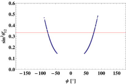
Figure 1: The allowed region on $\psi$–$\sin^{2}\theta_{12}^{\nu}$ plane. The red line corresponds to the TBM.

In this subsection, we show the numerical results in the case of the lightest neutrino mass $m_{3}=0$. In order to reproduce the relevant mass squared differences, $\Delta m_{\rm atm}^{2}$ and $\Delta m_{\rm sol}^{2}$ for the inverted mass hierarchy, $a\simeq 3b$ and $\varphi\simeq\pm\pi$ should be satisfied. Then, the $\psi$ of Eq. (12) is restricted in $45^{\circ}\lesssim|\psi|\lesssim 90^{\circ}$. On the other hand, $\sin\eta$ in Eq. (12) is restricted in $-0.70\lesssim\sin\eta\lesssim-0.38$. In Fig.1, we show the allowed region on $\psi$–$\sin^{2}\theta_{12}^{\nu}$ plane, where $\theta_{12}^{\nu}$ is the mixing angle of the neutrino sector without the charged lepton contribution as seen in Eq.(24). As seen in this figure, our model is possibly deviated from the TBM considerably. Then, the mixing angle and the phase of the charged lepton sector become important to adjust the observed PMNS mixing angles.

Now we can calculate the Dirac phase and the Majorana phases. In Figs. 3 and 3, we show the Dirac phase $\delta_{\text{CP}}$ versus the Majorana phases $\alpha$ and $\beta$, respectively. The both positive and negative signs are allowed for $\alpha$ and $\beta$. The allowed regions of the Majorana phases are $110^{\circ}\lesssim|\alpha|\lesssim 150^{\circ}$ and $145^{\circ}\lesssim|\beta|\lesssim 170^{\circ}$. On the other hand, the Dirac phase is still allowed in the all region as $-\pi\lesssim\delta_{CP}\lesssim\pi$.

Since the difference between the Majorana phases $\alpha$ and $\beta$ contributes to the $0\nu\beta\beta$, we show the Dirac phase versus $(\alpha-\beta)$ in Fig. 5. We obtain $10^{\circ}\lesssim|\alpha-\beta|\lesssim 50^{\circ}$. We also show the allowed region of the Majorana phases on the $\alpha$–$\beta$ plane in Fig. 5. The Majorana phases $\alpha$ and $\beta$ are restricted in the two regions on this plane.

Figure 2: The predicted region on $\alpha$–$\delta_{CP}$ plane.

Figure 3: The predicted region on $\beta$–$\delta_{CP}$ plane.

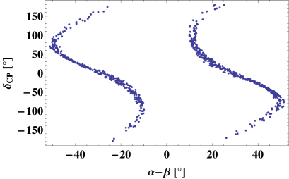
Figure 4: The predicted region on $(\alpha-\beta)$–$\delta_{CP}$ plane.

Figure 5: The predicted region on $\alpha$–$\beta$ plane. The Majorana phases are restricted in the conner on this plane.

Based on the numerical results of the phases, we can estimate the effective neutrino mass for the $0\nu\beta\beta$. The effective neutrino mass is written as

$$m_{ee}\equiv\sum_{i=1}^{3}m_{i}U_{ei}^{2}~{}.$$ (51)

We show the effective neutrino mass of the $0\nu\beta\beta$ versus the difference of the Majorana phases and the Dirac phase for in Figs. 7 and 7, respectively. For the fixed effective neutrino mass for the $0\nu\beta\beta$, there are two fold degeneracy and four fold degeneracy in the Majorana phase $(\alpha-\beta)$ and the Dirac phase $\delta_{CP}$, respectively. Therefore, the degeneracy will be solved if both $\delta_{CP}$ and $m_{ee}$ are observed. At present, we predict $32~{}\text{meV}\lesssim|m_{ee}|\lesssim 49~{}\text{meV}$, which is close to the expected reaches of the coming experiments of the $0\nu\beta\beta$ [131].

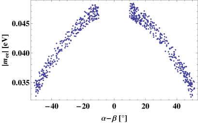
Figure 6: The predicted effective neutrino mass for the $0\nu\beta\beta$ versus $(\alpha-\beta)$.

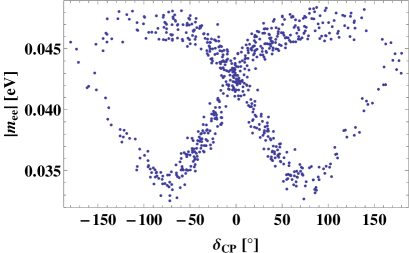
Figure 7: The predicted effective neutrino mass for the $0\nu\beta\beta$ versus $\delta_{CP}$.

Finally, we show the sum of the neutrino masses is predicted as

$$0.0952~{}\text{eV}\lesssim{\displaystyle\sum_{i}}m_{i}\lesssim 0.101~{}\text{eV}.$$ (52)

This total neutrino mass is within the reaches of the future cosmological and astrophysical measurements, such as the CMB spectrum, the galaxy distributions, and the red-shifted 21cm line in the future [132].

3.2 $S_{4}$ flavor model for $m_{3}\not=0$

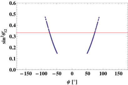
Figure 8: The allowed region on $\psi$–$\sin^{2}\theta_{12}^{\nu}$ plane. The red line corresponds to the TBM.

In this subsection, we show the numerical results in the case of the non-vanishing lightest neutrino mass $m_{3}\not=0$. In order to reproduce the relevant mass squared differences, $\Delta m_{\rm atm}^{2}$ and $\Delta m_{\rm sol}^{2}$ for the inverted mass hierarchy, $a\simeq b$ and $\varphi\simeq\pm\pi$ are satisfied. Then, the $\psi$ of Eq. (36) is restricted in $50^{\circ}\lesssim|\psi|\lesssim 90^{\circ}$ numerically. On the other hand, $\sin\eta$ in Eq. (36) is restricted in $-0.70\lesssim\sin\eta\lesssim-0.54$.

In Fig. 8, we show the allowed region on $\psi$–$\sin^{2}\theta_{12}^{\nu}$ plane, where $\theta_{12}^{\nu}$ is the mixing angle of the neutrino sector without the charged lepton contribution as seen in Eq.(24). This result is very similar to the case of $m_{3}=0$ of Fig. 1 in the previous subsection.

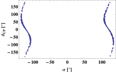
Figure 9: The predicted region on $\alpha$–$\delta_{CP}$ plane.

Figure 10: The predicted region on $\beta$–$\delta_{CP}$ plane.

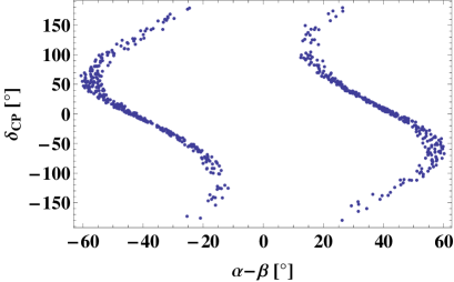
Figure 11: The predicted region on $(\alpha-\beta)$–$\delta_{CP}$ plane.

Figure 12: The predicted region on $\alpha$–$\beta$ plane. The Majorana phases are restricted in the conner of this plane.

At first, in Figs. 10 and 10, we show the Dirac phase $\delta_{\text{CP}}$ versus the Majorana phases $\alpha$ and $\beta$, respectively. The both positive and negative signs are allowed for $\alpha$ and $\beta$. The allowed regions of the Majorana phases are $105^{\circ}\lesssim|\alpha|\lesssim 135^{\circ}$ and $145^{\circ}\lesssim|\beta|\lesssim 170^{\circ}$. The Dirac phase is still allowed in the all region as $-\pi\lesssim\delta_{CP}\lesssim\pi$. We also show the Dirac phase $\delta_{CP}$ versus $(\alpha-\beta)$ in Fig. 12. We obtain $10^{\circ}\lesssim|\alpha-\beta|\lesssim 60^{\circ}$. In Fig. 12, we show the allowed region of the Majorana phases $\alpha$ and $\beta$. The Majorana phases are restricted in the two regions on this plane as well as the case of the previous subsection.

Next, we also show the effective neutrino mass $m_{ee}$ for the $0\nu\beta\beta$ versus the Dirac phase in Fig. 14. For the fixed effective neutrino mass for the $0\nu\beta\beta$, there are four fold degeneracy in the Dirac phase $\delta_{CP}$ as well as the case of the previous subsection. This degeneracy will be solved if both $\delta_{CP}$ and $m_{ee}$ are observed. The predicted magnitude of $m_{ee}$ is $34~{}\text{meV}\lesssim|m_{ee}|\lesssim 59~{}\text{meV}$, which is close to the expected reaches of the coming experiments of the $0\nu\beta\beta$ [131].

Finally, we show the allowed region of neutrino masses $m_{2}$ and $m_{3}$ in Fig. 14. The neutrino mass $m_{2}$ is $58.7~{}\text{meV}\lesssim m_{2}\lesssim 62.2~{}\text{meV}$. The lightest neutrino mass $m_{3}$ is $31.0~{}\text{meV}\lesssim m_{3}\lesssim 35.8~{}\text{meV}$. The sum of the neutrino masses is predicted as

$$0.150~{}\text{eV}\lesssim{\displaystyle\sum_{i}}m_{i}\lesssim 0.160~{}\text{eV}.$$ (53)

This value is also within the reaches of the future cosmological and astrophysical measurements.

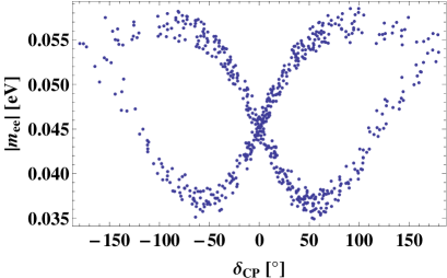
Figure 13: The prediction on $\delta_{CP}$–$|m_{ee}|$ plane. The allowed region of effective neutrino mass for the $0\nu\beta\beta$ is $34~{}\text{meV}\lesssim|m_{ee}|\lesssim 59~{}\text{meV}$.

Figure 14: The allowed region on $m_{3}$–$m_{2}$ plane. The lightest neutrino mass $m_{3}$ is proportional to $m_{2}$.

4 Discussions and Summary

We have presented the minimal $S_{4}$ flavor models of leptons. By using the alignments of the VEV’s of the flavons obtained in subsection 2.3, the models lead to the two different neutrino mass spectra with the inverted mass hierarchy. The neutrino mass matrix is given by two complex parameters in Eqs.(5) and (30). The first case has one vanishing neutrino mass $m_{3}=0$, and the second case has three non-vanishing neutrino masses. The charged leptons are not flavor diagonal. There remains the first and second family mixing, which give the non-vanishing reactor angle $\theta_{13}$. We have moved to the TBM basis of neutrinos in order to clarify the deviation from the TBM.

It is not necessary to go to the TBM basis to calculate the mixing angles, but this is merely a convenient basis to do so. We present alternative basis, the bi-maximal base or the $\mu$-$\tau$ symmetric one, where it is also convenient to study the mass matrices in appendices B and C, respectively.

Inputting the experimental data of two neutrino mass squared differences and the mixing angles $\theta_{12}$, $\theta_{23}$ and $\theta_{13}$, we can predict the Dirac phase and the Majorana phases. Furthermore, we predict the magnitude of the effective neutrino mass of the $0\nu\beta\beta$, which is correlated with the Dirac phases. For the fixed effective neutrino mass for the $0\nu\beta\beta$, there are two fold degeneracy and four fold degeneracy in the Majorana phase difference $(\alpha-\beta)$ and the Dirac phase $\delta_{CP}$, respectively. Therefore, if both $\delta_{CP}$ and $m_{ee}$ are observed, the Majorana phases are determined finally. At present, the predicted magnitudes of $m_{ee}$ are in the regions as $32~{}\text{meV}\lesssim|m_{ee}|\lesssim 49~{}\text{meV}$ and $34~{}\text{meV}\lesssim|m_{ee}|\lesssim 59~{}\text{meV}$ for the cases of $m_{3}=0$ and $m_{3}\not=0$, respectively. These values are close to the expected reaches of the coming experiments of the $0\nu\beta\beta$.

The sum of three neutrino masses is also predicted in both models as $0.0952~{}\text{eV}\lesssim\sum m_{i}\lesssim 0.101~{}\text{eV}$ and $0.150~{}\text{eV}\lesssim\sum m_{i}\lesssim 0.160~{}\text{eV}$, respectively. Those total masses are also within the reaches of the future cosmological and astrophysical measurements.

Acknowledgement

This work is supported by JSPS Grant-in-Aid for Scientific Research, 15K05045.

Appendix

Appendix A Multiplication rules of the $S_{4}$ group

We show the multiplication rules of $S_{4}$:

$$\begin{pmatrix}a_{1}\\ a_{2}\end{pmatrix}_{\bf 2}\otimes\begin{pmatrix}b_{1}\\ b_{2}\end{pmatrix}_{\bf 2} =(a_{1}b_{1}+a_{2}b_{2})_{{\bf 1}}\oplus(-a_{1}b_{2}+a_{2}b_{1})_{{\bf 1}^{\prime}}\oplus\begin{pmatrix}a_{1}b_{2}+a_{2}b_{1}\\ a_{1}b_{1}-a_{2}b_{2}\end{pmatrix}_{{\bf 2}\ ,}$$

$$\begin{pmatrix}a_{1}\\ a_{2}\end{pmatrix}_{\bf 2}\otimes\begin{pmatrix}b_{1}\\ b_{2}\\ b_{3}\end{pmatrix}_{{\bf 3}} =\begin{pmatrix}a_{2}b_{1}\\ -\frac{1}{2}(\sqrt{3}a_{1}b_{2}+a_{2}b_{2})\\ \frac{1}{2}(\sqrt{3}a_{1}b_{3}-a_{2}b_{3})\end{pmatrix}_{{\bf 3}}\oplus\begin{pmatrix}a_{1}b_{1}\\ \frac{1}{2}(\sqrt{3}a_{2}b_{2}-a_{1}b_{2})\\ -\frac{1}{2}(\sqrt{3}a_{2}b_{3}+a_{1}b_{3})\end{pmatrix}_{{\bf 3}^{\prime}\ ,}$$

$$\begin{pmatrix}a_{1}\\ a_{2}\end{pmatrix}_{\bf 2}\otimes\begin{pmatrix}b_{1}\\ b_{2}\\ b_{3}\end{pmatrix}_{{\bf 3}^{\prime}} =\begin{pmatrix}a_{1}b_{1}\\ \frac{1}{2}(\sqrt{3}a_{2}b_{2}-a_{1}b_{2})\\ -\frac{1}{2}(\sqrt{3}a_{2}b_{3}+a_{1}b_{3})\end{pmatrix}_{{\bf 3}}\oplus\begin{pmatrix}a_{2}b_{1}\\ -\frac{1}{2}(\sqrt{3}a_{1}b_{2}+a_{2}b_{2})\\ \frac{1}{2}(\sqrt{3}a_{1}b_{3}-a_{2}b_{3})\end{pmatrix}_{{\bf 3}^{\prime}\ ,}$$

$$\begin{pmatrix}a_{1}\\ a_{2}\\ a_{3}\end{pmatrix}_{{\bf 3}}\otimes\begin{pmatrix}b_{1}\\ b_{2}\\ b_{3}\end{pmatrix}_{{\bf 3}} =(a_{1}b_{1}+a_{2}b_{2}+a_{3}b_{3})_{{\bf 1}}\oplus\begin{pmatrix}\frac{1}{\sqrt{2}}(a_{2}b_{2}-a_{3}b_{3})\\ \frac{1}{\sqrt{6}}(-2a_{1}b_{1}+a_{2}b_{2}+a_{3}b_{3})\end{pmatrix}_{\bf 2}$$

$$\ \oplus\begin{pmatrix}a_{2}b_{3}+a_{3}b_{2}\\ a_{1}b_{3}+a_{3}b_{1}\\ a_{1}b_{2}+a_{2}b_{1}\end{pmatrix}_{{\bf 3}}\oplus\begin{pmatrix}a_{3}b_{2}-a_{2}b_{3}\\ a_{1}b_{3}-a_{3}b_{1}\\ a_{2}b_{1}-a_{1}b_{2}\end{pmatrix}_{{\bf 3}^{\prime}\ ,}$$

$$\begin{pmatrix}a_{1}\\ a_{2}\\ a_{3}\end{pmatrix}_{{\bf 3}^{\prime}}\otimes\begin{pmatrix}b_{1}\\ b_{2}\\ b_{3}\end{pmatrix}_{{\bf 3}^{\prime}} =(a_{1}b_{1}+a_{2}b_{2}+a_{3}b_{3})_{{\bf 1}}\oplus\begin{pmatrix}\frac{1}{\sqrt{2}}(a_{2}b_{2}-a_{3}b_{3})\\ \frac{1}{\sqrt{6}}(-2a_{1}b_{1}+a_{2}b_{2}+a_{3}b_{3})\end{pmatrix}_{\bf 2}$$

$$\ \oplus\begin{pmatrix}a_{2}b_{3}+a_{3}b_{2}\\ a_{1}b_{3}+a_{3}b_{1}\\ a_{1}b_{2}+a_{2}b_{1}\end{pmatrix}_{{\bf 3}}\oplus\begin{pmatrix}a_{3}b_{2}-a_{2}b_{3}\\ a_{1}b_{3}-a_{3}b_{1}\\ a_{2}b_{1}-a_{1}b_{2}\end{pmatrix}_{{\bf 3}^{\prime}\ ,}$$

$$\begin{pmatrix}a_{1}\\ a_{2}\\ a_{3}\end{pmatrix}_{{\bf 3}}\otimes\begin{pmatrix}b_{1}\\ b_{2}\\ b_{3}\end{pmatrix}_{{\bf 3}^{\prime}} =(a_{1}b_{1}+a_{2}b_{2}+a_{3}b_{3})_{{\bf 1}^{\prime}}\oplus\begin{pmatrix}\frac{1}{\sqrt{6}}(2a_{1}b_{1}-a_{2}b_{2}-a_{3}b_{3})\\ \frac{1}{\sqrt{2}}(a_{2}b_{2}-a_{3}b_{3})\end{pmatrix}_{\bf 2}$$

$$\ \oplus\begin{pmatrix}a_{3}b_{2}-a_{2}b_{3}\\ a_{1}b_{3}-a_{3}b_{1}\\ a_{2}b_{1}-a_{1}b_{2}\end{pmatrix}_{{\bf 3}}\oplus\begin{pmatrix}a_{2}b_{3}+a_{3}b_{2}\\ a_{1}b_{3}+a_{3}b_{1}\\ a_{1}b_{2}+a_{2}b_{1}\end{pmatrix}_{{\bf 3}^{\prime}\ .}$$ (54)

More details are shown in the review [41, 42].

Appendix B Neutrino mass matrix in the bimaximal base

B.1 $m_{3}=0$ case

The left-handed Majorana neutrino mass matrix $M_{\nu}$ is

$$M_{\nu}=\begin{pmatrix}a+b&b&b\\ b&b&b\\ b&b&b\end{pmatrix}.$$ (55)

After rotating $M_{\nu}$ with the bimaximal mixing matrix $V_{\text{BM}}$ as

$$V_{\text{BM}}=\begin{pmatrix}\frac{1}{\sqrt{2}}&\frac{1}{\sqrt{2}}&0\\ -\frac{1}{2}&\frac{1}{2}&-\frac{1}{\sqrt{2}}\\ -\frac{1}{2}&\frac{1}{2}&\frac{1}{\sqrt{2}}\end{pmatrix},$$ (56)

the left-handed Majorana neutrino mass matrix is rewritten as

$$M_{\nu}=V_{\text{BM}}\begin{pmatrix}\frac{1}{2}\left(a+(3-2\sqrt{2})b\right)&\frac{1}{2}(a-b)&0\\ \frac{1}{2}(a-b)&\frac{1}{2}\left(a+(3+2\sqrt{2})b\right)&0\\ 0&0&0\end{pmatrix}V_{\text{BM}}^{T}~{}.$$ (57)

B.2 $m_{3}\not=0$ case

The left-handed Majorana neutrino mass matrix $M_{\nu}$ is

$$M_{\nu}=\begin{pmatrix}b&b&b\\ b&2a+b&a+b\\ b&a+b&2a+b\end{pmatrix}.$$ (58)

After rotating $M_{\nu}$ with the bimaximal mixing matrix $V_{\text{BM}}$, the left-handed Majorana neutrino mass matrix is rewritten as

$$M_{\nu}=V_{\text{BM}}\begin{pmatrix}\frac{1}{2}\left(3a+(3-2\sqrt{2})b\right)&-\frac{1}{2}(3a+b)&0\\ -\frac{1}{2}(3a+b)&\frac{1}{2}\left(3a+(3+2\sqrt{2})b\right)&0\\ 0&0&a\end{pmatrix}V_{\text{BM}}^{T}~{}.$$ (59)

Appendix C Neutrino mass matrix in the $\mu$-$\tau$ maximal base

C.1 $m_{3}=0$ case

The left-handed Majorana neutrino mass matrix $M_{\nu}$ is

$$M_{\nu}=\begin{pmatrix}a+b&b&b\\ b&b&b\\ b&b&b\end{pmatrix}.$$ (60)

After rotating $M_{\nu}$ with the $\mu$-$\tau$ maximal mixing matrix $V_{23}$ as

$$V_{23}=\begin{pmatrix}1&0&0\\ 0&\frac{1}{\sqrt{2}}&-\frac{1}{\sqrt{2}}\\ 0&\frac{1}{\sqrt{2}}&\frac{1}{\sqrt{2}}\end{pmatrix},$$ (61)

the left-handed Majorana neutrino mass matrix is rewritten as

$$M_{\nu}=V_{23}\begin{pmatrix}a+b&\sqrt{2}b&0\\ \sqrt{2}b&2b&0\\ 0&0&0\end{pmatrix}V_{23}^{T}~{}.$$ (62)

C.2 $m_{3}\not=0$ case

The left-handed Majorana neutrino mass matrix $M_{\nu}$ is

$$M_{\nu}=\begin{pmatrix}b&b&b\\ b&2a+b&a+b\\ b&a+b&2a+b\end{pmatrix}.$$ (63)

After rotating $M_{\nu}$ with the $\mu$-$\tau$ maximal mixing matrix $V_{23}$, the left-handed Majorana neutrino mass matrix is rewritten as

$$M_{\nu}=V_{23}\begin{pmatrix}b&\sqrt{2}b&0\\ \sqrt{2}b&3a+2b&0\\ 0&0&a\end{pmatrix}V_{23}^{T}~{}.$$ (64)

References

- [1] S. M. Bilenky, J. Hosek and S. T. Petcov, Phys. Lett. B 94 (1980) 495.
- [2] J. Schechter and J. W. F. Valle, Phys. Rev. D 22 (1980) 2227.
- [3] M. Doi, T. Kotani, H. Nishiura, K. Okuda and E. Takasugi, Phys. Lett. B 102 (1981) 323.
- [4] K. Abe et al. [T2K Collaboration], Phys. Rev. Lett. 112 (2014) 061802 [arXiv:1311.4750 [hep-ex]].
- [5] F. P. An et al. [DAYA-BAY Collaboration], Phys. Rev. Lett. 108 (2012) 171803 [arXiv:1203.1669 [hep-ex]].
- [6] J. K. Ahn et al. [RENO Collaboration], Phys. Rev. Lett. 108 (2012) 191802 [arXiv:1204.0626 [hep-ex]].
- [7] P. Adamson et al. [MINOS Collaboration], Phys. Rev. Lett. 110 (2013) 25, 251801 [arXiv:1304.6335 [hep-ex]].
- [8] Y. Abe et al. [Double Chooz Collaboration], Phys. Lett. B 735 (2014) 51 [arXiv:1401.5981 [hep-ex]].
- [9] S. K. Kang, C. S. Kim and J. D. Kim, Phys. Rev. D 62 (2000) 073011 [hep-ph/0004020].
- [10] M. Fukugita and M. Tanimoto, Phys. Lett. B 515 (2001) 30 [hep-ph/0107082].
- [11] C. Giunti and M. Tanimoto, Phys. Rev. D 66 (2002) 113006 [hep-ph/0209169].
- [12] Z. -z. Xing, Phys. Lett. B 533 (2002) 85 [hep-ph/0204049].
- [13] B. Adhikary and A. Ghosal, Phys. Rev. D 75 (2007) 073020 [hep-ph/0609193].
- [14] B. Adhikary and A. Ghosal, Phys. Rev. D 78 (2008) 073007 [arXiv:0803.3582 [hep-ph]].
- [15] G. C. Branco, R. G. Felipe and F. R. Joaquim, Rev. Mod. Phys. 84 (2012) 515 [arXiv:1111.5332 [hep-ph]].
- [16] G. C. Branco, R. Gonzalez Felipe, F. R. Joaquim and H. Serodio, Phys. Rev. D 86 (2012) 076008 [arXiv:1203.2646 [hep-ph]].
- [17] Y. H. Ahn and S. K. Kang, Phys. Rev. D 86 (2012) 093003 [arXiv:1203.4185 [hep-ph]].
- [18] H. Ishimori, S. Khalil and E. Ma, Phys. Rev. D 86 (2012) 013008 [arXiv:1204.2705 [hep-ph]].
- [19] H. Ishimori and E. Ma, Phys. Rev. D 86 (2012) 045030 [arXiv:1205.0075 [hep-ph]].
- [20] W. Rodejohann and H. Zhang, Phys. Rev. D 86 (2012) 093008 [arXiv:1207.1225 [hep-ph]].
- [21] D. Marzocca, S. T. Petcov, A. Romanino and M. C. Sevilla, JHEP 1305 (2013) 073 [arXiv:1302.0423 [hep-ph]].
- [22] P. Ballett, S. F. King, C. Luhn, S. Pascoli and M. A. Schmidt, Phys. Rev. D 89 (2014) 1, 016016 [arXiv:1308.4314 [hep-ph]].
- [23] P. Ballett, S. F. King, C. Luhn, S. Pascoli and M. A. Schmidt, JHEP 1412 (2014) 122 [arXiv:1410.7573 [hep-ph]].
- [24] Z. z. Xing and S. Zhou, Phys. Lett. B 737 (2014) 196 [arXiv:1404.7021 [hep-ph]].
- [25] G. C. Branco, M. N. Rebelo, J. I. Silva-Marcos and D. Wegman, Phys. Rev. D 91 (2015) 013001 [arXiv:1405.5120 [hep-ph]].
- [26] S. T. Petcov, Nucl. Phys. B 892 (2015) 400 [arXiv:1405.6006 [hep-ph]].
- [27] S. K. Kang and C. S. Kim, Phys. Rev. D 90 (2014) 7, 077301 [arXiv:1406.5014 [hep-ph]].
- [28] Y. Shimizu, M. Tanimoto and K. Yamamoto, Mod. Phys. Lett. A, 30 (2015) 1550002 [arXiv:1405.1521 [hep-ph]].
- [29] I. Girardi, S. T. Petcov and A. V. Titov, Nucl. Phys. B 894 (2015) 733 [arXiv:1410.8056 [hep-ph]].
- [30] I. Girardi, S. T. Petcov and A. V. Titov, Int. J. Mod. Phys. A 30 (2015) 13, 1530035 [arXiv:1504.02402 [hep-ph]].
- [31] I. Girardi, S. T. Petcov and A. V. Titov, arXiv:1504.00658 [hep-ph].
- [32] S. K. Kang and M. Tanimoto, Phys. Rev. D 91 (2015) 7, 073010 [arXiv:1501.07428 [hep-ph]].
- [33] P. F. Harrison, D. H. Perkins, W. G. Scott, Phys. Lett. B 530 (2002) 167 [hep-ph/0202074].
- [34] P. F. Harrison, W. G. Scott, Phys. Lett. B 535 (2002) 163-169 [hep-ph/0203209].
- [35] E. Ma and G. Rajasekaran, Phys. Rev. D 64 (2001) 113012 [hep-ph/0106291].
- [36] K. S. Babu, E. Ma and J. W. F. Valle, Phys. Lett. B 552 (2003) 207 [hep-ph/0206292].
- [37] G. Altarelli and F. Feruglio, Nucl. Phys. B 720 (2005) 64 [hep-ph/0504165].
- [38] G. Altarelli and F. Feruglio, Nucl. Phys. B 741 (2006) 215 [hep-ph/0512103].
- [39] I. de Medeiros Varzielas, S. F. King and G. G. Ross, Phys. Lett. B 644 (2007) 153 [hep-ph/0512313].
- [40] G. Altarelli and F. Feruglio, Rev. Mod. Phys. 82 (2010) 2701 [arXiv:1002.0211 [hep-ph]].
- [41] H. Ishimori, T. Kobayashi, H. Ohki, Y. Shimizu, H. Okada and M. Tanimoto, Prog. Theor. Phys. Suppl. 183 (2010) 1 [arXiv:1003.3552 [hep-th]].
- [42] H. Ishimori, T. Kobayashi, H. Ohki, H. Okada, Y. Shimizu and M. Tanimoto, Lect. Notes Phys. 858 (2012) 1.
- [43] S. F. King, A. Merle, S. Morisi, Y. Shimizu and M. Tanimoto, New J. Phys. 16 (2014) 045018 [arXiv:1402.4271 [hep-ph]].
- [44] R. N. Mohapatra, S. Nasri and H. -B. Yu, Phys. Lett. B 639 (2006) 318 [hep-ph/0605020].
- [45] I. de Medeiros Varzielas, S. F. King and G. G. Ross, Phys. Lett. B 648 (2007) 201 [hep-ph/0607045].
- [46] P. D. Carr and P. H. Frampton, hep-ph/0701034.
- [47] F. Feruglio, C. Hagedorn, Y. Lin and L. Merlo, Nucl. Phys. B 775 (2007) 120 [Erratum-ibid. 836 (2010) 127] [hep-ph/0702194].
- [48] C. S. Lam, Phys. Rev. Lett. 101 (2008) 121602 [arXiv:0804.2622 [hep-ph]].
- [49] F. Bazzocchi and S. Morisi, Phys. Rev. D 80 (2009) 096005 [arXiv:0811.0345 [hep-ph]].
- [50] W. Grimus and L. Lavoura, JHEP 0809 (2008) 106 [arXiv:0809.0226 [hep-ph]].
- [51] W. Grimus and L. Lavoura, JHEP 0904 (2009) 013 [arXiv:0811.4766 [hep-ph]].
- [52] H. Ishimori, T. Kobayashi, H. Okada, Y. Shimizu and M. Tanimoto, JHEP 0904 (2009) 011 [arXiv:0811.4683 [hep-ph]].
- [53] F. Bazzocchi, L. Merlo and S. Morisi, Nucl. Phys. B 816 (2009) 204 [arXiv:0901.2086 [hep-ph]].
- [54] F. Bazzocchi, L. Merlo and S. Morisi, Phys. Rev. D 80 (2009) 053003 [arXiv:0902.2849 [hep-ph]].
- [55] G. Altarelli, F. Feruglio and L. Merlo, JHEP 0905 (2009) 020 [arXiv:0903.1940 [hep-ph]].
- [56] Z. -z. Xing and S. Zhou, Phys. Lett. B 653 (2007) 278 [hep-ph/0607302].
- [57] S. F. King, Phys. Lett. B 659 (2008) 244 [arXiv:0710.0530 [hep-ph]].
- [58] M. Honda and M. Tanimoto, Prog. Theor. Phys. 119 (2008) 583 [arXiv:0801.0181 [hep-ph]].
- [59] M. Hirsch, S. Morisi and J. W. F. Valle, Phys. Rev. D 79 (2009) 016001 [arXiv:0810.0121 [hep-ph]].
- [60] S. Morisi, Phys. Rev. D 79 (2009) 033008 [arXiv:0901.1080 [hep-ph]].
- [61] A. Hayakawa, H. Ishimori, Y. Shimizu and M. Tanimoto, Phys. Lett. B 680 (2009) 334 [arXiv:0904.3820 [hep-ph]].
- [62] J. Barry and W. Rodejohann, Phys. Rev. D 81 (2010) 093002 [Phys. Rev. D 81 (2010) 119901] [arXiv:1003.2385 [hep-ph]].
- [63] C. H. Albright, A. Dueck and W. Rodejohann, Eur. Phys. J. C 70 (2010) 1099 [arXiv:1004.2798 [hep-ph]].
- [64] H. Ishimori, Y. Shimizu, M. Tanimoto and A. Watanabe, Phys. Rev. D 83 (2011) 033004 [arXiv:1010.3805 [hep-ph]].
- [65] I. de Medeiros Varzielas and L. Merlo, JHEP 1102 (2011) 062 [arXiv:1011.6662 [hep-ph]].
- [66] S. F. King and C. Luhn, JHEP 1109 (2011) 042 [arXiv:1107.5332 [hep-ph]].
- [67] S. F. King and C. Luhn, JHEP 1203 (2012) 036 [arXiv:1112.1959 [hep-ph]].
- [68] Y. Shimizu, M. Tanimoto and A. Watanabe, Prog. Theor. Phys. 126 (2011) 81 [arXiv:1105.2929 [hep-ph]].
- [69] E. Ma and D. Wegman, Phys. Rev. Lett. 107 (2011) 061803 [arXiv:1106.4269 [hep-ph]].
- [70] H. Ishimori and T. Kobayashi, JHEP 1110 (2011) 082 [arXiv:1106.3604 [hep-ph]].
- [71] S. Antusch and V. Maurer, Phys. Rev. D 84 (2011) 117301 [arXiv:1107.3728 [hep-ph]].
- [72] P. S. Bhupal Dev, R. N. Mohapatra and M. Severson, Phys. Rev. D 84 (2011) 053005 [arXiv:1107.2378 [hep-ph]].
- [73] P. S. Bhupal Dev, B. Dutta, R. N. Mohapatra and M. Severson, Phys. Rev. D 86 (2012) 035002 [arXiv:1202.4012 [hep-ph]].
- [74] F. Bazzocchi and L. Merlo, Fortsch. Phys. 61 (2013) 571 [arXiv:1205.5135 [hep-ph]].
- [75] J. A. Acosta, A. Aranda, M. A. Buen-Abad and A. D. Rojas, Phys. Lett. B 718 (2013) 1413 [arXiv:1207.6093 [hep-ph]].
- [76] C. Hagedorn, S. F. King and C. Luhn, Phys. Lett. B 717 (2012) 207 [arXiv:1205.3114].
- [77] G. Altarelli, F. Feruglio, L. Merlo and E. Stamou, JHEP 1208 (2012) 021 [arXiv:1205.4670 [hep-ph]].
- [78] G. Altarelli, F. Feruglio and L. Merlo, Fortsch. Phys. 61 (2013) 507 [arXiv:1205.5133 [hep-ph]].
- [79] S. F. King, Phys. Lett. B 718 (2012) 136 [arXiv:1205.0506 [hep-ph]].
- [80] S. F. King, T. Neder and A. J. Stuart, Phys. Lett. B 726 (2013) 312 [arXiv:1305.3200 [hep-ph]].
- [81] Y. Shimizu, R. Takahashi and M. Tanimoto, PTEP 2013 (2013) 6, 063B02 [arXiv:1212.5913 [hep-ph]].
- [82] S. F. King, JHEP 1307 (2013) 137 [arXiv:1304.6264 [hep-ph]].
- [83] S. F. King, Phys. Lett. B 724 (2013) 92 [arXiv:1305.4846 [hep-ph]].
- [84] W. Grimus and L. Lavoura, Phys. Lett. B 579 (2004) 113 [hep-ph/0305309].
- [85] M. C. Chen and K. T. Mahanthappa, Phys. Lett. B 681 (2009) 444 [arXiv:0904.1721 [hep-ph]].
- [86] F. Feruglio, C. Hagedorn and R. Ziegler, Eur. Phys. J. C 74 (2014) 2753 [arXiv:1303.7178 [hep-ph]].
- [87] G. J. Ding, S. F. King and A. J. Stuart, JHEP 1312 (2013) 006 [arXiv:1307.4212 [hep-ph]].
- [88] P. M. Ferreira, W. Grimus, L. Lavoura and P. O. Ludl, JHEP 1209 (2012) 128 [arXiv:1206.7072 [hep-ph]].
- [89] I. de Medeiros Varzielas and D. Emmanuel-Costa, Phys. Rev. D 84 (2011) 117901 [arXiv:1106.5477 [hep-ph]].
- [90] S. Morisi, K. M. Patel and E. Peinado, Phys. Rev. D 84 (2011) 053002 [arXiv:1107.0696 [hep-ph]].
- [91] S. Gupta, A. S. Joshipura and K. M. Patel, Phys. Rev. D 85 (2012) 031903 [arXiv:1112.6113 [hep-ph]].
- [92] I. de Medeiros Varzielas, JHEP 1208 (2012) 055 [arXiv:1205.3780 [hep-ph]].
- [93] I. de Medeiros Varzielas, D. Emmanuel-Costa and P. Leser, Phys. Lett. B 716 (2012) 193 [arXiv:1204.3633 [hep-ph]].
- [94] M. Holthausen, M. Lindner and M. A. Schmidt, JHEP 1304 (2013) 122 [arXiv:1211.6953 [hep-ph]].
- [95] M. C. Chen, M. Fallbacher, K. T. Mahanthappa, M. Ratz and A. Trautner, Nucl. Phys. B 883 (2014) 267 [arXiv:1402.0507 [hep-ph]].
- [96] R. N. Mohapatra and C. C. Nishi, Phys. Rev. D 86 (2012) 073007 [arXiv:1208.2875 [hep-ph]].
- [97] E. Ma, Phys. Lett. B 723 (2013) 161 [arXiv:1304.1603 [hep-ph]].
- [98] I. Girardi, A. Meroni, S. T. Petcov and M. Spinrath, JHEP 1402 (2014) 050 [arXiv:1312.1966 [hep-ph]].
- [99] G. J. Ding, S. F. King, C. Luhn and A. J. Stuart, JHEP 1305 (2013) 084 [arXiv:1303.6180 [hep-ph]].
- [100] A. Meroni, S. T. Petcov and M. Spinrath, Phys. Rev. D 86 (2012) 113003 [arXiv:1205.5241 [hep-ph]].
- [101] C. C. Li and G. J. Ding, Nucl. Phys. B 881 (2014) 206 [arXiv:1312.4401 [hep-ph]].
- [102] C. Luhn, Nucl. Phys. B 875 (2013) 80 [arXiv:1306.2358 [hep-ph]].
- [103] G. J. Ding and Y. L. Zhou, Chin. Phys. C 39 (2015) 2, 021001 [arXiv:1312.5222 [hep-ph]].
- [104] P. Chen, C. C. Li and G. J. Ding, Phys. Rev. D 91 (2015) 3, 033003 [arXiv:1412.8352 [hep-ph]].
- [105] C. C. Li and G. J. Ding, JHEP 1505 (2015) 100 [arXiv:1503.03711 [hep-ph]].
- [106] F. Bazzocchi, M. Frigerio and S. Morisi, Phys. Rev. D 78 (2008) 116018 [arXiv:0809.3573 [hep-ph]].
- [107] H. Ishimori, Y. Shimizu and M. Tanimoto, Prog. Theor. Phys. 121 (2009) 769 [arXiv:0812.5031 [hep-ph]].
- [108] H. Ishimori, K. Saga, Y. Shimizu and M. Tanimoto, Phys. Rev. D 81 (2010) 115009 [arXiv:1004.5004 [hep-ph]].
- [109] R. de Adelhart Toorop, F. Bazzocchi and L. Merlo, JHEP 1008 (2010) 001 [arXiv:1003.4502 [hep-ph]].
- [110] I. K. Cooper, S. F. King and C. Luhn, Phys. Lett. B 690 (2010) 396 [arXiv:1004.3243 [hep-ph]].
- [111] I. K. Cooper, S. F. King and C. Luhn, JHEP 1206 (2012) 130 [arXiv:1203.1324 [hep-ph]].
- [112] S. F. King and C. Luhn, Nucl. Phys. B 832 (2010) 414 [arXiv:0912.1344 [hep-ph]].
- [113] A. S. Joshipura, B. P. Kodrani and K. M. Patel, Phys. Rev. D 79 (2009) 115017 [arXiv:0903.2161 [hep-ph]].
- [114] K. M. Patel, Phys. Lett. B 695 (2011) 225 [arXiv:1008.5061 [hep-ph]].
- [115] A. S. Joshipura and K. M. Patel, Phys. Rev. D 83 (2011) 095002 [arXiv:1102.5148 [hep-ph]].
- [116] C. Hagedorn, S. F. King and C. Luhn, JHEP 1006 (2010) 048 [arXiv:1003.4249 [hep-ph]].
- [117] S. F. King, C. Luhn and A. J. Stuart, Nucl. Phys. B 867 (2013) 203 [arXiv:1207.5741 [hep-ph]].
- [118] S. Antusch, C. Gross, V. Maurer and C. Sluka, Nucl. Phys. B 877 (2013) 772 [arXiv:1305.6612 [hep-ph]].
- [119] S. F. King, JHEP 1408 (2014) 130 [arXiv:1406.7005 [hep-ph]].
- [120] M. Tanimoto and K. Yamamoto, JHEP 1504 (2015) 037 [arXiv:1501.07717 [hep-ph]].
- [121] C. Y. Yao and G. J. Ding, arXiv:1505.03798 [hep-ph].
- [122] K. Harigaya, M. Ibe and T. T. Yanagida, Phys. Rev. D 86 (2012) 013002 [arXiv:1205.2198 [hep-ph]].
- [123] C. D. Froggatt and H. B. Nielsen, Nucl. Phys. B 147 (1979) 277.
- [124] Z. Maki, M. Nakagawa and S. Sakata, Prog. Theor. Phys. 28 (1962) 870.
- [125] B. Pontecorvo, Sov. Phys. JETP 26 (1968) 984 [Zh. Eksp. Teor. Fiz. 53 (1967) 1717].
- [126] M. C. Gonzalez-Garcia, M. Maltoni and T. Schwetz, JHEP 1411 (2014) 052 [arXiv:1409.5439 [hep-ph]].
- [127] D. V. Forero, M. Tortola and J. W. F. Valle, Phys. Rev. D 86 (2012) 073012 [arXiv:1205.4018 [hep-ph]].
- [128] G. L. Fogli, E. Lisi, A. Marrone, D. Montanino, A. Palazzo and A. M. Rotunno, Phys. Rev. D 86 (2012) 013012 [arXiv:1205.5254 [hep-ph]].
- [129] K.A. Olive et al. (Particle Data Group), Chin. Phys. C, 38, 090001 (2014).
- [130] C. Jarlskog, Phys. Rev. Lett. 55 (1985) 1039.
- [131] J. J. Gomez-Cadenas and J. Martin-Albo, PoS GSSI 14 (2015) 004 [arXiv:1502.00581 [hep-ex]].
- [132] K. N. Abazajian et al. [Topical Conveners: K.N. Abazajian, J.E. Carlstrom, A.T. Lee Collaboration], Astropart. Phys. 63 (2015) 66 [arXiv:1309.5383 [astro-ph.CO]].