Multi-scaling of wholesale electricity prices

Abstract

We empirically analyze the most volatile component of the electricity price time series from two North-American wholesale electricity markets. We show that these time series exhibit fluctuations which are not described by a Brownian Motion, as they show multi-scaling, high Hurst exponents and sharp price movements. We use the generalized Hurst exponent (GHE, $H(q)$) to show that although these time-series have strong cyclical components, the fluctuations exhibit persistent behaviour, i.e., $H(q)>0.5$. We investigate the effectiveness of the GHE as a predictive tool in a simple linear forecasting model, and study the forecast error as a function of $H(q)$, with $q=1$ and $q=2$. Our results suggest that the GHE can be used as prediction tool for these time series when the Hurst exponent is dynamically evaluated on rolling time windows of size $\approx 50-100$ hours. These results are also compared to the case in which the cyclical components have been subtracted from the time series, showing the importance of cyclicality in the prediction power of the Hurst exponent.

1 Introduction

Organized wholesale electricity markets are increasingly replacing vertically integrated systems around the world. These markets attempt to balance the objectives of short term stability and performance with economic competitiveness, efficiency, and long term planning (Hogan (2008), Liu (2009), Loskow (2008), Kwon (2012)). Their structure is designed to take into account the unique properties of electricity among commodities: (i) it currently cannot be economically stored, so supply and demand must be continually balanced, (ii) injections into the transmission network flow according to Kirchhoff’s laws, not from point to point, (iii) the transmission network has finite capacity and many operating constraints which limit the size of injections and withdrawals at specific locations, and (iv) the amount of power demanded is typically insensitive to price over short time periods.

In particular, these properties can lead to situations in which the network becomes segmented into effectively separate regions, meaning that some producers cannot competitively sell energy at certain locations. This segmentation is usually called transmission congestion, and can lead to large inefficiencies and costs to consumers. The standard approach to dealing with the above is to use a spatial and temporal pricing mechanism that explicitly accounts for the physical and operating constraints on the transmission network and generation units (Bohn et al (1984)). In this approach, prices at various locations in the transmission network, which are called Locational Marginal Prices (LMPs), are determined with the objective of maximizing social welfare while taking into account all physical and operating constraints, and compensating production and transmission providers for the marginal costs of their services.

These prices exhibit a very rich structure: they are high frequency, non-stationary, very seasonal, very volatile at times of peak demand and supply shortages, and fat tailed. From many points of view, such as financial risk management, market efficiency, mitigating market power, as well as short and long term planning, it is therefore important to understand the structure and predictability of these prices (Aggarwal et al. (2009), Moest et al. (2010), Benth et al. (2012), Bottazzi et al. (2012), Wang et al (2013), Weron (2006)).

In this paper we show that the fluctuations in the most volatile component of LMPs exhibits multi-scaling behaviour and high generalized Hurst exponent values. In addition, we study the forecast error of simple linear forecasting models, and how this is related to the generalized Hurst exponent.

In Section 2 we discuss the structure of the available data and its properties. In Section 3 we study the seasonality properties of the prices and the multi-scaling behaviour by using the generalized Hurst exponent approach. In Section 4 we connect the properties of the generalized Hurst exponent to the forecast error of a linear predictive model. We conclude in Section 5.

2 Properties of the data

The electricity markets in the United States have adopted what is known as a multi-settlement structure. Market participants freely make bids and offers for electricity at different locations in the transmission network which are fed into a centrally organized dispatch and scheduling system administered by an independent authority, often called an independent system operator (ISO). This bidding and dispatch is managed in a set of successive runs. The first run, performed a day in advance of an operating day, is called the Day-Ahead (DA) market. Using the DA bids, the ISO establishes a generation and load schedule and DA LMPs for each hour of the operating day, at each location (often called node) of the network. The DA market exists to help participants and the ISO plan ahead, increase market liquidity, and mitigate market power (Loskow (2008)). Then, as each hour of the operating day approaches, a Real-Time (RT) energy market is administered based on revised generation offers and load forecast. This process results in new hourly RT LMPs at each node. RT LMPs are much more volatile than DA LMP’s due to changes in fuel costs, unanticipated demand that must be met in real time by existing capacity, as well as planned and unplanned generation and transmission outages.

In more technical terms, the LMP at some node is the marginal cost (expressed in $/MWh) of supplying, at the lowest cost, the next increment of demand at that node, while taking into account supply and demand and the physical and operational constraints of the transmission network. For each node $n$ the DA or RT LMP at time $t$ can be split into three components (Liu (2009)):

$$LMP(n,t)=MEC(t)+MLC(n,t)+MCC(n,t),$$ (1)

where MEC is the Marginal Electricity Component, MLC is the Marginal Loss Component, and MCC stands for Marginal Congestion Component. The $MEC(t)$ component is the price of electricity at any given node if there is no congestion or loss to that node. $MLC$ is the cost of transmission losses to a node, and is generally small in comparison with $MEC$. The $MCC$ component is of particular interest to us: it is related to the congestion occurring in the transmission network and is the most volatile time series in RT and DA, as can be observed in Fig. 1 for a particular node in the MISO market.

For our study we focus on the DA MCC component of price from two markets: the Midwest Independent System Operator (MISO) and Pennsylvania-New Jersey-Maryland Interconnection (PJM), for a period of time of 1632 hours, starting January 1, 2014 and ending March 9, 2014. There are 1287 nodes for PJM and 2568 nodes in MISO.

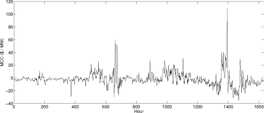
Figure 1: An example of the RT MCC component time series in MISO in the time period of 1632 hours starting on January 1, 2014. The price is the cost per Megawatt-hour of electricity at a particular node. We observe that the congestion component can be both positive and negative and that the price varies over many orders of magnitude.

3 Seasonality and multi-scaling

Given the fact that LMPs are strongly influenced by the local and regional climates and supply and demand patterns, one could ask whether there are any cyclic patterns in LMPs, and if this influences the predictability of the time series (Brown (2012)).

For this purpose, we study the discrete Fourier transform (computed with a Fast Fourier Transform (FFT) algorithm) of the time series of prices $S_{i}(t)$ at each node $i$, from the PJM and MISO markets. In Fig. 2 we plot the power spectrum of each time series, defined as $p_{i}(k)=|\tilde{S}_{i}(k)|^{2}$, with $\tilde{S}_{i}(k)=FFT(S_{i}(t))$, evaluated over the whole time range and averaged over all nodes in the market. The value in each bin $k$ is given by $\langle p(k)\rangle=\frac{1}{N}\sum_{i=1}^{N}p_{i}(k)$, where $N$ is the number of nodes in the market. One can observe the presence of several peaks in the power spectrum, which one can identify respectively as 24h, 12h and 8h cyclic patterns (see also Popova (2004), Weron (2006)). These components have a larger size than the rest of the spectrum.

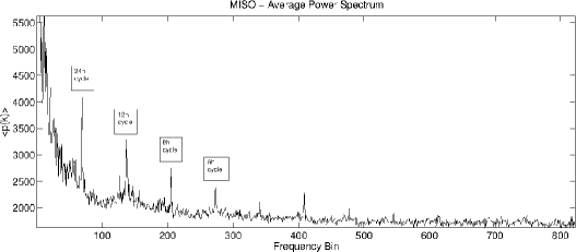
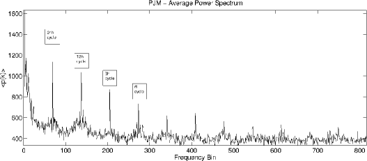
Figure 2: Average power spectrum of MISO (top) and PJM (bottom) DA MCC prices, obtained through a Fast Fourier Transform with averaging over all the nodes in each market. The power spectrum has been calculated from a time series of 1632 hours with sample rate of one hour.

In order to investigate the properties of the fluctuations of the prices, we next analyze the scaling properties using a Hurst exponent approach (Hurst (1951), Mandelbrot et al. (1997)). The Hurst exponent and its generalizations have been used to study financial market behaviours (for an introduction see Beran (1994) and Baillie (1996)). Its importance has been stressed in the last decade in a series of papers (Di Matteo et al. (2003), Bouchaud et al. (2004), Di Matteo et al. (2005), Lillo et al. (2004), Farmer et al. (2004), Bartolozzi et al. (2007), Barunik et al. (2010), Morales et al. (2012), Barunik et al. (2012), Morales et al. (2013), Kantelhardt et al. (2001), Duan and Stanley (2010)), and it has been used as a tool for quantifying the different degree of development and efficiency of various financial markets (Di Matteo et al. (2005)). Multi-scaling has been investigated also through de-trended fluctuation analysis (see for instance Kantelhardt et al. (2001), Uritskaya and Uritsky (2015) and references therein). In this paper we use the Generalized Hurst Exponent (GHE) approach.

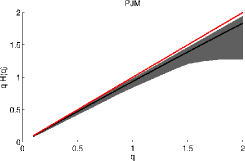
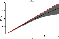
Figure 3: Analysis of the exponent $qH(q)$ in Eq. (2) for PJM (left) and MISO (right). The red line represents the $y=x$ line, and the black line is the average over the market of the function $qH_{i}(q)$. The shaded area represents the minimum and the maximum over the market. This figure shows that in MISO market the multi-fractal behaviour is more pronounced than in PJM.

The GHE is a tool used to study the statistical and scaling properties of time series. The scaling is characterized by an exponent $H(q)$ which is commonly associated with the long-term statistical dependence of the series. It is defined from the scaling of the q-th order moments of the distribution of increments (Di Matteo (2007), Di Matteo et al. (2003))

$$K_{q}(\tau)=\frac{\langle|X(t+\tau)-X(t)|^{q}\rangle}{\langle|X(t)|^{q}\rangle}\approx\Big{(}\frac{\tau}{\nu}\Big{)}^{q\ H(q)}$$ (2)

where the time interval $\tau$ can vary between $\nu$ and $\tau_{max}$, and $X(t)=cumsum(S(t))$ is the cumulative sum of the time series of interest $S(t)$, and $\nu$ is the sampling rate.

Within this framework, two kinds of processes can be distinguished: (i) a process where $H(q)=H$ is constant and independent of $q$; and (ii) a process with $H(q)$ not constant. The first case is characteristic of uni-scaling or uni-fractal processes and the scaling behaviour is determined from a unique constant $H$ that coincides with the Hurst coefficient or the self-affine index. This is the case for self-affine processes where $q\ H(q)$ is linear ($H(q)=H$) and fully determined by its index $H$. In the second case, when $H(q)$ depends on $q$, the process is commonly called multi-scaling (or multi-fractal) and different exponents characterize the scaling of different $q$-moments of the distribution. The Hurst exponent is related with the the scaling behavior observed in power spectra $\tilde{X}(k)\approx k^{-\beta}$ by $\beta=1+2H(2)$ (Di Matteo et al. (2003)).

It was noticed in (Di Matteo et al. (2003)) that the Hurst exponents evaluated using Eq. (2) do not strongly depend on the choice of detrending procedure used on the time series or on $\tau$ if this is taken sufficiently large. For the present paper we have verified that using detrendings over time windows of size $\delta t\in[6,12]$ hours, the changes of the values of the Hurst exponents were consistently below 10%.

We analyze the values of the Hurst exponents for the PJM and MISO cumulative time series i.e., we evaluate the Hurst exponent on $X(t)=cumsum(S(t))$, where $S(t)$ are the DA MCC prices. This approach is justified by the fact that in the Day-Ahead market, participants place bids one day ahead for each hour, and thus the cumulative sum of the time series is the real return as a function of time. In Fig. 3 we show the multi-scaling behavior in these markets by plotting the average quantity $qH(q)$ in Eq. (2) (dark line) together with the shaded area representing the standard deviation, and observing that these curves are below their linear trend. Fig. 3 shows that prices in both markets exhibit strong multi-fractal behaviour, although this phenomenon is more pronounced in MISO. These results are in line with (Bottazzi et al. (2012)) for the case of North-European electricity markets, and can be attributed to the fact that electricity is not economically storable.

A snapshot of the distribution of the Hurst exponent $H(1)$ is shown in Fig. 4, where we plot a histogram of $H(1)$ evaluated over the whole time series ($\delta h\approx 1600$). We observe that $H(1)\in[0.84,0.98]$ in PJM and $H(1)\in[0.85,0.99]$ in MISO, strongly deviating from the expected value of a Brownian motion, $H=0.5$. Comparing to $H(q)$ for $q=2$, in Fig. 5 we plot the histogram of $H(2)$ evaluated on the whole time series for each market, observing that $H(2)\in[0.65,0.95]$ in PJM, and $H(2)\in[0.8,0.96]$ in MISO. This shows that the Hurst exponent is indeed not constant with $q$, and in particular in the case of PJM, $H(2)$ is clustered around lower values than $H(1)$. For both $H(1)$ and $H(2)$, the generalized Hurst exponents diverge dramatically from the Brownian motion value $H=0.5$.

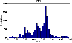
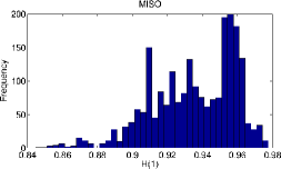
Figure 4: Descriptive statistics of the Hurst exponent $H(1)$, evaluated on the whole time series for each node, for PJM (left) and MISO (right), and for $\tau_{max}=19$ days and averaged over the whole time series.

Let us now introduce an extra parameter: the size, $\delta h$, of the moving windows on which we calculate the generalized Hurst exponents dynamically. We observed that the Hurst exponents computed on short ($\delta h=50$ hours) and long ($\delta h\approx 1600$ hours) time windows have comparable results. The dependence and importance of the choice of $\delta h$ for forecasting will be addressed specifically in the next section.

To begin with, we evaluate the Hurst exponents dynamically in a moving window of length $\delta h=50$. In Fig. 6 and Fig. 7, the black line is the average generalized Hurst exponent, for $H(1)$ and $H(2)$ evaluated on the real and filtered signal. In the latter case, we consider the signal with the frequencies which dominate the power spectrum subtracted (in particular, the 6h, 8h, 12h and 24h components). The average is taken over the nodes $i$ in the market, i.e., $\langle H_{i}(q)\rangle=\frac{1}{N}\sum_{i=1}^{N}H_{i}(q)$. See (Morales et al. (2013)) for a similar analysis performed on stock market data. The use of a short time window with $\delta h=50$ hours will be further motivated in the next section, where we will suggest the use of this training window to minimize forecast errors. It is also interesting to note that even if evaluated on such a short window, the values of these exponents appear to be in the same ranges as those evaluated on the whole time series.

For both PJM and MISO, the Hurst exponent is subject to rather strong fluctuations and spiky behaviour. We note that the latter is rather attenuated when we consider the signal from which the cyclic components have been removed, but still the Hurst exponents oscillate in the range $H(1)\approx 0.6-0.9$ and $H(2)\approx 0.5-0.85$ for both markets, which confirms the persistence of the fluctuations. Even after the signal has been filtered, we note that some abrupt transitions occur for both $H(1)$ and $H(2)$. Further, in Fig. 6 we show that there are changes in $H(1)$ and $H(2)$ which are coherent across the entire market. In the case of some of these sharp movements, we could identify specific weather events which could have potentially triggered this coherent behaviour. For instance, in the case of PJM, the sharp transition occurring at $t\approx 880$h corresponds to a severe snowfall occurring in Pennsylvania on the 5th of February 2014. We thus argue that the behaviour of the fluctuations can be interestingly connected to specific exogenous factors.

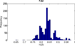
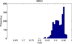
Figure 5: Descriptive statistics of the Hurst exponent $H(2)$, evaluated on the whole time series for each node, for PJM (left) and MISO (right), and for $\tau_{max}=19$ days.

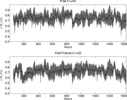
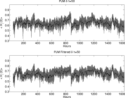
Figure 6: Average H(1) and H(2) exponents for PJM evaluated dynamically, with and without filtering, on a moving time window of $\delta h=50$ hours. The dark line represents the average value across the market, meanwhile the shadowed area represents the standard deviation. We observe that for both filtered and unfiltered time series the average value of $H(1)$ oscillates around high values of the Hurst ($\approx 0.5-0.9$), although some nodes occasionally have values below $H=0.5$, thus exhibiting also anti-persistent behavior. $H(2)$ is consistently lower than $H(1)$, with $H(2)\approx 0.45-0.82$. In general both exponents differ strongly from the Brownian motion expected value of $H=0.5$. We note that due to the short time window on which the Hurst is calculated here, these values are consistently lower than the one evaluated on the whole time series, as in Fig. 4. In addition, many of the spikes observed in the unfiltered signal disappear or are attenuated in the filtered case.

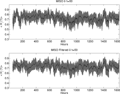
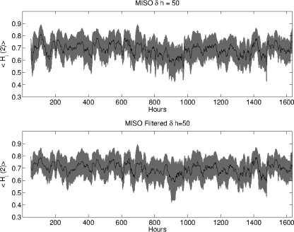
Figure 7: Average H(1) and H(2) exponents for MISO, with and without filtering, calculated on a moving time window of $\delta h=50$ hours, as in Fig. 6. The dark line represents the average value across the market, and the shadowed area represents the standard deviation. We observe that for both markets the average values of $H(1)$ and $H(2)$ oscillate around high values, $H(1)\approx 0.5-0.9$ and $H(2)\approx 0.5-0.8$, and $H(2)$ has a systematically lower value than $H(1)$. Finally, the filtered signal shows less cyclicality and spiky behavior.

4 Generalized Hurst exponent and trends

Several studies have suggested that the Hurst exponent might be a measure of predictability of time series in stock markets (for instance Lillo et al. (2004), Farmer et al. (2004)) and connected it to the efficient market hypothesis. It has been studied in detail in different models of stock markets as a measure of returns predictability in (Duan and Stanley (2010)) and (Mitra (2012)), and as a predictor of forecast quality for neural networks models in (Qian et al. (2007)). The relation between the Hurst exponent and the efficient market hypothesis has also been studied in (Eom et al. (2008), Eom et al. (2008)). The predictability of Canadian electricity market prices using detrendend fluctuations is analysed in (Uritskaya and Uritsky (2015)). There is also a large literature on the predictability of electricity prices, for examples see Aggarwal et al. (2009), Moest et al. (2010), Benth et al. (2012), Wang et al (2013). Our focus will be on applying the Generalized Hurst exponent method for forecasting purposes. In order to do so, we introduce a simple linear regression model and measure the dependence of the forecast error on the Generalized Hurst exponent evaluated dynamically for each time series.

4.1 The model

Consider the simplest forecast method, a linear regression model. In particular, for each time-series $S_{i}$, we extrapolate the next $p$-points by means of a linear regression performed on the previous $\delta h$ points: $\hat{S}_{i}(t+p)=\beta_{1}p+\beta_{0}$, with the intercept fixed at the last observation $\beta_{0}=S(t)$. It is well know that linear regression suffers from various problems, since it relies on the normal distribution of errors, does not take into account heteroscedasticity, and does not capture non-linear or chaotic patterns. Our goal here is to test the relationship between the Hurst exponent and the persistence of a trend as measured by a linear model. These regressions are performed for each node in the market independently. For each prediction, one can associate an error and two independent datapoints given by the values of the Generalized Hurst, $H_{i}(1)$ and $H_{i}(2)$ evaluated over the training window. More precisely, we will study the relationship between forecast error and these Hurst exponents.

4.2 Results

We introduce the forecast error, $E_{i}(t,p)=|\hat{S}_{i}(t+p)-S_{i}(t+p)|$, with implicit training window $\delta h$. We then compare the forecast error at time $t$ with the values of the Generalized Hurst exponents $H_{i}(1)$ and $H_{i}(2)$ computed in the time window $[t-\delta h,t]$ for the time series $i$. Given the prediction window $\delta h$, there are $(1632-\delta h)\times N$ errors and Generalized Hurst values, where $N$ is the number of time series in the market, and 1632 is the number of hours available for our analysis. In Fig. 8 we plot the density of points in the semi-log scatter plot of Generalized Hurst exponents versus forecast error for $\delta h=50$, evaluated at $p=1$ both for PJM (left) and MISO (right), together with the best fit, for both $q=1$ (top) and $q=2$ (bottom). Similar results were obtained also for $\delta h=50-100$ hours. We observe a negative dependence between the values of the Generalized Hurst exponent and the prediction error, implying that for higher Hurst exponents one has better forecasting power. This indicate that $H(q)$ and $E(H(q))$ have a functional dependency: $E(H(q))\approx E_{0}10^{cH(q)}$ where $c$ is the slope in the log-linear fit.

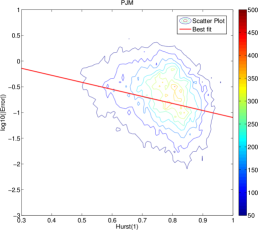
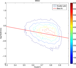
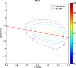
Figure 8: Density plot of mean squared forecast error versus $H(q)$ for PJM (left) and MISO (right), for $q=1$ (top) and $q=2$ (bottom), for the case of a linear regression forecast and with training window $\delta h=50$. This shows that the dependence on the Hurst is negative. The line is given by the linear fit $E(H(q))\approx E_{0}10^{cH(q)}$, with $E_{0}$ the intercept and $c$ is the slope in the log-linear plot.

In addition, we study the effect of the seasonal components shown in Fig. 2 by taking the filtered time series, in which the $24h$, $12h$, $8h$ and $6h$ components have been removed. The results for the linear fit slope $c$ for both original and filtered time series are reported in Fig. 9 (top) and Fig. 9 (bottom) for $\delta h=50$ hours, for $H(1)$ and $H(2)$.

We observe that the results are strongly affected by filtering the time series. The dashed lines (filtered) are above the full line (unfiltered), showing the importance of the strongly cyclical components for the trend of the time series as measured by the Hurst exponents. These results apply, qualitatively, also to the case of the MISO market, where we observe smaller values of $c$ in absolute value, but similar patterns in the curve $c(p)$ shown in Fig. 9.

This analysis suggests that the Generalized Hurst is a good estimator of trend persistence in the case of the electricity markets considered here, and we note that in general $H(2)$ is a better estimator than $H(1)$. In addition, pries in PJM are more predictable than in MISO.

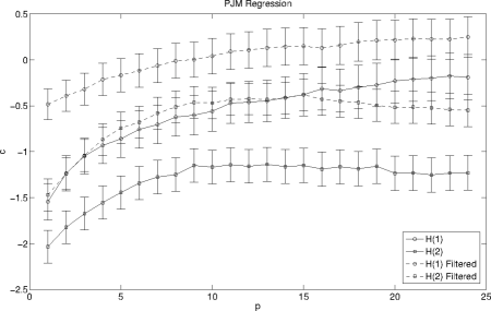
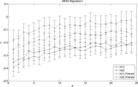
Figure 9: Plot of the slopes $c$ versus the prediction lag $p$ for PJM (left) and MISO (right) as a function of $H(1)$ and $H(2)$, both for filtered (dashed line) and unfiltered (full line) signals and for $\delta h=50$ hours.

5 Conclusions

In this paper we studied the Generalized Hurst exponent for the Day-Ahead Marginal Congestion Cost components of electricity prices in two North American wholesale electricity markets. We observed that these prices exhibit strong multi-scaling behaviour and deviation from Brownian motion. We also observed that in the power spectrum of the time series several peaks associated to daily cycles can be identified. We found that the values of the Generalized Hurst exponents, $H(1)$ and $H(2)$, are are clustered between $0.7$ and $0.8$ for both markets. To our knowledge, this is the first analysis of Generalized Hurst exponents performed for these electricity markets. Doing a dynamic analysis of these exponents using moving windows of $50$ hours, we found that the generalized Hurst exponents have values which are consistently related with those evaluated on longer time windows, and have coherent market movements.

We have also shown that the Generalized Hurst exponent is a good estimator of the persistence of trends in the time series if the strongly cyclical components are taken into account, supporting the hypothesis that for higher Hurst exponents ($>\approx 0.5$) the fluctuations are trend supporting and thus simple linear models can be used to perform predictions. In general the results are different depending on the training window. In fact there is a negative correlation between the Hurst exponents and the forecast errors of the regressions, and this correlation depends on the size of the forecast horizon. Using a training window between $50-100$ hours provides the best results. In analogy to the case of stock markets, where the Hurst exponent has been connected to the efficient market hypothesis (Di Matteo et al. (2003), Lillo et al. (2004), Di Matteo et al. (2005)), we have observed that indeed the Hurst exponent can be connected to the error in the prediction of returns.

Aknowledgements

F.C. would like to thank Francois Lafond and Doyne J. Farmer for comments at the beginning of this work. The work of F.C., J.R., C. U. and A. A. was supported by Invenia Technical Computing corporation. TA acknowledges support of the UK Economic and Social ResearchCouncil (ESRC) in funding the Systemic Risk Centre [ES/K002309/1]. TDM wishes to thank the COST Action TD1210 for partially supporting this work. F.C. would like to also thank LIMS for hospitality meanwhile carrying out this study.

References

- Loskow (2008) P. Loskow, Lessons Learned from Electricity Market Liberalization The electricity Journal, Special Issue on the Future of Electricity, pp. 9-42, 2008
- Hurst (1951) H. Hurst, Long Term Storage Capacity of Reservoirs. Transactions of the American Society of Civil Engineers 116, 770-799. (1951)
- Hogan (2008) W. H. Hogan, Electricity Market Structure and Infrastructure, Acting in Time on Energy Policy Conference (2008)
- F. Caravelli et al. (2015) F. Caravelli et al., PJM and MISO electricity markets price data, figshare, http://dx.doi.org/10.6084/m9.figshare.1412608 (2015)
- Liu (2009) H. Liu, L. Tesfatsion, A. A. Chowdhury, Locational Marginal Pricing Basics for Restructured Wholesale Power Markets, Power and electricity Society General Meeting. PES ’09. IEEE (2009)
- Brown (2012) P. Brown, U.S. Renewable Electricity: How Does Wind Generation Impact Competitive Power Markets, Congressional Research Service 7-5700, Report 42818 (2012)
- Popova (2004) J. Popova, Spatial Pattern in Modeling Electricity Prices: Evidence from the PJM Market, 24th USAEE and IAEE North American Conference, July 8-10, Washington, DC (2004)
- Weron (2006) R. Weron, Modeling and Forecasting Electricity Loads and Prices: A Statistical Approach, Joh Wiley & Sons, Southern Gate (UK)
- Kwon (2012) R. H. Kwon, D. Frances, Optimization-Based Bidding in Day-Ahead Electricity Auction Markets: A Review of Models for Power Producers, Handbook of Networks in Power Systems I, Electricity Systems 2012, pp 41-59
- Beran (1994) J. Beran, Statistics for Long-Memory Processes. Chapman Hall (1994)
- Mandelbrot et al. (1997) B.B. Mandelbrot, A. Fisher, and L. Calvet. The multifractal model of asset returns. Cowles Foundation discussion paper no. 1164, Yale University (1997)
- Kantelhardt et al. (2001) J.W. Kantelhardt, S.A. Zschiegner, E. Koscielny-Bunde, S. Havlin, A. Bunde, H.E. Stanley, The fractal detrended fluctuation analysis of nonstationary time series, Physica A (2001) 87: 316.
- Baillie (1996) R.T. Baillie, Long-memory processes and fractional integration in econometrics. Journal of Econometrics 73, 5-59 (1996)
- Bouchaud et al. (2004) J.-P. Bouchaud, Y. Gefen, M. Potters, and M. Wyart , 2004, Fluctuations and response in financial markets: the subtle nature of “random” price changes, Quantitative Finance 4 176-190
- Lillo et al. (2004) F. Lillo, J. D. Farmer, The long memory of the efficient markets, Studies in Nonlinear Dynamics and Econometrics. Volume 8, Issue 3, ISSN (Online) 1558-3708
- Farmer et al. (2004) J.D. Farmer, F. Lillo, On the origin of power-law tails in price fluctuations. Quantitative Finance 4, C7-C11 20-26. (2004)
- Di Matteo et al. (2005) T. Di Matteo, T. Aste, M. M. Dacorogna, Long term memories of developed and emerging markets: using the scaling analysis to characterize their stage of development, Journal of Banking & Finance 29/4 (2005) 827-851
- Qian et al. (2007) B. Qian, K. Rasheed, Hurst exponent and financial market predictability, IASTED conference on Financial Engineering and Applications (FEA 2004). pp. 203-209
- Duan and Stanley (2010) W.-Q. Duan, H. E. Stanley, Volatility, irregularity, and predictable degree of accumulative return series, PRE 81, 066116 (2010)
- Eom et al. (2008) C. Eom, G. Oh, W.-S. Jung, Relationship between efficiency and predictability in stock price change, Physica A 387 (2008) 5511-5517
- Eom et al. (2008) C. Eom, G. Oh, W.-S. Jung, Hurst exponent and prediction based on weak-form efficient market hypothesis of stock markets, Physica A 387 (2008) 4630-4636
- Barunik et al. (2010) J. Barunik, L. Kristoufek, On hurst exponent estimation under heavy-tailed distributions, Physica A 389 (2010) 3844-3855
- Barunik et al. (2012) J. Barunik, T. Aste, T. Di Matteo, R. Liu, Understanding the source of multifractality in financial markets, Physica A 391 (2012) 4234-4251; J. Barunik, T. Di Matteo, R. Gramatica, T. Aste, Dynamical generalized Hurst exponent as a tool to monitor unstable periods in financial time series, Physica A 391 (2012) 3180-3189
- Lo (1991) A. W. Lo, Long-Term Memory in Stock Market Prices, Econometrica, Vol. 59, No. 5 (1991), pp. 1279-1313
- Morales et al. (2013) R. Morales, T. Di Matteo, T. Aste, Non stationary multifractality in stock returns, Physica A 392 (2013) 6470-6483.
- Liu (2012) R. Liu, Understanding the source of multifractality in financial markets, Physica A, 391 (2012) 4234?4251.
- Morales et al. (2012) R. Morales, T. Di Matteo, R. Gramatica, T. Aste, Dynamical Hurst exponent as a tool to monitor unstable periods in financial time series, Physica A, 391 (2012) 3180-3189.
- Bartolozzi et al. (2007) M. Bartolozzi, C. Mellen, T. Di Matteo, and T. Aste, Multi-scale correlations in different futures markets, Eur. Phys. J. B 58 (2007) 207-220.
- Di Matteo et al. (2005) T. Di Matteo, T. Aste and M. M. Dacorogna, ”Long term memories of developed and emerging markets: using the scaling analysis to characterize their stage of development”, J. of Banking and Finance 29/4 827-851 (2005).
- Di Matteo (2007) T. Di Matteo, “Multi-scaling in finance”, Quantitative Finance, Vol. 7, No. 1 (2007)
- Di Matteo et al. (2003) T. Di Matteo, T. Aste and M. M. Dacorogna, ”Scaling behaviors in differently developed markets”, Physica A 324 (2003) 183-188.
- Mitra (2012) S. K. Mitra, “Is Hurst Exponent Value Useful in Forecasting Financial Time Series?”, Asian Social Science Vol. 8, No. 8 ( 2012)
- Uritskaya and Uritsky (2015) O. Y. Uritskaya, V. M. Uritsky,“Predictability of price movements in deregulated electricity markets”, Energy Economics 49 (2015)
- Aggarwal et al. (2009) S. K. Aggarwal, L. M. Saini, A. Kumar, “Electricity price forecasting in deregulated markets: A review and evaluation”, International Journal of Electrical Power & Energy Systems 31 (1) (2009) 13-22.
- Moest et al. (2010) D. Moest, D. Keles, “A survey of stochastic modelling approaches for liberalised electricity markets”, European Journal of Operational Research 207 (2) (2010) 543-556
- Benth et al. (2012) F. E. Benth, R. Kiesel, A. Nazarova, “A critical empirical study of three electricity spot price models”, Energy Economics 34 (5) 1589-1616 (2012)
- Bottazzi et al. (2012) G. Bottazzi, S. Sapio, A. Secchia, “Some statistical investigations on the nature and dynamics of electricity prices”, Physica A 355, 54-61 (2005)
- Wang et al (2013) F. Wang, G. Liao, J. Li, R. Zou, W. Shi, “Cross-correlation detection and analysis for California’s electricity market based on analogous multifractal analysis”, Chaos 013129 (2013)
- Frances (2004) P. H. Frances, A concise introduction to Econometrics, Cambridge University Press, Cambridge UK (2004)
- Bohn et al (1984) R. Bohn, M. Caramanis, F. Schweppe, “Optimal Pricing in Electrical Networks over Space and Time”, The RAND Journal of Economics 15 (3) (1984) 360-376