Noise-Induced Transitions in Optomechanical Synchronization
Abstract
We study how quantum and thermal noise affects synchronization of two optomechanical limit-cycle oscillators. Classically, in the absence of noise, optomechanical systems tend to synchronize either in-phase or anti-phase. Taking into account the fundamental quantum noise, we find a regime where fluctuations drive transitions between these classical synchronization states. We investigate how this “mixed” synchronization regime emerges from the noiseless system by studying the classical-to-quantum crossover and we show how the time scales of the transitions vary with the effective noise strength. In addition, we compare the effects of thermal noise to the effects of quantum noise.
I Introduction
The field of cavity optomechanics deals with systems where light in an optical cavity couples to mechanical motion Aspelmeyer et al. (2014). Recent experimental progress allows to move on from the investigation of a single optomechanical system to several coupled optomechanical systems. There are already first experiments that involve a few mechanical and optical modes Hill et al. (2012); Dong et al. (2012); Grudinin et al. (2010); Bahl et al. (2012), exploiting them for wavelength conversion, phonon lasing and efficient cooling. Such few-mode optomechanical setups have been the subject of an increasing number of theoretical proposals, on topics such as efficient state transfer Wang and Clerk (2012), two-mode squeezing Woolley and Clerk (2014), back-action evading measurements Woolley and Clerk (2013), entanglement Paternostro et al. (2007); Deng et al. (2014); Wang et al. (2015) or Landau-Zener dynamics Heinrich et al. (2010); Wu et al. (2013).
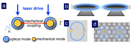
Larger arrays may be implemented using a variety of settings, such as coupled disks Zhang et al. (2012) (Fig. 1(b)) or optomechanical crystal structures Maldovan and Thomas (2006); Eichenfield et al. (2009); Safavi-Naeini et al. (2010); Gavartin et al. (2011); Laude et al. (2011); Safavi-Naeini et al. (2014) (Fig. 1(d)). Optomechanical arrays have also attracted attention from a theoretical point of view. They have been studied in the context of slowing light Chang et al. (2011), Dirac physics Schmidt et al. (2015a), reservoir engineering Tomadin et al. (2012), artificial magnetic fields for photons Schmidt et al. (2015b), heat transport Xuereb et al. (2015), and topological phases of sound and light Peano et al. (2014). Furthermore, multi-membrane systems Bhattacharya and Meystre (2008); Xuereb et al. (2012, 2013, 2014) were studied theoretically, considering for instance long-range interactions and dynamics.
Most notably, optomechanical arrays provide a platform to study synchronization of mechanical oscillators. This was initially pointed out in Ref. Heinrich et al. (2011). Synchronization is a well known phenomenon in many different branches of science Kurths et al. (2001) and typically arises whenever there are stable limit-cycle oscillations. However, we note that synchronization-like phenomena have been recently studied also in the context of linear oscillators dissipating into a common bath Giorgi et al. (2012). Optomechanical systems exhibit a Hopf bifurcation and can be optically driven into mechanical limit-cycle oscillations Höhberger and Karrai (2004); Kippenberg et al. (2005); Marquardt et al. (2006); Metzger et al. (2008). These self-oscillations have also been analyzed theoretically in the quantum regime Ludwig et al. (2008); Qian et al. (2012); Lörch et al. (2014). The theoretical description of the synchronization dynamics in optomechanical arrays has initially focussed on the classical regime Heinrich et al. (2011); Holmes et al. (2012). More recent insights into this regime include the pattern formation of the mechanical phase field in larger optomechanical arrays Lauter et al. (2015). In the quantum regime, it was found Ludwig and Marquardt (2013) that quantum noise can drive a sharp nonequilibrium transition towards an unsynchronized state in an extended array, even for optomechanical systems with identical frequencies. Further general insights into quantum synchronization were gained in a model system of one van-der-Pol oscillator coupled to an external drive Walter et al. (2014a) or two coupled van-der-Pol oscillators Walter et al. (2014b), which can serve as a rough approximation to an actual optomechanical system. A number of more recent works have explored quantum synchronization on the more conceptual level Hermoso de Mendoza et al. (2014), as well as in various other physical systems, such as e.g. trapped atoms and ions Lee and Sadeghpour (2013); Lee et al. (2014); Hush et al. (2015); Xu et al. (2014), qubits Zhirov and Shepelyansky (2009); Savel’ev et al. (2012); Giorgi et al. (2013), and superconducting devices Hriscu and Nazarov (2013). The relation of synchronization and correlations in the quantum-to-classical transition was studied in a system of coupled cavities containing a non-linearity Lee et al. (2013). Notably, it is still challenging to define a good measure for quantum synchronization Mari et al. (2013); Ameri et al. (2015); Hush et al. (2015).
Only recently synchronization of two nanomechanical oscillators in the classical regime was demonstrated experimentally. This has been achieved using optomechanical systems with coupled micro-disks Zhang et al. (2012) (Fig. 1(b)), as well as in an experiment involving an optical racetrack cavity coupled to two mechanical oscillators Bagheri et al. (2013) (Fig. 1(c)), and also in a setup using nanoelectromechanical systems Matheny et al. (2014). In a recent first step towards larger arrays, up to seven optically coupled micro-disks were used to demonstrate the expected phase noise reduction due to synchronization Zhang et al. (2015). This phase noise reduction with the number of coupled systems is considered to be one of the main prospects of synchronized nanomechanical arrays. Indeed, recognized from the very beginning with the synchronization of pendulum clocks Huygens (1673), synchronization has the potential to improve time-keeping and frequency stability. Examples where different types of synchronization have been applied or suggested for application are for frequency stabilization of high power lasers by coupling to a more stable, low power laser Buczek et al. (1972) and for secure communication in connection with chaos Cuomo et al. (1993). For a more complete overview and also the many applications to biology see e.g. Kurths et al. (2001); Rosenblum et al. (2003); Dörfler et al. (2014).
In this work we study the effects of quantum and thermal noise on the synchronization of two optomechanical systems. We focus on a bistable synchronization regime that either exists already in the absence of noise, or is induced by it. Bistabilities in quantum systems have been investigated before Dykman et al. (1988); Peano et al. (2006); Ghobadi et al. (2011) and noise-induced bistabilities are known in several other systems in biology and chemistry Samoilov et al. (2004); Biancalani et al. (2014); Houchmandzadeh et al. (2015), as well as in physics Fichthorn et al. (1989); Kim et al. (1996); Residori et al. (2001). We find and discuss noise-induced bistable behaviour now in the context of optomechanical (quantum) synchronization.
This manuscript is organized as follows: We begin with a brief review of classical synchronization in the absence of noise, Sec. II. Then, we introduce our model in Sec. III, explain our methods in Sec. IV, and state our main results in Sec. V. We note that both quantum and thermal noise lead to similar effects, but start out with the investigation of quantum noise effects. Therefore, in Sec. VI, we simulate the full quantum behaviour of the system, in contrast to the previous investigation presented in Ref. Ludwig and Marquardt (2013). We find a regime of “mixed” synchronization with two stable synchronization states, and we explore its classical-to-quantum crossover in Sec. VII. In Sec. VIII, we give an overview of the different synchronization regimes. Finally, in Sec. IX, we discuss the effects of thermal noise as compared to quantum noise. This is important to gauge the potential of observing the quantum noise effects discussed here in future experiments.
II Brief review: Classical Synchronization of optomechanical Oscillators
In this section we briefly review the concepts of classical synchronization of optomechanical systems in the absence of noise. This will set the stage for the discussion of our results on synchronization in the presence of thermal and quantum noise.
A widely studied model for synchronization is the Kuramoto model Kuramoto (1975); Acebrón et al. (2005), which describes a set of coupled phase oscillators. Each phase oscillator has a phase and an intrinsic frequency , and couples to the other oscillators via the phase difference. For two oscillators, the two corresponding phase equations collapse into one equation for the relative phase ,
| (1) |
The two oscillators are synchronized if their respective phase velocities become equal, , i.e. . From Eq. (1) one finds the synchronization threshold: The two oscillators are synchronized if the coupling exceeds the natural frequency difference, . Following this condition, oscillators with identical intrinsic frequencies are always synchronized. There is only a single stable value of in the synchronized regime. For , this value approaches zero, , whereas for .
Although synchronization appears in a large range of systems which are very different in terms of microscopic parameters, their behaviour can often be captured by effective phase equations of the Kuramoto-type Kurths et al. (2001); Acebrón et al. (2005). In the context of optomechanics, the mechanical motion of a single optomechanical system near the Hopf bifurcation can be described with a phase and an amplitude equation Marquardt et al. (2006). Starting from these equations, an effective Kuramoto-type model for coupled optomechanical systems has been derived Heinrich et al. (2011). This model describes arrays of arbitrary many optomechanical cells with arbitrary intrinsic frequencies. For two oscillators, the phase equations of this model reduce, again, to a single equation for the phase difference
| (2) |
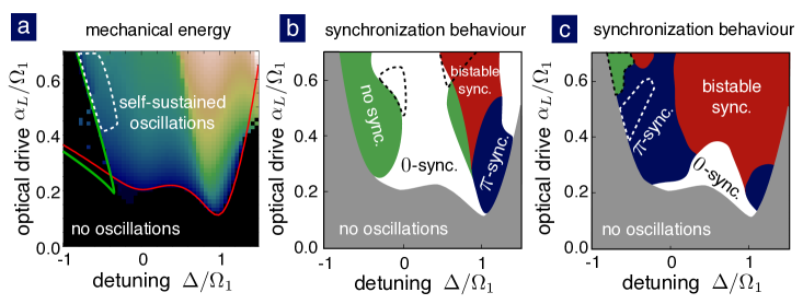
Here, and are effective parameters depending on the microscopic parameters of the underlying optomechanical systems Heinrich et al. (2011); Ludwig and Marquardt (2013). Note that the -term was added to the model only later Ludwig and Marquardt (2013), and accounts for the change of the intrinsic frequencies with the mechanical oscillation amplitude. Recently, the resulting full Hopf-Kuramoto model has been used to study pattern formation in 2D arrays of optomechanical systems Lauter et al. (2015). In contrast to the original Kuramoto model Eq. (1), the optomechanical Hopf-Kuramoto model Eq. (2) includes a term that involves . Rewriting Eq. (2) in terms of an effective potential, Heinrich et al. (2011), this term corresponds to the appearance of a second minimum close to which can co-exist with the minimum close to . This allows optomechanical systems to synchronize not only in-phase (-synchronization), , but also anti-phase (-synchronization), . For the effective potential there are three different possibilities, depending on the parameters and : (i) It has a single minimum close to which leads to -synchronization only, (ii) it has a single minimum close to which leads to -synchronization only, or (iii) both minima appear simultaneously in the effective potential, such that the initial conditions determine whether - or -synchronization occurs. These three regimes are schematically shown in Fig. 2(b) and (c) and discussed in Sec. III.
In general, for optomechanical arrays an effective potential for the phases does not exist Lauter et al. (2015). However, in the case of two oscillators only, the system can be described with one degree of freedom, i.e. the relative phase , and an effective potential for can always be constructed. Below, we make use of the existence of this effective potential to give an intuitive understanding of synchronization even in the presence of noise.
III Model
We now introduce the model that we investigate throughout the rest of this manuscript. We study two optomechanical systems which are mechanically coupled, see Fig. 1(a). Our goal is to analyze the synchronization behaviour in the presence of quantum and thermal noise. Each optomechanical system consists of a driven optical mode () coupled to a mechanical mode () via radiation pressure. In a frame rotating at the laser drive frequency , the Hamiltonian of each optomechanical system is
| (3) |
Here, denotes the detuning from the cavity resonance , is the resonance frequency of the mechanical mode, denotes the optomechanical single photon coupling strength, and is the laser driving strength. Note that the optical and the mechanical systems experience damping at a rate and , respectively, and these are described by adding to the Hamiltonian a system-bath coupling in the usual manner: .
Driving a single optomechanical system with a blue-detuned laser causes self-oscillations of the mechanical resonator when the optomechanically induced negative damping is larger than the intrinsic damping of the oscillator Marquardt et al. (2006). In Fig. 2(a) we show this threshold of self-oscillations. Throughout this work we only consider parameters such that the single optomechanical systems are above this threshold. Self-oscillations at occur due to the static optomechanical shift which leads to an effective blue detuning, i.e. . These limit-cycle oscillations, in the absence of noise, can effectively be described by a fixed amplitude and a phase and are treated as a prerequisite for synchronization throughout this work. We consider two self-oscillating optomechanical systems that are coupled mechanically with strength , such that the total Hamiltonian of the system (except for the dissipative part) reads
| (4) |
Experimentally, this coupling between the mechanical oscillators can also be mediated by an optical coupling, cf. Fig. 1(b)-(d). In recent experiments Zhang et al. (2012); Bagheri et al. (2013); Zhang et al. (2015), a single joint optical mode was employed to couple the mechanical oscillators. However, this mode served a dual purpose in creating the limit cycles via a blue-detuned drive and providing the coupling. Using an additional, independently driven optical mode for the coupling would allow to tune the effective (optically induced) coupling independently from the laser drive used to create the limit cycles.
In experiments, the typical mode of operation is to have the two optomechanical oscillators at slightly different intrinsic mechanical frequencies. These start out un-synchronized but can synchronize upon changing some parameter (e.g. the laser drive strength, the detuning, or potentially the coupling). This is schematically shown in Fig. 2(b), where we indicate the synchronization regimes in the absence of noise. In accordance to the Hopf-Kuramoto model, cf. Sec. II, there are unsynchronized regions and three different synchronization regimes: (i) -synchronization, (ii) -synchronization, and (iii) classical bistable synchronization where the type of synchronization depends on the initial conditions. Note that for different intrinsic mechanical frequencies, , the relative phase is not exactly or but only close to one of these values and varies within the synchronization regime.
However, in the presence of noise it is already interesting to investigate the behaviour even for identical frequencies. In particular, for large-scale optomechanical arrays of identical oscillators, it has been found that there is a synchronization transition as a function of noise strength Ludwig and Marquardt (2013). Moreover, in the present article we will focus on noise-induced transitions between various synchronization states. The observation of this physics does not rely on whether there is an actual synchronization transition at lower values of the coupling. Therefore, in most of our analysis, we will focus on identical systems, i.e. we assume all the parameters to be equal in both systems. In Fig. 2(c) we schematically show the synchronization regimes for identical optomechanical systems and for a larger mechanical coupling than in Fig. 2(b), but still in the absence of noise. It is important to note that both the mechanical detuning and the coupling have an influence on this diagram: Not synchronized regions can become synchronized and synchronization regime borders are shifted.
We will comment on the dynamics of two coupled optomechanical oscillators with different frequencies in Sec. VIII.
IV Methods
In this work we use Langevin equations and quantum jump trajectories to study the system described by Hamiltonian (4) in the presence of (quantum) noise. Here we want to briefly present both approaches and discuss their respective advantages and problems.
Most of our results are computed with semi-classical Langevin equations. They are obtained by first deriving quantum Langevin equations from Hamiltonian (4) using input-output theory Walls and Milburn (2008). We then adopt a semi-classical approach by turning the quantum Langevin equations into classical Langevin equations for the complex amplitudes and , where the noise terms mimic the quantum-mechanical zero-point fluctuations. This can be understood as a variant of the “truncated Wigner approximation”. The semi-classical equations are:
| (5) | ||||
The corresponding equations for the second optomechanical system can be obtained from Eqs. (5) by exchanging the indices . Here, and represent the optical and mechanical input noise, given by Gaussian stochastic processes. Since complex numbers commute, they obviously cannot correctly fulfill the input-output quantum noise correlators, and . Instead, and are made to mimic quantum noise by fulfilling (and likewise for for ). This approach allows to study also large parameter ranges with relatively low computational effort.
Deep in the quantum regime it is initially not clear that these semi-classical Langevin equations describe the correct physical behaviour. In order to verify the qualitative effects observed with Langevin equations, we also present a few results obtained with quantum jump trajectories Mølmer et al. (1993); Plenio and Knight (1998), i.e. an “unraveling” of the Lindblad master equation. Applying this method, the fully quantum system is simulated on an appropriately truncated Hilbert space. Notably, it allows to work with wave functions, in contrast to the formalism of the Lindblad master equation which requires the use of density matrices. Hence, simulations of larger Hilbert spaces become feasible. In addition, quantum jump trajectories give access to additional observables, for instance the full counting statistics. For these reasons, quantum jump trajectories have been applied in many different contexts. In the field of quantum synchronization, such methods have been used to study synchronization of qubits Zhirov and Shepelyansky (2009). In the field of cavity optomechanics, they have been employed for instance to discuss QND measurements, photon statistics and single photon optomechanics Ludwig et al. (2012); Kronwald et al. (2013); Akram et al. (2013); Mirza and van Enk (2014). Another motivation is the recent experimental detection of individual phonons in optomechanical systems Cohen et al. (2015) - a step towards monitoring full quantum jump trajectories in experiments.
To explain this approach Mølmer et al. (1993); Plenio and Knight (1998), let us consider for a moment photon decay in cavity 1. The “unraveling” discussed here corresponds to the physical setup of placing a single photon detector at the output port of the cavity. At each time step , the probability of a single photon to leak out of the cavity (at temperature ) is given by . In the case of a photon loss it is detected at the output port and the wave function is updated . If no photon was lost to the environment, the wave function evolves in time according to a (non-Hermitian) Hamiltonian that is obtained by adding a term . This additional term accounts for the information gained about the system by not observing a photon Ueda et al. (1990). In both cases the state has to be normalized before proceeding to the next time step. The treatment of photon loss in cavity 2 and of phonon losses works analogously. This simulation approach naturally accounts for quantum fluctuations.
Although it would be favourable to use quantum jump trajectories throughout the whole study, this approach is only computationally feasible whenever the needed Hilbert space remains sufficiently small. This leads to severe limitations in the choice of parameters and especially gives no access to the full classical-to-quantum crossover that is studied in Sec. VII. In Ref. Ludwig et al. (2008) it has been shown for a single optomechanical system that semi-classical Langevin equations produce good agreement with the full quantum theory. A systematic comparison for two coupled optomechanical systems is not possible, since the number of required Hilbert space dimensions is squared as compared to the single optomechanical system. We comment on this in Sec. VII.1 (cf. Fig. 4(a) and the discussion below).
Note that quantum jump trajectories serve here as a numerical approach only. In experiments, single photon and phonon detection is not necessary. Instead, the mechanical oscillators could be measured using standard homodyning techniques.
V Main Results
In this section we briefly state our main results, which will be discussed in the following sections. Most notably, it is known even from the classical theory that two coupled optomechanical oscillators can be in either one of two synchronization states (with a phase difference near or near ). We find a regime of “mixed” synchronization, where transitions between - and -synchronization occur (Sec. VI). These transitions are driven by (quantum or thermal) noise and cannot be found in the classical, noiseless situation. The average residence times in the two synchronization states can differ and their ratio varies with the system parameters (Sec. VII). Investigating the classical-to-quantum transition, we find that mixed synchronization can evolve from two different regimes in the classical, noiseless limit: (i) there are already two stable synchronization states but in the absence of noise there are no transitions, (ii) there is only one stable synchronization state and only the presence of noise leads to a second stable solution. Although the first sections are devoted to the investigation of quantum noise effects, we note that we find similar effects for thermal noise acting on the mechanical resonator. However, quantitative differences remain due to the different nature of the noise source (Sec. IX). We find that quantum noise effects should dominate over thermal noise effects if the optomechanical cooperativity is sufficiently large, and a large value of is not necessarily required.
VI Multistable Quantum Synchronization
First, we start by analyzing two coupled optomechanical systems, cf. Fig. 1(a), deep in the quantum regime. Quantum jump trajectories are used to initially investigate the full quantum dynamics. In the following, we consider a small-amplitude limit cycle and a large single-photon coupling strength, . This ensures that quantum fluctuations can potentially have a large impact on the system’s dynamics. Furthermore, small photon and phonon numbers are necessary to keep the numerical simulations tractable, since they determine the size of the truncated Hilbert space.
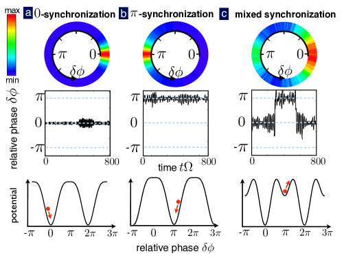
To study synchronization we focus on the relative phase between the optomechanical oscillators. Classically, allows to identify synchronization () and distinguish the different synchronization regimes (- and -synchronization). To extract the relative phase at each time step of a quantum jump trajectory, we use that the motion of the uncoupled self-oscillators in the absence of noise can effectively be described by , with an initial random phase . Thus, the correlator can be interpreted as a measure for the relative phase . In Fig. 3 we show the probability density of the relative phase obtained from the distribution of and a typical sample of the corresponding phase trajectory. We find a -synchronized regime, Fig. 3(a), where the relative phase is predominantly close to . Similarly, we find a -synchronized regime, Fig. 3(b), for different parameters. As expected, noise prevents perfect synchronization and thus the corresponding maximum in the probability density has a finite width. Likewise, the trajectories show fluctuations around either or . These two synchronization regimes have an analog in the classical, noiseless limit, cf. Sec. II. In addition, we find another regime where the probability density of the phase difference has maxima close to both and , see Fig. 3(c). The corresponding trajectory shows that in this regime transitions between the two synchronization states occur. We call this regime “mixed” synchronization. This is in contrast to the classical, noiseless result, where the system does not change its synchronization state with time, not even in the regime of bistable synchronization.
Similar to the classical, noiseless system Heinrich et al. (2011) we can understand these results in terms of an effective potential for the relative phase . This is illustrated in the bottom row of Fig. 3. It offers an intuitive understanding of our results. The noise makes the phase fluctuate around the stable point(s) near (and)or . In the case of mixed synchronization the effective potential has two minima, near and , and quantum noise drives transitions between those two states. The probability to be in either the - or -synchronized state is given by the area of the corresponding maximum in the probability density. It is associated to the depth of the minimum in the effective phase potential. The ratio between the probabilities of the two states can assume arbitrary values, depending on the parameters of the system. Note that the absence of two distinct peaks in the probability density does not necessarily mean that the system explores the region around one synchronization state only. In fact, sometimes the trajectories themselves can reveal short stretches of phase dynamics in the vicinity of the other state. Nevertheless, if the fraction of time spent in that other state is short, a second peak will not be visible.
From this interpretation in terms of an effective potential, it is clear that the classical bistable synchronization regime where two potential minima already exist (but no transitions can occur), turns into a mixed synchronization regime (showing transitions) in the presence of noise. However, our analysis in the following section reveals that mixed synchronization can also appear for parameters where classically there is only a single stable synchronization state.
VII Classical-to-Quantum Crossover
At the moment, the single-photon coupling strength is still comparatively small in almost all experiments. As a consequence, quantum effects have only been observed in the linearized regime where only Gaussian states are produced. In the most promising cases Chan et al. (2012); Teufel et al. (2011), can take values up to and up to above . Much larger values have been reported for experiments with cold atoms (up to around ) Murch et al. (2008), but these do not operate in the “good cavity limit”, i.e. one has in those experiments, precluding the observation of single-photon strong coupling effects. Nevertheless, as experiments are approaching the single-photon strong coupling regime, they will gradually see increasingly strong effects of quantum fluctuations even in non-linear dynamics. In this section, it is our aim to explore the crossover between the classical regime (small ) and the quantum regime (large ) with respect to optomechanical quantum synchronization. We will focus our investigations mostly on the mixed synchronization regime which is the most interesting one, as we can have noise-induced transitions between the synchronization states. In this section, we will disregard thermal noise, i.e. we assume temperature , such that only quantum noise is present. The “classical” regime we are discussing here is therefore the noiseless limit of the classical equations of motion. We will later remark on the effects of thermal noise (Sec. IX).
To explore the classical-to-quantum crossover, we want to effectively vary while making sure to keep all the classical predictions unchanged. Notably, the optomechanical coupling strength depends on . For the simplest case of a Fabry-Pérot cavity of length with one static and one movable mirror the optomechanical coupling is , where denotes the zero-point fluctuations of the mechanical oscillator of mass . As discussed in Ref. Ludwig et al. (2008), the “quantum parameter” can thus be varied to effectively change the quantum noise strength. This implies that all classical (-independent) parameters (, , , , ) are kept fixed while is modified. To see that the quantum parameter has indeed this anticipated effect, it is very helpful to rescale the amplitudes and , Eqs. (5), such that they tend to a well-defined finite value in the classical limit Ludwig et al. (2008). This can be achieved by defining and . While gives the number of photons (a “quantum-mechanical” quantity), the rescaled version is proportional to the energy inside the cavity (i.e. a classical quantity). A similar argument applies to . With this rescaling, we find the following equations:
| (6) | ||||
Here is the rescaled laser-driving amplitude that we keep fixed while varying . The important observation here is that has been completely eliminated from the equations and now only appears in the strength of the quantum noise: we now have (and likewise for ) which indeed vanishes in the classical limit of .
If we consider mechanical thermal noise at finite temperature (as discussed in Sec. IX), we have . Here, denotes the thermal occupancy of the bath coupled to the mechanical oscillator. The product becomes independent of in the classical limit , where and is Boltzmann’s constant. In summary, the rescaled equations (6) nicely show how an increase of can indeed be viewed solely as an increase of the strength of “quantum noise” in our system.
Note that if we have to increase the laser driving strength to keep constant which means that the total light energy circulating inside the optical cavity is constant. Due to , this corresponds to an increasing number of photons inside the cavity and thus increases drastically the size of the Hilbert space necessary for the full quantum simulation. Therefore, quantum jump trajectories are not suitable to explore the full quantum-to-classical crossover and we have to apply Langevin equations.
VII.1 Synchronization as a Function of Quantum Noise Strength
In all studies of synchronization, one needs to select suitable quantities that measure the degree of synchronization. In this context, it is important to note that for any finite noisy system (subject to quantum and/or thermal noise), there is no sharp synchronization transition and correspondingly no unambiguous measure that displays nonanalytic behaviour at any parameter value. Before proceeding to our results, we summarize and discuss the synchronization measures adopted here which have to be combined to obtain a full picture: (i) the probability density of , (ii) the average phase factor , and (iii) individual trajectories.
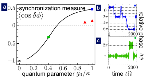
The probability density of the relative phase is either mostly flat (no synchronization) or, as shown in Fig. 3, centered predominantly around or , or it may have two peaks, according to the synchronization regime. In the following, we aim to compress the information contained in the phase distribution into one quantity and calculate the normalized correlator . Its real value, , distinguishes the three different synchronization regimes: (i) for -synchronization, (ii) for -synchronization, (iii) intermediate values of for mixed synchronization. However, this measure has its limitations: When is more or less evenly distributed (no synchronization) , this cannot be distinguished from a mixed synchronization situation where almost equal time is spent in the - and -synchronized states. Furthermore, even in the absence of synchronization (and even in the noiseless case) the phase may spend an increased amount of time around certain values. This leads to a finite value of , and similarly would also show up in the phase distribution. A solution to this problem is to simultaneously look at a part of the corresponding trajectory, where synchronization can easily be distinguished from an unsynchronized state. Instead, one could start to use more complicated correlators, e.g. . This correlator allows to distinguish unsynchronized states from synchronized states, but an additional measure is needed to distinguish - from -synchronization. Note that the imaginary part of the above defined correlator, , can be used as well. However, in the special case of identical optomechanical systems due to the symmetry of the system.
In Fig. 4(a) we show how varies as a function of the quantum parameter . We chose parameters that lead to a mixed synchronization regime for larger values of . In the deep quantum regime ( the probability to find the system in the -synchronized state is larger than the probability to find the phase around , such that . Going towards smaller values of , the ratio increases, such that eventually . Finally, we should reach the classical (noiseless) limit, when . It turns out that, for the parameters adopted here, the classical solution always ends up in the -synchronized state, independent of initial conditions. This implies that there is only one minimum in the effective potential. We conclude that the system has turned from a mixed synchronization regime into a purely -synchronized regime as the quantum parameter was reduced. This cannot be understood in the simple picture of a noise-independent phase potential. We will discuss this kind of behaviour in more detail later on (Sec. VII.3).
Note that the calculations for Fig. 4 have been performed using Langevin equations; although in the deep quantum regime, two data points were also acquired with quantum jump trajectories (red triangles). They are shifted as compared to the Langevin results, but show the same trend. We expect that the difference between the Langevin and quantum jump results decreases for smaller quantum parameters , as it is the case for a single optomechanical system Ludwig et al. (2008). Since smaller require a significantly larger Hilbert space for the quantum jump simulations, we cannot compute this for our coupled system. For large quantum parameter , qualitative differences between the full quantum model and the Langevin equations have been already observed in Ref. Ludwig et al. (2008) as well. Especially a shift of the detuning was reported, that could be determined numerically also for our system. Taking this detuning shift into account would improve the agreement of our results, although differences remain. Here, we show the uncorrected outcomes of both approaches.
VII.2 Residence Times in the Mixed Synchronization Regime
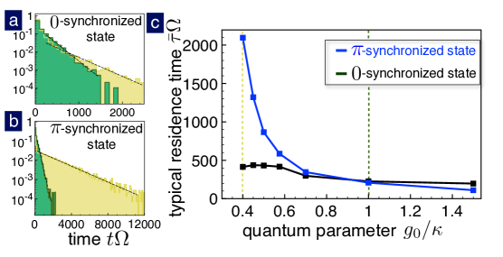
The measure quantifies the fraction of total time spent in -synchronized parts as compared to -synchronized parts. However, it does not provide any information about the rate of transitions between the two synchronization states. Based on the effective potential picture, one might expect the transition rates to be determined by the barrier height and the noise strength. In particular, for larger effective noise strengths , we expect more frequent transitions. This behaviour is qualitatively visible in Fig. 4(b) and (c). However, as concluded in the previous section, the potential picture is not sufficient to explain all observations. Thus, we now turn to a quantitative analysis and discuss how the transition rates between - and -synchronized states (i.e. the typical residence times ) change during the classical-to-quantum crossover. We extract the fluctuating residence times from the phase trajectories and obtain their distribution. The results are shown in Fig. 5(a) and (b) for the - and -synchronized states, for two different quantum parameters . In all cases the probability densities decay exponentially with time, , and the average residence time is obtained from a fit to the distribution. The extracted average residence times and for the two states are shown in Fig. 5(c) as a function of the quantum parameter. Note that the ratio of residence times equals the ratio of probabilities, . Nevertheless, the dependence of the times on reveals new information.
We have chosen parameters such that at both -synchronized and -synchronized parts have almost equal average residence times. This corresponds to and . Furthermore, in the classical limit the system is -synchronized only. When the classical limit is approached, we find that both and increase. As expected, increases much faster than and eventually diverges for , as the system gets trapped forever in the -state. In contrast, increases first when decreasing , but then saturates at a finite level. Such a behaviour is unexpected based on the simple phase potential picture, where a fixed potential would imply diverging residence times for both states in the noiseless limit. The behaviour observed here hinges on the fact that the synchronization regime switches from “mixed” to “” as one reduces the quantum parameter (i.e. reduces the quantum noise). The observations would change significantly for different parameters, where the system always stays in the mixed regime, for any value . Then, one expects the simple picture of a fixed phase potential to be approximately correct and both residence times to diverge as the noise is becoming weaker.
VII.3 Noise-induced Synchronization Bistability
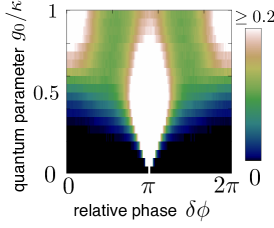
In the previous sections we have explained that some basic features of the classical-to-quantum crossover, like the increase of the residence times with decreasing quantum parameter, can be understood as effects of a decreasing quantum noise strength. The decrease of noise strength leads to less frequent transitions across an energy barrier in the effective potential. However, we made also less easily explained observations: (i) the reverse in the order of and as is being reduced, (ii) the saturation of at low noise levels, (iii) the disappearance of stable -synchronization (for the applied parameters) in the classical limit . Whereas (i) and (ii) could originate from more complicated potential shapes with a combination of broad and narrow minima, (iii) suggests that the effective potential itself changes when the quantum parameter is varied. In Fig. 6 we show how the distribution of evolves as a function of . For very small values of , there is only a single peak close to , in accordance with the single stable solution of the classical limit. While increasing the quantum parameter, this peak is first broadened. The increasing quantum noise strength allows the system to explore more of the effective potential around the minimum. A significant accumulation close to appears only for rather large quantum parameters, signaling the appearance of a second stable solution, i.e. a second minimum in the effective potential at .
In addition to the above described appearance of a second stable solution, there are also parameter regions where already in the classical regime the effective potential has minima at both and (classical bistable synchronization). In this case quantum noise naturally drives transitions between the two synchronization states as soon as it is added to the description of the system. The number of observed transitions then naturally depends on both the noise strength as well as the potential shape.
VIII Overview of synchronization regimes
In the previous sections we have shown examples of the different synchronization regimes in the presence of quantum noise and studied the properties of mixed synchronization in more detail. In the following, we map out the different synchronization regimes as a function of the mechanical coupling and the quantum parameter . Furthermore, we also discuss the case of detuned mechanical oscillators.
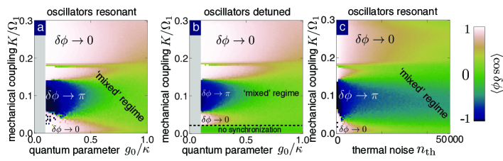
Figure 7(a) shows the synchronization measure for resonant oscillators. We have indicated the synchronization regimes (which are not sharply delineated). For the applied parameters, we find -synchronization for large mechanical coupling in both the quantum and classical regime. In the classical, noiseless limits , indicating less fluctuations around the synchronization state. In contrast, at smaller mechanical coupling, we find more complicated behaviour: there is mixed synchronization for , while the classical limit selects either or synchronization, depending on the mechanical coupling . The “pixelated” region in Fig. 7(a) indicates that the system is multistable even in the classical limit. There, the residence times have become so large that the system is stuck in a random synchronization state depending on initial conditions and the transient behaviour. Notably, the closer the system is to a border of synchronization regimes in the classical limit (this can be seen in Fig. 7(a) for small when is varied), the smaller the noise strength () that is needed to lead to mixed synchronization. As an example, in the ”middle” of the classically -synchronized regime (at about ) similar mixed synchronization as compared to the system close to the regime border () appears only for larger values of the quantum parameter. An exception is of course the classically bistable regime, where mixed synchronization appears naturally as soon as there is noise. An interesting feature appears close to , where the measure shows a sharp dip in the middle of a -synchronized region. We suspect a non-linear resonance, since the oscillator trajectory is no longer simply sinusoidal and period-doubling is observed. At the same time, the oscillation amplitude increases. For larger values of the mechanical coupling , the trajectories are simply sinusoidal again, with the same frequency as for coupling strengths below the feature.
Up to now, we have studied the ideal case of identical mechanical oscillators. We now turn to the case where the mechanical oscillators have slightly different resonance frequencies, i.e. . This is a typical situation in experiments, since fabrication inaccuracies lead to deviations between two systems. Figure 7(b) shows how affects synchronization. A finite corresponds to a tilted effective potential in the classical, noiseless limit, where a finite threshold for synchronization appears Heinrich et al. (2011). This classical threshold is indicated in Fig. 7(b) with a dashed line. Similar behaviour is visible for quantum parameters . However, for large it is not possible to determine the onset of synchronization, because the measure cannot distinguish between no synchronization and mixed synchronization. Instead, we now also have to analyze the trajectories in more detail, which reveal mixed synchronization for sufficiently large mechanical coupling. A significant deviation from the classical threshold cannot be observed at the given resolution. We expect the threshold to slightly increase for larger quantum parameter . At the same time, however, the threshold is also smeared out due to quantum noise.
Here, we have chosen to show the dependence of the synchronization regimes on the mechanical coupling strength and the quantum parameter . Note that other parameters influence the synchronization type as well. In Fig. 2 we have already seen that the laser driving strength and the detuning influence the classical synchronization regimes. Also the mechanical damping can affect the observed synchronization, cf. Fig. 3b and c. However, first of all it already influences the limit cycles of individual optomechanical systems by modifying the threshold to self-sustained oscillations. In addition, has an influence on the mechanical noise strength. Note that, when changing these parameters, care has to be taken to remain on a stable limit cycle for each optomechanical system.
IX Thermal noise
So far, we assumed zero temperature environments for both the optical and the mechanical mode. In this section we investigate the effects of thermal mechanical noise on synchronization.
For our study we use the Langevin equations (5) with modified mechanical noise correlators to account for the coupling of the mechanical oscillators to a finite temperature bath, , where denotes the thermal occupancy of the bath. Hence, both quantum and thermal noise are included. For optical frequencies in the visible spectrum the effective thermal occupation of the optical bath is very small. Thus, the assumption of an optical bath at zero temperature is valid and the optical input noise terms are not modified.
In Fig. 7(c) we show an overview of the synchronization regimes as a function of thermal noise . Here, we chose a comparatively small quantum parameter in order to observe mainly effects due to thermal noise. For small the results are similar to Fig. 7(a) at small . In both cases the influence of the quantum or thermal noise is still weak. For increasing thermal noise strength , we find qualitatively the same behaviour as for increasing quantum noise. However, quantitative differences appear with increasing : Even though a mixed synchronization regime can develop for both quantum and thermal noise, the evolution of the relative weight of both synchronization states is different.
In the following, we want to estimate the critical thermal noise strength at which thermal and quantum noise should have a comparable effect. At lower temperatures, quantum noise will dominate. The main source of quantum fluctuations is the laser shot noise (for the parameters explored here). Thus, we estimate the effect of optical quantum fluctuations on the mechanical oscillator, with the (symmetrized) shot-noise spectrum evaluated at the mechanical resonance frequency Marquardt et al. (2007); Aspelmeyer et al. (2014),
| (7) |
We expect similar effects from quantum and thermal noise if the shot-noise spectrum at the mechanical resonance frequency becomes equal to the thermal force spectrum, . The thermal noise spectrum at temperatures is
| (8) |
where is the temperature of the thermal mechanical bath. Setting and equal, we find (in the resolved sideband regime at ):
| (9) |
where we used the optomechanical cooperativity Aspelmeyer et al. (2014)
| (10) |
This approach suggests that observing quantum noise phenomena does not necessarily require a large and very low temperatures. Instead, if the cooperativity is sufficiently large (comparable to values that enable ground-state cooling, ), quantum noise should dominate the behaviour of the system even in the presence of thermal noise.
However, depending on parameters, we find large deviations from this simple expectation. In these cases, the real shot noise spectrum is no longer well described by the weak-coupling expression of given above, and the actual noise strength may have a much larger value. Consequently, the transition between behaviour dominated by quantum noise vs. that dominated by thermal noise takes place at much larger values of than those predicted by Eq. (9). In other words, it should be even easier to observe quantum noise in optomechanical synchronization than the naive ansatz would lead one to expect.
Here, we don’t observe that quantum noise can be exactly mapped to thermal noise. This is already evident in the rescaled Langevin equations (6). Physically, the thermal force spectrum acting on the mechanical oscillator is flat in frequency, whereas the optical shot-noise spectrum is frequency dependent and is also modified by the dynamics of the system.
X Conclusions
We have investigated the effects of quantum and thermal noise on two coupled optomechanical limit-cycle oscillators. One usually expects that noise prevents strict synchronization, i.e. exact phase locking and a sharp transition to synchronization. Here we have shown that fluctuations additionally drive transitions between - and -synchronization, i.e. the two synchronization states that can appear in the absence of noise. We have discussed the residence times of these states and observed a smooth crossover between different synchronization regimes. Finally, we have compared the effects of quantum and thermal noise. We have argued that it should be possible to experimentally reach the regime where quantum noise dominates. This should happen when the optomechanical cooperativity is large enough for ground state cooling.
For further investigations it would be useful to identify a measure that can genuinely distinguish between an unsynchronized regime and -, - and mixed synchronization. Finally, it will be very interesting to extend the insights obtained here to large optomechanical arrays.
Acknowledgements.
This work was supported by the ITN cQOM as well as ERC OPTOMECH. We thank Steven Habraken and Roland Lauter for discussions and Stefan Walter for his critical reading of the manuscript.References
- Aspelmeyer et al. (2014) M. Aspelmeyer, T. J. Kippenberg, and F. Marquardt, Rev. Mod. Phys. 86, 1391 (2014).
- Hill et al. (2012) J. T. Hill, A. H. Safavi-Naeini, J. Chan, and O. Painter, Nat. Commun. 3, 1196 (2012).
- Dong et al. (2012) C. Dong, V. Fiore, M. C. Kuzyk, and H. Wang, Science 338, 1609 (2012).
- Grudinin et al. (2010) I. S. Grudinin, H. Lee, O. Painter, and K. J. Vahala, Phys. Rev. Lett. 104, 083901 (2010).
- Bahl et al. (2012) G. Bahl, M. Tomes, F. Marquardt, and T. Carmon, Nat. Phys. 8, 203 (2012).
- Wang and Clerk (2012) Y.-D. Wang and A. A. Clerk, Phys. Rev. Lett. 108, 153603 (2012).
- Woolley and Clerk (2014) M. J. Woolley and A. A. Clerk, Phys. Rev. A 89, 063805 (2014).
- Woolley and Clerk (2013) M. J. Woolley and A. A. Clerk, Phys. Rev. A 87, 063846 (2013).
- Paternostro et al. (2007) M. Paternostro, D. Vitali, S. Gigan, M. S. Kim, C. Brukner, J. Eisert, and M. Aspelmeyer, Phys. Rev. Lett. 99, 250401 (2007).
- Deng et al. (2014) Z. J. Deng, S. J. M. Habraken, and F. Marquardt, arXiv:1406.7815 (2014).
- Wang et al. (2015) Y.-D. Wang, S. Chesi, and A. A. Clerk, Phys. Rev. A 91, 013807 (2015).
- Heinrich et al. (2010) G. Heinrich, J. G. E. Harris, and F. Marquardt, Phys. Rev. A 81, 011801 (2010).
- Wu et al. (2013) H. Wu, G. Heinrich, and F. Marquardt, New J. Phys. 15, 123022 (2013).
- Zhang et al. (2012) M. Zhang, G. S. Wiederhecker, S. Manipatruni, A. Barnard, P. McEuen, and M. Lipson, Phys. Rev. Lett. 109, 233906 (2012).
- Maldovan and Thomas (2006) M. Maldovan and E. L. Thomas, Appl. Phys. Lett. 88, 251907 (2006).
- Eichenfield et al. (2009) M. Eichenfield, J. Chan, R. M. Camacho, K. J. Vahala, and O. Painter, Nature 462, 78 (2009).
- Safavi-Naeini et al. (2010) A. H. Safavi-Naeini, T. P. M. Alegre, M. Winger, and O. Painter, Appl. Phys. Lett. 97, 181106 (2010).
- Gavartin et al. (2011) E. Gavartin, R. Braive, I. Sagnes, O. Arcizet, A. Beveratos, T. J. Kippenberg, and I. Robert-Philip, Phys. Rev. Lett. 106, 203902 (2011).
- Laude et al. (2011) V. Laude, J.-C. Beugnot, S. Benchabane, Y. Pennec, B. Djafari-Rouhani, N. Papanikolaou, J. M. Escalante, and A. Martinez, Opt. Express 19, 9690 (2011).
- Safavi-Naeini et al. (2014) A. H. Safavi-Naeini, J. T. Hill, S. Meenehan, J. Chan, S. Gröblacher, and O. Painter, Phys. Rev. Lett. 112, 153603 (2014).
- Chang et al. (2011) D. E. Chang, A. H. Safavi-Naeini, M. Hafezi, and O. Painter, New J. Phys. 13, 023003 (2011).
- Schmidt et al. (2015a) M. Schmidt, V. Peano, and F. Marquardt, New J. Phys. 17, 023025 (2015a).
- Tomadin et al. (2012) A. Tomadin, S. Diehl, M. D. Lukin, P. Rabl, and P. Zoller, Phys. Rev. A 86, 033821 (2012).
- Schmidt et al. (2015b) M. Schmidt, S. Keßler, V. Peano, O. Painter, and F. Marquardt, Optica 2, 635–641 (2015).
- Xuereb et al. (2015) A. Xuereb, A. Imparato, and A. Dantan, New J. Phys. 17, 055013 (2015).
- Peano et al. (2014) V. Peano, C. Brendel, M. Schmidt, and F. Marquardt, Phys. Rev. X 5, 031011 (2015).
- Bhattacharya and Meystre (2008) M. Bhattacharya and P. Meystre, Phys. Rev. A 78, 041801 (2008).
- Xuereb et al. (2012) A. Xuereb, C. Genes, and A. Dantan, Phys. Rev. Lett. 109, 223601 (2012).
- Xuereb et al. (2013) A. Xuereb, C. Genes, and A. Dantan, Phys. Rev. A 88, 053803 (2013).
- Xuereb et al. (2014) A. Xuereb, C. Genes, G. Pupillo, M. Paternostro, and A. Dantan, Phys. Rev. Lett. 112, 133604 (2014).
- Heinrich et al. (2011) G. Heinrich, M. Ludwig, J. Qian, B. Kubala, and F. Marquardt, Phys. Rev. Lett. 107, 043603 (2011).
- Kurths et al. (2001) J. Kurths, A. Pikovsky, and M. Rosenblum, Synchronization: A Universal Concept in Nonlinear Sciences (Cambridge Universitz Press, 2001).
- Giorgi et al. (2012) G. L. Giorgi, F. Galve, G. Manzano, P. Colet, and R. Zambrini, Phys. Rev. A 85, 052101 (2012).
- Höhberger and Karrai (2004) C. Höhberger and K. Karrai, Nanotechnology 2004, Proceedings of the 4th IEEE conference on nanotechnology, 419 (2004).
- Kippenberg et al. (2005) T. J. Kippenberg, H. Rokhsari, T. Carmon, A. Scherer, and K. J. Vahala, Phys. Rev. Lett. 95, 033901 (2005).
- Marquardt et al. (2006) F. Marquardt, J. G. E. Harris, and S. M. Girvin, Phys. Rev. Lett. 96, 103901 (2006).
- Metzger et al. (2008) C. Metzger, M. Ludwig, C. Neuenhahn, A. Ortlieb, I. Favero, K. Karrai, and F. Marquardt, Phys. Rev. Lett. 101, 133903 (2008).
- Ludwig et al. (2008) M. Ludwig, B. Kubala, and F. Marquardt, New J. Phys. 10, 095013 (2008).
- Qian et al. (2012) J. Qian, A. Clerk, K. Hammerer, and F. Marquardt, Phys. Rev. Lett. 109, 253601 (2012).
- Lörch et al. (2014) N. Lörch, J. Qian, A. Clerk, F. Marquardt, and K. Hammerer, Phys. Rev. X 4, 011015 (2014).
- Holmes et al. (2012) C. A. Holmes, C. P. Meaney, and G. J. Milburn, Phys. Rev. E 85, 066203 (2012).
- Lauter et al. (2015) R. Lauter, C. Brendel, S. J. M. Habraken, and F. Marquardt, Phys. Rev. E 92, 012902 (2015).
- Ludwig and Marquardt (2013) M. Ludwig and F. Marquardt, Phys. Rev. Lett. 111, 073602 (2013).
- Walter et al. (2014a) S. Walter, A. Nunnenkamp, and C. Bruder, Phys. Rev. Lett. 112, 094102 (2014a).
- Walter et al. (2014b) S. Walter, A. Nunnenkamp, and C. Bruder, Annalen der Physik 527, 131 (2014b).
- Hermoso de Mendoza et al. (2014) I. Hermoso de Mendoza, L. A. Pachón, J. Gómez-Gardeñes, and D. Zueco, Phys. Rev. E 90, 052904 (2014).
- Lee and Sadeghpour (2013) T. E. Lee and H. R. Sadeghpour, Phys. Rev. Lett. 111, 234101 (2013).
- Lee et al. (2014) T. E. Lee, C.-K. Chan, and S. Wang, Phys. Rev. E 89, 022913 (2014).
- Hush et al. (2015) M. R. Hush, W. Li, S. Genway, I. Lesanovsky, and A. D. Armour, Phys. Rev. A 91, 061401 (2015).
- Xu et al. (2014) M. Xu, D. A. Tieri, E. C. Fine, J. K. Thompson, and M. J. Holland, Phys. Rev. Lett. 113, 154101 (2014).
- Zhirov and Shepelyansky (2009) O. V. Zhirov and D. L. Shepelyansky, Phys. Rev. B 80, 014519 (2009).
- Savel’ev et al. (2012) S. E. Savel’ev, Z. Washington, A. M. Zagoskin, and M. J. Everitt, Phys. Rev. A 86, 065803 (2012).
- Giorgi et al. (2013) G. L. Giorgi, F. Plastina, G. Francica, and R. Zambrini, Phys. Rev. A 88, 042115 (2013).
- Hriscu and Nazarov (2013) A. M. Hriscu and Y. V. Nazarov, Phys. Rev. Lett. 110, 097002 (2013).
- Lee et al. (2013) T. E. Lee, and M. C. Cross, Phys. Rev. A 88, 013834 (2013).
- Mari et al. (2013) A. Mari, A. Farace, N. Didier, V. Giovannetti, and R. Fazio, Phys. Rev. Lett. 111, 103605 (2013).
- Ameri et al. (2015) V. Ameri, M. Eghbali-Arani, A. Mari, A. Farace, F. Kheirandish, V. Giovannetti, and R. Fazio, Phys. Rev. A 91, 012301 (2015).
- Bagheri et al. (2013) M. Bagheri, M. Poot, L. Fan, F. Marquardt, and H. X. Tang, Phys. Rev. Lett. 111, 213902 (2013).
- Matheny et al. (2014) M. H. Matheny, M. Grau, L. G. Villanueva, R. B. Karabalin, M. C. Cross, and M. L. Roukes, Phys. Rev. Lett. 112, 014101 (2014).
- Zhang et al. (2015) M. Zhang, S. Shah, J. Cardenas, and M. Lipson, Phys. Rev. Lett. 115, 163902 (2015).
- Huygens (1673) C. Huygens, Horologium Oscillatorium (Paris: Apud F. Muguet, 1673); English translation: (Ames: Iowa State University Press, 1986).
- Buczek et al. (1972) C. J. Buczek, and R. J. Freiberg, IEEE J. Quantum Electron. 8, 641 (1972).
- Cuomo et al. (1993) K. M. Cuomo, and A. V. Oppenheim, Phys. Rev. Lett. 71, 65 (1993).
- Rosenblum et al. (2003) M. Rosenblum, and A. Pikovsky, Contemp. Phys. 44, 401 (2003).
- Dörfler et al. (2014) F. Dörfler, and F. Bullo, Automatica 50, 1539 (2014).
- Samoilov et al. (2004) M. Samoilov, S. Plyasunov, and A. P. Arkin, PNAS 102, 2310 (2004).
- Biancalani et al. (2014) T. Biancalani, L. Dyson, and A. J. McKane, Phys. Rev. Lett. 99, 038101 (2014).
- Houchmandzadeh et al. (2015) B. Houchmandzadeh, and M. Vallade, Phys. Rev. E 91, 022115 (2015).
- Dykman et al. (1988) M. I. Dykman, and V. N. Smelyanskiy, Zh. Eksp. Teor. Fiz 94, 61 (1988).
- Peano et al. (2006) V. Peano, and M. Thorwart, Chem. Phys. 322, 135 (2006).
- Ghobadi et al. (2011) R. Ghobadi, A. R. Bahrampour, and C. Simon, Phys. Rev. A 84, 033846 (2011).
- Fichthorn et al. (1989) K. Fichthorn, E. Gulari, and R. Ziff, Phys. Rev. Lett. 63, 1527 (1989).
- Kim et al. (1996) S. Kim, S. H. Park, and C. S. Ryu, Phys. Rev. Lett. 78, 1616 (1996).
- Residori et al. (2001) S. Residori, R. Berthet, B. Roman, and S. Fauve, Phys. Rev. Lett. 88, 024502 (2014).
- Kuramoto (1975) Y. Kuramoto, in International Symposium on Mathematical Problems in Theoretical Physics, Lecture Notes in Physics, Vol. 39, edited by H. Araki (Springer Berlin Heidelberg, 1975) pp. 420–422.
- Acebrón et al. (2005) J. A. Acebrón, L. L. Bonilla, C. J. Pérez Vicente, F. Ritort, and R. Spigler, Rev. Mod. Phys. 77, 137 (2005).
- Mølmer et al. (1993) K. Mølmer, Y. Castin, and J. Dalibard, JOSA B 10, 524-538 (1993).
- Plenio and Knight (1998) M. B. Plenio and P. L. Knight, Rev. Mod. Phys. 70, 101 (1998).
- Ludwig et al. (2012) M. Ludwig, A. H. Safavi-Naeini, O. Painter, and F. Marquardt, Phys. Rev. Lett. 109, 063601 (2012).
- Kronwald et al. (2013) A. Kronwald, M. Ludwig, and F. Marquardt, Phys. Rev. A 87, 013847 (2013).
- Akram et al. (2013) U. Akram, W. P. Bowen, and G. J. Milburn, New J. Phys. 15, 093007 (2013).
- Mirza and van Enk (2014) I. M. Mirza and S. J. van Enk, Phys. Rev. A 90, 043831 (2014).
- Cohen et al. (2015) J. D. Cohen, S. M. Meenehan, G. S. MacCabe, S. Gröblacher, A. H. Safavi-Naeini, F. Marsili, M. D. Shaw, and O. Painter, Nature 520, 522 (2015).
- Ueda et al. (1990) M. Ueda, N. Imoto, and T. Ogawa, Phys. Rev. A 41, 3891 (1990).
- Chan et al. (2012) J. Chan, A. H. Safavi-Naeini, J. T. Hill, S. Meenehan, and O. Painter, Appl. Phys. Lett. 101, 081115 (2012).
- Teufel et al. (2011) J. D. Teufel, T. Donner, D. Li, J. W. Harlow, M. S. Allman, K. Cicak, A. J. Sirois, J. D. Whittaker, K. W. Lehnert, and R. W. Simmonds, Nature 475, 359 (2011).
- Murch et al. (2008) K. W. Murch, K. L. Moore, S. Gupta, and D. M. Stamper-Kurn, Nat. Phys. 4, 561 (2008).
- Walls and Milburn (2008) D. Walls and G. J. Milburn, Quantum Optics (Springer-Verlag Berlin Heidelberg, 2008).
- Marquardt et al. (2007) F. Marquardt, J. P. Chen, A. A. Clerk, and S. M. Girvin, Phys. Rev. Lett. 99, 093902 (2007).