Empirical central limit theorem for cluster functionals without mixing.

Abstract

We prove central limit theorems (CLT) for empirical processes of extreme values cluster functionals as in Drees and Rootzén (2010). We use coupling properties enlightened for Dedecker & Prieur’s $\tau-$dependence coefficients in order to improve the conditions of dependence and continue to obtain these CLT. The assumptions are precisely set for particular processes and cluster functionals of interest. The number of excesses provides a complete example of a cluster functional for a simple non-mixing model (AR(1)-process) for which ours results are definitely needed. We also give the expression explicit the covariance structure of limit Gaussian process.

Also we include in this paper some results of Drees (2011) for the extremal index and some simulations for this index to demonstrate the accuracy of this technique.

Keywords and phrases: Extremes, clustering of extremes, cluster functional of extremes, extremal index, uniform central limit theorem, $\tau$-weak dependence, tail empirical process.

1.   Introduction

Drees $\&$ Rootzén, [2010]’s scheme prove limit theorems for empirical process of cluster functionals (EPCF). In statistics, Gómez, [2015] proves a CLT in finite dimensional convergence (fidis) under weaker conditions, and considers an example for which a functional CLT is not necessary.

We extend the result under $\tau$-weak dependence. The classical example of a non-mixing autoregressive model demonstrates the importance of this functional extension. Moreover the estimation of the extremal index provides us with a suitable example of application of the functional CLT.

For a real-valued random process $(X_{i})_{i\in\mathbb{N}}$, a typical example of a EPCF is the tail empirical process:

$$T_{n}(x)=\dfrac{1}{\sqrt{nv_{n}}}\sum_{i=1}^{n}\big{(}\mathbb{1}\{X_{i}>a_{n}x+u_{n}\}-\mathbb{P}(X_{1}>a_{n}x+u_{n})\big{)},\qquad x\ 0,$$ (1)

where $v_{n}=\mathbb{P}\{X_{n,1}\ 0\}$ is decreasing to zero, $(u_{n})_{n\in\mathbb{N}}$ is a non-decreasing sequence of thresholds and $(a_{n})_{n\in\mathbb{N}}$ is a sequence of positive constants. This process has beed considered by Drees and Rootzén under suitable dependence conditions (in particular under $\alpha$ and $\beta$-mixing conditions), where they prove its uniform convergence to a Gaussian process $T$ under additional conditions. For example, they prove the convergence of this tail empirical process for the cases of $k$-dependent sequences or stable AR(1)-processes [Rootzén,, 1995], ARCH(1)-processes [Drees,, 2002, 2003] and some applications for solutions of stochastic difference equations [Drees,, 2000, 2002, 2003]. Finally, they use the cluster functionals setting in [Yun,, 2000] and [Segers,, 2003] to generalize such empirical processes under $\beta$-mixing in [Drees $\&$ Rootzén,, 2010].

Unfortunately, the mixing processes family is very restrictive. This can be noted with the following AR(1)-process, solution of the recursion:

$$X_{k}=\dfrac{1}{b}\big{(}X_{k-1}+\xi_{k}\big{)},\quad k\in\mathbb{Z},$$ (2)

where $b\ 2$ is an integer and $(\xi_{k})_{k\in\mathbb{N}}$ are independent and uniformly distributed random variables on the set $U(b):=\{0,1,\ldots,b-1\}$ which is not even $\alpha-$mixing, as this is shown in [Andrews,, 1984] for $b=2$ and in [Ango Nze $\&$ Doukhan,, 2004] for $b>2$. Thus, the results in [Drees $\&$ Rootzén,, 2010] can not be used here!. However, such process (2) is $\tau$-weakly dependent as is shown in [Dedecker $\&$ Prieur, 2004a, ]. The same situation happens in a general way for the causal Bernoulli shifts, Markovian models, etc. This is thus useful to improve on the CLT for empirical processes of extreme cluster functionals proposed by Drees $\&$ Rootzén, [2010] for more general classes of weakly dependent processes.

In order to do this, we use of the coupling results of Dedecker $\&$ Prieur, 2004a ; Dedecker $\&$ Prieur, [2005] under $\tau$-dependence assumptions to use Van Der Vaart $\&$ Wellner, [1996]’s results of tightness and asymptotic equicontinuity (under independence) together with the fidis convergence of the EPCF.

This paper is organized as follows. In Section 2, we recall basic definitions and notations: cluster functionals, the triangular arrays (or normalized random variables excesses) and examples. Then, we give the definition of cluster functionals empirical processes and close the section with a simple version of the CLT of those empirical processes. In Section 3 we begin with the fidis convergence of the EPCF, followed by the conditions to obtain asymptotic tightness and asymptotic equicontinuity of thoses processes to obtain uniform convergence. We close this section with an application: block estimator of the extremal index. In Section 4 we develop a example similar to (1) for the multidimensional case for the case of the AR(1)-inputs (2). Also a simulation study for the extremal index to demonstrate the accuracy of this technique. The $\tau$-weak dependence with some examples and the proofs are reported in Appendix.

2.   Basic definitions and notations

To define the empirical processes of cluster functionals it is necessary to consider two important ingredients: the cluster functionals and the excesses over high thresholds.

2.1.   Cluster Functionals

Let $(E,\mathcal{E})$ be a measurable subspace of $(\mathbb{R}^{d},\mathcal{B}(\mathbb{R}^{d}))$ for some $d\ 1$ such that $0\in E$. Following the deterministic definition of Drees $\&$ Rootzén, [2010], we consider the set of $E$-valued sequences of finite length, i.e.,

$$E_{\cup}:=\{(x_{1},\ldots,x_{r}):x_{i}\in E\quad\forall i=1,\ldots,r;\quad\forall r\in\mathbb{N}\},$$

equipped with the $\sigma$-field $\mathcal{E}_{\cup}$ induced by Borel-$\sigma$-fields on $E^{r}$, for $r\in\mathbb{N}$. Let $x\in E_{\cup}$, then we can write $x=(x_{1},\ldots,x_{r})$ for some $r\in\mathbb{N}$. The core $x^{c}\in E_{\cup}$ of $x$ is defined by

$$x^{c}:=\left\{\begin{array}[]{cc}(x_{r_{I}},x_{r_{I}+1},\ldots,x_{r_{S}}),&\mbox{ if $x\ 0_{r}$ (the null element in $E^{r}$)}\\ \\ 0,&\mbox{ otherwise}\end{array}\right.$$

where $r_{I}:=\min\{i\in\{1,\ldots,r\}:x_{i}\ 0\}$ (first non-null value of the block $x$) and $r_{S}:=\max\{i\in\{1,\ldots,r\}:x_{i}\ 0\}$ (last non-null value of the block $x$). A cluster functional is a measurable map $f:(E_{\cup},\mathcal{E}_{\cup})\longrightarrow(\mathbb{R},\mathcal{B}(\mathbb{R}))$ such that

$$f(x)=f(x^{c}),\qquad\mbox{ for all }x\in E_{\cup},\ \ \mbox{ and }\ f(0_{r})=0\ (\forall r\ 1).$$ (3)

Under the properties (3), it is easy to build a large amount of examples of cluster functionals. Nevertheless, the typical examples used to build estimators through these cluster functionals are functionals of the type:

$$f(x_{1},\ldots,x_{r})=\sum_{i=1}^{r}\phi(x_{i}),$$ (4)

where $\phi:E\longrightarrow\mathbb{R}$ is a measurable function such that $\phi(0)=0$. Generally speaking, these functions $\phi$ are indicator functions (or functions which are product of another measurable function $H:E\longrightarrow\mathbb{R}$ with an indicator function). Another classic example is the component-wise maximum of a cluster:

$$f(x_{1},\ldots,x_{r})=\max_{1\ i\ r}x_{i},$$ (5)

for $E=[0,\infty)$.

Under the set $E=[0,\infty)$, two particular examples that we shall only mention here with a view to motivating further work, are the following functionals:

• Balanced periods at $u>0$,

  $$f(x_{1},\ldots,x_{r})=\left\{\begin{array}[]{ll}\mathbb{1}{\left\{\sum_{i=1}^{r}(x_{i}-u)\mathbb{1}\{x_{i}>0\}=0\right\}},&\mbox{if $x_{i}>0$ for some $i=1,\ldots,r$}\\ 0,&\mbox{if $x_{i}=0$ for all $i=1,\ldots,r.$}\end{array}\right.$$

• Maximum sum (greater than the level $u>0$) of consecutive excesses,

  $$f(x_{1},\ldots,x_{r})=\max_{1\ p<q\ r}\left(\sum_{y\in H_{p,q}}y\right)\mathbb{1}\left\{\sum_{y\in H_{p,q}}y>u\right\},$$

  with the notation: $H_{p,q}=\{x_{p},x_{p+1},\ldots,x_{q}\}\subseteq\{x_{1},\ldots,x_{r}\}$ such that $y>0$, $\forall y\in H_{p,q}$, where $p,q\in\{1,2,\ldots,r\}$.

2.2.   The excesses and their normalizations

Without going yet into formalities, first let us consider the following examples that motivate the use of the triangular arrays $(X_{n,i})_{1\ i\ n,n\in\mathbb{N}}$ throughout this work.

1.- Let $(X_{i})_{i\in\mathbb{N}}$ be a real-valued stationary random process with marginal cumulative distribution function $F$ and let $(u_{n})_{n\in\mathbb{N}}$ be a non-decreasing sequence of thresholds such that $u_{n}\uparrow x_{F}$, where

$$x_{F}=\sup\{x\in\mathbb{R}:F(x)<1\},\qquad v_{n}=\mathbb{P}\{X_{1}>u_{n}\}\underset{n\to\infty}{\longrightarrow}0.$$

If we want to study the process $X^{\prime}_{n,i}=X_{i}-u_{n}|X_{1}>u_{n}$, first observe that the tail distribution function of $X_{i}$ may be asymptotically degenerated as $n\to\infty$, which means that there exists a point $a\in\mathbb{R}$ such that

$$\overline{P}_{n}(x)=\mathbb{P}\{X_{1}-u_{n}>x|X_{1}>u_{n}\}\underset{n\to\infty}{\longrightarrow}\mathbb{1}\{x\ a\}.$$

However, if $F$ belongs to the domain of attraction of some extreme-value distribution, then by a result in [Pickands,, 1975], there exists $\gamma\in\mathbb{R}$ and a sequence of positive constants $(a_{n})_{n\in\mathbb{N}}$ (depending on the sequence $u_{n}$) such that

$$P_{n}(x)=\mathbb{P}\{X_{n,1}>x|X_{1}>u_{n}\}\underset{n\to\infty}{\longrightarrow}\left\{\begin{array}[]{ll}(1+\gamma x)^{-1/\gamma}_{+},&\mbox{if $\gamma\ 0$}\\ \mathbf{e}^{-x},&\mbox{if $\gamma=0$}\end{array}\right.$$

locally uniform in $(0,\infty)$, where

$$X_{n,i}=\left(\frac{X_{i}-u_{n}}{a_{n}}\right)_{+}:=\max\left\{\frac{X_{i}-u_{n}}{a_{n}},0\right\},\qquad\text{ for }1\leqslant i\leqslant n;$$ (6)

are the normalized excesses of $X_{i}$ over $u_{n}$.

2.- For the multidimensional case we may consider the following example. For $d\ 1$, let $(\mathbf{X}_{i})_{i\in\mathbb{N}}$ be a $\mathbb{R}^{d}$-valued random process such that $\mathbf{X}_{i}=(X^{(1)}_{i},X^{(2)}_{i},\ldots,X^{(d)}_{i})$ admits coordinates with the same marginal distribution, then in this case, a standardization of $\mathbf{X}_{i}$ is:

$$X_{n,i}=\left(\left(\frac{X^{(1)}_{i}-u_{n}}{a_{n}}\right)_{+},\ \left(\frac{X^{(2)}_{i}-u_{n}}{a_{n}}\right)_{+},\ \ldots,\ \left(\frac{X^{(d)}_{i}-u_{n}}{a_{n}}\right)_{+}\right),$$ (7)

where $(u_{n})_{n\in\mathbb{N}}$ and $(a_{n})_{n\in\mathbb{N}}$ are defined as in eqn. (6). Here, $X_{n,i}$ is the vector of normalized excesses over the threshold $u_{n}$ for each coordinate.

Another interesting example is the normalization of $d$ consecutive excesses of real-valued random variables $(X_{i})_{i\in\mathbb{N}}$, i.e.

$$X_{n,i}=\left(\left(\frac{X_{i}-u_{n}}{a_{n}}\right)_{+},\left(\frac{X_{i+1}-u_{n}}{a_{n}}\right)_{+},\ldots,\left(\frac{X_{i+d-1}-u_{n}}{a_{n}}\right)_{+}\right).$$ (8)

This example is given in Section 3 - [Drees $\&$ Rootzén,, 2010]. Observe that this example is a particular case of the example of eqn. (7) which corresponds to $X^{(j)}_{i}=X_{i+j-1}$ for $1\leq j\leq d$.)
Notice that this example brings information on the extremal dependence structure. Some applications of this standardization could be:
(i) $d$ consecutive days of rain are observed in a given city, such that the volume of precipitations may be larger than the volume of water that can be drained (through sewers, soil, rivers, etc.),
(ii) $d$ very large claims are reported to an insurance company in a very small time interval (with respect to typical cases) which this can be a risk with respect to the response capacity of the insurance company, and
(iii) $d$ consecutive days of low temperatures observed in a given city, such that the power consumption (due to heating, etc.) endangers the response capacity of the company in charge of the energy distribution.

In a general way, let $(E,\mathcal{E})$ be a measurable subspace of $(\mathbb{R}^{d},\mathcal{B}(\mathbb{R}^{d}))$ for some $d\ 1$ such that $0\in E$. We denote by $(X_{n,i})_{1\ i\ n}$ as the $E$-valued row-wise stationary standardized random variables, defined on some probability space $(\Omega,\mathcal{A},\mathbb{P})$, which are built from a stationary random process $(X_{i})_{i\in\mathbb{Z}}$, in a way such that the standardization $X_{n,i}$ maps all "non-extreme" values to zero. Additionally, it should satisfy that the sequence of conditional distributions of $X_{n,1}$ given that $X_{n,1}$ belongs of the failure set $S\subseteq E\setminus\{0\}$ (i.e. $P_{n}(\cdot|S):=\mathbb{P}\{X_{n,1}\in\cdot|X_{n,1}\in S\}$), converge weakly to some non-degenerate limit.

2.3.   Empirical Processes of Cluster Functionals

Now, we want to apply cluster functionals to blocks of $E$-valued random variables excesses over a determined thresholds sequence and to define the empirical process indexed by these functionals.

In order to do that, first let us consider a row-wise stationary $E$-valued triangular array $(X_{n,i})_{1\ i\ n,n\in\mathbb{N}}$, defined on some probability space $(\Omega,\mathcal{A},\mathbb{P})$.

Let $Y_{n,j}$ be the $j$-th block of $r_{n}$ consecutive values of the $n$-th row of $(X_{n,i})$. That is, we have $m_{n}:=[n/r_{n}]=\max\{j\in\mathbb{N}:j\ n/r_{n}\}$ blocks

$$Y_{n,j}:=(X_{n,i})_{(j-1)r_{n}+1\ i\ jr_{n}}$$ (9)

of length $r_{n}$, with $1\ j\ m_{n}$. In order to simplify future notations, since $(X_{n,i})_{1\ i\ n}$ is stationary for each $n$, then we can denote by $Y_{n}$ to the "generic block" such that $Y_{n}\overset{\mathcal{D}}{=}Y_{n,1}$.
Let $\mathcal{F}$ be a class of cluster functionals. The "empirical process $Z_{n}$ of cluster functionals” in $\mathcal{F}$, is the process $(Z_{n}(f))_{f\in\mathcal{F}}$ defined by

$$Z_{n}(f):=\frac{1}{\sqrt{nv_{n}}}\sum_{j=1}^{m_{n}}(f(Y_{n,j})-\mathbb{E}f(Y_{n,j})),$$ (10)

where $v_{n}:=\mathbb{P}\{X_{n,1}\in S\}$ and $S$ is the failure set.

In order to begin approaching the convergence in fidis of the EPCF (10), observe that if the blocks $(Y_{n,j})_{1\ j\ m_{n},n\in\mathbb{N}}$ are independents and if we take in account the following essential convergence assumptions:

• $\mathbb{E}\left[\left(f(Y_{n})-\mathbb{E}f(Y_{n})\right)^{2}\mathbb{1}\left\{|f(Y_{n})-\mathbb{E}f(Y_{n})|>\epsilon\sqrt{nv_{n}}\right\}\right]=o(r_{n}v_{n})$,
  for all $\epsilon>0$, and for all $f\in\mathcal{F}$.

• $(r_{n}v_{n})^{-1}\mbox{Cov}\left(f(Y_{n}),g(Y_{n})\right)\longrightarrow c(f,g)$, for all $f,g\in\mathcal{F}$,

with $r_{n}\ll v_{n}^{-1}\ll n$, then the fidis of the empirical process $(Z_{n}(f))_{f\in\mathcal{F}}$ of cluster functionals converge to the fidis of a Gaussian process $(Z(f))_{f\in\mathcal{F}}$ with the covariance function $c$.

Drees $\&$ Rootzén, [2010] have proved CLTs for the process (10). In particular, they have proved CLTs in fidis for this process by using the Bernstein blocks technique together with a $\beta$-mixing coupling condition to boil down convergence to convergence of sums over i.i.d. blocks through Eberlein, [1984]’s technique involving the metric of total variation. Moreover, Drees $\&$ Rootzén, [2010] extend the results to the uniform convergence by adding Van Der Vaart $\&$ Wellner, [1996]’s tightness criteria and asymptotic equicontinuity conditions to the results in fidis that they had obtained.

We aim at extending their CLT’s for the empirical process $(Z_{n}(f))_{f\in\mathcal{F}}$, since the family of mixing processes is still very restrictive. One particular and really simple example of a non-mixing process is the AR(1)-process (2). We derive some results as in [Drees $\&$ Rootzén,, 2010] and some applications as in [Drees,, 2011] under much weaker dependence conditions including eg. this example.
The $\tau-$weak dependence introduced by Dedecker $\&$ Prieur, 2004a holds for the Example in eqn. (2), as well as more generally for Bernoulli shifts processes and Markov chains.

3.   Central limit theorems for cluster functionals

3.1.   Fidis convergence

First we give the convergence in fidis. In this case, the technique used to prove the convergence of the empirical process (10) is also the Bernstein blocks technique. In order to do this, we need to extract from each block $Y_{n,j}$ of length $r_{n}$ a sub-block of length $l_{n}$, in such a way that $l_{n}=o(r_{n})$. Then we use the remaining sub-blocks, separated by $l_{n}$ variables, combined with convenient conditions of $\tau$-dependence to couple independent blocks to the original blocks (originally dependent), and thus obtain the CLTs through classic tools.

For this, it is necessary for the triangular array $(X_{n,i})_{1\ i\ n,n\in\mathbb{N}}$ to satisfy the relation:

• $\tau_{1,n}(l_{n})=o(r_{n}^{-1})$,

such that

• $l_{n}\ll r_{n}\ll v_{n}^{-1}\ll n$ where $l_{n}\longrightarrow\infty$ and $nv_{n}\longrightarrow\infty$ as $n\to\infty$, and

• $\mathbb{E}\left(\|X_{n,1}\||X_{n,1}\ 0\right)<\infty.$

On the other hand, we must not forget the influence of the small blocks extracted with length $l_{n}$ over the empirical process (10). In this case, in order to introduce assumptions over these small blocks, it is necessary to consider the following notations, which we will also use throughout the rest of this paper.

Notation 1

Let $x=(x_{1},x_{2},\ldots,x_{r})$. We will use the notation $x^{[l:k]}$ as follows

$$x^{[l:k]}=\left\{\begin{array}[]{ll}0,&\mbox{if $r<l$},\\ (x_{l},\ldots,x_{k}),&\mbox{if $1\ l\ k\ r$},\\ Y,&\mbox{if $k>r$.}\end{array}\right.$$

and $x^{[k]}:=x^{[1:k]}$. Moreover, if $f\in\mathcal{F}$ is a cluster functional, then we denote

$$\Delta_{n}(f):=f(Y_{n})-f(Y_{n}^{[r_{n}-l_{n}]}),$$ (11)

where $r_{n}$ is the length of the block $Y_{n}$ and $l_{n}$ is such that $l_{n}=o(r_{n})$.

The following assumption guarantees that the extraction of the small blocks does not disturb the result of the convergence in fidis (if that is the case) of the EPCF $(Z_{n}(f))_{f\in\mathcal{F}}$.

• For all $f\in\mathcal{F}$,

  $$\mathbb{E}|\Delta_{n}(f)-\mathbb{E}\Delta_{n}(f)|^{2}\mathbb{1}\left\{|\Delta_{n}(f)-\mathbb{E}\Delta_{n}(f)|\ \sqrt{nv_{n}}\right\}= o(r_{n}v_{n})$$

  $$\mathbb{P}\left\{|\Delta_{n}(f)-\mathbb{E}\Delta_{n}(f)|>\sqrt{nv_{n}}\right\}= o(r_{n}/v_{n}).$$

Theorem 1

Suppose that (B.1)-(B.2), (C.1)-(C.3) and (D.1) hold. Then the fidis of the cluster functionals empirical process $(Z_{n}(f))_{f\in\mathcal{F}}$ converge to the fidis of a centered Gaussian process $(Z(f))_{f\in\mathcal{F}}$ with covariance function $c$ defined in assumption (C.2).

Remark 1

Note that Assumptions (C.1) and (C.3) are difficult to check in general, for that reason, consider the following (more restrictive but easier to verify) alternatives conditions:

• $\mbox{Var}(\Delta_{n}(f))=o(r_{n}v_{n})$ for all $f\in\mathcal{F}$.

• $\mathbb{E}(f(Y_{n}))^{2+\delta}=O(r_{n}v_{n})$ for some $\delta>0$ and for all $f\in\mathcal{F}$.

Lemma 1

The conditions (A.1) and (A.3) implies the conditions (C.1) and (C.3), respectively.

For the proof of this lemma see Lemma 5.2 in [Drees $\&$ Rootzén,, 2010].

Generally, the (C.2) convergence can be easily verified. However, in some situations it could be difficult to give the limit $c$ in an explicit mode. In this sense, it is common to use the "tail chain" associated to the original process $(X_{i})_{i\in\mathbb{N}}$. This terminology was used by Perfekt, [1994], but generalized by Yun, [1998] to make explicit representations of the extremal index of a higher-order stationary Markov chain. Segers, [2003] generalizes this result to stationary sequences with suitable conditions.

We will follow Segers, [2003] rationale to give an explicit representation of the covariance function $c$ through the tail chains. The following proposition (which is a similar result to Segers, [2003]’s Theorems 1 and 3) provide some conditions, sufficient to verify (C.2) and which in some situations are easier to prove. The alternative expression to the covariance function c (defined in (C.2)), is shown below in Corollary 1.

In order to carry this out, it is necessary to consider the following assumption:

• There is a sequence $W=(W_{i})_{i\ 1}$ of $E$-valued random variables such that, for all $k\in\mathbb{N}$, the joint conditional distribution

  $$P_{(X_{n,i},\mathbb{1}\{X_{n,i}=0\})_{1\ i\ k}|X_{n,1}\ 0}$$

  converges weakly to $P_{(W_{i},\mathbb{1}\{W_{i}=0\})}$, and for all $f\in\mathcal{F}$ are a.s. continuous with respect to the distribution of $W^{[k]}=(W_{1},\ldots,W_{k})$ and $W^{[2:k]}=(W_{2},\ldots,W_{k})$ for all $k$, that is,

  $$\mathbb{P}\{W^{[2:k]}\in D_{f,k-1},W_{i}=0,\ \forall i>k\}=\mathbb{P}\{W^{[k]}\in D_{f,k},W_{i}=0,\ \forall i>k\}=0$$

  where we denote by $D_{f,k}$ the set of discontinuities of $f|_{E^{k}}$.

Remark 2

The existence of such sequence $W$ is guaranteed in particular from Theorem 2 in [Segers,, 2003] with $E=\mathbb{R}$ and the normalization (6). There, Segers has shown that if

$$\mathbb{P}_{((X_{n,i})_{1\ i\ k}|X_{1}>u_{n})}\underset{n\to\infty}{\longrightarrow}-\log G_{k},$$

where $G_{k}$ is some $k-$dimensional extreme value distribution for all $k\in\mathbb{N}$, then there exists such "tail chain" $W=(W_{i})_{i\in\mathbb{N}}$ such that

$$P_{((X_{n,i},\mathbb{1}\{X_{n,i}=0\})_{1\ i\ k}|X_{1}>u_{n})}\overset{w}{\underset{{}_{n\to\infty}}{\longrightarrow}}P_{(W_{i},\mathbb{1}\{W_{i}=0\})_{1\ i\ k}},$$ (12)

for all $k\in\mathbb{N}$.

Proposition 1

Suppose that the r.v’s $(X_{n,i})_{1\ i\ n,n\in\mathbb{N}}$ satisfies the following condition:

• There exists $p,q\ 1$ with $p^{-1}+q^{-1}=1$ and $\alpha>0$, such that

  $$\lim_{l\to\infty}\limsup_{n\to\infty}\dfrac{r_{n}\tau_{p,n}(l)}{v_{n}^{1/p+\alpha}}=0\qquad\text{and }\qquad r_{n}v_{n}^{1/q}\underset{n\to\infty}{\longrightarrow}0$$ (13)

Then,

$$\mathbb{E}\left[f(Y_{n})|Y_{n}\ 0\right]=\theta_{n}^{-1}\mathbb{E}\left[f(Y_{n,1})-f(Y_{n,1}^{[2:r_{n}]})|X_{n,1}\ 0\right]+o(1),$$

where $o(1)$ converges to $0$ as $n\to\infty$ uniformly for all bounded cluster functionals $f\in\mathcal{F}$, and

$$\theta_{n}:=\dfrac{\mathbb{P}\{Y_{n}\ 0\}}{r_{n}v_{n}}=\mathbb{P}\{Y_{n,1}^{[2:r_{n}]}=0|X_{n,1}\ 0\}(1+o(1)).$$ (14)

Additionally, if the assumption (C.2’) is satisfied, then:

$$\begin{array}[]{cll}m_{W}&:=&\sup\{i\ 1:W_{i}\ 0\}<\infty,\\ \theta_{n}&\underset{{}_{n\to\infty}}{\longrightarrow}&\theta:=\mathbb{P}\{W_{i}=0,\forall i\ 2\}=\mathbb{P}\{m_{W}=1\}>0,\\ P_{f(Y_{n})|Y_{n}\ 0}&\overset{w}{\underset{{}_{n\to\infty}}{\longrightarrow}}&\dfrac{1}{\theta}\left(\mathbb{P}\{f(W)\in\cdot\}-\mathbb{P}\{f(W^{[2:\infty]})\in\cdot,m_{W}\ 2\}\right).\end{array}$$

Corollary 1

Suppose that

$$\mathcal{F}=\{f|(f(Y_{n})^{2})_{n\in\mathbb{N}}\text{ is uniformly integrable under }P(\cdot)/r_{n}v_{n}\}.$$

Assume that (B.1), (B.2), (C.2’), (C.3) and (D.2) hold. Then the fidis of the cluster functionals empirical process $(Z_{n}(f))_{f\in\mathcal{F}}$ converge to the fidis of a centered Gaussian process $(Z(f))_{f\in\mathcal{F}}$ with covariance function $c$ defined by

$$c(f,g)=\mathbb{E}\left[(fg)(W)-(fg)(W^{[2:\infty]})\right].$$ (15)

There are many cases in which $\|f\|_{\infty}=\sup_{x\in E_{\cup}}|f(x)|<\infty$, for all $f\in\mathcal{F}$. Under this condition, it is clear that the conditions (C.1) and (C.3) are satisfied. Therefore, it is important to note the following corollary.

Corollary 2

Suppose that (B.1), (B.2), (C.2’) and (D.2) are satisfied. Then, if $\|f\|_{\infty}=\sup_{x\in E_{\cup}}|f(x)|<\infty$ for all $f\in\mathcal{F}$, the fidis of the cluster functionals empirical process $(Z_{n}(f))_{f\in\mathcal{F}}$ converges to the fidis of a centered Gaussian process $(Z(f))_{f\in\mathcal{F}}$ with covariance function $c$ defined by (15).

3.2.   Uniform convergence

To prove uniform convergence, we use either asymptotic tightness of $Z_{n}$ in the space $\ell^{\infty}(\mathcal{F})$, or asymptotic equicontinuity conditions, by some results in §  2.11 of Van Der Vaart $\&$ Wellner, [1996]. Those results need independence therefore a argument of coupling for the blocks $(Y_{n,j})_{1\ j\ m_{n},n\in\mathbb{N}}$ is also used here.

3.2.1 Asymptotic tightness

Definition 1

The sequence $(Z_{n})_{n\in\mathbb{N}}$ is asymptotically tight if for every $\epsilon>0$ there exists a compact set $K\in\ell^{\infty}(\mathcal{F})$ such that

$$\limsup_{n\longrightarrow\infty}\mathbb{P}^{*}(Z_{n}\notin K^{\delta})<\epsilon,\quad\text{ for every }\delta>0,$$

where $K^{\delta}=\{f\in\ell^{\infty}(\mathcal{F}):d_{\mathcal{F}}(f,K)<\delta\}$ is the "$\delta-$enlargement" around $K$ and $\mathbb{P}^{*}$ denotes the outer probability.

Definition 2

The bracketing number $N_{[\cdot]}(\epsilon,\mathcal{F},L_{2}^{n})$ is defined as the smallest number $N_{\epsilon}$ such that for each $n\in\mathbb{N}$ there exits a partition $(\mathcal{F}_{n,k}^{\epsilon})_{1\ k\ N_{\epsilon}}$ of $\mathcal{F}$ such that

$$\mathbb{E}^{*}\sup_{f,g\in\mathcal{F}_{n,k}^{\epsilon}}\left(f(Y_{n})-g(Y_{n})\right)^{2}\ \epsilon^{2}r_{n}v_{n},\hskip 14.22636pt\mbox{ for }\quad 1\ k\ N_{\epsilon},$$

where $\mathbb{E}^{*}$ denotes the outer expectation.

In order to use Theorem 2.11.9 in [Van Der Vaart $\&$ Wellner,, 1996] we need:

• The set $\mathcal{F}$ of cluster functionals is such that for each $f\in\mathcal{F}$ the expression $\mathbb{E}f^{2}(Y_{n})$ is finite for all $n\in\mathbb{N}$ and such that the envelope function satisfies:

  $$F(x):=\sup_{f\in\mathcal{F}}|f(x)|<\infty,\qquad\forall x\in E_{\cup}.$$

• $\mathbb{E}^{*}\left(F(Y_{n})\mathbb{1}\{F(Y_{n})>\epsilon\sqrt{nv_{n}}\}\right)=o(r_{n}\sqrt{v_{n}/n})$ for all $\epsilon>0$.

Note that for a sequence of monotonically increasing positive functions $(h_{n}(\delta))_{n\ 1}$ the convergence of $h_{n}(\delta_{n})$ to zero $\forall\delta_{n}\downarrow 0$ is equivalent to

$$\lim_{\delta\downarrow 0}\limsup_{n\longrightarrow\infty}h_{n}(\delta)=0,$$

thus the Assumptions 2 and 3 of Theorem 2.11.9 from [Van Der Vaart $\&$ Wellner,, 1996] are reformulated as follows:

• There exists a semi-metric $\rho$ on $\mathcal{F}$ such that $\mathcal{F}$ is totally bounded with respect to (w.r.t.) $\rho$ and

  $$\lim_{\delta\downarrow 0}\limsup_{n\longrightarrow\infty}\sup_{f,g\in\mathcal{F}:\rho(f,g)<\delta}\dfrac{1}{r_{n}v_{n}}\mathbb{E}\left(f(Y_{n})-g(Y_{n})\right)^{2}=0.$$

• $$\lim_{\delta\downarrow 0}\limsup_{n\longrightarrow\infty}\int_{0}^{\delta}\sqrt{\log N_{[\cdot]}(\epsilon,\mathcal{F},L_{2}^{n})}d\epsilon=0.$$

Theorem 2

Suppose that (B.1), (B.2), (D.1) hold and that (T.1) - (T.4) are satisfied. Then the empirical process $(Z_{n})_{n\in\mathbb{N}}$ is asymptotically tight in $\ell^{\infty}(\mathcal{F})$. Moreover, if the assumptions (C.1)-(C.3) hold, then $Z_{n}$ converges to a centered Gaussian process $Z$ with covariance function $c$ in (C.2).

3.2.2 Asymptotic equicontinuity

Definition 3

The sequence $(Z_{n})_{n\in\mathbb{N}}$ is asymptotically equicontinuous w.r.t. a semi-metric $\rho$ if for any $\epsilon>0$ and $\eta>0$ there exists some $\delta>0$ such that:

$$\limsup_{n\longrightarrow\infty}\mathbb{P}^{*}\left(\sup_{f,g\in\mathcal{F}:\;\rho(f,g)<\delta}|Z_{n}(f)-Z_{n}(g)|>\epsilon\right)<\eta.$$

We use Theorem 2.11.1 in [Van Der Vaart $\&$ Wellner,, 1996] to prove asymptotic equicontinuity. In order to do this, we need to define a semi-metric $\rho_{n}$ on $\mathcal{F}$ as follows. Let $(Y^{*}_{n,j})_{1\ j\ m_{n}}$ be the independent copies of $(Y_{n,j})_{1\ j\ m_{n}}$.
We define $\rho_{n}$ as:

$$\rho_{n}(f,g):=\sqrt{\dfrac{1}{nv_{n}}\sum_{j=1}^{m_{n}}(f(Y_{n,j}^{*})-g(Y_{n,j}^{*}))^{2}}.$$ (16)

Moreover, we denote by $N(\epsilon,\mathcal{F},\rho)$ the "covering number", the minimum number of balls (w.r.t. the semi-metric $\rho$) with radius $\epsilon>0$ necessary to cover $\mathcal{F}$. In this way, we can add to the list of assumptions the following two:

• For $k=1,2$ the map

  $$(Y^{*}_{n,1},\ldots,Y^{*}_{n,[m_{n}/2]})\longmapsto\sup_{f,g\in\mathcal{F}:\rho(f,g)<\delta}\sum_{j=1}^{[m_{n}/2]}e_{j}\left(f(Y_{n,j}^{*})-g(Y_{n,j}^{*})\right)^{k}$$

  is measurable for each $\delta>0$, each vector $(e_{1},\ldots,e_{[m_{n}/2]})\in\{-1,0,1\}^{[m_{n}/2]}$ and each $n\in\mathbb{N}$.

• $$\lim_{\delta\downarrow 0}\limsup_{n\longrightarrow\infty}\mathbb{P}^{*}\left(\int_{0}^{\delta}\sqrt{\log N(\epsilon,\mathcal{F},\rho_{n})}d\epsilon>\eta\right)=0\text{, }\hskip 14.22636pt\forall\eta>0.$$

Theorem 3

Suppose that (B.1), (B.2), (D.1) hold and that (T.1)-(T.3), (T.4’) and (T.5) are satisfied. Then the empirical process $(Z_{n})_{n\in\mathbb{N}}$ is asymptotically equicontinuous. Moreover if the assumptions (C.1)-(C.3) hold, then $Z_{n}$ converges to a centered Gaussian process $Z$ with covariance function $c$ in (C.2).

3.3.   Application: blocks estimator of the extremal index

Let $(X_{i})_{i\in\mathbb{N}}$ be a real stationary time series with distribution function $F$. Now consider the index defined in (14) with the extreme normalization (6) and $u_{n}:=F^{\leftarrow}(1-v_{n}t)$, for all $t\in[0,1]$, i.e.

$$\theta_{n,t}:=\dfrac{\mathbb{P}\{Y_{n}\ 0\}}{r_{n}v_{n}t}=\dfrac{\mathbb{P}\{\max_{1\ i\ r_{n}}X_{i}>u_{n}\}}{r_{n}v_{n}t},\quad\text{ with }t\in(0,1].$$ (17)

Note that if $r_{n}$ satisfies (B.1) condition and if (D.2) holds, then by using Proposition 1, there exists a number (extremal index) $\theta\in(0,1]$ such that

$$\theta_{n,t}\underset{{}_{n\to\infty}}{\longrightarrow}\theta\quad\text{ uniformly for }t\in(0,1].$$ (18)

Given the convergence (18), Drees has suggested in his paper Drees, [2011] to estimate $\theta$ replacing the unknown probability $\mathbb{P}\{\max_{1\ i\ r_{n}}X_{i}>u_{n}\}$ and the unknown expectation $r_{n}v_{n}t=\mathbb{E}\left[\sum_{i=1}^{r_{n}}\mathbb{1}\{X_{i}>u_{n}\}\right]$ by a empirical expression for $\theta_{n,t}$:

$$\widehat{\theta}_{n,t}:=\dfrac{\sum_{j=1}^{m_{n}}\mathbb{1}\{\max_{(j-1)r_{n}<i\ jr_{n}}X_{i}>u_{n}\}}{\sum_{j=1}^{m_{n}}\sum_{i=(j-1)r_{n}+1}^{jr_{n}}\mathbb{1}\{X_{i}>u_{n}\}},$$ (19)

where $m_{n}=[n/r_{n}]$ such that $1\ll r_{n}\ll v_{n}^{-1}\ll n$ but $nv_{n}\longrightarrow\infty$. Thus, such estimator (19) (called blocks estimator of the extremal index) can be expressed in terms of two empirical processes of cluster functionals $(Z_{n}(f_{t}),Z_{n}(g_{t}))_{0\ t\ 1}$ defined in (10). For this, suppose without loss of generality that the random variables $(X_{i})_{1\ i\ n}$ are uniformly distributed on $[0,1]$ (otherwise, just consider the transformation $U_{i}=F(X_{i})$, $1\ i\ n$, where $F$ is the distribution function of $X_{1}$, see Drees, [2011]). Then, with the normalization (6) such that $a_{n}=v_{n}=1-u_{n}$ and the blocks $(Y_{n,j})_{1\ j\ m_{n}}$ defined in (9), we have that

$$\widehat{\theta}_{n,t}=\dfrac{m_{n}^{-1}\sum_{j=1}^{m_{n}}f_{t}(Y_{n,j})}{m_{n}^{-1}\sum_{j=1}^{m_{n}}g_{t}(Y_{n,j})}=\dfrac{\mathbb{E}f_{t}(Y_{n,1})+(nv_{n})^{1/2}m_{n}^{-1}Z_{n}(f_{t})}{\mathbb{E}g_{t}(Y_{n,1})+(nv_{n})^{1/2}m_{n}^{-1}Z_{n}(g_{t})},$$ (20)

where

$$f_{t}(x_{1},\ldots,x_{r}) :=\mathbb{1}\{\max_{1\ i\ r}x_{i}>1-t\}$$ (21)

$$g_{t}(x_{1},\ldots,x_{r}) :=\sum_{i=1}^{r}\mathbb{1}\{x_{i}>1-t\}.$$ (22)

For this particular case, we consider the following assumptions:

• $(r_{n}v_{n})^{-1}\mbox{Cov}(g_{s}(Y_{n}),g_{t}(Y_{n}))\longrightarrow c_{g}(s,t)$, for all $0\ s,t\ 1$.

• $(r_{n}v_{n})^{-1}\mbox{Cov}(f_{s}(Y_{n}),g_{t}(Y_{n}))\longrightarrow c_{fg}(s,t)$, for all $0\ s,t\ 1$.

• For some bounded function $h:(0,1]\longrightarrow\mathbb{R}$ such that $\lim_{t\to 0}h(t)=0$

  $$(r_{n}v_{n})^{-1}\mathbb{E}\left(f_{s}(Y_{n,1})-f_{t}(Y_{n,1})\right)^{2}\ h(t-s),\quad\forall 0\ s<t\ 1,$$

  for all $n$ sufficiently large.

The following are a slight variation of the first two results of Drees, [2011], in the sense that we replace the $\beta$-mixing condition with $\tau$-dependence condition.

Proposition 2

• Suppose that (B.1), (B.2) and (D.1) are satisfied. Then $(Z_{n}(f_{t}))_{0\ t\ 1}$ converges weakly to $Z_{f}:=(\sqrt{\theta}B_{t})_{0\ t\ 1}$, where $B$ denote a standard Brownian motion.

• If additionally (C.2.1) and (T) are satisfied and $r_{n}=o(\sqrt{nv_{n}})$, then the sequence of processes $(Z_{n}(g_{t}))_{0\ t\ 1}$ converges weakly to a centered Gaussian process $(Z_{g}(t))_{0\ t\ 1}$ with covariance function $c_{g}$.

• Under all the hypothesis of (3.1) and (3.2), if moreover (C.2.2) holds, then $(Z_{n}(f_{t}),Z_{n}(g_{t}))_{0\ t\ 1}$ converge weakly to $(Z_{f}(t),Z_{g}(t))_{0\ t\ 1}$ with

  $$\mbox{Cov}(Z_{f}(s),Z_{f}(t)) =\theta(s\land t),$$

  $$\mbox{Cov}(Z_{g}(s),Z_{g}(t)) =c_{g}(s,t),$$

  $$\mbox{Cov}(Z_{f}(s),Z_{g}(t)) =c_{fg}(s,t),\quad 0\ s,t\ 1.$$ (23)

Using the same argument in Remark 2, we can find explicit expressions for the covariance functions $c_{g}$ and $c_{fg}$ as functions of the "tail chains" of $(X_{i})_{i\in\mathbb{N}}$. This is, if for every $k\in\mathbb{N}$ the distribution function of $(X_{1},\ldots,,X_{k})$ belongs to the domain of attraction of an extreme-value distribution, then there exist a sequence $W=(W_{i})_{i\in\mathbb{N}}$ such that (12) hold. In such case:

$$c_{g}(s,t) =s\land t+\sum_{i=1}^{\infty}\left(\mathbb{P}\{W_{1}>1-s,W_{i+1}>1-t\}+\mathbb{P}\{W_{1}>1-t,W_{i+1}>1-s\}\right)$$

$$c_{fg}(s,t) =\left\{\begin{array}[]{ll}\mathbb{P}\{W_{1}>1-t,\max_{j\ 1}W_{j}>1-s\}&\\ +\sum_{i=1}^{\infty}\mathbb{P}\{W_{1}>1-s,W_{i+1}>1-t,\max_{j\ 2}W_{j}\ 1-s\},&s<t,\\ t&s\ t.\end{array}\right.$$ (27)

Corollary 3

Under Proposition 2 - (3.3)’s assumptions,

$$(\sqrt{nv_{n}}t(\widehat{\theta}_{n,t}-\theta_{n,t}))_{0<t\ 1}\overset{w}{\underset{{}_{n\to\infty}}{\longrightarrow}}Z:=Z_{f}-\theta Z_{g},$$ (28)

where $Z$ is a Gaussian process such that $\mathbb{E}Z(t)=0$ and

$$\mbox{Cov}(Z(s),Z(t))=\theta(s\land t-c_{fg}(s,t)-c_{fg}(t,s)+\theta^{2}c_{g}(s,t)).$$ (29)

4.   Examples and Simulations

4.1.   AR(1)-process with the functional "number of excesses over $x$"

We consider the AR(1)-process (2) where $b\ 2$ is an integer, $(\xi_{i})_{i\in\mathbb{N}}$ are i.i.d. and uniformly distributed on the set $U(b):=\{0,1,\ldots,b-1\}$.
It is clear that $X_{0}$ is uniformly distributed on $[0,1]$. Moreover we define the normalized random variables $(X_{n,i})_{1\ i\ n,n\in\mathbb{N}}$ as in eqn. (8) with $a_{n}=v_{n}=1-u_{n}$. We set $(x_{1},\ldots,x_{d})\ (y_{1},\ldots,y_{d})$ if and only if $x_{i}\ y_{i}$, for all $i=1,\ldots,d$ in case $x,y\in[0,1]^{d}$. Then

$$\mathbb{P} \{X_{n,1}>x|X_{n,1}\ 0\}$$

$$= \dfrac{1}{b^{d}\bar{v}_{n}}\sum_{j_{1},\ldots,j_{d}\in U(b)}\left(\max_{i=1,\ldots,d}\left\{1-b^{i}+\sum_{s=1}^{i}b^{s-1}j_{s}+b^{i}v_{n}(1-x_{i})\right\}_{+}\land 1\right)$$

$$\underset{{}_{n\to\infty}}{\longrightarrow} \max_{i=1,\ldots,d}\{b^{i-d}(1-x_{i})\},$$ (30)

where $\bar{v}_{n}:=\mathbb{P}\{X_{n,1}\ 0\}\sim\ v_{n}=\mathbb{P}\{X_{1}>u_{n}\}\underset{{}_{n\to\infty}}{\longrightarrow}0$.

Consider $\mathcal{F}$ the family of cluster functionals:

$$\mathcal{F}=\left\{f_{x},\ {x\in[0,1]^{d}}\right\},\quad\mbox{ with }\quad f_{x}(x_{1},\ldots,x_{r})=\sum_{i=1}^{r}\mathbb{1}\{x_{i}>x\}$$ (31)

For this case, we obtain the covariance function $c$ of (C.2):

$$c(x,y)= \min\left(\max_{k=1,\ldots,d}\{b^{k}(1-x_{k})\},\max_{k=1,\ldots,d}\{b^{k}(1-y_{k})\}\right)$$

$$+\sum_{i=1}^{\infty}H_{b,i}(x,y)+\sum_{i=1}^{\infty}H_{b,i}(y,x),$$ (32)

where, for $i\ d$

$$H_{b,i}(x,y):=\dfrac{1}{b^{i}}\min\left(\max_{k=1\ldots,d}\{b^{k}(1-x_{k})\},\max_{k=1,\ldots,d}\{b^{k+i}(1-y_{k})\}\right)$$ (33)

and for $1\ i<d$,

$$H_{b,i}(x,y)$$

$$:=\dfrac{1}{b^{i}}\min\left(\max_{k=1\ldots,i}\{b^{k}(1-x_{k})\},\max_{k=i+1,\ldots,d}\{b^{k}\min(1-x_{k},1-y_{k})\},\max_{k=d-i,\ldots,d}\{b^{k+i}(1-y_{k})\}\right)$$

Conditions (C.1), (C.3), (T.1)-(T.4) hold for uniformly distributed random variables and for the same family $\mathcal{F}$, see page 2177 and 2178 in Drees $\&$ Rootzén, [2010]. Thus, under assumption (B.1), setting $l_{n}$ and $r_{n}$ such that $b^{-l_{n}}=o(r_{n}^{-1})$ (see Appendix A.1 - Application 1) then the empirical process $(Z_{n}(x))_{x\in[0,1]^{d}}$ defined as:

$$Z_{n}(x) :=\frac{1}{\sqrt{nv_{n}}}\sum_{i=1}^{r_{n}m_{n}}\left(\mathbb{1}\{X_{n,i}>x\}-\mathbb{P}\{X_{n,i}>x\}\right)$$

$$\sim\frac{1}{\sqrt{nv_{n}}}\sum_{i=1}^{n}\left(\mathbb{1}\{X_{n,i}>x\}-\mathbb{P}\{X_{n,i}>x\}\right)$$ (34)

converges to a centered Gaussian process $Z$ with covariance function (4.1).

4.2.   Simulation study

The experiment is to estimate the extremal index $\theta$ through the blocks estimator of the extremal index (20).

Let us consider the AR(1)-process (2). Here, as $X_{0}$ is uniformly distributed on $[0,1]$ and $X_{i}=\frac{X_{0}}{b^{i}}+\sum_{s=1}^{i}\frac{\xi_{s}}{b^{i-s+1}}$ for all $i\ 1$, we will take this to obtain a theoretical expression for the index (17) with $u_{n}=1-v_{n}t$ for $t\in(0,1]$:

$$\theta_{n,t}=\dfrac{1}{b^{r_{n}}r_{n}v_{n}t}\sum_{j_{1},\ldots,j_{r_{n}}\in U(b)}\min\left(\max_{i=1,\ldots,r_{n}}\left\{1-b^{i}(1-v_{n}t)+\sum_{s=1}^{i}b^{s-1}j_{s}\ \right\}_{+},1\right),$$ (35)

which converges to some $\theta=\theta(b)\in(0,1)$ if (B.1) is satisfied with $b^{-l_{n}}=o(r_{n}^{-1}v_{n}^{\beta})$, for some $\beta>0$.

We will use the advantage of having this theoretical expression (35) of the extremal index $\widehat{\theta}_{n,t}$ to compare it to its asymptotic estimations $\widehat{\theta}_{n,t}$. For this, we simulate $AR(1)-$processes (2) for $b=2,3$ and their blocks estimators (20) respective with the normalization $(\ref{N1})$ taking $a_{n}=v_{n}=1-u_{n}$ to make the comparison of the results estimated with the theoretic model (35).

Let us suppose we have data of a size $M=600000$ which adjusts appropriately to an $AR(1)$-process (2) for $b=2$ ($b=3$). Because the process is stationary, we can divide this data into $N=60$ blocks of length $n=10^{4}$. Moreover, we choose a threshold $u_{n}$ such that $v_{n}=n^{-1/2}$ and the sub-blocks of lenght $r_{n}=[\log(n)]$. In Figure 1 we showed a polygonal curve $(t,\theta_{n=10^{4},t})_{t=0.1,0.2,\ldots,1}$ (blue curve) of $(t,\theta_{n=10^{4},t})_{0\ t\ 1}$ and a mean polygonal curve $(t,\widehat{\theta}_{n=10^{4},t})_{t=0.1,0.2,\ldots,1}$ (black curve) of $(t,\widehat{\theta}_{n=10^{4},t})_{t=0\ t\ 1}$. Note that for $n=10^{4}$, the symmetry of the confidence band $(CI_{i}(t),CI_{s}(t))_{0\ t\ 1}$ with respect to $(\widehat{\theta}_{n,t})_{0\ t\ 1}$ and with a confidence level $1-\alpha=0.95$ (red curves), already shows the gaussian behaviour of the estimator. Furthermore, as expected, the estimated value through the blocks estimator is quite close to the extremal index theoretical (35), with $n=10^{4}$. The numerical results are shown in Tables 1 and 2, for the cases $b=2$ and $b=3$, respectively.

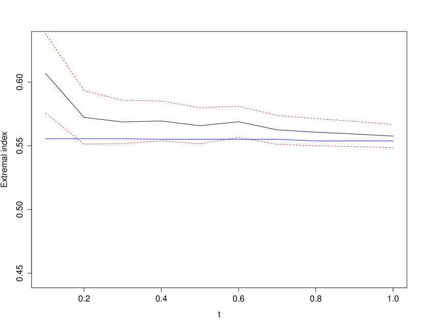
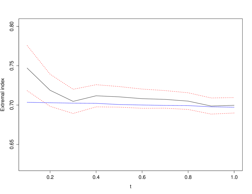
Figure 1: Extremal index for the AR(1)-input

Left: $\theta_{n=10^{4},t}$ is the blue curve, $\widehat{\theta}_{n=10^{4},t}$ is the black curve and the confidence intervals $I_{t}=(CI_{i}(t),CI_{s}(t))$ are the red curves, for the AR(1)-input (2) with $b=2$. Right: the same situation but with $b=3$

t	0.1	0.2	0.3	0.4	0.5	0.6	0.7	0.8	0.9	1.0
$\theta_{n,t}$	0.555	0.555	0.555	0.555	0.555	0.555	0.555	0.553	0.553	0.553
$\widehat{\theta}_{n,t}$	0.606	0.572	0.568	0.569	0.565	0.568	0.562	0.560	0.559	0.557
$CI_{s}$	0.638	0.593	0.585	0.585	0.579	0.581	0.573	0.571	0.569	0.566
$CI_{i}$	0.575	0.551	0.551	0.553	0.551	0.556	0.551	0.549	0.549	0.548

Table 1: Comparison between the blocks estimation and the theoretical approximation (35), for the AR(1)-input with $b=2$ and $n=10^{4}$.

t	0.1	0.2	0.3	0.4	0.5	0.6	0.7	0.8	0.9	1.0
$\theta_{n,t}$	0.703	0.702	0.702	0.702	0.700	0.700	0.699	0.699	0.697	0.697
$\widehat{\theta}_{n,t}$	0.747	0.718	0.704	0.711	0.710	0.708	0.707	0.704	0.698	0.699
$CI_{s}$	0.775	0.739	0.720	0.725	0.723	0.720	0.718	0.715	0.708	0.709
$CI_{i}$	0.718	0.698	0.689	0.697	0.697	0.695	0.696	0.694	0.688	0.689

Table 2: Comparison between the blocks estimation and the theoretical approximation (35), for the AR(1)-input with $b=3$ and $n=10^{4}$

Appendix. $\tau$-weak dependence and proofs

• Brief interlude into $\tau$-weak dependence

Let $(\Omega,\mathcal{A},\mathbb{P})$ be a probability space, and $\mathcal{M}$ a $\sigma$-algebra of $\mathcal{A}$. Let $(E,\delta)$ be a Polish space endowed with its metric. For any $E$-valued random variable $X$, $\mathbb{L}^{p}$-integrable (i.e. $X$ satisfies $\|\delta(X,0)\|_{p}:=\left(\int\delta^{p}(x,0)\mathbb{P}(dx)\right)^{1/p}<\infty$), Dedecker $\&$ Prieur, 2004a defined the coefficient $\tau_{p}$ as:

$$\tau_{p}(\mathcal{M},X):=\|\sup\left\{\mathbb{E}\left[h(X)|\mathcal{M}\right]-\mathbb{E}\left[h(X)\right]:h\in\Lambda(E,\delta)\right\}\|_{p}$$ (36)

where $\Lambda(E,\delta)$ denotes the class of all Lipschitz functions $h:E\longrightarrow\mathbb{R}$ such that

$$\mbox{Lip}(h):=\sup_{x\ y}\frac{|h(x)-h(y)|}{\delta(x,y)}\leq 1.$$

Let $\mathcal{X}=(X_{n,i})_{1\ i\ n,n\in\mathbb{N}}$ be a triangular array of  $\mathbb{L}^{p}$-integrable $E$-valued random variables, and $(\mathcal{M}_{i})_{i\in\mathbb{Z}}$ be a sequence of $\sigma$-algebras of $\mathcal{A}$.
Then, for any $n\in\mathbb{N}$, we define the coefficient:

$$\tau_{p,n}(k):=\sup_{l\ 1}l^{-1}\sup\{\tau_{p}(\mathcal{M}_{i},(X_{n,j_{1}},\ldots,X_{n,j_{l}})):i+k\ j_{1}<\cdots<j_{l}\ n\},$$ (37)

where we consider the distance

$$\delta_{l}(x,y)=\sum_{i=1}^{l}\delta(x_{i},y_{i})$$ (38)

on $E^{l}$. Moreover, we say that $\mathcal{X}$ is $\tau_{p}$-weakly dependent if

$$\lim_{k\longrightarrow\infty}\limsup_{n\longrightarrow\infty}\tau_{p,n}(k)=0.$$ (39)

Remark 3

Recall that $\mathcal{X}=(X_{n,i})_{1\ i\ n,n\in\mathbb{N}}$ is constructed from a random process $\mathbb{X}=(X_{i})_{i\in\mathbb{Z}}$. Therefore the dependence properties of $\mathcal{X}$’s are inherited from those of $\mathbb{X}$. Even more so, if $\mathbb{X}$ is $\tau_{p}$-weakly dependent (in the usual sense defined by Dedecker $\&$ Prieur, 2004a for random processes), then $\mathcal{X}$ is $\tau_{p}$ - weakly dependent with $\tau_{p,n}(\cdot)=L_{n}\cdot\tau_{p}(\cdot)$, for some positive constant $L_{n}$ (which is written in function of $\mathcal{X}$’s normalization constants). For instance, if we consider the normalizations in eqn. (6)-(8) we obtain that $\tau_{p,n}(\cdot)\ a^{-1}_{n}\cdot\tau_{p}(\cdot)$.

In this sense, if we want to study $\mathcal{X}$’s $\tau$-dependence properties, suffice it to take into account $\mathbb{X}$’s $\tau$-dependence properties.

We make use of the previous remark to mention the following examples of $\tau_{p}$-weakly dependent processes without considering the normalizations.

Example 1 (Causal Bernoulli shifts)

Let $(\xi_{i})_{i\in\mathbb{Z}}$ be a sequence of i.i.d.r.v’s. (independent and identically distributed random variables) with values in a measurable space $D$. Assume that there exists a function $H:D^{\mathbb{N}}\longrightarrow\mathbb{R}$, such that $H(\xi_{0},\xi_{-1},\ldots)$ is defined almost surely. Then the stationary sequence $(X_{i})_{i\ 0}$ defined by $X_{i}=H(\xi_{i},\xi_{i-1},\ldots)$ is called a causal Bernoulli shifts.

Let $(\xi^{\prime}_{i})_{i\in\mathbb{Z}}$ be an independent copy of the i.i.d. sequence $(\xi_{i})_{i\in\mathbb{Z}}$. Consider a decreasing sequence $(\Delta_{p}(i))_{i\ 0}$ such that

$$\|X_{i}-X^{\prime}_{i}\|_{p}\ \Delta_{p}(i)$$ (40)

for some $p\in[1,\infty]$, where $X_{i}=H(\xi_{i},\xi_{i-1},\ldots)$ and $X^{\prime}_{i}=H(\xi_{i},\ldots,\xi_{1},\xi^{\prime}_{0},\xi^{\prime}_{-1},\ldots)$. Then, if $\mathcal{M}_{i}=\sigma(X_{j}:j\ i)$, the coefficient $\tau_{p}(k)$ of $(X_{i})_{i\in\mathbb{Z}}$ is bounded above by $\Delta_{p}(k)$, for all $k\in\mathbb{N}$.

Application 1 (Causal linear processes)

Let $D=\mathbb{R}$ and

$$X_{i}=\sum_{j=0}^{\infty}b_{j}\xi_{i-j}.$$ (41)

Here we set $\Delta^{\prime}_{p}(i)=2\|\xi_{0}\|_{p}\sum_{j\ i}|b_{j}|\ \Delta_{p}(i)$ in case $\|\xi_{0}\|_{p}<\infty$.
The model (2) can be write as (41) with $b_{j}=b^{-j-1}$ for some integer $b\ 2$. Since $\xi_{0}$ is uniformly distributed on $U(b)=\{0,\ldots,b-1\}$ in this case, then $X_{0}$ is uniformly distributed over $[0,1]$ and $\Delta_{\infty}(i)\ b^{-i}$.

Example 2 (Markov models)

Let $G:(\mathbb{R}^{l},\mathcal{B}(\mathbb{R}^{l}))\times(D,\mathcal{D})\longrightarrow(\mathbb{R},\mathcal{B}(\mathbb{R}))$ be a measurable function and let $(X_{i})_{i\ 1-l}$ be a sequence of random variables with values in $\mathbb{R}$ such that

$$X_{i}=G(X_{i-1},X_{i-2},\ldots,X_{i-l};\xi_{i}),\qquad\forall i\ 1,$$ (42)

for some sequence $(\xi_{i})_{i\in\mathbb{N}}$ of i.i.d.r.v’s. with values in a measurable space $D$ and independent of $(X_{0},\ldots,X_{1-l})$. Then the random variables $Y_{i}=(X_{i},X_{i-1},\ldots,X_{i-l+1})$ defines a Markov chain such that $Y_{i}=F(Y_{i-1};\xi_{i})$ with

$$F(x_{l},\ldots,x_{1};\xi):=(G(x_{l},\ldots,x_{1};\xi),x_{l},x_{l-1},\ldots,x_{2}).$$ (43)

Assume that $Y_{0}=(X_{0},\ldots,X_{1-l})$ is a stationary solution of (42). Let $Y^{\prime}_{0}=(X^{\prime}_{0},\ldots,X^{\prime}_{1-l})$ be independent of $(Y_{0},(\xi_{i})_{i\in\mathbb{N}})$ and distributed as $Y_{0}$. Then setting

$$X^{\prime}_{i}=G(X^{\prime}_{i-1},\ldots,X^{\prime}_{i-l};\xi_{i}),$$ (44)

$X^{\prime}_{i}$ is distributed as $X_{i}$ and it is independent of $\mathcal{M}_{0}=\sigma(X_{0},\ldots,X_{1-l})$, for all $i\in\mathbb{N}$. As in the previous example, let $(\Delta_{p}(i))_{i\ 0}$ be a non increasing sequence such that (40) holds, with $X_{i}$ and $X^{\prime}_{i}$ defined in (42) and (44), respectively. Hence one can apply the result of Lemma 3 in [Dedecker $\&$ Prieur, 2004a, ], and we obtain that $\tau_{p}(k)\ \Delta_{p}(k)$.

In particular if $G$ is such that

$$\|G(x;\xi_{1})-G(y;\xi_{1})\|_{p}\ \sum_{i=1}^{l}a_{i}|x_{i}-y_{i}|\text{, \quad with }\sum_{i=1}^{l}a_{i}<1,$$ (45)

then $\Delta_{p}(k)\ Ca^{k}$ for some $a\in[0,1)$ and some $C>0$. (see [Dedecker et al.,, 2007], page 34).

Application 2 (Contracting Markov chain)

Let $X_{i}=G(X_{i-1},\xi_{i})$ be a Markov chain such that $G:(\mathbb{R},\mathcal{B}(\mathbb{R}))\times(D,\mathcal{D})\longrightarrow(\mathbb{R},\mathcal{B}(\mathbb{R}))$ is a measurable function and

$$A=\|G(0;\xi_{1})\|_{p}<\infty\text{ and }\|G(x;\xi_{1})-G(y;\xi_{1})\|_{p}\ a|x-y|,$$ (46)

for some $a\in(0,1)$ and some $p\in[1,\infty]$. Then, $(X_{i})_{i\in\mathbb{N}}$ has a stationary solution with $p$-th order finite moment as this is proved on page 35 of Dedecker et al., [2007]. Moreover under this condition: $\Delta_{p}(k)=\|X^{\prime}_{0}-X_{0}\|_{p}\cdot a^{k}$.

Remark 4

In particular if $G(u;\xi)=A(u)+B(u)\xi$ for suitable Lipschitz functions $A(u)$ and $B(u)$ with $u\in\mathbb{R}$, then the corresponding iterative model (ARCH-type process) $X_{i}=G(X_{i-1};\xi_{i})$ satisfies (46) with $a=\mbox{Lip}(A)+\|\xi_{1}\|_{p}\mbox{Lip}(B)<1$.

Remark 5

The stationary iterative models $X_{i}=G(X_{i-1},\xi_{i})$ are causal Bernoulli shifts if the condition (46) holds; this is proved in Proposition 3.2 in [Dedecker et al.,, 2007].

Application 3 (Nonlinear AR($l$)-models)

Let $l\geq 1$ and $(X_{i})_{i}$ be the stationary solution of some equation

$$X_{i}=R(X_{i-1},\ldots,X_{i-l})+\xi_{i}$$

for some measurable function $R:\mathbb{R}^{l}\to\mathbb{R}$. The process $(X_{i})_{i}$ is then called a stationary real nonlinear autoregressive model of order $l$. If $\|\xi_{1}\|_{p}<\infty$ and

$$|R(u_{1},\ldots,u_{l})-R(v_{1},\ldots,v_{l})|\ \sum_{i=1}^{l}a_{i}|u_{i}-v_{i}|,\mbox{ for }a_{1},\ldots,a_{l}\ 0\mbox{ with }\sum_{i=1}^{l}a_{i}<1,$$

and for all $(u_{1},\ldots,u_{l}),(v_{1},\ldots,v_{l})\in\mathbb{R}^{l}$, then the function $G:\mathbb{R}^{l+1}\to\mathbb{R}$ defined by $G(u;\xi)=R(u)+\xi$ satisfies Condition (45) and therefore the sequence $(\Delta_{p}(k))_{k}$ admits an exponential decay rate.

• Coupling

Let $d_{\cup}:E_{\cup}\times E_{\cup}\longrightarrow[0,\infty)$ be a pseudometric defined as follows: let $x_{k}=(x_{k}^{(1)},x_{k}^{(2)},\ldots,x_{k}^{(r_{k})})\in E_{\cup}$ for $k=1,2$ and we denote

$$x_{{}_{1,2}}=\left\{\begin{array}[]{ll}x_{1},&\mbox{if $r_{1}\ r_{2}$},\\ (x_{1}^{(1)},\ldots,x_{1}^{(r_{1})},x_{2}^{(r_{1}+1)},\ldots,x_{2}^{(r_{2})}),&\mbox{if $r_{1}<r_{2}$}.\end{array}\right.$$

Similarly is denoted $x_{{}_{2,1}}$. Then,

$$d_{\cup}(x_{1},x_{2}):=d_{r_{1}\vee r_{2}}(x_{{}_{1,2}},x_{{}_{2,1}}),$$ (47)

where $d_{r}(\cdot,\cdot)$ is defined in (38).

Lemma 2 (Coupling: the even and odd blocks)

Suppose that the random variables $(X_{n,i})_{1\ i\ n}$ are such that (B.2) holds. We consider together even and odd block sizes, by using $k=0$ or $1$ according to the parity. Assume that for each $j\in\{2,\ldots,[m_{n}/2]\}$ there is a random variable $U_{k,j}$ uniformly distributed on $[0,1]$ and independent of $\mathcal{M}_{n,j-1}^{k}=\sigma(Y_{n,2-k},\ldots,Y_{n,2(j-1)-k)})$ and $\sigma(Y_{n,2j-k})$. Then there exists a random block $\dot{Y}_{n,2j-k}$ measurable with respect to $\mathcal{M}_{n,j-1}^{k}\vee\sigma(Y_{n,2j-k})\vee\sigma(U_{k,j})$, independent of $\mathcal{M}_{n,j-1}^{k}$ and distributed as $Y_{n,2j-k}$ such that

$$\left\|\left.\mathbb{E}\left(d_{\cup}(Y_{n,2j-k},\dot{Y}_{n,2j-k})\right)\right|\mathcal{M}_{n,j-1}^{k}\right\|_{1}\ r_{n}\tau_{1,n}(r_{n}).$$ (48)

In particular, if we set $\mathcal{M}_{n,j-1}^{k}=\sigma(\dot{Y}_{n,2-k},\ldots,\dot{Y}_{n,2(j-1)-k})$, then the blocks $(\dot{Y}_{n,2j-k})_{1\ j\ [m_{n}/2]}$ are independent.

Proof: We set here $k=0$ (for even block sizes) since the steps are similar if $k=1$.
Let $Y_{n,2j}=(X_{n,i})_{i\in A_{j}}$ be a random block, where$A_{j}=\{(2j-1)r_{n}+1,\ldots,2jr_{n}\}$. Then, from Dedecker et al., [2007]’s Lemma 5.3, there exists a random random block $\dot{Y}_{n,2j}\in E^{r_{n}}$ measurable with respect to $\mathcal{M}_{n,j-1}^{0}\vee\sigma(Y_{n,2j})\vee\sigma(U_{0,j})$ independent of $\mathcal{M}_{n,j-1}^{0}$ and distributed as $Y_{n,2j}$ such that

$$\tau_{p}(\mathcal{M}^{0}_{n,j-1},Y_{n,2j})=\left\|\mathbb{E}(d_{r_{n}}(Y_{n,2j},\dot{Y}_{n,2j})\left|\mathcal{M}^{0}_{n,j-1})\right.\right\|_{p}.$$ (49)

Therefore,

$$\left\|\mathbb{E}(d_{\cup}\left(Y_{n,2j},\dot{Y}_{n,2j}\right)\left|\mathcal{M}^{0}_{n,j-1})\right.\right\|_{1}=\left\|\mathbb{E}(d_{r_{n}}\left(Y_{n,2j},\dot{Y}_{n,2j}\right)\left|\mathcal{M}^{0}_{n,j-1})\right.\right\|_{1}\\ =\tau_{1}(\mathcal{M}^{0}_{n,j-1},Y_{n,2j})\leq r_{n}\tau_{1,n}(r_{n}).\ \ \square$$ (50)

Lemma 3 (Coupling: the sub-blocks)

Suppose that the random variables $(X_{n,i})_{1\ i\ n}$ are such (B.2) holds. Moreover, if that for each $j\in\{2,\ldots,[m_{n}/2]\}$ there is a random variable $U_{k,j}$ uniformly distributed on $[0,1]$ and independent of the $\sigma-$algebras $\mathcal{M}_{n,j-1}=\sigma(Y_{n,1}^{[r_{n}-l_{n}]},\ldots,Y_{n,j-1}^{[r_{n}-l_{n}]})$ and $\sigma(Y_{n,j}^{[r_{n}-l_{n}]})$. Then there exists a random block $\dot{Y}_{n,j}^{[r_{n}-l_{n}]}$, measurable with respect to $\mathcal{M}_{n,j-1}\vee\sigma(Y_{n,j}^{[r_{n}-l_{n}]})\vee\sigma(U_{j})$, independent of $\mathcal{M}_{n,j-1}$ and distributed as $Y_{n,j}^{[r_{n}-l_{n}]}$ such that

$$\left\|\left.\mathbb{E}\left(d_{\cup}(Y_{n,j}^{[r_{n}-l_{n}]},\dot{Y}_{n,j}^{[r_{n}-l_{n}]})\right)\right|\mathcal{M}_{n,j-1}\right\|_{1}\ r_{n}\tau_{1,n}(l_{n}).$$ (51)

Moreover, if we set $\mathcal{M}_{n,j-1}=\sigma(\dot{Y}_{n,1}^{[r_{n}-l_{n}]},\ldots,\dot{Y}_{n,j-1}^{[r_{n}-l_{n}]})$ then the blocks $(\dot{Y}_{n,j}^{[r_{n}-l_{n}]})_{1\ j\ m_{n}}$ are independent.

Proof. The same argument previous proof. However note that the sub-blocks $(Y_{n,j}^{[r_{n}-l_{n}]})_{1\ j\ m_{n}}$ are separated by $l_{n}$ variables. $\square$

• Proof of Theorem 1

Let $(Y_{n,j})_{1\ j\ m_{n}}$ be the blocks built from $(X_{n,i})_{1\ i\ n}$. For $k\in\{0,1\}$, we consider the independent blocks $(\dot{Y}_{n,2j-k})_{1\ j\ [m_{n}/2]}$ coupled to the original blocks $(Y_{n,2j-k})_{1\ j\ [m_{n}/2]}$, from Lemma 2. Therefore, if we define $\Delta_{n,j}^{*}:=f(\dot{Y}_{n,j})-f(\dot{Y}_{n,j}^{(r_{n}-l_{n})})$, for $j=1,\ldots,m_{n}$, we have that $\Delta_{n,j}^{*}(f)\overset{\mathcal{D}}{=}\Delta_{n,j}(f)\overset{\mathcal{D}}{=}\Delta_{n}(f)$, for each $j$, where $\Delta_{n,j}(f):=f(Y_{n,j})-f(Y_{n,j}^{(r_{n}-l_{n})})$ and $\Delta_{n}(f)$ is defined in (11). Now, if we consider the assumption (C.1), we can apply Petrov, [1975]’s Theorem 1 (Section IX.1) to the i.i.d.r.v’s $X_{n,j}:=(nv_{n})^{-1/2}\Delta_{n,j}^{*}(f)$, so

$$D\dot{Z}_{n}^{(k)}(f):=\dfrac{1}{\sqrt{nv_{n}}}\sum_{j=1}^{[m_{n}/2]}\left(\Delta^{*}_{n,2j-k}(f)-\mathbb{E}\Delta^{*}_{n,2j-k}(f)\right)=o_{P}(1)$$ (52)

for $k=0,1$. In consequence,

$$DZ_{n}(f):=\dfrac{1}{\sqrt{nv_{n}}}\sum_{j=1}^{m_{n}}\left(\Delta_{n,j}(f)-\mathbb{E}\Delta_{n,j}(f)\right)=o_{P}(1)$$ (53)

On the other hand, by Lemma 3, we have that

$$BZ_{n}(f):=\dfrac{1}{\sqrt{nv_{n}}}\sum_{j=1}^{m_{n}}\left(f(Y_{n,j}^{(r_{n}-l_{n})})-\mathbb{E}f(Y_{n,j}^{(r_{n}-l_{n})})\right)$$ (54)

converge weakly in fidis if, and only if

$$B\dot{Z}_{n}(f):=\dfrac{1}{\sqrt{nv_{n}}}\sum_{j=1}^{m_{n}}\left(f(\dot{Y}_{n,j}^{(r_{n}-l_{n})})-\mathbb{E}f(\dot{Y}_{n,j}^{(r_{n}-l_{n})})\right)$$ (55)

converge weakly in fidis (and in this case the limit distributions are the same). The latter holds because $B\dot{Z}_{n}(f)=\dot{Z}_{n}(f)-D\dot{Z}_{n}(f)$ and from the assumptions (C.2) and (C.3), where

$$\dot{Z}_{n}(f):=\dfrac{1}{\sqrt{nv_{n}}}\sum_{j=1}^{m_{n}}\left(f(\dot{Y}_{n,j})-\mathbb{E}f(\dot{Y}_{n,j})\right).$$

Finally, as $Z_{n}(f)=BZ_{n}(f)+DZ_{n}(f)$ $\forall f\in\mathcal{F}$, we get the result. $\square$

• Proof of Proposition 1

Suffices to prove the following multidimensional version of Segers, [2003]’s condition (6):

$$\lim_{l\to\infty}\limsup_{n\to\infty}\mathbb{P}\left\{Y_{n}^{[l+1:r_{n}]}\ 0|X_{n,1}\ 0\right\}=0,$$ (56)

since the rest of the proof follows the same steps of the proof of Drees $\&$ Rootzén, [2010]’s Lemma 5.2.

Indeed, let $h(\cdot)=\mathbb{1}\{\cdot\ 0\}$ be a function defined on $E^{r_{n}-l}$. Consider a increasing sequence of functions $h_{k}(\cdot):E^{r_{n}-l}\longrightarrow[0,1]$ which approximate to $h$, and such that $\mbox{Lip}(h_{k})=v_{k}^{-\alpha}$ for some $\alpha>0$. Of course, we set $k=k(n)\ll n$. Then,

$$\limsup_{n\to\infty}\mathbb{P}\{Y_{n}^{(l+1:r_{n})}\ 0|X_{n,1}\ 0\}=\limsup_{n\to\infty}v_{n}^{-1}\mathbb{P}\{Y_{n}^{(l+1:r_{n})}\ 0,X_{n,1}\ 0\}\\ =\limsup_{n\to\infty}v_{n}^{-1}\int_{\{X_{n,1}\ 0\}}\mathbb{P}\{Y_{n}^{(l+1:r_{n})}\ 0|\sigma(X_{n,1})\}d\mathbb{P}\\ =\limsup_{n\to\infty}v_{n}^{-1}\int_{\{X_{n,1}\ 0\}}\mathbb{E}[\mathbb{1}\{Y_{n}^{(l+1:r_{n})}\ 0\}|\sigma(X_{n,1})]d\mathbb{P}\\ =\limsup_{k\to\infty}\dfrac{v_{n}^{-1}}{v_{k}^{\alpha}}\int_{\{X_{n,1}\ 0\}}\mathbb{E}\left[\dfrac{h_{k}(Y_{n}^{[l+1:r_{n}]})}{v_{k}^{-\alpha}}|\sigma(X_{n,1})\right]d\mathbb{P}\\ \ \limsup_{k\to\infty}\dfrac{1}{v_{k}^{\alpha+1/p}}\left\|\mathbb{E}\left[\dfrac{h_{k}(Y_{n}^{[l+1:r_{n}]})}{v_{k}^{-\alpha}}|\sigma(X_{n,1})\right]\right\|_{p}\\ \ \limsup_{k\to\infty}\left[\dfrac{(r_{n}-l)}{v_{k}^{\alpha+1/p}}\tau_{n,p}(l)+(r_{n}-l)v_{n}^{1/q}\right]\ \limsup_{k\to\infty}\dfrac{r_{n}\tau_{n,p}(l)}{v_{k}^{\alpha+1/p}}.$$

Finally, taking $l\to\infty$ we have the limit (56) proven. $\square$

• Proof of Theorem 2

Note that $Z_{n}$ is asymptotically tight iff $\dot{Z}_{n}^{(k)}$ defined by:

$$Z_{n}^{(k)}(f):=\dfrac{1}{\sqrt{nv_{n}}}\sum_{j=1}^{[m_{n}/2]}\left(f(Y_{n,2j-k})-\mathbb{E}f(Y_{n,2j-k})\right)$$ (57)

is asymptotically tight for each $k\in\{0,1\}$. On the other hand, for each $k\in\{0,1\}$ we use Lemma 2 together with (B.2) and (D.1) conditions to build independent blocks $(\dot{Y}_{n,2j-k})_{1\ j\ [m_{n}/2]}$ coupled to the original blocks $(Y_{n,2j-k})_{1\ j\ [m_{n}/2]}$. In this manner we have that $Z_{n}^{(k)}$ is asymptotically tight iff

$$\dot{Z}_{n}^{(k)}(f):=\dfrac{1}{\sqrt{nv_{n}}}\sum_{j=1}^{[m_{n}/2]}\left(f(\dot{Y}_{n,2j-k})-\mathbb{E}f(\dot{Y}_{n,2j-k})\right)$$ (58)

is asymptotically tight, for each $k\in\{0,1\}$. The latter is true due to Theorem 2.11.9 in [Van Der Vaart $\&$ Wellner,, 1996] by setting $Z_{nj}(f)=f(Y_{n,j})$ and $[m_{n}/2]$ instead of $m_{n}$.

For the remaining assertion we use Theorem 1. $\square$

• Proof of Theorem 3

Consider (T.5). Note that from the triangle inequality $Z_{n}$ is asymptotically equicontinuous if $\dot{Z}^{(k)}_{n}$ from eqn. (57) is asymptotically equicontinuous for each $k\in\{0,1\}$. Now, again we use Lemma 2 together with (B.2) and (D.1) conditions as in the previous proof to prove that $Z_{n}^{(k)}$ is asymptotically equicontinuous iff $\dot{Z}_{n}^{(k)}$ is asymptotically equicontinuous for each $k\in\{0,1\}$. However, in this case $\dot{Z}_{n}^{(k)}$ is asymptotically equicontinuous from Theorem 2.11.1 in [Van Der Vaart $\&$ Wellner,, 1996].
The remaining steps are the same of Theorem 2.10’s proof in [Drees $\&$ Rootzén,, 2010]. $\square$

• Proof of Proposition 2

The steps are the same that in the proof of Theorem 2.1 in [Drees,, 2011], but replacing the assumptions (C1) and (C2) of his paper by our assumptions (B.2) and (B.1), respectively.

$\square$

• Proof of Corollary 3

Suffices to replace the assumptions (C1) and (C2) in the proof of Drees, [2011]’s Corollary 2.3 by our assumptions (B.2) and (B.1) respectively. $\square$

• Proof of the expression (4.1)

If $(X_{i})_{i\ 0}$ is the AR(1)-process (2), note that for each $i\in\mathbb{N}$

$$X_{i}=\dfrac{X_{0}}{b^{i}}+\sum_{s=1}^{i}\dfrac{\xi_{s}}{b^{i-s+1}}.$$ (59)

Therefore, if $n$ is sufficiently large such that $b^{d}v_{n}<1$, then for $x\in[0,1]^{d}$:

$$\mathbb{P}\{X_{n,1}>x,X_{n,1}\ 0\}=\mathbb{P}\{X_{i}>a_{n}x_{i}+u_{n},\text{ for some }i=1,\ldots,d\}\\ =\mathbb{P}\left\{X_{0}>b^{i}(a_{n}x_{i}+u_{n})-\sum_{s=1}^{i}b^{s-1}\xi_{s},\text{ for some }i=1,\ldots,d\right\}$$

$$=\mathbb{P}\left\{X_{0}>\min_{i=1,\ldots,d}\left\{b^{i}(a_{n}x_{i}+u_{n})-\sum_{s=1}^{i}b^{s-1}\xi_{s}\right\}\right\}\\ =\sum_{j_{1},\ldots,j_{d}\in U(b)}\mathbb{P}\left\{X_{0}>\min_{i=1,\ldots,d}\left\{b^{i}(a_{n}x_{i}+u_{n})-\sum_{s=1}^{i}b^{s-1}j_{s}\right\},(\xi_{1},\ldots,\xi_{d})=(j_{1},\ldots,j_{d})\right\}\\ =\dfrac{1}{b^{d}}\sum_{j_{1},\ldots,j_{d}\in U(b)}\mathbb{P}\left\{X_{0}>\min_{i=1,\ldots,d}\left\{b^{i}(a_{n}x_{i}+u_{n})-\sum_{s=1}^{i}b^{s-1}j_{s}\right\}\right\}\\ =\dfrac{1}{b^{d}}\sum_{j_{1},\ldots,j_{d}\in U(b)}\left(\max_{i=1,\ldots,d}\left\{1-b^{i}+\sum_{s=1}^{i}b^{s-1}j_{s}+b^{i}v_{n}(1-x_{i})\right\}_{+}\land 1\right)\\ =\dfrac{1}{b^{d}}\max_{i=1,\ldots,d}\left\{b^{i}v_{n}(1-x_{i})\right\},$$

since $\mu_{b}(j_{1},\ldots,j_{d};i):=1-b^{i}+\sum_{s=1}^{i}b^{s-1}j_{s}\ -1$ for all $(j_{1},\ldots,j_{d})\in U^{d}(b)\setminus\{(b-1,\ldots,b-1)\}$ and $\mu_{b}(b-1,b-1,\ldots,b-1)=0$. Thus,

$$\mathbb{P}\{X_{n,1}>x|X_{n,1}\ 0\}\underset{{}_{n\to\infty}}{\longrightarrow}\max_{i=1,\ldots,d}\{b^{i-d}(1-x_{i})\}.$$ (60)

$\square$

• Proof of the expression (4.1)

Let $x,y\in[0,1]^{d}$. Then as before for $i\ 1$, if $n$ is sufficiently large such that $b^{i+d}v_{n}<1$, then we have:

$$\mathbb{P}\{X_{n,1}>x,X_{n,i+1}>y\}\\ =\mathbb{P}\left\{X_{k}>a_{n}x_{k}+u_{n},X_{i+l}>a_{n}y_{l}+u_{n},\text{ for some }(k,j)\in\{1,\ldots,d\}^{2}\right\}\\ =\mathbb{P}\left\{X_{0}>\min_{k=1,\ldots,d}\left\{b^{k}(a_{n}x_{k}+u_{n})-\sum_{s=1}^{k}b^{s-1}\xi_{s}\right\},\right.\\ \left.X_{i}>\min_{l=1,\ldots,d}\left\{b^{l}(a_{n}y_{l}+u_{n})-\sum_{s=1}^{l}b^{s-1}\xi_{s+i}\right\}\right\}\\ =\sum_{\overset{j_{1},\ldots,j_{d}\in U(b)}{j_{i+1},\ldots,j_{i+d}\in U(b)}}\mathbb{P}\left\{X_{0}>\min_{k=1,\ldots,d}\left\{b^{k}(a_{n}x_{k}+u_{n})-\sum_{s=1}^{k}b^{s-1}j_{s}\right\},\right.\\ X_{i}>\min_{l=1,\ldots,d}\left\{b^{l}(a_{n}y_{l}+u_{n})-\sum_{s=1}^{l}b^{s-1}j_{s+i}\right\},\\ \left.(\xi_{1},\ldots,\xi_{d},\xi_{i+1},\ldots,\xi_{i+d})=(j_{1},\ldots,j_{d},j_{i+1},\ldots,j_{i+d})\right\}$$

$$=\dfrac{1}{b^{d}}\sum_{\overset{j_{1},\ldots,j_{d}\in U(b)}{j_{i+1},\ldots,j_{i+d}\in U(b)}}\mathbb{P}\left\{X_{0}>\min_{k=1,\ldots,d}\left\{b^{k}(a_{n}x_{k}+u_{n})-\sum_{s=1}^{k}b^{s-1}j_{s}\right\},\right.\\ \left.X_{i}>\min_{l=1,\ldots,d}\left\{b^{l}(a_{n}y_{l}+u_{n})-\sum_{s=1}^{l}b^{s-1}j_{s+i}\right\},(\xi_{1},\ldots,\xi_{d})=(j_{1},\ldots,j_{d})\right\}\\ =\dfrac{1}{b^{d}}\sum_{\overset{j_{1},\ldots,j_{d}\in U(b)}{j_{i+1},\ldots,j_{i+d}\in U(b)}}\mathbb{P}\left\{X_{0}>1-\max_{k=1,\ldots,d}\left\{\mu_{b}(j_{1},\ldots,j_{d};k)+b^{k}v_{n}(1-x_{k})\right\}_{+}\land 1,\right.\\ \left.X_{i}>1-\max_{l=1,\ldots,d}\left\{\mu_{b}(j_{i+1,\ldots,j_{i+d}})+b^{l}v_{n}(1-y_{l})\right\}_{+}\land 1,(\xi_{1},\ldots,\xi_{d})=(j_{1},\ldots,j_{d})\right\}\\ =\dfrac{1}{b^{d}}\mathbb{P}\left\{X_{0}>1-\max_{k=1,\ldots,d}\left\{b^{k}v_{n}(1-x_{k})\right\},\right.\\ \left.X_{i}>1-\max_{l=1,\ldots,d}\left\{b^{l}v_{n}(1-y_{l})\right\},\xi_{1}=\ldots=\xi_{d}=b-1\right\}$$

since $\mu_{b}(j_{1},\ldots,j_{d};i):=1-b^{i}+\sum_{s=1}^{i}b^{s-1}j_{s}\ -1$ for all $(j_{1},\ldots,j_{d})\in U^{d}(b)\setminus\{(b-1,\ldots,b-1)\}$ and $\mu_{b}(b-1,b-1,\ldots,b-1)=0$.

Moreover, note that if $i>d$

$$\mathbb{P}\{X_{n,1}>x,X_{n,i+1}>y\}=\dfrac{1}{b^{d}}\mathbb{P}\left\{X_{0}>1-\max_{k=1,\ldots,d}\left\{b^{k}v_{n}(1-x_{k})\right\},\right.\\ \left.X_{i}>1-\max_{l=1,\ldots,d}\left\{b^{l}v_{n}(1-y_{l})\right\},\xi_{1}=\ldots=\xi_{d}=b-1\right\}\\ =\dfrac{1}{b^{d}}\mathbb{P}\left\{X_{0}>1-\max_{k=1,\ldots,d}\left\{b^{k}v_{n}(1-x_{k})\right\},\right.\\ \left.X_{0}>b^{i}-b^{i}\max_{l=1,\ldots,d}\left\{b^{l}v_{n}(1-y_{l})\right\}+1-b^{d}-\sum_{s=d+1}^{i}b^{s-1}\xi_{s}\right\}\\ =\dfrac{1}{b^{d}}\sum_{j_{d+1,\ldots,j_{i}}\in U(b)}\mathbb{P}\left\{X_{0}>1-\max_{k=1,\ldots,d}\left\{b^{k}v_{n}(1-x_{k})\right\},\right.\\ \left.X_{0}>b^{i}-b^{i}\max_{l=1,\ldots,d}\left\{b^{l}v_{n}(1-y_{l})\right\}+1-b^{d}-\sum_{s=d+1}^{i}b^{s-1}j_{s},(\xi_{d+1},\ldots,\xi_{i})=(j_{d+1},\ldots,j_{i})\right\}\\ =\dfrac{1}{b^{i}}\sum_{j_{d+1,\ldots,j_{i}}\in U(b)}\mathbb{P}\left\{X_{0}>1-\max_{k=1,\ldots,d}\left\{b^{k}v_{n}(1-x_{k})\right\},\right.\\ \left.X_{0}>b^{i}-b^{i}\max_{l=1,\ldots,d}\left\{b^{l}v_{n}(1-y_{l})\right\}+1-b^{d}-\sum_{s=d+1}^{i}b^{s-1}j_{s}\right\}$$

$$=\dfrac{1}{b^{i}}\sum_{j_{d+1,\ldots,j_{i}}\in U(b)}\min\left(\max_{k=1,\ldots,d}\left\{b^{k}v_{n}(1-x_{k})\right\},\right.\\ \left.\max_{l=1,\ldots,d}\left\{b^{d}+\sum_{s=d+1}^{i}b^{s-1}j_{s}+b^{l+i}v_{n}(1-y_{l})-b^{i}\right\}_{+},1\right)\\ \\ =\dfrac{v_{n}}{b^{i}}\min\left(\max_{k=1,\ldots,d}\left\{b^{k}(1-x_{k})\right\},\max_{l=1,\ldots,d}\left\{b^{l+i}(1-y_{l})\right\}\right)=v_{n}H_{b,i}(x,y)$$

Similarly for $1\ i<d$, we obtain that

$$\mathbb{P}\{X_{n,1}>x,X_{n,i+1}>y\}\\ =\dfrac{v_{n}}{b^{i}}\min\left(\max_{k=1\ldots,i}\{b^{k}(1-x_{k})\},\max_{k=i+1,\ldots,d}\{b^{k}\min(1-x_{k},1-y_{k})\},\max_{k=d-i,\ldots,d}\{b^{k+i}(1-y_{k})\}\right)\\ =v_{n}H_{b,i}(x,y)$$

From Lemma 5.2 - (iii) in [Drees $\&$ Rootzén,, 2010], $\mathbb{E}|f(Y_{n})|=o(\sqrt{nv_{n}})$. Thus, for $n$ sufficiently large:

$$\dfrac{\mbox{Cov}\left(f_{x}(Y_{n}),f_{y}(Y_{n})\right)}{r_{n}v_{n}}\sim\mathbb{P}\{X_{n,1}>x,X_{n,1}>y\}\\ +\sum_{i=1}^{r_{n}-1}\left(1-\frac{i}{r_{n}}\right)\left(\mathbb{P}\{X_{n,1}>x,X_{n,i+1}>y\}+\mathbb{P}\{X_{n,1}>y,X_{n,i+1}>x\}\right)\\ \underset{{}_{n\to\infty}}{\longrightarrow}\min\left(\max_{k=1,\ldots,d}\{b^{k}(1-x_{k})\},\max_{k=1,\ldots,d}\{b^{k}(1-y_{k})\}\right)+\sum_{i=1}^{\infty}\left(H_{b,i}(x,y)+H_{b,i}(y,x)\right).$$

$\square$

• Proof of the expression (35)

The proof is similar to the proof of the expression (4.1). Indeed,

$$\mathbb{P}\left\{\max_{1\ i\ r_{n}}X_{i}>1-v_{n}t\right\}=\mathbb{P}\left\{X_{i}>1-v_{n}t,\text{ for some }i=1,\ldots,r_{n}\right\}\\ =\mathbb{P}\left\{X_{0}>b^{i}(1-v_{n}t)-\sum_{s=1}^{i}b^{s-1}\xi_{s},\text{ for some }i=1,\ldots,r_{n}\right\}\\ =\mathbb{P}\left\{X_{0}>\min_{1\ i\ r_{n}}\left\{b^{i}(1-v_{n}t)-\sum_{s=1}^{i}b^{s-1}\xi_{s}\right\}\right\}$$

$$=\sum_{j_{1},\ldots,j_{r_{n}}\in U(b)}\mathbb{P}\left\{X_{0}>\min_{1\ i\ r_{n}}\left\{b^{i}(1-v_{n}t)-\sum_{s=1}^{i}b^{s-1}\xi_{s}\right\},(\xi_{1},\ldots,\xi_{r_{n}})=(j_{1},\ldots,j_{r_{n}})\right\}\\ =\dfrac{1}{b^{r_{n}}}\sum_{j_{1},\ldots,j_{r_{n}}\in U(b)}\mathbb{P}\left\{X_{0}>\min_{1\ i\ r_{n}}\left\{b^{i}(1-v_{n}t)-\sum_{s=1}^{i}b^{s-1}j_{s}\right\}\right\}\\ =\dfrac{1}{b^{r_{n}}}\sum_{j_{1},\ldots,j_{r_{n}}\in U(b)}\min\left(\max_{1\ i\ r_{n}}\left\{1+\sum_{s=1}^{i}b^{s-1}j_{s}-b^{i}(1-v_{n}t)\right\}_{+},1\right).$$

$\square$

Aknowledgements.

Warm thanks are due to the very constructive and friendly help of Olivier Wintenberger in the redaction and the finalization of this paper.
Very specials thanks are also due to an anonymous referee who pointed clearly the weaknesses of a previous version of this work and helped us to make it more adequate for publication.

References

- Andrews, [1984] Andrews, D. Non strong mixing autoregressive processes. J. Appl. Probab. 21, 930-934; (1984).
- Ango Nze Doukhan, [2004] Ango Nze P. Doukhan P. Weak dependence and applications to econometrics. Econom Theory 20: 995 - 1045; (2004).
- Basrak Segers, [2009] Basrak, B. Segers, J. Regularly varying multivariate time series. Stoch. Proc. Appl. 119, 1055 - 1080; (2009).
- [4] Dedecker, J. Prieur, C. Coupling for dependent sequences and applications. Journal of Theor. Probab. 17-4, 861-885; (2004a).
- [5] Dedecker, J., Prieur, C. Couplage pour la distance minimale. C. R. Acad. Sci. Paris Serie 1 338-10, 805-808; (2004)
- Dedecker Prieur, [2005] Dedecker, J., Prieur, C. New dependence coefficients. Examples and applications to statistics. Prob. Theor. and Rel. Fields 132, 203-236; (2005).
- Dedecker et al., [2007] Dedecker, J., Doukhan, P., Lang, G., León, J.R., Louhichi,S. Prieur, C. Weak dependence: With Examples and Applications Lecture Notes in Statistics 190, Springer-Verlag; (2007).
- Doukhan, [1994] Doukhan, P. Mixing: Properties and Examples.. Lect. Notes Statis. 85; (1994).
- Doukhan Louhichi, [1999] Doukhan, P. Louhichi, S. A new weak dependence condition and applications to moment inequalities.Stoch. Proc. Appl. 84. 313-342; (1999).
- Doukhan et al., [2006] Doukhan, P., Teyssiere, G. and Winant, P. Vector valued ARCH() - processes, in Dependence in Probability and Statistics, P. Bertail, P. Doukhan and P. Soulier Eds. Lecture Notes in Statistics, Springer, New York (2006).
- Doukhan, [2015] Doukhan, P. Stochastic Models for Time Series. Springer-Verlag; (2015).
- Drees, [2000] Drees, H. Weighted Approximations of Tail Processes for -Mixing Random Variables. Ann. Appl. Probab. 10, 1274-1301; (2000).
- Drees, [2002] Drees, H. Tail empirical processes under mixing conditions. In: H.G. Dehling, T. Mikosch and M. Sorensen (eds.), Empirical Process Techniques for Dependent Data, 325-342. Birkhuser, Boston; (2002).
- Drees, [2003] Drees, H. Extreme Quantile Estimation for Dependent Data with Applications to Finance. Bernoulli 9, 617-657; (2003).
- Drees Rootzén, [2010] Drees, H Rootzén, H. Limit Theorems for Empirical Processes of Cluster Functionals. Ann. Stat. 4, 2145 - 2186; (2010).
- Drees, [2011] Drees, H. Bias correction for blocks estimators of the extremal index. Univ. Hamburg; (2011).
- Eberlein, [1984] Eberlein, E. Weak convergence of partial sums of absolutely regular sequences. Statist. Probab. Letters 2, 291 - 293; (1984).
- Gómez, [2015] Gómez, J.G. Dependent Lindeberg CLT - Finite Dimensional for Empirical Processes of Cluster Functionals. Preprint in arXiv:1404.4989; (2015).
- Perfekt, [1994] Perfekt, R. Extremal behaviour of stationary Markov chains with applications. Ann. Appl. Prob. 4, 529 - 548; (1994).
- Petrov, [1975] Petrov, V.V. Sums of Independent Random Variables. Springer, Berlin; (1975).
- Pickands, [1975] Pickands, J. Statistical inference using extreme order statistics. Ann. Statist. 3, 119-131; (1975).
- Rootzén, [1995] The tail empirical process for stationary sequences. Technical report, Department of Mathematics, Chalmers University, Sweden; (1995).
- Rootzén, [2009] Rootzén, H. Weak convergence of the tail empirical function for dependent sequences. Stoch. Proc. Appl. 119, 468 - 490; (2009).
- Segers, [2003] Segers, J. Functionals of clusters of extremes. Adv. Appl. Probab. 35, 1028 - 1045; (2003).
- Yun, [1998] Yun, S. The extremal index of a higher-order stationary Markov chain. Ann. Appl. Prob. 8. 408 - 437; (1998).
- Yun, [2000] Yun, S. The distribution of cluster functionals of extreme events in a dth-order Markov chain. J. Appl. Probab. 37, 29 - 44; (2000).
- Van Der Vaart Wellner, [1996] Van Der Vaart, A.W. and Wellner, J. A. Weak Convergence and Empirical Processes. Springer, New York; (1996).