Role of turn-over in active stress generation in a filament network

Abstract

We study the effect of turnover of cross linkers, motors and filaments on the generation of a contractile stress in a network of filaments connected by passive crosslinkers and subjected to the forces exerted by molecular motors. We perform numerical simulations where filaments are treated as rigid rods and molecular motors move fast compared to the timescale of exchange of crosslinkers. We show that molecular motors create a contractile stress above a critical number of crosslinkers. When passive crosslinkers are allowed to turn over, the stress exerted by the network vanishes, due to the formation of clusters. When both filaments and passive crosslinkers turn over, clustering is prevented and the network reaches a dynamic contractile steady-state. A maximum stress is reached for an optimum ratio of the filament and crosslinker turnover rates.

The cell cortical cytoskeleton is essential in processes involving cell shape changes Guillaume12 ; Joanny09 . In the cortex, myosin molecular motors are assembled in bipolar filamentous structure which bind to actin filaments and generate forces by consuming the chemical energy of the hydrolysis of adenosine triphosphate (ATP). The action of myosin motors result in the generation of an active, contractile stress, whose spatial distribution in the cortex plays a key role in cellular morphogenetic processes mayer2010anisotropies ; behrndt2012forces .

In living cells, passive, active crosslinkers and actin filaments are continuously exchanged between the cortex and the cytosol Guillaume12 . As a result, cytoskeletal networks can release elastic stresses stored in the network and undergo large-scale flows. Significant progress has been achieved trough in vitro studies and theoretical analysis of actomyosin networks to understand stress generation in networks with permanent filaments and fixed or unbinding crosslinkers liverpool2009mechanical ; e2011active ; Dasanayake11 ; Lenz12 ; Lenz12-2 ; Koehler12 ; alvarado2013molecular . It is unclear however what is the role of turnover in stress generation and how filament networks can simultaneously rearrange and exert a permanent internal active stress. In vivo experiments suggest that the rate of turn-over is a major determinant of force generation by actomyosin networks Guha:2005aa ; Tinevez:2009aa .

We ask here how the rate of turn-over of passive crosslinkers and actin filaments influence the active stress generated by motors in the network. We study a simplified mechanical model for a cytoskeletal network in two dimensions whose constituents are turning over (Fig. 1a). Filaments (actin filaments) and motors (myosin motors) are treated as rigid rods. Filaments are assumed to have a polarity represented by the arrows as shown in Fig. 1. Passive crosslinkers are assumed to be point-like and constrain the position of the filaments on which they are attached. Filaments are able to rotate freely around the cross linker position and around motor heads. Motor heads exert an active force ${\bm{f}_{m}}$ with a constant magnitude $|{\bm{f}_{m}}|=f_{0}$ on filaments, oriented toward the reverse direction of the arrow (the minus end of actin filaments).

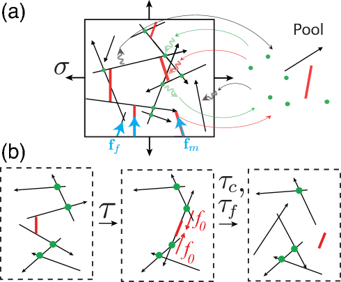
Figure 1: (a) Schematic illustration of a 2D cytoskeletal network (left). Filaments are represented by black arrows, motors by red bars and cross linkers by green dots. The network exerts a stress $\sigma$ on the boundaries of the box, arising from tensions acting within the filaments ($\mathbf{f}_{f}$) and within the motors ($\mathbf{f}_{m}$). Motors move towards the arrowhead of filaments (for actin, the arrowhead corresponds to the barbed end). Network components stochastically exchange with a reservoir (right). (b) Motors move on filaments and rearrange the network on a timescale $\tau$. Crosslinkers and actin filaments turn over on longer timescales $\tau_{c}>\tau$ and $\tau_{f}>\tau$.

To obtain forces acting on filaments, we introduce the effective mechanical potential, $U=W+{\bm{\lambda}}\cdot{\bm{g}}({\bm{x}}_{f,i},{\bm{n}}_{f,i},{\bm{x}}_{m,k},{\bm{n}}_{m,k})$, where $W=-f_{0}\sum_{\langle k,i\rangle}s_{ki}$ is the work due to motor active forces, with $s_{ki}$ the position of the $k$-th motor head on the $i$-th filament relative to the filament centre of mass, and the sum $\sum_{\langle k,i\rangle}$ is performed for all the pairs of filaments ($i$) and motors ($k$) connected with each other. In addition, geometrical constraints arise from the conditions that cross linkers and motor heads are firmly attached to filaments, and that motor filaments have a fixed length. The coefficients ${\bm{\lambda}}$ are Lagrange multipliers imposing these constraints, ${\bm{g}}({\bm{x}}_{f,i},{\bm{n}}_{f,i},{\bm{x}}_{m,k},{\bm{n}}_{m,k})={\bm{0}}$, where ${\bm{x}}_{f,i}$ and ${\bm{n}}_{f,i}$ (resp. ${\bm{x}}_{m,k}$, ${\bm{n}}_{m,k}$) indicate the centre of mass position and orientation unit vector of the $i$-th filament (resp. $k$-th motor). The motion of motors is taken into account by writing that the position of attachment of the $k$-th motor $s_{ki}$ relative to the centre of mass of the filament $i$ follows the dynamic equation

$$\mu\frac{ds_{ki}}{dt}=-\frac{\partial U}{\partial s_{ki}}$$ (1)

with $\mu$ a scalar friction coefficient arising from translational friction between the motor heads and the filament Tawada91 ; Imafuku99 ; Julicher:1995mb . Motors have a typical velocity $v_{m}=f_{0}/\mu$, and we introduce a reference timescale $\tau=l_{f}\mu/(2f_{0})$. We neglect viscous forces arising from the fluid around the network compared to motor-filament friction, and the position and orientation of filaments $\mathbf{x}_{f,i}$, $\mathbf{n}_{f,i}$ are relaxed instantaneously.

To fix ideas, cortical actomyosin networks in a cell have a mesh size $\xi\sim 20-250$nm Morone:2006uq ; Charras:2006yq and the typical cell diameter is several tens of micrometers. We therefore expect actin filaments to have a length $l_{f}$ of order $0.1-1\mu$m, smaller than their persistence length $l_{p}=16\mu$m ott1993measurement . Myosins move on actin filaments with velocity $v_{m}\sim 0.1-3\mu$m/s ishikawa2003polarized ; kubalek1992dictyostelium . The characteristic time for the myosins to move on a filament is $\tau\sim l_{f}/v_{m}\sim 0.03-10$s. To compare this timescale to the effect of viscous stresses arising in the solvent of viscosity $\eta$, we note that the velocity of a filament in the network subjected to a force $f_{0}$ is $\sim f_{0}\ln(\xi/r_{f})/(\eta l_{f})$, giving a timescale $\tau_{v}\sim l_{f}^{2}\eta/(f_{0}\ln(\xi/r_{f}))$, with $r_{f}\simeq 5nm$ the radius of a filament. Taking the force exerted by a myosin $f_{0}\sim 6-12pN$, $\eta\simeq 10^{-3}Pa.s$ for water, we find $\tau_{v}\sim 10^{-4}$s $\ll\tau$. Finally, we expect the characteristic times $\tau_{c}$ and $\tau_{f}$ of the crosslinker and actin filament turnover, respectively, to be of the order of $10$ s- $1$ min Mukhina:2007ve ; Reichl:2008fr , slow compared to these timescales, such that $\tau_{c}\gg\tau$ and $\tau_{f}\gg\tau$.

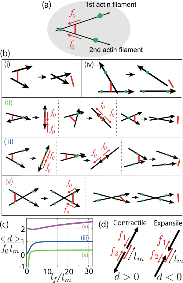
Figure 2: Contractile and expansile configurations for one motor and two filaments. (a) Two filaments are attached by fixed cross linkers to the external network. (b) (Left) Possible initial configurations for one motor, two filaments and one or several cross linkers, and final configurations. (c) Average strength of the contractile force dipole generated by the molecular motor $\langle d\rangle$ in the final configurations (ii), (iii), (v) where the motor does not detach, as a function of the filament length $l_{f}$. (d) Contractile (force dipole $d>0$) and expansile ($d<0$) configurations.

Configuration with one motor and two filaments.

We start by discussing the dynamics of configurations involving one motor attached to two filaments (Fig. 2a). The two filaments can be connected to a crosslinker, itself connected to the external network, which we consider here to be fixed in space. We distinguish several basic possible configurations, depending on the number and positions of attached passive crosslinkers (Fig. 2b): both filaments can be completely free (i), the two filaments can be crosslinked to each other (ii), or they can be crosslinked to the external network (iii)-(v).

To investigate how molecular motors modify the filaments organisation, we study the relaxation to final state of these different configurations. By averaging over possible initial configurations, we evaluate whether motors form on average positive or negative force dipoles in the network (Fig. 2c). The motor force dipole is $d=-(l_{m}/2)\mathbf{n}\cdot(\mathbf{f}_{1}-\mathbf{f}_{2})$, with $\mathbf{n}$ the unit vector giving the motor orientation, and $\mathbf{f}_{1}$ and $\mathbf{f}_{2}$ are the forces by which the motors pull or push the filaments (Fig. 2d). In case (v), $\mathbf{f}_{1}$ and $\mathbf{f}_{2}$ include not only the forces exerted by the motor themselves but also the forces originating from the geometrical constraint (Appendix A). We find that possible initial configurations can be classified in 2 categories (Fig. 2b). In cases (i) and (iv), filaments are moved relative to each other until the motor detaches, so that a motor-induced force dipole acts on a transient time $\tau$. This force dipole is expansile on average. In the quasi-static limit where $\tau\ll\tau_{c}$, the contribution of transient filament-motor configuration to the overall stress is negligible compared to steady motor configurations. When filaments either (ii) have only one fixed attachment point to the external network, (iii) are connected to each other by a cross linker, or (v) have both more than 2 cross linkers, they relax to a steady configuration where the motor exerts a constant force dipole. By averaging the resulting force dipole over possible initial configurations of the two filaments and the motor (Appendix A), we find that the motor exerts a contractile force dipole on average in cases (iii) and (v) (Fig. 2c). As in Ref. Dasanayake11 , the bias towards contractile states arises from instabilities of expansile configurations (Appendix A). The average force dipole $\langle d\rangle$ vanishes for point-like motors, $l_{m}\rightarrow 0$ lenz2014geometrical .

Numerical simulations of networks with turnover.

We next numerically simulated a network of $N_{f}$ filaments, $N_{m}$ motor rods and $N_{c}$ passive crosslinkers in a square box of width $W$ with periodic boundaries (Fig. 1). The frame of the box is not allowed to deform. We fixed the normalised motor density $l_{m}^{2}c$ to 1, where $c=N_{m}/W^{2}$ is the motor density. To make numerical simulations easier, the geometrical constraints ${\bm{g}}$ were replaced by linear springs mimicking the contacts at the junctions between motors and filaments, and at crosslinking points. Initial conditions are obtained by randomly positioning filaments in the network, and timescales are normalized to the reference time $\tau$. Turnover is introduced by stochastically removing cross linkers, motors and filaments from the network with rates $1/\tau_{c}$, $1/\tau_{m}$ and $1/\tau_{f}$. For simplicity, turnover rates of crosslinkers are taken here independent of the forces they sustain alvarado2013molecular . Filaments, motors and passive crosslinkers are added in the network with on-rates $k_{on}^{f}$, $k_{on}^{m}$ and $k_{on}^{c}$. New filaments take random positions and random orientation, motors take a randomly chosen position on two filaments points separated by a distance $l_{m}$, and passive crosslinkers are put on a randomly chosen filament intersection.

We evaluate the components of the stress tensor $\sigma_{ij}$ ($i,j=x\text{ or }y$) acting on the boundary of the box (Fig. 1a). The total stress is given by two contributions $\sigma_{ij}=\sigma_{ij}^{f}+\sigma_{ij}^{m}$, with $\sigma_{ij}^{f}$ obtained by summing forces acting both within the filaments and $\sigma_{ij}^{m}$ from forces acting within motor rods crossing the boundary of the box (Fig. 1). In a linear elastic or viscous material, $\sigma_{ij}^{f}=0$ in the absence of large-scale deformation. In a non-linearly elastic material however, $\sigma_{ij}^{f}\neq 0$ (Appendix B). At steady state, the average stress acting within the motors is given by (Ref. aditi2002hydrodynamic and Appedix B)

$$\sigma^{m}_{ij} \simeq \langle dn_{i}n_{j}c\rangle\ ,$$ (2)

where $\mathbf{n}$, $d$ and $c$ denote the orientation, motor-induced force dipole strength and concentration of bound motors. When the dipoles are isotropically oriented, $\sigma^{m}_{ij}=\sigma^{m}\delta_{ij}$ with $\sigma^{m}\simeq\langle dc\rangle/2$.

We first performed simulations without turnover of filaments. We focus on the isotropic component of the stress $\sigma\equiv(\sigma_{xx}+\sigma_{yy})/2$. Figure 3a (blue curve) shows the typical time evolution of the stress, for permanent crosslinkers and for crosslinkers with a finite lifetime. Without crosslinker turnover, the system reaches a stationary state where the stress $\sigma$ fluctuates around a finite positive value. Figure 3b shows the average value of the resulting stress (circles) as a function of the number of cross linkers $N_{c}$. For a small number of crosslinkers ($N_{c}\rightarrow 0$), no stress is observed, $\sigma=0$. Above a critical value of the number of crosslinkers $N_{c}>N_{c}^{*}\simeq N_{f}$, a transition occurs and a positive contractile stress appears in the system. When $N_{c}\sim N_{c}^{*}$ but $N_{c}<N_{c}^{*}$, although a portion of motors generate contractile force dipoles, filaments aggregate in clusters and hence $\sigma\sim 0$, suggesting that the transition is associated to the network connectivity (Supp movies M1 and M2). The stress then further increases with the number of crosslinkers and eventually saturates to a positive value. Such a transition to contractility as a function of the number of crosslinkers has been reported in in vitro reconstituted networks Bendix08 ; Koehler12 , as well as network clustering kohler2011structure .

The average stress only within the motors $\sigma^{m}$ is also plotted in Fig. 3b (cross marks). A similar transition occurs for a critical value of the number of cross linkers. The stress $\sigma^{m}$ is however larger than the total stress for a large number of cross linker $N_{c}>N_{f}$, implying that the filament network is under compression ($\sigma^{f}<0$). For large $N_{c}$, configurations (v) dominate in the network (Fig. 3c). The saturating value of $\sigma^{m}/\sigma_{0}\sim 0.6$ is nevertheless smaller than the average force dipole obtained by averaging all possible filament orientations $\langle d/2\rangle/(f_{0}l_{m})\sim 1.0$ (Fig. 2c); this is because some configurations do not relax to equilibrium on the characteristic timescale of myosin turnover.

Figure 3: Stress in a network of motors and filaments, with and without crosslinker turnover. (a) Time evolution of the normalised stress $\sigma/\sigma_{0}$ for $\tau_{c}^{-1}=0$, $N_{c}=1.2N_{f}$ (blue), $\tau_{c}=100\tau$, $N_{c}=1.6N_{f}$ (red) and $\tau_{c}=100\tau$, $N_{c}=1.2N_{f}$ (green). ($\sigma_{0}=f_{0}l_{m}N_{m}/W^{2}$) (b) Steady-state isotropic stress $\sigma$ (circles) and motor stress $\sigma^{m}$ (cross marks) as a function of the crosslinkers number $N_{c}$ for $\tau_{c}^{-1}=0$. (c) Fraction of different configurations (i)-(v) in Fig. 2 at steady state as a function of the crosslinker number $N_{c}$ for $\tau_{c}^{-1}=0$. (d) Isotropic stress $\sigma$ as a function of the crosslinker number $N_{c}$, for finite crosslinker lifetime $\tau_{c}=100\tau$, and for several simulation times ($\tau_{\rm sim.}=300,600,1,200$ and $2,400\tau$). Stress within the motors $\sigma_{m}$ is shown in the inset for $\tau_{\rm sim.}=300$ and $2,400\tau$. (e) Snapshots of a simulated network with crosslinker turnover ($N_{c}=1.2N_{f}$, $\tau_{c}=100\tau$). (f) Stress decay time $\tau_{\rm st}$ as a function of the crosslinker number $N_{c}$ with crosslinker turnover ($\tau_{c}=100\tau$). Solid line, theoretical prediction (see main text). Other parameters: $N_{f}=1,000$, $N_{m}=100$, $\tau_{f}^{-1}=0$, $k_{on}^{c}\tau_{c}=20$, $l_{f}=2l_{m}$, $W=10l_{m}$, $\tau_{m}=100\tau$ and $k_{on}^{m}\tau=20$.

When crosslinkers are allowed to turn over, the average stress first reaches a positive value before decaying to zero (Fig. 3a, red and green curves), even though the stress within the motors $\sigma^{m}$ is still non zero (Fig. 3d). The decay of the stress correlates with the collapse of the network in an isolated cluster, where filaments accumulate (Fig. 3e, Supp movie M3). To evaluate the decay timescale $\tau_{st}$, we fitted an exponentially decreasing function $\sigma(t)=A\exp(-t/\tau_{st})$ to the simulation results with fitting parameters $A$ and $\tau_{st}$. The decay timescale of the stress increases exponentially with $N_{c}$ for large $N_{c}$ (Fig. 3f). The relaxation timescale of the stress can be understood as follows: the timescale $\tau_{st}$ corresponds to the relaxation Maxwell time on which the network becomes fluid, due to turnover of passive crosslinkers enabling network rearrangements. This time can be estimated by

$$\tau_{st}=\frac{\tau_{c}}{n_{c}^{*}}(e^{n_{c}^{*}}-1)$$ (3)

with $n_{c}^{*}=2N_{c}/N_{f}$. To obtain Eq. (3), we assume that filaments with at least one crosslinker are fixed, and only filaments with no crosslinker attachment can rearrange. We then compute the first passage time at which a filament is free from cross linkers, starting from a configuration where the filament is attached with only one crosslinker (Appendix C). Equation (3) accounts for the characteristic time of stress decay in the network for large values of $N_{c}/N_{f}$ (Fig. 3f).

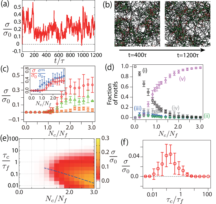
Figure 4: Stress in a network with filament turnover. (a) Time evolution of the stress in a network with crosslinkers and filament turning-over for $\tau_{f}=100\tau$, $\tau_{c}=100\tau$ and $N_{c}/N_{f}=1.6$. (b) Snapshots of the network evolution corresponding to (a). (c) Steady-state stress $\sigma$ as a function of the number of crosslinkers for $\tau_{c}=\tau_{f}=100\tau$ (circles), $\tau_{c}=\tau_{f}=10\tau$ (triangles) and $\tau_{c}=\tau_{f}=1\tau$ (squares). Inset: steady-state stress $\sigma$ (circles) and motor stress $\sigma^{m}$ (cross marks) for $\tau_{c}=\tau_{f}=100\tau$. (d) Fraction of different configurations (i)-(v) at steady state, as a function of $N_{c}$ ($\tau_{c}=100\tau$, $\tau_{f}=100\tau$). (e) Heat map for contractile stress $\sigma$ as a function of $N_{c}$ and $\tau_{c}/\tau_{f}$ ($\tau_{c}=\tau$). The broken line indicates $\tau_{f}=\tau_{\rm st}$. (f) Stress as a function of the ratio of filament and crosslinker turnover rate ($\tau_{c}=\tau$, $N_{c}=1.6N_{f}$). Other parameters as in Fig. 3, except $\tau_{m}^{-1}=0$.

We now turn to simulations where both filaments and crosslinkers turn over. In the cell, actin filaments polymerise and depolymerise. Here, we account for this process by simply introducing a rate of filament turnover, $\tau_{f}^{-1}$. Passive crosslinkers and motor heads are removed together with the filaments to which they are attached. Remarkably, with both crosslinker and filament turnover, the network evolves towards a steady state with a non-zero positive stress (Fig. 4a-b). As in the previous case, a transition from a non-contractile to a contractile network appears when the number of crosslinkers $N_{c}$ is increased (Fig. 4c, Supp movies M4 and M5). Note that the stress $\sigma$ deviates again from the average stress within the motors $\sigma^{m}$ (Fig. 4c, inset). The dependency of the fraction of configurations as a function of $N_{c}$ is qualitatively similar to the case without filament turnover (Fig. 4d).

We then varied the filament turnover timescale $\tau_{f}$ (Fig. 4c,e,f). We find that the stress reaches a maximum for intermediate values of the filament turnover timescale (broken line in Fig. 4e, and Fig. 4f): for slow filament turnover $\tau_{f}\gg\tau_{\rm st}$, the network collapses in clusters due to crosslinker turnover, while for fast filament turnover $\tau_{f}\ll\tau_{\rm st}$, filaments are removed before motors reach a configuration where they can exert a force dipole in the network. We find that the optimum value of the ratio of turnover time scale in Fig. 4f, $\tau_{f}/\tau_{c}\sim 10$, is of the order of the ratio experimentally measured values of turn-over of actin and crosslinker in the cell cortex, $\tau_{f}\sim 15-45$s and $\tau_{c}\sim 7-14$s Guillaume12 .

Conclusion.

We propose the following dynamic picture for the stress generated in a rearranging network: molecular motors move on filaments on a timescale $\tau$, fast compared to the crosslinker turnover $\tau_{c}$. When molecular motors bind to pairs of filaments, they either displace them and detach, or find steady configurations where they generate predominantly contractile force dipoles (Figs. 2 and 3a-c). In networks with permanent crosslinkers, a transition to contractile state of the network occurs for a large enough number of crosslinkers (Fig. 3b). When crosslinkers are allowed to turnover, the network can rearrange and flow, filaments collapse in a cluster, and the total stress in the network vanishes even though the stress only within the motors is still contractile (Fig. 3a,d-f). Introducing filament turnover occurring on a timescale $\tau_{f}$ comparable to the crosslinker turnover timescale $\tau_{c}$ prevents this clustering mechanism, and allows the network to generate a steady-state contractile stress (Fig. 4). It will be interesting to investigate stress generation in in vitro experiments where crosslinkers and filaments are allowed to turn over.

Acknowledgements: We thank Matthew Smith for helpful discussions. This work was supported partly by the JSPS Institutional Program for Young Researcher Overseas Visits (T.H.), the Postdoctoral Research Fellowship of the Alexander von Humboldt foundation (T.H.), the JSPS Core-to-Core Program (T.H.), the Max Planck Gesellschaft (G.S.), and the Francis Crick Institute which receives its core funding from Cancer Research UK, the UK Medical Research Council, and the Wellcome Trust (G.S).

Appendix A Calculation of the average force dipole for two filaments

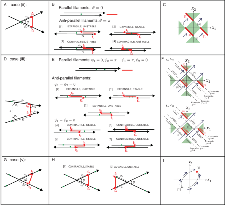
Figure 5: Final configurations reached by two filaments bound by a motor, with the filaments attached to a rigid external network with a varying number of cross linkers. A, D, G, example configurations for each case, according to the number of cross linkers; B, E, H, corresponding possible steady-state configurations; C,F,I, Phase plot of the dynamics of the motor according to the coordinates of its position on the two filaments, $x_{1}$, $x_{2}$. Red lines and dots correspond to stable steady-state configurations, while dotted black lines correspond to unstable steady-state configurations. Green regions represent values of the coordinates $x_{1}$ and $x_{2}$ which are not geometrically accessible.

We detail here how we obtain the average force dipole exerted by a motor on two filaments in the configurations shown in Fig. 2. As mentioned in the text, we assume here that crosslinkers are rigidly fixed to the external network. The geometry of the two filaments and motor can be described the position of the motors on the two filaments $s_{1}$, $s_{2}$ and by the two angles $\psi_{i}$ between the motor filament and $i$-th filament ($i=1,2$). The motor positions $s_{i}$ evolve according to

$$\mu\frac{ds_{i}}{dt}=-\frac{\partial U}{\partial s_{i}},$$ (4)

while the angles $\psi_{i}$ relax instantaneously, so that $\partial U/\partial\psi_{i}=0$.

A.1 No crosslinkers attached, or one filament is attached by only one crosslinker and the other filament is rigidly attached to the external network

Case (i) and (iv): In these situations, no steady-state is reached as the motor always unbinds from the two filaments.

A.2 Two filaments attached to each other by a crosslinker

Case (ii): When the two filaments are attached by a single crosslinker, the mechanical potential $U$ reads

$$U=-f_{0}(x_{1}+x_{2})+\lambda\left(\sqrt{x_{1}^{2}+x_{2}^{2}-2x_{1}x_{2}\cos\theta}-l_{m}\right)$$ (5)

with $x_{1}$ and $x_{2}$ the distances between the myosin attachment points to the crossing point of the two filaments, taken positive in the direction of the filament towards which motors move (Fig. 5A). $\theta$ is the angle between the two filaments, such that $\mathbf{n}_{1}.\mathbf{n}_{2}=\cos\theta$, with $\mathbf{n}_{i}$ the unit vector giving the orientation of the filament $i$. In addition, $\lambda$ is a Lagrange multiplier ensuring that the length $l_{m}$ of the motor is fixed. Three situations can then occur:

• when $\theta\neq 0$ and $\theta\neq\pi$ and the filaments are not parallel neither antiparallel, the angle $\theta$ is given by

  $$\cos\theta=\frac{x_{1}^{2}+x_{2}^{2}-l_{m}^{2}}{2x_{1}x_{2}}$$ (6)

  and is free to adjust as the motor position changes. The evolution of the position of the motor on the filaments is given by

  $$\mu\frac{dx_{1}}{dt} = f_{0}$$ (7)

  $$\mu\frac{dx_{2}}{dt} = f_{0}$$ (8)

  such that the motor moves until it detaches from the filaments, or until the filaments become parallel or antiparallel.

• When the two filaments are parallel and point in the same direction, $\theta=0$ and $(x_{1}-x_{2})^{2}=l_{m}^{2}$. The center of mass of the motor at position $(x_{1}+x_{2})/2$ follows the dynamic equation

  $$\mu\frac{d}{dt}\frac{x_{1}+x_{2}}{2}=f_{0}$$ (9)

  and the motor moves on the filament until it detaches.

• When the two filaments are antiparallel, $\theta=\pi$ and $(x_{1}+x_{2})^{2}=l_{m}^{2}$. Two configurations are then possible, according to whether the two filaments point away or towards the center of the motor from their attachment point to the motor. These two configurations correspond respectively to $x_{1}+x_{2}=-l_{m}$ (expansile configuration) and $x_{1}+x_{2}=l_{m}$ (contractile configuration). Any position of the motor on the filament is then a steady-state solution, as long as the two motor ends each bind on the filaments.

  To test for the stability of these two configurations, we consider a slight change of the angle between the two filaments, $\theta=\pi+\delta\theta$, with $|\delta\theta|\ll 1$. We take the initial position of the motor to be $x_{1}=x_{0}+\chi l_{m}/2$ and $x_{2}=-x_{0}+\chi l_{m}/2$, with $\chi=-1$ for an expansile configuration and $\chi=1$ for a contractile configuration. $x_{0}=(x_{1}-x_{2})/2$ is the position of the center of mass of the motor, relative to the crosslinker joining the two filaments, measured positively in the direction of the first filament. We find then the following dynamic equation for $\delta\theta$:

  $$\mu\frac{d\delta\theta}{dt} = \frac{dx_{1}}{dt}\frac{\partial\theta}{\partial x_{1}}+\frac{dx_{2}}{dt}\frac{\partial\theta}{\partial x_{2}}$$ (10)

  $$= f_{0}\frac{8\chi l_{m}}{l_{m}^{2}-4x_{0}^{2}}\frac{1}{\delta\theta}$$

  where we have used Eqs. (6), (7) and (8) from the first to the second line. The sign of the right hand side of Eq. (10) indicates whether the angle $\theta$ increases or decreases when the two filaments are slightly rotated away from their antiparallel configuration. Therefore, the associated configuration is unstable when the sign is positive, and stable otherwise. We find therefore that the stability of the configuration depends on the position of the center of mass of the motor: for $|x_{0}|<l_{m}/2$ (motor near the crosslinker), the expansile configuration is stable, and the contractile configuration unstable. For $|x_{0}|>l_{m}/2$ (motor away from the cross-linker), the expansile configuration is unstable and the contractile configuration is stable.

The flow diagram in Fig. 5C case (ii) shows the corresponding dynamics in the space of the motor position $(x_{1},x_{2})$. Red segments indicate the stable steady states. In the green regions, no value of the angle $\theta$ allows for the motor to have position ($x_{1}$, $x_{2}$) on the two filaments.

A.3 Two filaments, each attached by a crosslinker to the external network

The mechanical potential reads in that case

$$U=-f_{0}(x_{1}+x_{2})+\lambda\left[\sqrt{x_{1}^{2}+x_{2}^{2}+l_{m}^{2}+2x_{1}l_{m}\cos\psi_{1}+2x_{2}l_{m}\cos\psi_{2}+2x_{1}x_{2}\cos(\psi_{1}+\psi_{2})}-a\right],$$ (11)

with $x_{1}$ and $x_{2}$ the distances between the myosin attachment point and the crosslinker position on each filament, and $a$ the distance between the two cross linkers (Fig. 5D). $\lambda$ is a Lagrange multiplier imposing that the length of the motor is equal to $l_{m}$. In this subsection, we use for convenience the dynamics of the angle between motor and filaments $\psi_{1}$ and $\psi_{2}$ to characterise the orientation of the filaments. The dynamics in the limit where $\psi_{1}$ and $\psi_{2}$ relax quasi statically is given by

$$\mu\frac{\partial x_{1}}{\partial t} = f_{0}+\frac{\lambda}{a}\left(x_{1}+l_{m}\cos\psi_{1}+x_{2}\cos(\psi_{1}+\psi_{2})\right)$$ (12)

$$\mu\frac{\partial x_{2}}{\partial t} = f_{0}+\frac{\lambda}{a}\left(x_{2}+l_{m}\cos\psi_{2}+x_{1}\cos(\psi_{1}+\psi_{2})\right)$$ (13)

$$\epsilon\mu a^{2}\frac{\partial\psi_{1}}{\partial t} = -\frac{\lambda}{a}\left(x_{1}l_{m}\sin\psi_{1}+x_{1}x_{2}\sin(\psi_{1}+\psi_{2})\right)$$ (14)

$$\epsilon\mu a^{2}\frac{\partial\psi_{2}}{\partial t} = -\frac{\lambda}{a}\left(x_{2}l_{m}\sin\psi_{2}+x_{1}x_{2}\sin(\psi_{1}+\psi_{2})\right)$$ (15)

where $\epsilon\ll 1$ is a factor that vanishes in the quasi-static limit where the filaments rotate adiabatically. Solving for the Lagrange multiplier $\lambda$ by imposing the constraint that the length of the motor is equal to $l_{m}$, we obtain:

$$\lambda = -\epsilon f_{0}a^{3}\frac{(x_{1}+x_{2})(1+\cos(\psi_{1}+\psi_{2}))+l_{m}(\cos\psi_{1}+\cos\psi_{2})}{A+B\epsilon a^{2}}$$ (16)

$$A = (x_{1}l_{m}\sin\psi_{1}+x_{1}x_{2}\sin(\psi_{1}+\psi_{2}))^{2}+(x_{2}l_{m}\sin\psi_{2}+x_{1}x_{2}\sin(\psi_{1}+\psi_{2}))^{2}$$

$$B = \left(x_{1}+l_{m}\cos\psi_{1}+x_{2}\cos(\psi_{1}+\psi_{2})\right)^{2}+\left(x_{2}+l_{m}\cos\psi_{2}+x_{1}\cos(\psi_{1}+\psi_{2})\right)^{2}$$

where the coefficient $A$ vanishes when the filaments are aligned with the motor. Several situations can again be distinguished:

• When the filaments are neither parallel nor antiparallel, from Eq. (16), $\lambda\sim\epsilon$ in the limit $\epsilon\rightarrow 0$. Eqs. (12) and (13) then yield at the lowest order in $\epsilon$

  $$\mu\frac{dx_{1}}{dt} = f_{0}+O(\epsilon)$$ (17)

  $$\mu\frac{dx_{2}}{dt} = f_{0}+O(\epsilon)$$ (18)

  such that no steady-state exists in that situation.

• When the filaments are parallel and point in the same direction, $(\psi_{1},\psi_{2})=(0,\pi)$ or $(\psi_{1},\psi_{2})=(\pi,0)$. In that case $\lambda=0$ and no steady-state exists for the motor, which runs on the two filaments before detachment.

• When the filaments are antiparallel, $(\psi_{1},\psi_{2})=(0,0)$ (expansile configuration) or $(\psi_{1},\psi_{2})=(\pi,\pi)$ (contractile configuration). In the expansile configuration, $x_{1}+x_{2}+l_{m}=\chi a$, with $\chi=\pm 1$. In the contractile configuration, $x_{1}+x_{2}-l_{m}=\chi a$, with the same rule applying for $\chi$. In both cases, Eq. (16) yields $\lambda=-\chi f_{0}$ and any position of the motor is a steady-state.

  To test for the stability of these steady states, we consider the dynamics of $\psi_{1}$ and $\psi_{2}$ around $\psi_{1}=\psi_{2}=\psi^{*}$ with $\psi^{*}\equiv 0$ or $\pi$, $\psi_{1}=\psi^{*}+\delta\psi_{1}$ and $\psi_{2}=\psi^{*}+\delta\psi_{2}$. To regularise the dynamics around the parallel filaments state, we consider a situation with finite $\epsilon$ and consider perturbations verifying $\delta\psi\ll\sqrt{\epsilon}$, such that $\lambda\simeq-\chi f_{0}$. From Eqs. (14) and (15), we have then

  $$\epsilon\mu a\frac{d\delta\psi_{1}}{dt} = \frac{\chi f_{0}}{a}\left[(x_{1}l_{m}\cos\psi^{*}+x_{1}x_{2})\delta\psi_{1}+x_{1}x_{2}\delta\psi_{2}\right]$$ (19)

  $$\epsilon\mu a\frac{d\delta\psi_{2}}{dt} = \frac{\chi f_{0}}{a}\left[x_{1}x_{2}\delta\psi_{1}+(x_{2}l_{m}\cos\psi^{*}+x_{1}x_{2})\delta\psi_{2}\right]\ ,$$ (20)

  so that the state $\psi_{1}=\psi_{2}=\psi^{*}$ is stable if $\chi(x_{1}l_{m}\cos\psi^{*}+x_{2}l_{m}\cos\psi^{*}+2x_{1}x_{2})<0$ and $(x_{1}l_{m}\cos\psi^{*}+x_{1}x_{2})(x_{2}l_{m}\cos\psi^{*}+x_{1}x_{2})-x_{1}^{2}x_{2}^{2}>0$, whereas it is unstable otherwise. Taking the initial condition to be $x_{1}=x_{0}/2+(\chi a-l_{m}\cos\psi^{*})/2$ and $x_{2}=-x_{0}/2+(\chi a-l_{m}\cos\psi^{*})/2$ at the steady state, the stability condition is satisfied when

  $$\chi(x_{0}^{2}+l_{m}^{2}-a^{2})>0\text{ and }x_{1}x_{2}\chi\cos\psi^{*}>0\ .$$ (21)

The results are summarized in the flow diagram in Fig. 5F. Red segments indicate the stable steady states. In the green region, there are no possible values of $\psi_{1}$ and $\psi_{2}$ for given values of $x_{1}$ and $x_{2}$.

A.4 Two filaments rigidly attached to the external network

This situation corresponds to case (v). The mechanical potential $U$ reads as for case (ii)

$$U=-f_{0}(x_{1}+x_{2})+\lambda\left(\sqrt{x_{1}^{2}+x_{2}^{2}-2x_{1}x_{2}\cos\theta}-l_{m}\right),$$ (22)

with $x_{1}$ and $x_{2}$ the distances to the crossing point of the two filaments, taken positive in the direction of the filament towards which motors move (Fig. 5G). $\theta$ is the angle between the two filaments, such that $\mathbf{n}_{1}.\mathbf{n}_{2}=\cos\theta$, with $\mathbf{n}_{i}$ the unit vector giving the orientation of the filament $i$. $\lambda$ is a Lagrange multiplier ensuring that the length $l_{m}$ of the motor is fixed. The dynamic equation for the motion of the motor on the two filaments Eq. (4) then reads

$$\mu\frac{\partial x_{1}}{\partial t} = f_{0}-\frac{\lambda}{l_{m}}(x_{1}-x_{2}\cos\theta)$$ (23)

$$\mu\frac{\partial x_{2}}{\partial t} = f_{0}-\frac{\lambda}{l_{m}}(x_{2}-x_{1}\cos\theta),$$ (24)

where $\theta$ is a fixed angle, and the Lagrange multiplier $\lambda$ is obtained from the constraint that $x_{1}^{2}+x_{2}^{2}-2x_{1}x_{2}\cos\theta=l_{m}^{2}$:

$$\lambda=\frac{f_{0}l_{m}(x_{1}+x_{2})(1-\cos\theta)}{(x_{1}-x_{2}\cos\theta)^{2}+(x_{2}-x_{1}\cos\theta)^{2}}$$ (25)

Two solutions can be found for the motor position on the two filament, assuming that they are not parallel ($\theta\neq 0$ and $\theta\neq\pi$):

$$x_{1}=x_{2}=\pm\frac{l_{m}}{2\sin\frac{\theta}{2}}$$ (26)

As pointed out in Ref. Dasanayake11 , a linear stability analysis around the steady-state indicates that only the positive solutions $x_{1}=x_{2}=l_{m}/[2\sin(\theta/2)]$ is stable. The corresponding force dipole at equilibrium is positive and is given by

$$d=\frac{l_{m}f_{0}}{\sin(\frac{\theta}{2})}.$$ (27)

Therefore, the dipole formed on two rigidly fixed, non-parallel filaments is always contractile (Fig. 5H-I).

A.5 Averaging force dipole

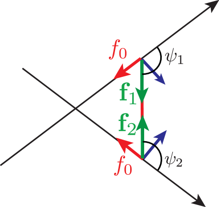
Figure 6: Schematic of the force dipole exerted by a motor. Each motor exerts a force of magnitude $f_{0}$ parallel to the filament. The total force exerted by the motor on the filament are equal and opposite at steady-state and denoted $f_{1}$ and $f_{2}$. The contribution of the force normal to the filament arises from geometrical constrains. Overall, this results in a tension $f=|\mathbf{f}_{1}|=|\mathbf{f}_{2}|$ acting within the motor, which is used here to define the force dipole exerted by a motor.

To obtain the associated average force dipole exerted by the motor in these different configurations, we proceed as follows: denoting as $\mathbf{c}_{12}^{(0)}$ the initial distance between the two filaments, $\theta_{f,1}^{(0)}$ and $\theta_{f,2}^{(0)}$ the two angles giving the initial orientations of the filaments, $x_{f,1}^{(0)}$, $x_{f,2}^{(0)}$ the initial position of the two motors on the filaments, and $r_{k}$ ($k=1,\cdots,N_{c}$ with $N_{c}$ the number of crosslinkers attached to the external network) the position of the crosslinkers on the filaments, we compute the motor-induced force dipole $d$ reached at steady-state as shown in Fig. 5; cases (ii), (iii) and (v) by

$$d(\mathbf{c}_{12}^{(0)},\theta_{f,1}^{(0)},\theta_{f,2}^{(0)},x_{1}^{(0)},x_{2}^{(0)},\{r_{k}\}_{k})=\frac{l_{m}f_{0}}{2\cos\psi_{1}}+\frac{l_{m}f_{0}}{2\cos\psi_{2}}\ ,$$ (28)

where the angles $\psi_{1}$ and $\psi_{2}$ between the motor and two filaments at steady-state are functions of $\mathbf{c}_{12}^{(0)}$, $\theta_{f,1}^{(0)}$, $\theta_{f,2}^{(0)}$, $x_{1}^{(0)}$, $x_{2}^{(0)}$ and $\{r_{k}\}_{k}$. Equation (28) is obtained from the definition of the force dipole

$$d=-\frac{l_{m}}{2}\mathbf{n}\cdot(\mathbf{f}_{1}-\mathbf{f}_{2})$$ (29)

with $\mathbf{n}$ the unit vector giving the motor orientation pointing towards filament 1, and $\mathbf{f}_{i}$ with $i=1,2$ are the forces exerted by the motor on the two filaments. The dependencies $1/\cos\psi_{i}$ ($i=1,2$) in Eq. (28) arise from the condition that the projections of the forces $\mathbf{f}_{i}$ on the filament $i$ have magnitude $f_{0}$ (Fig. 6).

The average force dipole is then obtained by

$$<d>=\int d\mathbf{c}_{12}^{(0)}\int_{0}^{2\pi}\frac{d\theta_{f,2}^{(0)}}{2\pi}\int_{0}^{2\pi}\frac{d\theta_{f,2}^{(0)}}{2\pi}\int\left(\prod_{k=1}^{N_{c}}\frac{dr_{k}}{L_{f}}\right)\int\frac{d(x_{1}^{(0)},x_{2}^{(0)})}{\Gamma}d(\mathbf{c}_{12}^{(0)},\theta_{f,1}^{(0)},\theta_{f,2}^{(0)},x_{1}^{(0)},x_{2}^{(0)},\{r_{k}\}_{k})\ ,$$ (30)

where the integration $\int d(x_{1}^{(0)},x_{2}^{(0)})$ runs for all possible initial motor configurations $x_{1}^{(0)}$, $x_{2}^{(0)}$ that eventually reach a steady state, and $\Gamma=\int d(x_{1}^{(0)},x_{2}^{(0)})1$.

Appendix B Relationship between the stress and the average force dipole

In this section, we discuss the two contributions to the stress generated by the filament and motor network, $\sigma_{ij}^{f}$ and $\sigma_{ij}^{m}$. We point out that in the absence of large scale deformations, $\sigma_{ij}^{f}$ can contribute to the total stress, when the elastic response of the filament network is non-linear.

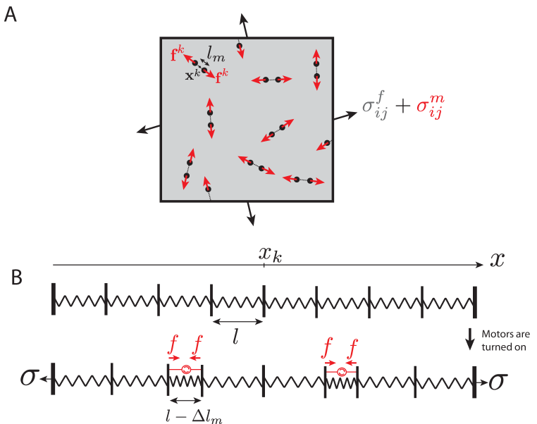
Figure 7: A. Schematic of a 2D elastic material, subjected to forces arising from force dipoles exerted by motor filaments. Motors result in a stress $\sigma_{ij}$ acting at the boundary of the box. B. Schematic of a 1D chain of non linear springs subjected to force dipoles. The chain contains $N$ springs and is fixed at both ends. Motors result in a force $\sigma$ along the chain.

B.1 Two-dimensional, linear elastic material

We consider here a two-dimensional elastic material subjected to the force dipoles exerted by motor filaments. The motor force dipoles consist of two opposite forces $\mathbf{f}^{k}=\pm f^{k}\mathbf{n}^{k}$, separated by a distance $l_{m}$, and where the index $k$ label the motors. The motors induce a deformation in the elastic material. The total stress in the system is then the sum of the resulting elastic stress, denoted $\sigma_{ij}^{f}$, and the stress generated within the motors, denoted $\sigma_{ij}^{m}$:

$$\sigma_{ij}=\sigma_{ij}^{f}+\sigma_{ij}^{m}$$ (31)

We start by discussing the average stress created by an ensemble of motors in a 2D material. Following Ref. aditi2002hydrodynamic , we now show that when the system is homogeneous, force balance on a section $\mathcal{S}$ of the network enclosed in a contour $\mathcal{C}$ allows to relate the stress generated within motors to the concentration and orientation of motors. To evaluate the stress, we first note that each motor $k$ corresponds to a line under tension $f^{k}$ with length $l_{m}$, orientation $\mathbf{n}^{k}$, centered at position $\mathbf{x}^{k}$, and joining the two points at coordinates $\mathbf{x}^{k}-l_{m}/2\mathbf{n}^{k}$ and $\mathbf{x}^{k}+l_{m}/2\mathbf{n}^{k}$ (Fig. 7A). Therefore, the two-dimensional stress field within the motors can be written

$$\sigma_{ij}^{m}(\mathbf{x})=\sum_{k}f^{k}n^{k}_{i}n^{k}_{j}\int_{-\frac{l_{m}}{2}}^{\frac{l_{m}}{2}}du\delta(\mathbf{x}-(\mathbf{x}^{k}+\mathbf{n}^{k}u))$$ (32)

where $u$ is a coordinate going along the line under tension $f^{k}$. The average stress within a region $\mathcal{S}$ of surface area $S$ is then given by

$$\langle\sigma_{ij}^{m}\rangle = \frac{1}{S}\int_{\mathcal{S}}d\mathbf{x}\sigma^{m}_{ij}(\mathbf{x})$$ (33)

$$= \frac{1}{S}\int_{\mathcal{S}}d\mathbf{x}\sum_{k}f^{k}n^{k}_{i}n^{k}_{j}\int_{-\frac{l_{m}}{2}}^{\frac{l_{m}}{2}}du\delta(\mathbf{x}-(\mathbf{x}^{k}+\mathbf{n}^{k}u))$$ (34)

$$= \frac{1}{S}\sum_{k}f^{k}l_{m}n_{i}^{k}n_{j}^{k}$$ (35)

$$= c\langle dn_{i}n_{j}\rangle$$ (36)

where $c$ is the concentration of motors, $d^{k}=l_{m}f^{k}$ is the dipole strength of motor $k$, and the averaging $\langle\cdot\rangle$ is performed over space.

In a linearly elastic material, the average stress within the network of filaments is given by

$$\sigma_{ij}^{f}=2E\left(u_{ij}-\frac{1}{2}u_{kk}\delta_{ij}\right)+Ku_{kk}\delta_{ij}$$ (37)

with $E$ and $K$ a shear and bulk elastic moduli, and $u_{ij}=\frac{1}{2}(\partial_{i}u_{j}+\partial_{j}u_{i})$ the gradient of deformation. The average stress generated in the elastic material in a region $\mathcal{S}$ with contour $\mathcal{C}$ and surface area $S$ is then given by

$$\langle\sigma_{ij}^{f}\rangle = \frac{1}{S}\int_{\mathcal{S}}d\mathbf{x}\sigma^{f}_{ij}$$ (38)

$$= \frac{2E}{S}\int_{\mathcal{S}}d\mathbf{x}u_{ij}+\frac{K-E}{S}\int_{\mathcal{S}}d\mathbf{x}u_{kk}\delta_{ij}$$ (39)

$$= \frac{E}{S}\int_{\mathcal{C}}dl\nu_{i}u_{j}+\frac{E}{S}\int_{\mathcal{C}}dl\nu_{j}u_{i}+\frac{K-E}{S}\int_{\mathcal{C}}dl\nu_{k}u_{k}\delta_{ij}$$ (40)

where $\boldsymbol{\nu}$ is the vector normal to the contour $\mathcal{C}$ and $dl$ an infinitesimal line element on the contour. If we consider a square box whose boundaries are fixed (Fig. 7A), or periodic boundary conditions, the contour integrals in Eq. (40) vanish. Therefore, for a linear elastic material with fixed boundaries, the average stress arises entirely from the forces acting within the motors. This however does not apply to a non-linearly elastic material, as we show in the next section.

B.2 One-dimensional chain of non-linear springs

We consider a simpler example in 1D of a periodic chain of $N$ elastic springs. Each spring is located between positions $x_{i}$ and $x_{i+1}$, with initial resting position $x_{i}=il$. The two points at the end of the chain, $x_{0}$ and $x_{N}$, are not allowed to move. In addition, $N_{m}$ motors are acting in parallel to a fraction $n=N_{m}/N$ of the springs (Fig. 7B). The motor exerts a constant force $f$. The springs have a non-linear force-extension relation

$$f_{e}=k\frac{\Delta l}{l}+k_{2}\left(\frac{\Delta l}{l}\right)^{2}$$ (41)

with $f_{e}$ the force exerted by the spring, $\Delta l=x_{i+1}-x_{i}-l$ the extension of the spring, and $k$ and $k_{2}$ are two spring constants. We assume that the springs are weakly non-linear, $k_{2}/k\ll 1$. In the initial resting position, $\Delta l=0$. The motors are then turned-on, driving a deformation of the the springs in the chain. The contraction of the springs which are in parallel with the motors is denoted $-\Delta l_{m}$. Because the overall length of the chain is kept fixed, the deformation of the free springs is then given by $\Delta l_{m}n/(1-n)$. We denote by $\sigma$ the total force acting within the chain. Force balance imposes that the total force within the springs and the motors is fixed and equal to $\sigma$, giving

$$\sigma = -k\frac{\Delta l_{m}}{l}+k_{2}\left(\frac{\Delta l_{m}}{l}\right)^{2}+f=k\frac{\Delta l_{m}}{l}\frac{n}{1-n}+k_{2}\left(\frac{\Delta l_{m}}{l}\frac{n}{1-n}\right)^{2}$$ (42)

where the second part of the equality is the total force within the springs in parallel with a motor, and the third part the force within the free springs. Solving these equations and expanding to first order in $fk_{2}/k^{2}\ll 1$, one obtains

$$\sigma=fn+\frac{k_{2}f^{2}n(1-n)}{k^{2}}$$ (43)

or using the concentration of motors $c=n/l$,

$$\sigma = flc+\frac{k_{2}f^{2}}{k^{2}}cl(1-cl)$$ (44)

$$= \sigma^{m}+\sigma^{f}$$ (45)

where $\sigma^{m}=flc$ is the average tension exerted within the motors. To leading order in the spring non linearity, $k_{2}\rightarrow 0$, the force within the chain reduces to the average motor tension $\sigma^{m}$, in agreement with Eq. (36). The non-linear elastic behaviour however brings a correction to this term $\sigma^{f}=k_{2}f^{2}cl(1-cl)/k^{2}$, proportional to the motor force squared, $f^{2}$.

Appendix C Network relaxation time

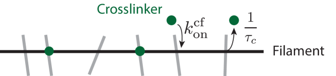
Figure 8: Schematic of a filament in the network. Crosslinkers bind to the filament with rate $k_{on}^{\rm{cf}}$ and unbind with rate $1/\tau_{c}$.

We derive here an approximate expression for the network characteristic relaxation time. We consider a filament within the network, crossing other filaments that are themselves immobilised. We expect this last assumption to be valid for a large enough number of crosslinkers. The number of crossing points is assumed to largely exceed the total number of crosslinkers in the network. Crosslinkers bind and unbind the filament at crossing points with other filaments. A filament with two attached crosslinkers is completely fixed, and can only rotate when it has one attached crosslinker. For simplicity we consider here that the filament can not rearrange to relax stresses unless no crosslinker attaches it to other filaments in the network. Once a filament is free, it can move until a crosslinker binds to it and immobilise it. We therefore estimate the network relaxation time as the mean first passage time to a state where no crosslinkers bind the filament, from a state where one crosslinker binds the filament.

We consider the probability of having $n_{c}$ crosslinkers on the filament, $P(n_{c})$. New crosslinkers bind to the filament with rate $k_{on}^{\rm{cf}}=2[k_{on}^{\rm{c}}/(1+k_{on}^{\rm{c}}\tau_{c})]N_{c}/N_{f}$, as crosslinkers bind to all filaments in the network with rate $k_{on}^{\rm{c}}$ (Fig. 8), and each crosslinker binds two filaments. In addition, crosslinkers unbind from the filament with rate $\tau_{c}^{-1}$ (Fig. 8). The probability $P(n_{c})$ then follows the master equation:

$$\frac{dP(n_{c})}{dt} =\frac{n_{c}+1}{\tau_{c}}P(n_{c}+1)+k_{on}^{\rm{cf}}P(n_{c}-1)-\left(\frac{n_{c}}{\tau_{c}}+k_{on}^{\rm{cf}}\right)P(n_{c})$$ (46)

Stationary distribution.

The stationary distribution of Eq. (46) is a Poisson distribution:

$$P(n_{c})=e^{-k_{on}^{\rm{cf}}\tau_{c}}\frac{(k_{on}^{\rm{cf}}\tau_{c})^{n_{c}}}{n_{c}!}$$ (47)

with mean and variance $n_{c}^{*}=k_{on}^{\rm{cf}}\tau_{c}\simeq 2N_{c}/N_{f}$ for $k_{on}^{\rm{c}}\tau_{c}\gg 1$.

Mean first passage time.

We now want to obtain the mean first passage time to reach a state where the filament has no bound crosslinker, $n_{c}=0$, starting from a configuration with $n$ crosslinkers attached on the filament. We denote $T_{n}$ this first passage time, and we follow a standard procedure to obtain its value gardiner1985stochastic ; pury2003mean . $T_{n}$ satisfies the following equation for $n>0$:

$$T_{n}=\frac{k_{on}^{\rm{cf}}}{k_{on}^{\rm{cf}}+n/\tau_{c}}T_{n+1}+\frac{n/\tau_{c}}{k_{on}^{\rm{cf}}+n/\tau_{c}}T_{n-1}+\frac{1}{k_{on}^{\rm{cf}}+n/\tau_{c}}$$ (48)

where the first term corresponds to the probability of moving to a state with $n+1$ bound crosslinkers, times the waiting time from the state $n+1$, the second term is the product of the probability to move to a state with $n-1$ bound crosslinkers times the waiting time from the state $n-1$, and the last term is the average time spent in the state $n$. In addition, $T_{0}=0$ by definition of the first passage time $T_{n}$, and we take a reflecting boundary condition at infinity, implying $T_{n}-T_{n-1}\rightarrow 0$ for $n\rightarrow\infty$. Equation (48) can be rewritten

$$k_{on}^{\rm{cf}}(T_{n}-T_{n+1})+\frac{n}{\tau_{c}}(T_{n}-T_{n-1})=1$$ (49)

or defining $z_{n}=T_{n+1}-T_{n}$,

$$z_{n}=\frac{n}{k_{on}^{\rm{cf}}\tau_{c}}z_{n-1}-\frac{1}{k_{on}^{\rm{cf}}}$$ (50)

To solve this equation, one introduces $Z_{n}=z_{n}(k_{on}^{\rm{cf}}\tau_{c})^{n}/n!$, which satisfies then:

$$Z_{n}=Z_{n-1}-\frac{(k_{on}^{\rm{cf}}\tau_{c})^{n}}{k_{on}^{\rm{cf}}n!}$$ (51)

Solving Eq. (51) then yields the following expression for $Z_{n}$, $z_{n}$ and $T_{n}$, using that $Z_{\infty}=0$:

$$Z_{n} = \sum_{k={n+1}}^{\infty}\frac{(k_{on}^{\rm{cf}}\tau_{c})^{k}}{k_{on}^{\rm{cf}}k!}$$ (52)

$$z_{n} = \frac{n!}{(k_{on}^{\rm{cf}}\tau_{c})^{n}}\sum_{k={n+1}}^{\infty}\frac{(k_{on}^{\rm{cf}}\tau_{c})^{k}}{k_{on}^{\rm{cf}}k!}$$ (53)

$$T_{n} = \sum_{k=0}^{n-1}\frac{k!}{(k_{on}^{\rm{cf}}\tau_{c})^{k}}\sum_{m={k+1}}^{\infty}\frac{(k_{on}^{\rm{cf}}\tau_{c})^{m}}{k_{on}^{\rm{cf}}m!}$$ (54)

From this last expression, one finally obtains $T_{1}$,

$$T_{1} = \sum_{m=1}^{\infty}\frac{(k_{on}^{\rm{cf}}\tau_{c})^{m}}{k_{on}^{\rm{cf}}m!}$$ (55)

$$= \frac{1}{k_{on}^{\rm{cf}}}(e^{k_{on}^{\rm{cf}}\tau_{c}}-1)$$ (56)

$$= \frac{\tau_{c}}{n_{c}^{*}}(e^{n_{c}^{*}}-1)$$ (57)

The time $T_{1}$ therefore contains a factor increasing exponentially with the number of crosslinkers per filament $n_{c}^{*}$. We use the time $T_{1}$ as an estimate for the network relaxation time. In Fig. 3f, we verify that the time $T_{1}$ provides a good approximation for the relaxation time of the network.

Appendix D Effect of motor concentration and dispersion in motor forces

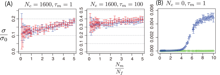
Figure 9: A. Isotropic stress as a function of the number of motors $N_{m}$, for two values of myosin turn-over. In these graphs, we performed the simulations for the cases with identical motors (red circles) and with the a dispersion of 20% motor force and friction (blue triangles). Non-specified parameters are as in Fig. 3 of the main text. B. Isotropic stress as a function of the number of motors, in the absence of a cross linker. Green diamond marks, identical motors; no stress is generated. Blue triangle marks, a dispersion of 20% motor force and friction results in a non-zero stress for a high enough number of motors. Non-specified parameters are as in Fig. 3 of the main text. Stress was averaged here over $10\tau$ after initialization.

We have performed additional simulations measuring the isotropic stress $\sigma$ as the concentration of myosin motors $N_{m}/W^{2}$ is varied (Figure. 9A). The reference stress $\sigma_{0}$ is defined as being proportional to motor concentration, such that $\sigma\sim\sigma_{0}$ indicates that the stress is proportional to the myosin concentration. We find that $\sigma$ has a weak non-linear dependence as a function of the myosin number $N_{m}$ for the simulation parameters plotted in Figure 9A, and is nearly linearly increasing with $N_{m}$ for slow enough turn-over. This indicates that the stress generated by the simulated network is roughly proportional to the myosin concentration.

In our simulations, motors are identical and have the same stall force; as a result no stress is generated in the absence of cross linkers (Fig. 3 and Ref lenz2012requirements ). Introducing a dispersion in motor friction and stall force however can result in stress generation as the number of myosin motors is increased (Figure. 9B). The overall stress generated is much smaller than stresses generated for the same parameters with a cross linked network.

Appendix E Details of the model used for the numerical simulation

E.1 Main Components

We introduce three components in our simulations: actin filaments, crosslinkers, and myosin filaments.

Myosin filaments are represented by rigid rods with a length $l_{m}$. To represent the attachment between myosin and actin filaments, two springs are added at the end of each myosin mini filament with stiffness $k_{ms}$ and reference length $0$, such that the tension in the end spring $f_{ms}$ is $f_{ms}=k_{ms}l_{ms}$, with $l_{ms}$ the length of the connecting spring. In practice $k_{ms}$ is taken to be large enough that the spring maximum extension is very small compared to other lengths in the simulation. The position of a myosin mini filament $k$ on a filament $i$, relative to the center of mass of the filament $i$, is denoted $s_{ki}$.

Actin filaments are treated as rigid rods with a finite length, $l_{f}$. The position of the centre of mass of the filament is denoted $\mathbf{x}_{f,i}$ and the unit vector giving the orientation of filament $i$ is denoted $\mathbf{n}_{f,i}$.

Crosslinkers are represented by springs connecting two actin filaments, with a stiffness $k_{x}$ and reference length $0$, such that the tension with an crosslinker is $f_{x}=k_{x}l_{x}$ with $l_{x}$ the length of the crosslinker. In practice $k_{x}$ is chosen large enough such that the length of the cross linker is very small compared to other lengths in the simulation.

We simulate the network in two dimensions $x,y$, in a periodic box of size $W$. Simulations are initialised by positioning filaments in the box with random positions and orientations.

E.2 Dynamics

In the simulations, bond myosin minifilaments move on actin filaments. Myosin filaments detach from a filament when they reach the end of a filament. In addition, when myosin turnover is taken into account, they can spontaneously bind and unbind filaments. Crosslinkers can also bind and unbind filaments when crosslinker turnover is taken into account, and filaments can be removed and added in the network when filament turnover is taken into account. At every step of myosin motion, the network is relaxed quasi-statically to equilibrium.

E.2.1 Myosin motion

At every step, the end position of the myosin minifilament $k$ on filament $i$, denoted $s_{ki}$, is updated according to the following equation:

$$\mu\frac{ds_{ki}}{dt}=f_{0}-\mathbf{f}_{ks}\cdot\mathbf{n}_{i}.$$ (58)

where $\mathbf{f}_{ks}$ is the tension of the myosin end-spring connected to the filament, $f_{0}$ is the active force generated by the myosin on the filament, and $\mu$ is an effective friction coefficient between the motor and the filament. The equation above is discretised with an Euler explicit scheme with time step $dt$.

E.2.2 Filament and crosslinker turnover

Crosslinkers are added with a rate $k_{on}^{c}$ and removed with a rate $k_{off}^{c}=1/\tau_{c}$. The number of bound cross linkers $N_{cb}$ and unbound cross linkers $N_{cu}$ add up to the total number of cross linkers $N_{c}=N_{cb}+N_{cu}$. At every step, each unbound cross linker has a probability of being added to the network $k_{on}^{c}dt$, and each bound cross linkers has a probability to be removed from the network $k_{off}^{c}dt$. Unbound cross linkers are added by looking randomly for a free cross linking point on two filaments, and attaching the crosslinker there.

Similar rules apply to turnover of myosin and actin filaments. The binding positions of two ends of the myosin filament are determined in the following way: Firstly, an actin filament and the position on it are randomly chosen, and one end of the myosin filament attached there. Then, the position of the second end of myosin filament is randomly chosen from all the attacheable positions, i.e. all the positions on actin filaments located $l_{m}$ away from the position on which the other end is attaching.

E.2.3 Quasistatic relaxation

At every time step, the network is relaxed quasi-statically to equilibrium. Below, we denote $t^{*}$ a fictitious time coordinate used for quasi-static relaxation. Quasi-static relaxation is performed by updating the filament center of mass $\mathbf{r}_{i}$ and orientation $\mathbf{n}_{i}=(\cos\theta_{i},\sin\theta_{i})$ according to the following equation:

$$\alpha_{t}\frac{d\mathbf{r}_{i}}{dt^{*}} = \sum_{k}\mathbf{f}_{ik}$$ (59)

$$\alpha_{r}\frac{d\theta_{i}}{dt^{*}} = \mathbf{e}_{z}\cdot\left(\sum_{k}s_{k}\mathbf{n}_{i}\times\mathbf{f}_{ik}\right)$$ (60)

where $\mathbf{f}_{ik}$ is the force acting on filament $i$ from the crosslinker or motor $k$. $\alpha_{t}$ and $\alpha_{r}$ are two translational and rotational fictitious friction coefficients, used for the quasi-static relaxation, and $\mathbf{e}_{z}$ is the direction orthogonal to the plane of simulation. The same equations are used to iterate the position of myosin motors, $\mathbf{r}_{k}$ and orientation $\mathbf{n}_{k}$.

Iteration is performed by discretising equations (59) and (60) with an Euler explicit scheme, until the system reaches quasi-static equilibrium. In practice, a criterion must be used to specify when the system is close enough to equilibrium. To do so, the squares of the filament translational and rotational velocities are averaged according to:

$$e=\frac{1}{N}\left[\sum_{i}\left(\frac{d\mathbf{r}_{i}}{dt^{*}}\right)^{2}+\frac{l_{f}^{2}}{12}\sum_{i}\left(\frac{d\theta_{i}}{dt^{*}}\right)^{2}+\sum_{k}\left(\frac{d\mathbf{r}_{k}}{dt^{*}}\right)^{2}+\frac{l_{m}^{2}}{12}\sum_{k}\left(\frac{d\theta_{k}}{dt^{*}}\right)^{2}\right]$$ (61)

where $N$ is the total number of actin and myosin filaments. The quasi-static relaxation is completed when $e$ is less than a threshold parameter $e_{max}$.

Appendix F Supplementary movie legends

• Supp. Movie M1 Simulation of a network with no crosslinker turnover, no filament turnover, $N_{c}=800$ and $\tau_{m}=100\tau$. Total simulation time, $1600\tau$. The number of cross linkers $N_{c}$ is below the threshold for the network to exert a contractile stress.

• Supp. Movie M2 Simulation of a network with no crosslinker turnover, no filament turnover, $N_{c}=1100$ and $\tau_{m}=100\tau$. Total simulation time, $1600\tau$. The number of cross linkers $N_{c}$ is above the threshold for the network to exert a contractile stress.

• Supp. Movie M3 Simulation of a network with no filament turnover, crosslinker turnover with $\tau_{c}=100\tau$, $N_{c}=1200$ and $\tau_{m}=100\tau$. Total simulation time, $1600\tau$. The network collapses and does not exert a contractile stress in steady state.

• Supp. Movie M4 Simulation of a network with filament turnover with $\tau_{a}=100\tau$, crosslinker turnover with $\tau_{c}=100\tau$, $N_{c}=800$ and $\tau_{m}=100\tau$. Total simulation time, $1600\tau$. The network reaches a steady-state where no contractile stress is exerted.

• Supp. Movie M5 Simulation of a network with filament turnover with $\tau_{a}=100\tau$, crosslinker turnover with $\tau_{c}=100\tau$, $N_{c}=1200$ and $\tau_{m}=100\tau$. Total simulation time, $1600\tau$. The network reaches a steady-state where a contractile stress is exerted.

References

- [1] Guillaume Salbreux, Guillaume Charras, and Ewa Paluch. Actin cortex mechanics and cellular morphogenesis. Trends in cell biology, 22(10):536–545, 2012.
- [2] Jean-François Joanny and Jacques Prost. Active gels as a description of the actin-myosin cytoskeleton. HFSP journal, 3(2):94–104, 2009.
- [3] Mirjam Mayer, Martin Depken, Justin S Bois, Frank Jülicher, and Stephan W Grill. Anisotropies in cortical tension reveal the physical basis of polarizing cortical flows. Nature, 467(7315):617–621, 2010.
- [4] Martin Behrndt, Guillaume Salbreux, Pedro Campinho, Robert Hauschild, Felix Oswald, Julia Roensch, Stephan W Grill, and Carl-Philipp Heisenberg. Forces driving epithelial spreading in zebrafish gastrulation. Science, 338(6104):257–260, 2012.
- [5] Tanniemola B Liverpool, M Cristina Marchetti, J-F Joanny, and J Prost. Mechanical response of active gels. EPL (Europhysics Letters), 85(1):18007, 2009.
- [6] Marina Soares e Silva, Martin Depken, Björn Stuhrmann, Marijn Korsten, Fred C MacKintosh, and Gijsje H Koenderink. Active multistage coarsening of actin networks driven by myosin motors. Proceedings of the National Academy of Sciences, 108(23):9408–9413, 2011.
- [7] Nilushi L Dasanayake, Paul J Michalski, and Anders E Carlsson. General mechanism of actomyosin contractility. Physical review letters, 107(11):118101, 2011.
- [8] Martin Lenz, Margaret L Gardel, and Aaron R Dinner. Requirements for contractility in disordered cytoskeletal bundles. New journal of physics, 14(3):033037, 2012.
- [9] Martin Lenz, Todd Thoresen, Margaret L Gardel, and Aaron R Dinner. Contractile units in disordered actomyosin bundles arise from f-actin buckling. Physical review letters, 108(23):238107, 2012.
- [10] Simone Köhler and Andreas R Bausch. Contraction mechanisms in composite active actin networks. PloS one, 7(7):e39869, 2012.
- [11] José Alvarado, Michael Sheinman, Abhinav Sharma, Fred C MacKintosh, and Gijsje H Koenderink. Molecular motors robustly drive active gels to a critically connected state. Nature Physics, 9(9):591–597, 2013.
- [12] Minakshi Guha, Mian Zhou, and Yu-Li Wang. Cortical actin turnover during cytokinesis requires myosin ii. Curr Biol, 15(8):732–6, Apr 2005.
- [13] Jean-Yves Tinevez, Ulrike Schulze, Guillaume Salbreux, Julia Roensch, Jean-François Joanny, and Ewa Paluch. Role of cortical tension in bleb growth. Proc Natl Acad Sci U S A, 106(44):18581–6, Nov 2009.
- [14] K Tawada and K Sekimoto. A physical model of atp-induced actin-myosin movement in vitro. Biophys J, 59(2):343–56, Feb 1991.
- [15] Y Imafuku, Y Emoto, and K Tawada. A protein friction model of the actin sliding movement generated by myosin in mixtures of mgatp and mggtp in vitro. J Theor Biol, 199(4):359–70, Aug 1999.
- [16] Jülicher and Prost. Cooperative molecular motors. Phys Rev Lett, 75(13):2618–2621, Sep 1995.
- [17] Nobuhiro Morone, Takahiro Fujiwara, Kotono Murase, Rinshi S Kasai, Hiroshi Ike, Shigeki Yuasa, Jiro Usukura, and Akihiro Kusumi. Three-dimensional reconstruction of the membrane skeleton at the plasma membrane interface by electron tomography. J Cell Biol, 174(6):851–62, Sep 2006.
- [18] Guillaume T Charras, Chi-Kuo Hu, Margaret Coughlin, and Timothy J Mitchison. Reassembly of contractile actin cortex in cell blebs. J Cell Biol, 175(3):477–90, Nov 2006.
- [19] A Ott, M Magnasco, A Simon, and A Libchaber. Measurement of the persistence length of polymerized actin using fluorescence microscopy. Physical Review E, 48(3):R1642, 1993.
- [20] Ryoki Ishikawa, Takeshi Sakamoto, Toshio Ando, Sugie Higashi-Fujime, and Kazuhiro Kohama. Polarized actin bundles formed by human fascin-1: their sliding and disassembly on myosin ii and myosin v in vitro. Journal of neurochemistry, 87(3):676–685, 2003.
- [21] Elizabeth W Kubalek, TQ Uyeda, and James A Spudich. A dictyostelium myosin ii lacking a proximal 58-kda portion of the tail is functional in vitro and in vivo. Molecular biology of the cell, 3(12):1455–1462, 1992.
- [22] Svetlana Mukhina, Yu-Li Wang, and Maki Murata-Hori. Alpha-actinin is required for tightly regulated remodeling of the actin cortical network during cytokinesis. Dev Cell, 13(4):554–65, Oct 2007.
- [23] Elizabeth M Reichl, Yixin Ren, Mary K Morphew, Michael Delannoy, Janet C Effler, Kristine D Girard, Srikanth Divi, Pablo A Iglesias, Scot C Kuo, and Douglas N Robinson. Interactions between myosin and actin crosslinkers control cytokinesis contractility dynamics and mechanics. Curr Biol, 18(7):471–80, Apr 2008.
- [24] Martin Lenz. Geometrical origins of contractility in disordered actomyosin networks. Physical Review X, 4(4):041002, 2014.
- [25] R Aditi Simha and Sriram Ramaswamy. Hydrodynamic fluctuations and instabilities in ordered suspensions of self-propelled particles. Physical review letters, 89(5):058101_1–058101_4, 2002.
- [26] Poul M Bendix, Gijsje H Koenderink, Damien Cuvelier, Zvonimir Dogic, Bernard N Koeleman, William M Brieher, Christine M Field, L Mahadevan, and David A Weitz. A quantitative analysis of contractility in active cytoskeletal protein networks. Biophysical journal, 94(8):3126–3136, 2008.
- [27] Simone Köhler, Volker Schaller, and Andreas R Bausch. Structure formation in active networks. Nature materials, 10(6):462–468, 2011.
- [28] CW Gardiner. Stochastic methods. Springer-Verlag, Berlin–Heidelberg–New York–Tokyo, 1985.
- [29] Pedro A Pury and Manuel O Cáceres. Mean first-passage and residence times of random walks on asymmetric disordered chains. Journal of Physics A: Mathematical and General, 36(11):2695, 2003.
- [30] Martin Lenz, Margaret L Gardel, and Aaron R Dinner. Requirements for contractility in disordered cytoskeletal bundles. New journal of physics, 14(3):033037, 2012.