Direct Inversion of the 3D Pseudo-polar Fourier Transform

Abstract

The pseudo-polar Fourier transform is a specialized non-equally spaced Fourier transform, which evaluates the Fourier transform on a near-polar grid known as the pseudo-polar grid. The advantage of the pseudo-polar grid over other non-uniform sampling geometries is that the transformation, which samples the Fourier transform on the pseudo-polar grid, can be inverted using a fast and stable algorithm. For other sampling geometries, even if the non-equally spaced Fourier transform can be inverted, the only known algorithms are iterative. The convergence speed of these algorithms as well as their accuracy are difficult to control, as they depend both on the sampling geometry as well as on the unknown reconstructed object. In this paper, a direct inversion algorithm for the three-dimensional pseudo-polar Fourier transform is presented. The algorithm is based only on one-dimensional resampling operations, and is shown to be significantly faster than existing iterative inversion algorithms.

Keywords: 3D pseudo-polar Fourier transform, Radon transform, Unequally spaced FFT, Polar Fourier transform, Toeplitz matrices

AMS subject classification: 65T50, 44A12, 92C55

1 Introduction

The fast Fourier transform (FFT) is one of the most commonly used algorithms, and has far reaching implications in science and technology [7]. While the FFT efficiently computes the discrete Fourier transform (DFT) on a Cartesian grid, in many applications it is required to compute the Fourier transform on non-Cartesian grids. Computing the FFT on a non-Cartesian grid can be implemented using one of the available non-equally spaced FFTs (NUFFTs) [8, 10, 15, 14, 36, 20]. Of particular importance in applications are the polar grids in two and three dimensions, which emerge naturally in a wide range of applications, from computerized tomography to nano-materials to image processing [38, 6, 44, 11, 22, 30, 29, 27, 4, 25].

Although the Fourier transform can be evaluated on a polar grid by using one of the available NUFFT algorithms, there are two factors that may limit their applicability to large problems. First, although all NUFFT algorithms have the same asymptotic complexity as the classical FFT, namely, $O(n\log n)$, where $n$ is the number of input/output samples, their runtime complexity involves rather larger constants. This is due to local interpolations used by all these methods to resample from the Cartesian grid to the polar grid. Therefore, Although these algorithms are asymptotically as efficient as the FFT, they are prohibitively slow for large input sizes. Second, as many real-life problems can be formulated as the recovery of image samples from frequency samples (e.g., medical imagery reconstruction algorithms), they actually require computing the inverse Fourier transform. However, unlike the FFT, whose inverse is equal to its adjoint and thus can be easily inverted, the NUFFT, except for very special cases, does not have this property, and therefore, more elaborated inversion schemes are required. In particular, although the transform that evaluates the Fourier transform on the polar grid is formally invertible, the condition number of this transformation excludes such inversion in practice.

Although the polar sampling geometry of Fourier space is natural for various applications such as computerized tomography [9] or electron microscopy [38, 6], it is sometimes possible to overcome the aforementioned difficulties by replacing the polar frequency sampling grid with the pseudo-polar frequency sampling grid. The pseudo-polar grid [2] (to be described below) is nearly polar, but unlike the polar grid, it is not equally spaced in the angular direction, but uses equally spaced slopes. We refer to the transformation which samples the Fourier transform on the pseudo-polar grid, as the pseudo-polar Fourier transform (PPFT). Both the PPFT and its inverse admit efficient and stable algorithms. Iterative algorithms used to invert the pseudo-polar Fourier transforms can be found in [2, 21, 12, 37]. Since the pseudo-polar Fourier transform is ill-conditioned, these inversion algorithms require preconditioning. Several preconditioning approaches have been suggested, such as using Voronoi weights [13] or a preconditioner derived from the Jacobian [39]. In particular, it is shown in [39] that under the appropriate preconditioning, the condition number of the pseudo-polar Fourier transform is small. Therefore, it can be efficiently inverted using iterative inversion schemes. Nevertheless, such an iterative inversion requires to compute the pseudo-polar Fourier transform and its adjoint in each iteration, which as mentioned above, is too expensive for large problems. Even if the pseudo-polar Fourier transform and its adjoint are computed using specialized algorithms [3], the number of iterations required for the inversion may be of the order of a few dozens, which may be too slow for large scale problems. Moreover, the accuracy of the reconstructed object by such iterative methods typically cannot be estimated from the convergence criterion and more calculations are needed to verify that the reconstructed object has the required accuracy.

The PPFT can also be expressed as a multilevel Toeplitz operator [37]. Thus, the inverse PPFT is equivalent to the inversion of this operator. Direct and iterative algorithms have been devised for inverting Toeplitz-related operators. Direct inversion algorithms, which are stable and fast, are available for Toeplitz matrices inversion [42, 5]. On the other hand, these algorithms do not extend to multilevel-Toeplitz operators. The only available exact algorithm for inverting two-level Toeplitz operators [43] is not applicable to our setting since it assumes that the two-level Toeplitz matrices are triangular in one or both their levels.

In this paper, we present a direct algorithm for inverting the three-dimensional pseudo-polar Fourier transform, which generalizes the two-dimensional direct inversion algorithm in [2]. Unlike the iterative approaches, the proposed algorithm terminates within a fixed number of operations, which is determined only by the size of the input. The inversion algorithm is shown numerically to have high accuracy, and since most of its steps are implemented in-place, its memory requirements are sufficiently low to be applicable to very large inputs. Finally, the algorithm is numerically stable since it consists of a series of well-conditioned steps. In particular, no preconditioner is needed.

This paper is organized as follows. In Section 2, we provide the required background on the pseudo-polar grid and the pseudo-polar Fourier transform. In Section 3, we give a detailed description of the direct inversion algorithm for the three-dimensional pseudo-polar transform. Numerical results and comparisons to other algorithms are given in Section 4. Finally, some concluding remarks are given in Section 5.

2 Mathematical preliminaries

In this section, we provide the mathematical background required to derive our inversion algorithm. In Section 2.1 we revisit the pseudo-polar Fourier transform. In Section 2.2, we describe a fast algorithm for solving Toepliz systems of equations. This algorithm is used in Section 2.3 for fast resampling of univariate trigonometric polynomials.

2.1 Pseudo-polar Fourier transform

The 3D pseudo-polar grid, denoted $\Omega_{pp}$, is defined by

$$\Omega_{pp}=\Omega_{ppx}\cup\Omega_{ppy}\cup\Omega_{ppz},$$ (1)

where

$$\begin{array}[]{lll}\Omega_{ppx}&=&\left\{\left(k,-\frac{2l}{n}k,-\frac{2j}{n}k\right):l,j=-n/2,\ldots,n/2,k=-\left\lfloor{\frac{m}{2}}\right\rfloor,\ldots,\left\lfloor{\frac{m}{2}}\right\rfloor\right\},\\ \Omega_{ppy}&=&\left\{\left(-\frac{2l}{n}k,k,-\frac{2j}{n}k\right):l,j=-n/2,\ldots,n/2,k=-\left\lfloor{\frac{m}{2}}\right\rfloor,\ldots,\left\lfloor{\frac{m}{2}}\right\rfloor\right\},\\ \Omega_{ppz}&=&\left\{\left(-\frac{2l}{n}k,-\frac{2j}{n}k,k\right):l,j=-n/2,\ldots,n/2,k=-\left\lfloor{\frac{m}{2}}\right\rfloor,\ldots,\left\lfloor{\frac{m}{2}}\right\rfloor\right\},\end{array}$$ (2)

with $m=qn+1$ for an even $n$ and a positive integer $q$. We denote a specific point in $\Omega_{ppx}$, $\Omega_{ppy}$ and $\Omega_{ppz}$ by $\Omega_{ppx}(k,l,j)$, $\Omega_{ppy}(k,l,j)$ and $\Omega_{ppz}(k,l,j)$, respectively. The psuedo-polar grid is illustrated in Fig. 1 for $n=4$ and $q=1$ . As can be seen from Fig. 1, the pseudo-polar grid consists of equally spaced samples along rays, where different rays have equally spaced slopes but the angles between adjacent rays are not equal. This is the key difference between the pseudo-polar grid and the polar grid [1]. Thus, we can refer to $k$ as a “pseudo-radius” and to $l$ and $j$ as “pseudo-angles”.

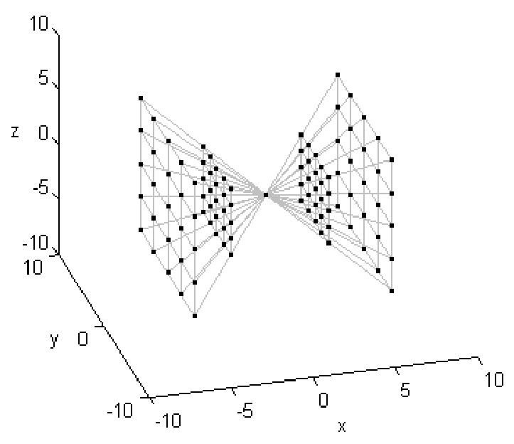
(a) The sector $\Omega_{ppx}$ for $n=4$

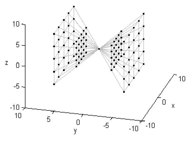
(b) The sector $\Omega_{ppy}$ for $n=4$

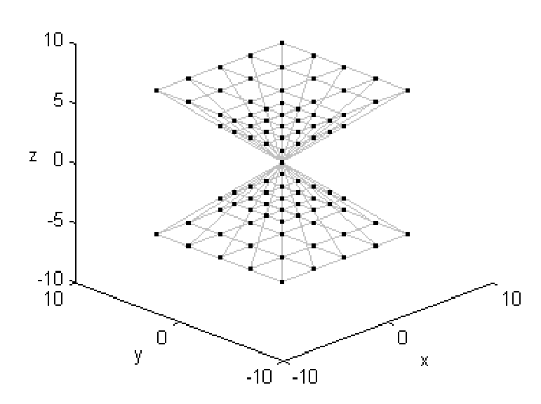
(c) The sector $\Omega_{ppz}$ for $n=4$

Figure 1: The three sectors $\Omega_{ppx},\Omega_{ppx}$ and $\Omega_{ppz}$ that form the 3D pseudo-polar grid.

Next, we define the discrete time Fourier transform of an $n\times n\times n$ volume $I$ by

$$\hat{I}(\omega_{x},\omega_{y},\omega_{z})=\sum_{u,v,w=-n/2}^{n/2-1}I(u,v,w)\,e^{2\pi\imath(u\omega_{x}+v\omega_{y}+w\omega_{z})/m},\quad\omega_{x},\omega_{y},\omega_{z}\in[-m/2,m/2],$$ (3)

where as before $m=qn+1$ for an even $n$ and a positive integer $q$. The three-dimensional pseudo-polar Fourier transform (PPFT) is defined as the samples of the discrete time Fourier transform of Eq. 3 on the pseudo-polar grid $\Omega_{pp}$. Specifically, if we denote the concatenation of three arrays $A_{1}$, $A_{2}$, and $A_{3}$ by $A=\left[A_{1},A_{2},A_{3}\right]$, then the pseudo-polar Fourier transform of a volume $I\in\mathbb{C}^{n\times n\times n}$ is an array $\hat{I}_{\Omega_{pp}}\in\mathbb{C}^{3\times(n+1)\times(n+1)\times(3n+1)}$ given by

$$\hat{I}_{\Omega_{pp}}=\left[\hat{I}_{\Omega_{ppx}},\hat{I}_{\Omega_{ppy}},\hat{I}_{\Omega_{ppz}}\right],$$ (4)

where

$$\hat{I}_{\Omega_{ppx}}=\hat{I}\left(k,-\frac{2l}{n}k,-\frac{2j}{n}k\right),\quad\hat{I}_{\Omega_{ppy}}=\hat{I}\left(-\frac{2l}{n}k,k,-\frac{2j}{n}k\right),\quad\hat{I}_{\Omega_{ppz}}=\hat{I}\left(-\frac{2l}{n}k,-\frac{2j}{n}k,k\right),$$ (5)

and $\Omega_{ppx},\Omega_{ppy}$ and $\Omega_{ppz}$ are defined in Eq. 2. The parameter $q$ in Eqs. 1 and  3 determines the frequency resolution of the transform, as well as its geometric properties. For example, as shown in [3], in order to derive a three-dimensional discrete Radon transform based on the pseudo-polar Fourier transform, $q$ must satisfies $q\geq 3$.

The pseudo-polar grid appeared in the literature several times under different names. It was originally introduced by [35] under the name “Concentric Squared Grid” in the context of computerized tomography. More recent works in the context of computerized tomography, which take advantage of the favorable numerical and computational properties of the grid include [33, 34], where equally sloped tomography is used for radiation dose reduction. Other image processing applications that use the pseudo-polar grid include synthetic aperture radar (SAR) imaging [28], Shearlets [27, 26], registration [32], and denoising [41], to name a few.

Recently, [39] proposed fast iterative inversion algorithms for the 2D and 3D pseudo-polar Fourier transforms, which are based on the well-known convolution structure of their Gram operators, combined with a preconditioned conjugate gradients [18] solver. The convolution structure of the transform allows to invert it using the highly optimized FFT algorithm instead of the forward and adjoint transforms derived in [2]. As the conjugate gradients iterations require preconditioning, [39] proposes a preconditioner that leads to a very small condition number, thus making the inversion process fast and accurate. However, this approach has drawbacks such as high memory requirements and dependency of the number of iterations and on the size of the data. The algorithm presented in this paper, which has a low memory requirements, achieves high accuracy and is faster than the iterative algorithm [39].

2.2 Solving Toeplitz systems

Let $A_{n}$ be an $n\times n$ Toeplitz matrix and let $y$ be an arbitrary vector of length $n$. We describe a fast algorithm for computing $A_{n}^{-1}y$. This algorithm is well-known and appears, for example, in [2], but we repeat it here for completeness of the description. The algorithm consists of a fast factorization of the inverse Toeplitz matrix followed by a fast algorithm that applies the inverse matrix to a vector [17, 24]. We denote by $T_{n}(c,r)$ an $n\times n$ Toeplitz matrix whose first column and row are $c$ and $r$, respectively. For symmetric matrices, $c=r$.

Circulant matrices are diagonalized by the Fourier matrix. Hence, a circulant matrix $C_{n}$ can be written as $C_{n}=W^{*}_{n}D_{n}W_{n},$ where $D_{n}$ is a diagonal matrix containing the eigenvalues $\lambda_{1},\ldots,\lambda_{n}$ of $C_{n}$, and $W_{n}$ is the Fourier matrix given by $W_{n}(j,k)=\frac{1}{\sqrt{n}}e^{2\pi\imath jk/n}$. Moreover, if $c=[c_{0},c_{1},\ldots,c_{n-1}]^{T}$ is the first column of $C_{n}$, then $W_{n}c=[\lambda_{1},\ldots,\lambda_{n}]^{T}$. Obviously, the matrices $W_{n}$ and $W_{n}^{*}$ can be applied in $O(n\log{n})$ operations using the FFT. Thus, the multiplication of $C_{n}$ with an arbitrary vector $x$ of length $n$ can be implemented in $O(n\log{n})$ operations by applying FFT to $x$, multiplying the result by $D_{n}$, and then applying the inverse FFT.

To compute $A_{n}x$ for an arbitrary Toeplitz matrix $A_{n}=T_{n}(c,r)$ and an arbitrary vector $x$, we first embed $A_{n}$ in a $2n\times 2n$ circulant matrix $C_{2n}$

$$C_{2n}=\left(\begin{array}[]{cc}A_{n}&B_{n}\\ \vskip 3.0pt plus 3.0pt minus 1.0pt\cr B_{n}&A_{n}\end{array}\right),$$

where $B_{n}$ is an $n\times n$ Toeplitz matrix given by

$$B_{n}=T_{n}([0,r_{n-1},\ldots,r_{2},r_{1}],[0,c_{n-1},\ldots,c_{2},c_{1}]).$$

Then, $A_{n}x$ is computed in $O(n\log{n})$ operations by zero padding $x$ to length $2n$, applying $C_{2n}$ to the padded vector, and discarding the last $n$ elements of the resulting vector.

Next, assume that $A_{n}$ is invertible. The Gohberg–Semencul formula [17, 16] provides an explicit representation of $A_{n}^{-1}$ as

$$A_{n}^{-1}=\frac{1}{x_{0}}\left(M_{1}M_{2}-M_{3}M_{4}\right),$$ (6)

where

$$M_{1} =T_{n}([x_{0},x_{1},\ldots,x_{n-1}],[x_{0},0,\ldots,0]),$$ (7)

$$M_{2} =T_{n}([y_{n-1},0,\ldots,0],[y_{n-1},y_{n-2},\ldots,y_{0}]),$$ (8)

$$M_{3} =T_{n}([0,y_{0},\ldots,y_{n-2}],[0,\ldots,0]),$$ (9)

$$M_{4} =T_{n}([0,\ldots,0],[0,x_{n-1},\ldots,x_{1}]),.$$ (10)

The vectors $x=[x_{0},\ldots,x_{n-1}]$ and $y=[y_{0},\ldots,y_{n-1}]$ are given as the solutions to

$$A_{n}x = e_{0}, e_{0} =[1,0,\ldots,0]^{T},$$ (11)

$$A_{n}y = e_{n-1}, e_{n-1} =[0,\ldots,0,1]^{T}.$$

The matrices $M_{1}$, $M_{2}$, $M_{3}$, and $M_{4}$ have Toeplitz structure and are represented implicitly using the vectors $x$ and $y$. Hence, the total storage required to store $M_{1}$, $M_{2}$, $M_{3}$, and $M_{4}$ is that of $2n$ numbers. If the matrix $A_{n}$ is fixed, then the vectors $x$ and $y$ can be precomputed. Once the triangular Toeplitz matrices $M_{1}$, $M_{2}$, $M_{3}$ and $M_{4}$ have been computed, the application of $A_{n}^{-1}$ is reduced to the application of four Toeplitz matrices. Thus, the application of $A_{n}^{-1}$ to a vector requires $O(n\log{n})$ operations. The pseudo-code of applying $A_{n}^{-1}$ to a vector is described in Algorithms 7, 8, and 9 in the appendix. Algorithm 7 lists the function ToeplitzDiag, which computes the diagonal form of the circulant embedding of a Toeplitz matrix. Algorithm 8 lists the function ToeplitzInvMul, which efficiently multiplies an inverse Toeplitz matrix, given in its diagonal form, by a vector. The latter function uses ToeplitzMul, listed in Algorithm 9, which efficiently multiplies a general Toeplitz matrix by a vector.

2.3 Resampling trigonometric polynomials

The main (and in fact the only) tool behind our algorithm is resampling of univariate trigonometric polynomials. Assume we are given a set of points $\{y_{j}\}_{j=1}^{N}$, $y_{j}\in[-\pi,\pi]$, and their values $\{f(y_{j})\}_{j=1}^{N}$, where $f$ is some unknown univariate trigonometric polynomial of degree $n\leq N$. We want to estimate the values of $f$ at a new set of points $\{x_{j}\}_{j=1}^{M}$, $x_{j}\in[-\pi,\pi]$. This can be formulated by first solving

$$\min_{\alpha}\sum_{j=1}^{N}\left|f(y_{j})-\sum_{k=-n/2}^{n/2-1}\alpha_{k}e^{\imath ky_{j}}\right|^{2},\quad\alpha=\left(a_{-n/2},\ldots,\alpha_{n/2-1}\right)\in\mathbb{C}^{n},$$ (12)

for the coefficients vector $\alpha$, followed by evaluating

$$f(x_{i})=\sum_{k=-n/2}^{n/2-1}\alpha_{k}e^{\imath kx_{i}}.$$ (13)

In matrix notation, Eq. 12 is written

$$\min_{\alpha}\|f-A\alpha\|_{2},$$ (14)

where the entries of the matrix $A$ are given by $a_{jk}=e^{\imath ky_{j}}$ and the coordinates of the vector $f$ are $f_{j}=f(y_{j})$ (we denote by $f$ both the vector and the function, as the appropriate meaning is clear from the context). Direct solution for the coefficients vector $\alpha$ requires $\mathcal{O}(n^{3})$ operations (assuming $N$ and $M$ are of size $O(n)$). Obviously, solving for $\alpha$ also depends on the condition number of $A$, which affects the accuracy of $f(x_{i})$.

We next present a fast algorithm for computing $f(x_{i})$ (faster than directly solving first for $\alpha$), which exploits the Toeplitz structure of $A^{*}A$ and uses the non-equally spaced FFT (NUFFT) [8, 10, 15, 14, 36, 20]. The resulting algorithm has complexity of $\mathcal{O}(n\log n+n\log 1/\epsilon)$ operations, where $\epsilon$ is the accuracy of the computations, in addition to a preprocessing step that takes $\mathcal{O}(n^{2})$ operations.

Following [19], we define the NUFFT type-I by

$$f_{k}=\frac{1}{n_{j}}\sum_{j=1}^{n_{j}}c_{j}e^{\pm\imath kx_{j}},\quad k=-n/2,\ldots,n/2-1.$$ (15)

and the NUFFT type-II by

$$c_{j}=\sum_{k=-n/2}^{n/2-1}f_{k}e^{\pm\imath kx_{j}},\quad j=1,...,n_{j}.$$ (16)

Both types can be approximated to a relative accuracy $\epsilon$ in $\mathcal{O}(n\text{log}n+n\log 1/\epsilon)$ operations by any of the aforementioned NUFFT algorithms. From the definitions of NUFFT of types I and II, we see that $A^{*}f$, where $A$ is the matrix from Eq. 14 and $f$ is an arbitrary vector, is equal to the application of NUFFT type-I to $f$. Similarly, the application of $A$ to an arbitrary vector $c$ is equal to the application of NUFFT type-II to $c$. Hence, the application of $A$ or $A^{*}$ to a vector can be implemented in $\mathcal{O}(n\log n+n\log 1/\epsilon)$ operations.

To solve the least-squares problem of Eq. 14 we form the normal equations

$$A^{*}A\alpha=A^{*}f.$$ (17)

The right-hand side in Eq. 17 can be computed efficiently using NUFFT type-I. The matrix $A^{*}A$ is a symmetric Toeplitz matrix of size $n\times n$. The first column of $A^{*}A$, which due to the symmetric Toeplitz structure encodes all its entries, is computed efficiently by applying NUFFT type-I to the vector $w$ whose entries are $w_{j}=e^{-\imath ny_{j}/2}$. Computing $(A^{*}A)^{-1}$ takes $\mathcal{O}(n^{2})$ operations using the Durbin-Levinson algorithm [31] and applying it to a vector takes $\mathcal{O}(n\log n)$ operations using the Gohberg-Semencul formula [23], as was described in Section 2.2. This procedure is described in details in [2]. Since $(A^{*}A)^{-1}$ depends only on $n$, it can be precomputed. Therefore, solving for $\alpha$ in Eq. 17 takes $\mathcal{O}(n\log n+n\log 1/\epsilon)$ operations and computing $f(x_{i})$ in Eq. 13 takes additional $\mathcal{O}(n\log n+n\log 1/\epsilon)$ operations using NUFFT type-II. The entire resampling algorithm is described in Algorithm 5.

3 Direct inversion of the 3D PPFT

Given the PPFT $\hat{I}_{\Omega_{pp}}$ defined in Eq. 4 of an unknown $n\times n\times n$ volume $I$, the proposed direct inversion algorithm recovers $I$ in two steps. The first step resamples the PPFT into an intermediate Cartesian grid. Specifically, we resample the trigonometric polynomial $\hat{I}$ of Eq. 3 from the grid $\Omega_{pp}$ in Eq. 1 to the frequency grid

$$\Omega_{c}=\{(qu,qv,qw):u,v,w=-n/2,...,n/2\}.$$ (18)

The second step of our algorithm recovers $I$ from the samples of $\hat{I}$ on $\Omega_{c}$. Note that this second step cannot be directly implemented by inverse FFT. The two steps of the algorithm are described in Sections 3.1 and 3.2, respectively, its pseudo-code is given in Algorithm 1, and its complexity is analyzed in Section 3.3.

3.1 Resampling the pseudo-polar grid to the grid $\Omega_{c}$

We start by describing the procedure for resampling $\hat{I}$ from $\Omega_{pp}$ to $\Omega_{c}$. It is based on an “onion peeling” approach, which resamples at iteration $k$, $k=n/2,\ldots,0$, points in $\Omega_{pp}$ with “pseudo-radius” $k$ to points in $\Omega_{c}$ that lie on a plane. When the iteration that corresponds to $k=0$ is completed, the values of $\hat{I}$ have been computed on all points of the grid $\Omega_{c}$. We define the sets $\Omega_{c}^{(k)}\subseteq\Omega_{c}$, $k=n/2,\ldots,0$, consisting of the frequencies on which $\hat{I}$ has been resampled until (and including) iteration $k$. Note that for convenience, we index the iterations from $k=n/2$ to $k=0$. Thus, we have that $\Omega_{c}^{(k)}\subseteq\Omega_{c}^{(k-1)}$ and $\Omega_{c}^{(0)}=\Omega_{c}$. Formally, we define $\Theta^{(k)}$ to be the frequencies on which we resample $\hat{I}$ at iteration $k$ so that

$$\Omega_{c}^{(k)}=\Omega_{c}^{(k+1)}\cup\Theta^{(k)},$$

where $\Theta^{(k)}$ is give by

$$\Theta^{(k)}=\Theta^{(k)}_{+x}\cup\Theta^{(k)}_{-x}\cup\Theta^{(k)}_{+y}\cup\Theta^{(k)}_{-y}\cup\Theta^{(k)}_{+z}\cup\Theta^{(k)}_{-z},$$ (19)

and for $j,l=-k,\ldots,k$

$$\Theta^{(k)}_{+x} = \{(qk,qj,ql)\}, \Theta^{(k)}_{-x} = \{(-qk,qj,ql)\},$$ (20)

$$\Theta^{(k)}_{+y} = \{(qj,qk,ql)\}, \Theta^{(k)}_{-y} = \{(qj,-qk,ql)\},$$

$$\Theta^{(k)}_{+z} = \{(qj,ql,qk)\}, \Theta^{(k)}_{-z} = \{(qj,ql,-qk)\}.$$

For $k=n/2$ we set $\Omega_{c}^{(n/2)}=\Theta^{(n/2)}$. Moreover, the frequencies of $\Theta^{(n/2)}$ are the frequencies $\Omega_{ppx}(\pm n/2,j,l)$, $\Omega_{ppy}(\pm n/2,j,l)$, and $\Omega_{ppz}(\pm n/2,j,l)$, $l,j=-n/2,\ldots,n/2$, defined in Eq. 2. Thus, the values of $\hat{I}$ on $\Omega_{c}^{(n/2)}$ are given as a subset of the values of $\hat{I}$ on $\Omega_{pp}$. Therefore, no resampling is needed at this iteration.

For subsequent iterations, we use an example to accompany and clarify the formal description. We use as an example a grid corresponding to $n=8$ that demonstrates how the values of $\hat{I}$ on $\Theta^{(n/2-1)}$ (which is $\Theta^{(3)}$ in our particular example) are recovered. Since the same procedure recovers the values of $\hat{I}$ on $\Theta^{(k)}_{\pm x}$, $\Theta^{(k)}_{\pm y}$, and $\Theta^{(k)}_{\pm z}$, we only explain the process for the grid $\Theta^{(k)}_{+x}$. The pseudo-code for recovering the values of $\hat{I}$ on $\Theta^{(k)}$ is given in Algorithm 2, whose details are also explained below.

In Fig. 2a, green solid squares correspond to points from $\Omega_{c}^{(k+1)}$ on which $\hat{I}$ has already been evaluated (in previous iterations), red circles correspond to points from $\Omega_{ppx}$ with a fixed $k=n/2-1$, and blue dots correspond to points of $\Theta^{(k)}_{+x}$ on which we want to evaluate $\hat{I}$. The frequencies in $\Theta^{(k)}_{+x}$ are points in $\mathbb{R}^{3}$, however, as can be seen from Eq. 20, they all lie on the same plane, and therefore, we depict them as a two-dimensional image whose axes are $i$ and $j$ from Eq. 20.

(a) Beginning of iteration $k=n/2-1$

(b) Resampling of $\hat{I}$ to the set $\Theta^{(k)}_{x}$

Figure 2: The grid before and after the applications of lines $11-14$ in Algorithm 2. Green solid squares correspond to points from $\Omega_{c}^{(k+1)}$, red circles correspond to points from $\Omega_{ppx}$ with a fixed $k=n/2-1$, blue dots correspond to points of $\Theta^{(k)}_{+x}$, and patterned yellow points correspond to point of $\Omega_{c}^{(k+1)}$ resampled to their intermediate position.

The first step, depicted in Fig. 2b, consists of resampling the points of $\Omega_{c}^{(k+1)}$ (solid green squares) to the same spacing as the pseudo-polar points. In the case of $k=n/2-1$, this means that the first and the last rows are resampled, and the result of this resampling is denoted by patterned yellow squares. This step is implemented by lines $11-14$ in Algorithm 2. Next, as depicted in Fig. 3a, for all columns, we use the latter resampled points (patterned yellow squares) together with the points of the pseudo-polar grid at the same column to resample $\hat{I}$ to intermediate sampling points. Figures 3a and 3b depict the resampling of one such column. Note that the resampled values of $\hat{I}$ after this step, which are depicted as filled teal circles in Fig. 3b, are not yet the values of $\hat{I}$ on the points of $\Theta^{(k)}_{x}$. Up to here, we only applied resampling to the columns (but not yet to rows). We repeat this for all the columns (see Fig. 4a for resampling of another column), which results in the grid of Fig. 4b. This is implemented by lines $18-20$ of Algorithm 2, which using the conventions of Fig. 4, resamples the red circles along the columns to the filled teal circle, which are now on the same rows as the points indicated by the blue dots (our target sampling points). Next, we apply one-dimensional resampling to each row, by using the resampled points from the previous steps together with the points of $\Omega_{c}^{(k+1)}$ (Fig. 5a) to recover the samples of $\Theta_{x}^{(k)}$ (Fig. 5b). This is implemented by lines $22-24$ of Algorithm 2. All one-dimensional resampling operations in Algorithm 2 are implemented using the function ToeplitzResample in Algorithm 5.

(a) Before resampling

(b) After resampling

Figure 3: The grid before and after the applications one iteration of lines $18-20$ in Algorithm 2.

(a) Before resampling

(b) After resampling

Figure 4: The grid before and after further iterations of lines $18-20$ in Algorithm 2.

(a) Before resampling

(b) After resampling

Figure 5: The grid before and after the application of lines $22-24$ in Algorithm 2 (row resampling).

Algorithm 1 Direct inversion of the 3D pseudo-polar Fourier transform.

1:Input: Samples of the 3D pseudo-polar Fourier transform $\hat{I}_{\Omega_{ppx}},\hat{I}_{\Omega_{ppy}},\hat{I}_{\Omega_{ppz}}$, given by Eq. 5, each of size $(qn+1)\times(n+1)\times(n+1)$.

2:Output: Volume $I$ of size $n\times n\times n$.

3: $\hat{I}_{D}\leftarrow\operatorname{zeros}(n+1,n+1,n+1)$

4:for $j=1,\ldots,n/2$ do

5:     $\hat{I}_{D}(j,:,:)\leftarrow\operatorname{\texttt{recover2d}}(\hat{I}_{\Omega_{ppx}}(q(j-1)+1,:,:),\hat{I}_{D}(j,:,:),j-1)$    $\triangleright$ Algorithm 2

6:     $\hat{I}_{D}(n+2-j,:,:)\leftarrow\operatorname{\texttt{recover2d}}(\hat{I}_{\Omega_{ppx}}(qn-q(j-1)+1,n+1:-1:1,n+1:-1:1),\hat{I}_{D}(n+2-j,:,:),j-1)$

7:     $\hat{I}_{D}(:,j,:)\leftarrow\operatorname{\texttt{recover2d}}(\hat{I}_{\Omega_{ppy}}(q(j-1)+1,:,:),\hat{I}_{D}(:,j,:),j-1)$   

8:     $\hat{I}_{D}(:,n+2-j,:)\leftarrow\operatorname{\texttt{recover2d}}(\hat{I}_{\Omega_{ppy}}(qn-q(j-1)+1,n+1:-1:1,n+1:-1:1),\hat{I}_{D}(:,n+2-j,:),j-1)$

9:     $\hat{I}_{D}(:,:,j)\leftarrow\operatorname{\texttt{recover2d}}(\hat{I}_{\Omega_{ppz}}(q(j-1)+1,:,:),\hat{I}_{D}(:,:,j),j-1)$   

10:     $\hat{I}_{D}(:,:,n+2-j)\leftarrow\operatorname{\texttt{recover2d}}(\hat{I}_{\Omega_{ppz}}(qn-q(j-1)+1,n+1:-1:1,n+1:-1:1),\hat{I}_{D}(:,:,n+2-j),j-1)$

11:end for

12:$\hat{I}_{D}(n/2+1,n/2+1,n/2+1)\leftarrow\hat{I}_{\Omega_{ppx}}(3n/2+1,n/2+1,n/2+1)$ (center point)

13:${I}\leftarrow$InvDecimatedFreq($\hat{I}_{D}$) $\triangleright$ (recover $I$ from $\hat{I}_{D}$ by Algorithm 4)

Algorithm 2 recover2d. This function recovers a 2D slice of the 3D pseudo-polar grid and recovers it to Cartesian grid (resample $\hat{I}$ from the set $\Omega_{c}^{(k+1)}$ to the set $\Theta^{(k)}$.)

1:Input: $\hat{U}_{\Omega_{ppx}}$ - Slice of the 3D pseudo-polar Fourier transform of size $(n+1)\times(n+1)$. $\hat{U}_{D}$ - Already resampled slice of $\hat{I}_{D}$ from Algorithm 1 of size $(n+1)\times(n+1)$. $j$ - An integer indicating the stage within the peeling procedure.

2:Output: $result$ of size $(n+1)\times(n+1)$ (resampled part, $\hat{I}_{D}$ from Algorithm 1)

3:$\alpha\leftarrow(n/2-j)/(n/2)$

4:$m\leftarrow qn+1$

5:if $j==0$ then

6:     $result\leftarrow\hat{U}_{\Omega_{pp}}$ return

7:end if

8:$y_{1}\leftarrow[-n/2:n/2]\times(-2)\times q\times\pi/m$

9:$x_{1}\leftarrow[-n/2:n/2]\times(-2)\times q\times\alpha\times\pi/m$

10:$C\leftarrow\operatorname{zeros}(n+1,n+1)$

11:for $k=1,\ldots,j$ do

12:     $C(k,:)\leftarrow\texttt{ToeplitzResample}\left(\hat{U}_{\Omega_{pp}}(k,1:n+1),y_{1},x_{1}\right)$ $\triangleright$ Algorithm 5

13:     $C(n+2-k,:)\leftarrow\texttt{ToeplitzResample}\left(\hat{U}_{\Omega_{pp}}(n+2-k,1:n+1)y_{1},x_{1}\right)$

14:end for

15:$x\leftarrow[-(n/2-j):(n/2-j)]\times(-2)\times q\times\pi/m$

16:$y\leftarrow\left[[-n/2:-n/2+j-1],[-n/2:n/2]\times\alpha,[n/2-j+1:n/2]\right]\times(-2)\times q\times\pi/m$

17:$R_{1}\leftarrow\operatorname{zeros}(n+1-2j,n+1)$

18:for $k=1,\ldots,n+1$ do

19:     $R_{1}\leftarrow\texttt{ToeplitzResample}\left(\left[C(1:j,k),\hat{U}_{\Omega_{pp}}(:,k),C(n-j+2:n+1,k)\right],y,x\right)$

20:end for

21:$R_{2}\leftarrow\operatorname{zeros}(n+1-2j,n+1-2j)$

22:for $k=1,\ldots,n+1-2j$ do

23:     $R_{2}\leftarrow\texttt{ToeplitzResample}\left(\left[\hat{U}_{D}(k+j,1:j),R_{1}(k,:),\hat{U}_{D}(k+j,n-j+2:n+1)\right],y,x\right)$

24:end for

25:$result\leftarrow\hat{U}_{D}$

26:$result(1+j:n+1-j,1+j:n+1-j)\leftarrow R_{2}$

3.2 Recovering $I$ from $\hat{I}$ on $\Omega_{c}$

The second step in Algorithm 1 (line 11) recovers the volume $I$ from the samples in $\hat{I}$ on $\Omega_{c}$ (see Eq. 18). Define the operator $F_{D}:\mathbb{C}^{n}\to\mathbb{C}^{n+1}$, by

$$(F_{D}u)_{k}=\sum_{j=-n/2}^{n/2-1}u(j)e^{-2\pi\imath jqk/m},\quad k=-n/2,\ldots,n/2,\quad m=qn+1.$$ (21)

For a volume $I$ of size $n\times n\times n$, we denote by $F_{D}^{(x)}$, $F_{D}^{(y)}$ and $F_{D}^{(z)}$ the application of $F_{D}$ to the $x$, $y$ and $z$ directions of $I$, respectively. Furthermore, we define

$$\tilde{I}=F_{D}^{(z)}F_{D}^{(y)}F_{D}^{(x)}I.$$ (22)

From the definitions of $F_{D}$, $\hat{I}$ and $\Omega_{c}$ in Eqs.  21, 3 and 18, respectively, we conclude that $\tilde{I}$ is equal to the samples of $\hat{I}$ on the grid $\Omega_{c}$. Thus, if we apply the inverse of $F_{D}$ to the $x$, $y$, and $z$ dimensions of $\tilde{I}$ (in a separable way), we recover $I$ from the samples of $\hat{I}$ on $\Omega_{c}$. The inversion of the operator $F_{D}$ is described in [2]. Specifically, in our case, for $m=qn+1$, the adjoint of $F_{D}$ is given by

$$(F^{*}_{D}w)_{j}=\sum_{k=-n/2}^{n/2}w_{k}e^{2\pi\imath jqk/m},\quad j=-n/2,\ldots,n/2-1.$$

The matrix $F^{*}_{D}F_{D}$ is a Toeplitz matrix, whose entries are given by

$$(F^{*}_{D}F_{D})_{k,l}=\sum_{j=-n/2}^{n/2}e^{2\pi\imath qj(k-l)/m},\quad k,l=-n/2,\ldots,n/2-1,$$

and its inverse is applied as described in Eq. 6. The image $I$ is recovered by the application of $(F_{D}^{*}F_{D})^{-1}F_{D}^{*}$ to each dimension of $\widetilde{I}$. Accurately recovering $I$ from $\tilde{I}$ requires the condition number of $F^{*}_{D}F_{D}$ to be small. The maximal condition number of $F_{D}$, which was obtained while applying Algorithm 2 to various sizes $n$, is illustrated in Fig. 6. The reason the term “maximal” is used, is since during the running of the algorithm, several operators $F_{D}$ are used for a given $n$. As can be seen, the condition number is less than 25 even for very large volumes. The operator $F_{D}^{*}$ is applied efficiently to a vector $w$ by adding $q-1$ zeros between every two samples of $w$, applying the inverse FFT to the resulting vector, and keeping the $n$ central elements of the FFT-transformed vector (see Algorithm 3 for a detailed description). The pseudo-code of the algorithm for recovering the volume from its samples in $\Omega_{c}$ is described in Algorithm 4.

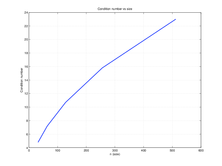
Figure 6: The maximal condition number of $F_{D}$ (see Eq. 21) obtained while applying Algorithm 4 to various sizes $n$.

Algorithm 3 AdjFDecimated: Applying $F_{D}^{*}$ of Eq. 21 to a vector

1:Input: $y$ - Input vector of odd length.

2:$q$ - integer (decimation factor).

3:Output: $x=F_{D}^{*}y$

4:$n\leftarrow$length$(y)-1$

5:$m\leftarrow qn+1$

6:$z\leftarrow\operatorname{zeros}(m,1)$

7:$z(1:q:m)\leftarrow y$

8:$l\leftarrow$length$(z)$

9:$p_{f}\leftarrow$ floor$(l/2)$

10:$p_{c}\leftarrow$ ceil$(l/2)$

11:$x\leftarrow z([p_{f}+1:l,~{}1:p_{f}])$

12:$x_{IFFT}\leftarrow$IFFT$(x)$

13:$x\leftarrow m\cdot x_{IFFT}([p_{c}+1:l,~{}1:p_{c}])$

14:$x\leftarrow x(n+1:2n)$

Algorithm 4 InvDecimatedFreq. This procedure inverts the decimated frequencies and restores $I$ from $\tilde{I}$ of Eq. Eq. 22

1:Input: $\tilde{I}$ - Matrix of size $(n+1)\times(n+1)\times(n+1)$.

2:Output: $I$ - Volume of size $n\times n\times n$ such that Eq. 22 holds.

3:$c\leftarrow$ zeros$(n,1)$

4:$m\leftarrow qn+1$

5:for  $k=-n/2,\ldots,n/2-1$ do

6:     for  $l=-n/2,\ldots,n/2$ do

7:         $c(k+n/2+1)\leftarrow c(k+n/2+1)+e^{q\pi\imath l(-n/2-k)/m}$

8:     end for

9:end for

10:$(M_{1},M_{2},M_{3},M_{4})\leftarrow$ ToeplitzInv($c$) $\triangleright$ Algorithm 6

11:$D_{i}\leftarrow$ ToeplitzDiag($M_{i}$),  $i=1,\ldots,4$ $\triangleright$ Algorithm 7

12:$I_{1}\leftarrow\operatorname{zeros}(n+1,n+1,n)$

13:$I_{2}\leftarrow\operatorname{zeros}(n+1,n,n)$

14:$I\leftarrow\operatorname{zeros}(n,n,n)$

15:for  $k=1,\ldots,n+1$ do

16:     for  $l=1,\ldots,n+1$ do

17:         $v\leftarrow\widetilde{I}(k,l,:)$

18:         $v\leftarrow$AdjFDecimated$(v)$ $\triangleright$ Algorithm 3

19:         $u\leftarrow$ToeplitzInvMul$(D_{1},D_{2},D_{3},D_{4},v)$ $\triangleright$ Algorithm 8

20:         $I_{1}(k,l,:)\leftarrow u$

21:     end for

22:end for

23:for  $k=1,\ldots,n+1$ do

24:     for  $l=1,\ldots,n$ do

25:         $v\leftarrow I_{1}(k,:,l)$

26:         $v\leftarrow$AdjFDecimated$(v)$

27:         $u\leftarrow$ToeplitzInvMul$(D_{1},D_{2},D_{3},D_{4},v)$

28:         $I_{2}(k,l,:)\leftarrow u$

29:     end for

30:end for

31:for  $k=1,\ldots,n$ do

32:     for  $l=1,\ldots,n$ do

33:         $v\leftarrow I_{2}(:,k,l)$

34:         $v\leftarrow$AdjFDecimated$(v)$

35:         $u\leftarrow$ToeplitzInvMul$(D_{1},D_{2},D_{3},D_{4},v)$

36:         $I(:,k,l)\leftarrow u$

37:     end for

38:end for

3.3 Complexity Analysis

The inversion Algorithm 1 consists of two steps: Resampling (lines 1-12) and recovering $I$ from $\hat{I}$ on $\Omega_{c}$ (line 13). The first step, resampling, which utilizes Toeplitz matrices (Algorithm 5), takes $\mathcal{O}(n\text{log}n)$ operations when preprocessing took place. This function (Toepliz-based resampling) is called $\mathcal{O}(n)$ times in the $\operatorname{\texttt{recover2d}}$ function (Algorithm 2), which in turn is called also $\mathcal{O}(n)$ times by Algorithm 1. A total of $\mathcal{O}(n^{3}\text{log}n)$ operations are needed for the resampling step.

The second step, recovering $I$ from $\hat{I}$ on $\Omega_{c}$, takes $\mathcal{O}(n^{3}\text{log}n)$ operations. This yields a total computational complexity of $\mathcal{O}(n^{3}\text{log}n)$ operations. If the preprocessing is done in run time, the total complexity becomes $\mathcal{O}(n^{4})$ operations, due to the Durbin-Levinson algorithm used for inverting Toeplitz matrices. The computational complexity can be reduced from $\mathcal{O}(n^{4})$ operations to $\mathcal{O}(n^{3}\text{log}^{2}n)$ by solving Eq. 11 as described in [23].

The total storage requirement for $n$ applications of Algorithm 2 is $4n^{2}$. This storage is used to store the diagonal Toeplitz matrices $D_{1},\ldots,D_{4}$.

4 Numerical results

We implemented Algorithm 1 in MATLAB and applied it to several volumes of sizes $n\times n\times n$ where $n=32,64,...,512$. All the experiments were executed on a Linux machine with two Intel Xeon processors (CPU X5560) running at 2.8GHz, with 8 cores in total and $96$GB of RAM. All the 3D experiments were performed with $q=3$ (see Eq. 2).

Algorithm 2 is based on a series of one-dimensional resampling operations. We compare two methods for implementing this one-dimensional resampling – least-squares-based (LS) approach and Toeplitz-NUFFT-based approach, both described in Section 2.3. The LS-based approach, described in Eq. 12, consists of finding the coefficients vector $\alpha$ of a trigonometric polynomial, followed by direct evaluation of the polynomial at the resampling points. Using this resampling approach in Algorithm 2 results in computational complexity of $\mathcal{O}(n^{3})$ operations (excluding a preprocessing step). Nevertheless, its implementation in MATLAB is highly optimized. The Toeplitz-NUFFT-based approach, described in Section 2.3 and Algorithm 5, results in computational complexity of Algorithm 2 of $\mathcal{O}(n^{2}\text{log}n+n^{2}\log 1/\epsilon)$ operations. The two resampling methods are compared by using them as the underlying one-dimensional resampling in Algorithm 2. Both algorithms use a preprocessing step which is excluded from the reported running time. The error incurred by the two algorithms is measured by

$$E(I,I_{r})=\sqrt{\frac{\sum_{k,l,m}\left\lvert{I[k,l,m]-I_{r}[k,l,m]}\right\rvert^{2}}{\sum_{k,l,m}\left\lvert{I[k,l,m]}\right\rvert^{2}}},$$

where $I[k,m,n]$ is the original volume and $I_{r}[k,m,n]$ is the reconstructed volume. Running times for both methods for volumes of sizes $n\times n\times n$, where $n=32,64,...,512$, are shown in Fig. 7. The volumes in this experiment consist of PPFT transformed random independent samples from a normal distribution with zero mean and unit variance. Figure 8 compares between the reconstruction errors of Algorithm 5 and those of LS-based resampling. The results show that both methods are comparable in terms of accuracy.

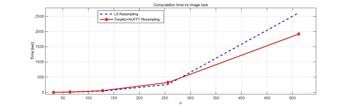
Figure 7: Runtime comparison between LS-based resampling and Toeplitz-NUFFT-based resampling (Algorithm 5) for volumes of sizes $n\times n\times n$, consisting of PPFT applied to a normally distributed i.i.d. random samples with zero mean and unit variance.

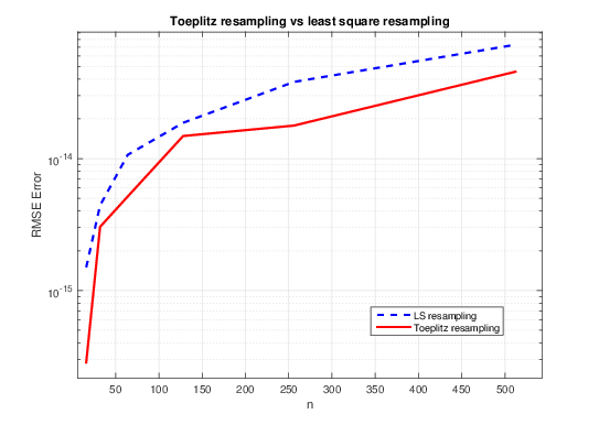
Figure 8: Error comparison between LS-based resampling and Toeplitz-NUFFT-based resampling (Algorithm 5) for volumes of sizes $n\times n\times n$, consisting of PPFT applied to a normally distributed random samples with zero mean and unit variance.

Since it is currently impossible to process 3D volumes of sizes larger than $n=512$, we compare between the LS-based resampling and the Toeplitz-based resampling by applying both one-dimensional resampling methods to a one-dimensional Chirp signal defined by $\cos(10k_{j}^{2})$, $k_{j}=-\pi+\frac{2\pi}{n}j$, $j=0,\ldots,n$, $n=512,\ 1024,\ 2048,\ 4096$. The signal’s samples given at $k_{j}$ were resampled to $0.3k_{j}$ using LS-based resampling and Toeplitz-based resampling. The one-dimensional Chirp signal is displayed in Fig. 9. The running time of the two methods, which does not include pre-processing timing, appears in Fig. 10. The approximation errors of both methods are practically identical as shown in Fig. 11.

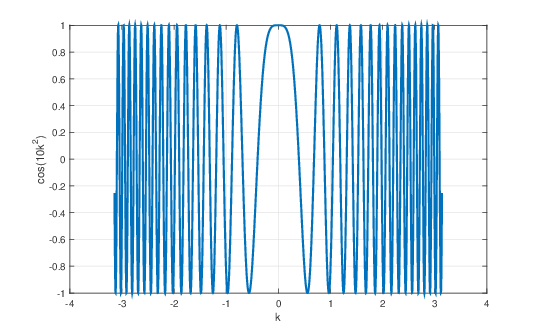
Figure 9: One-dimensional Chirp signal, used for testing the LS-based resampling and the Toeplitz-NUFFT-based resampling.

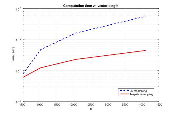
Figure 10: Runtime comparison between the LS-based resampling and the Toeplitz-NUFFT-based resampling (Algorithm 5) for a one-dimensional Chirp signal of length $n$.

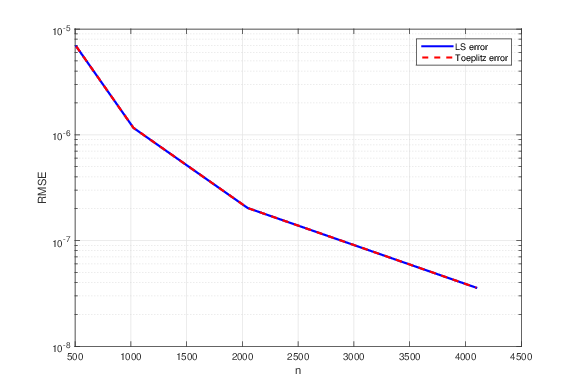
Figure 11: Error comparison between the LS-based resampling and Toeplitz-NUFFT-based resampling (Algorithm 5) for a one-dimensional chirp signal of length $n$.

Next, we compare between the direct inverse PPFT in Algorithm 1, the iterative algorithm described in [39], and a single iteration of an implementation that computes the Gram operator of the PPFT using the NUFFT as suggested by [13]. For the latter method, several iterations are required, whose number depends on the condition number of the operator. However, to keep all timings within the same scale, we compare the other two algorithms to only a single iteration of the latter one. The results are illustrated in Fig. 12, which shows that Algorithm 1 is faster than the iterative algorithm [39] as well as than a single iteration of the 3D NUFFT-based algorithm proposed by [13]. Results for $n=512$ do not appear in Fig. 12 (unlike Fig. 7) as it was impossible to process volumes of that size using [39, 13].

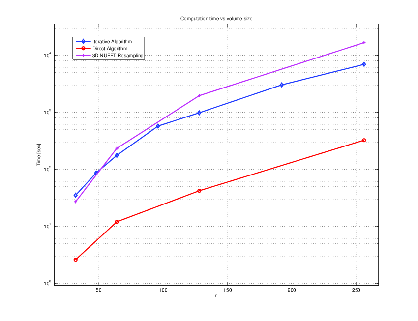
Figure 12: Comparison between the running time of Algorithm 1, the iterative algorithm [39], and the NUFFT-based algorithm [13].

Given the long running time of the 3D NUFFT-based algorithm, we executed above only a single iteration of this algorithm. However, to compare accuracy of our proposed method with that of the 3D NUFFT-based algorithm, we execute next the 3D NUFFT-based algorithm until the error becomes smaller than $10^{-12}$ or the number of iterations exceeds 100. Due to time constraints, we used only $n=16,\ 32,\ 64$. The input for each case was of size $n\times n\times n$ of random normally distributed i.i.d. samples with zero mean and unit variance. We implemented the 3D NUFFT-based algorithm with the same preconditioner as in [39]. For $n=16$ the algorithm took 112 seconds and the resulting error was $7.25\times 10^{-13}$, obtained after 40 iterations; for $n=32$, it took $2,710$ seconds with error of $7.5\times 10^{-13}$ after 100 iterations; for $n=64$ it took $22,477$ seconds (more than 6 hours) with error of $1.61\times 10^{-12}$ after 100 iterations. The iterative algorithm described in [39] gives similar errors to the direct inversion algorithm (Algorithm 1) whose error appears in Fig. 8.

Finally, we tested the algorithm on real volumes of different sizes: a dolphin of size $64\times 64\times 64$ (Fig. 13a), a bird of size $128\times 128\times 128$ (Fig. 13b), and a 3D cup of size $256\times 256\times 256$ (Fig. 13c). The volumes were taken from the McGill 3D shape dataset [40] and PPFT was applied to each one them to be used as an input for the inversion algorithm. The results appear in Table 1.

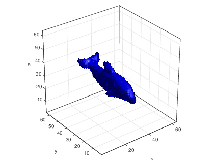
(a) Dolphin, $n=64$

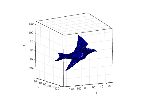
(b) Bird, $n=128$

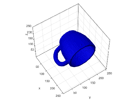
(c) Cup, $n=256$

Figure 13: Test volumes.

Name	Volume	Time [sec]	RMSE
Dolphin	$64\times 64\times 64$	7.43	$1.69\times 10^{-15}$
Bird	$128\times 128\times 128$	40.15	$3.6\times 10^{-15}$
Cup	$256\times 256\times 256$	270	$1.25\times 10^{-14}$

Table 1: Results for volumes of Fig. 13.

5 Conclusions

In this paper, a new algorithm for inverting the 3D pseudo-polar Fourier transform (PPFT) is described. The algorithm processes at each iteration a two-dimensional slice of the input, where each such processing uses only one-dimensional operations. The main component of the algorithm is fast resampling of univariate trigonometric polynomials. The resampling is implemented using a 1D non-uniform Fourier transform together with fast algorithms for Toeplitz matrices. The algorithm is not iterative, and requires a fixed amount of time that depends only on the size of the input. Moreover, the algorithm has low memory requirements, allowing to process large 3D datasets in a reasonable time. The performance of the algorithm is demonstrated on volumes as large as $512\times 512\times 512$ in double precision.

Appendix A Toeplitz solvers algorithms

Algorithm 5 ToeplitzResample: Fast resampling of a univariate trigonometric polynomial.

1:Input: $y$ - vector of length $n$.

2:$f$ - values of the trigonometric polynomial $\hat{I}$ on the set $y$.

3:$x$ - vector of length $n$.

4:Output: $g$ - values of $\hat{I}$ on the set $x$.

5:$k\leftarrow[-n/2:n/2-1]$ $\triangleright$ $k$ is a row vector

6:$c\leftarrow\text{length}(y)\times\text{NUFFT}_{1}(y,e^{\imath yk(1)},-1,n)$ $\triangleright$ $k(1)$ is the first element of $k$

7:$(M_{1},M_{2},M_{3},M_{4})\leftarrow$ ToeplitzInv$(c,c)$ $\triangleright$ Can be computed in the preprocessing step

8:for $i=1,\ldots,4$ do

9:     $D_{i}\leftarrow$ToeplitzDiag($M_{i}(:,1),M_{i}(1,:)$) $\triangleright$ Can be computed in the preprocessing step

10:end for

11:$v\leftarrow$ length $(y)\times$ NUFFT${}_{1}(y,f,-1,n)$

12:$\alpha\leftarrow$ToeplitzInvMul$(D_{1},D_{2},D_{3},D_{4},v)$

13:$g\leftarrow$ NUFFT₂ $(x,1,n,\alpha)$

NUFFT_k ($k=1,2$) refers to the type of the NUFFT - see Eqs.  15 and 16. The parameters $-1$ and $1$ in lines $6,11,13$ in Algorithm 5 refer to the sign of $\imath$ in the complex exponent. The function ToeplitzInv is described in Algorithm 6 and computes the Gohberg-Semencul factorization of a symmetric Toeplitz matrix.

Algorithm 6 ToeplitzInv: Factorize a symmetric Toeplitz matrix using the Gohbcerg-Semencul formula.

1:Input: $c$ - First column (row) of a symmetric Toeplitz matrix.

2:Output: $M_{1},M_{2},M_{3},M_{4}$ - Gohberg-Semencul factorization.

3:$n\leftarrow$length$(c)$

4:$e_{0}\leftarrow\operatorname{zeros}(n,1)$

5:$e_{n}\leftarrow\operatorname{zeros}(n,1)$

6:$e_{0}(1)\leftarrow 1$

7:$e_{n}(n)\leftarrow 1$

8:Solve $T_{n}(c,c)x=e_{0}$

9:Solve $T_{n}(c,c)y=e_{n}$

10:Compute $M_{1}$ using Eq. 7

11:Compute $M_{2}$ using Eq. 8

12:Compute $M_{3}$ using Eq. 9

13:Compute $M_{4}$ using Eq. 10

Algorithm 7 ToeplitzDiag: Diagonalize the circular embedding of a Toeplitz matrix

1:Input: $c,r$ - First column/row of the Toeplitz matrix.

2:Output: $D$ - Diagonal form of $T_{n}(c,r)$ embedded in a circulant matrix.

3:$n\leftarrow$ length$(c)$

4:$C\leftarrow[c;0;r(n:-1:2)]$

5:$D\leftarrow$ FFT$(C)$

Algorithm 8 ToeplitzInvMul: Mulitply an inverse Toeplitz matrix $A^{-1}$ of size $n\times n$ by a vector $v$, given the diagonal forms of the Gohberg-Semencul factors of $A^{-1}$ in $\mathcal{O}(n\text{log}n)$ operations.

Input: $D_{1},D_{2},D_{3},D_{4}$ - Diagonal forms of the Gohberg-Semencul factors of the inverse Toeplitz matrix.

$v$ - vector of length $n$.

Output: $u$ - The product $A^{-1}v$.

$u_{1}\leftarrow$ToeplitzMul$(D_{2},v)$

$u_{1}\leftarrow$ToeplitzMul$(D_{1},u_{1})$

$u_{2}\leftarrow$ToeplitzMul$(D_{4},v)$

$u_{2}\leftarrow$ToeplitzMul$(D_{3},u_{2})$

$u\leftarrow u_{1}-u_{2}$

Algorithm 9 ToeplitzMul: Multiply a Toeplitz matrix $A$ of size $n\times n$, whose diagonal factor is $D$, by a vector $v$ in $\mathcal{O}(n\text{log}n)$ operations.

1:Input: $D$ - Diagonal factor of $A$ (computed using Algorithm 7).

2:$v$ - vector of length $n$.

3:Output: $u$ - the product $Av$.

4:$n\leftarrow$ length$(v)$

5:$v\leftarrow[v;\text{zeros}(n,1)]$

6:$w\leftarrow\text{FFT}(v)$

7:$u\leftarrow\text{IFFT}(D.*w)$

8:$u\leftarrow u(1:n)$

References

- [1] Amir Averbuch, Ronald R Coifman, David L Donoho, Michael Elad, and Moshe Israeli. Fast and accurate polar Fourier transform. Applied and Computational Harmonic Analysis, 21(2):145–167, 2006.
- [2] Amir Averbuch, Ronald R Coifman, David L Donoho, Moshe Israeli, and Yoel Shkolnisky. A framework for discrete integral transformations I-The pseudopolar fourier transform. SIAM Journal on Scientific Computing, 30(2):764–784, 2008.
- [3] Amir Averbuch and Yoel Shkolnisky. 3D Fourier based discrete Radon transform. Applied and Computational Harmonic Analysis, 15(1):33–69, 2003.
- [4] Amit Bermanis, Amir Averbuch, and Yosi Keller. 3D symmetry detection and analysis using the pseudo-polar fourier transform. International journal of computer vision, 90(2):166–182, 2010.
- [5] Shiv Chandrasekaran, Ming Gu, X Sun, J Xia, and J Zhu. A superfast algorithm for toeplitz systems of linear equations. SIAM Journal on Matrix Analysis and Applications, 29(4):1247–1266, 2007.
- [6] Chen C. C., Zhu C., White E. R., Chiu C. Y., Scott M. C., Regan B. C., Marks L. D., Huang Y., and Miao J. Three dimensional imaging of dislocations in a nanoparticle at atomic resolution. Nature, 2013.
- [7] Barry A Cipra. The best of the 20th century: editors name top 10 algorithms. SIAM news, 33(4):1–2.
- [8] Dutt A. and Rokhlin V. Fast fourier transforms for nonequispaced data. SIAM J. Sci. Comput., 14(6):1368–1393, 1993.
- [9] Natterer F. The Mathematics of Computerized Tomography. Classics in Applied Mathematics. SIAM, 2001.
- [10] Ware A. F. Fast approximate Fourier transforms for irregularly spaced data. SIAM Review, 40(4):838–856, 1998.
- [11] Fahimian B. P., Zhao Y., Huang Z., Fung R., Mao Y., Zhu C., Khatonabadi M., DeMarco J. J., Osher S. J., McNitt-Gray M. F., and Miao J. Radiation dose reduction in medical x-ray ct via fourier-based iterative reconstruction. Med. Phys., 40:031914, 2013.
- [12] Hans G Feichtinger, Karlheinz Gr, Thomas Strohmer, et al. Efficient numerical methods in non-uniform sampling theory. Numerische Mathematik, 69(4):423–440, 1995.
- [13] Markus Fenn, Stefan Kunis, and Daniel Potts. On the computation of the polar FFT. Applied and Computational Harmonic Analysis, 22(2):257–263, 2007.
- [14] Fessler J. A. and Sutton B. P. Nonuniform fast Fourier transforms using min-max interpolation. IEEE Transactions on Signal Processing, 51(2):560 – 574, February 2003.
- [15] Beylkin G. On the fast Fourier transform of functions with singularities. Applied and Computational Harmonic Analysis, 2:363–381, 1995.
- [16] I Gohberg and A Semencul. On the inversion of finite Toeplitz matrices and their continuous analogs. Mat. issled, 2(1):201–233, 1972.
- [17] Israel Gohberg and Vadim Olshevsky. Fast algorithms with preprocessing for matrix-vector multiplication problems. Journal of Complexity, 10(4):411–427, 1994.
- [18] Gene H Golub and Charles F Van Loan. Matrix computations. John Hopkins University Press, 4 edition, 2012.
- [19] Leslie Greengard and June-Yub Lee. Accelerating the nonuniform fast fourier transform. SIAM review, 46(3):443–454, 2004.
- [20] Greengard L. and Lee J.-Y. Accelerating the nonuniform fast fourier transform. SIAM Review, 46(3):443–454, 2004.
- [21] Karlheinz Gröchenig. Reconstruction algorithms in irregular sampling. Mathematics of Computation, 59(199):181–194, 1992.
- [22] Jiang H., Song C., Chen C. C., Xu R., Raines K. S., Fahimian B. P., Lu C .H., Lee T. K., Nakashima A., Urano J., Ishikawa T., Tamanoi F., and Miao J. Quantitative 3d imaging of whole, unstained cells by using x-ray diffraction microscopy. Proceedings of the NAS, 107(25):11234–11239, 2010.
- [23] Thomas Kailath and Joohwan Chun. Generalized Gohberg-Semencul formulas for matrix inversion. In The Gohberg anniversary collection, pages 231–246. Springer, 1989.
- [24] Thomas Kailath and Ali H Sayed. Fast reliable algorithms for matrices with structure. SIAM, 1999.
- [25] Yosi Keller, Amir Averbuch, and Yoel Shkolnisky. Algebraically accurate volume registration using euler’s theorem and the 3D pseudo-polar FFT. In Computer Vision and Pattern Recognition, 2005. CVPR 2005. IEEE Computer Society Conference on, volume 2, pages 795–800. IEEE, 2005.
- [26] Gitta Kutyniok, Wang-Q Lim, and Xiaosheng Zhuang. Digital shearlet transforms. In Shearlets, pages 239–282. Springer, 2012.
- [27] Gitta Kutyniok, Morteza Shahram, and Xiaosheng Zhuang. Shearlab: A rational design of a digital parabolic scaling algorithm. SIAM Journal on Imaging Sciences, 5(4):1291–1332, 2012.
- [28] Wayne Lawton. A new polar Fourier transform for computer-aided tomography and spotlight synthetic aperture radar. IEEE Transactions on Acoustics Speech and Signal Processing, 36:931–933, 1988.
- [29] Lee E., Fahimian B. P., Iancu C. V., Suloway C., Murphy G. E., Wright E. R., Castano Diez D., Jensen G. J., and Miao J. Radiation dose reduction and image enhancement in biological imaging through equally sloped tomography. J. Struct. Biol., 164(2):221–227, 2008.
- [30] Lee E., Fahimian B. P., Iancu C. V., Suloway C., Murphy G. E., Wright E. R., Jensen G. J., and Miao J. Radiation dose reduction and image enhancement in biological imaging through equally sloped tomography. J. Struct. Biol., 164:221–227, 2008.
- [31] N Levinson. The Wiener RMS (root mean square) error criterion in filter design and prediction. 1947.
- [32] Hanzhou Liu, Baolong Guo, and Zongzhe Feng. Pseudo-log-polar fourier transform for image registration. Signal Processing Letters, IEEE, 13(1):17–20, 2006.
- [33] Yu Mao, Benjamin P Fahimian, Stanley J Osher, and Jianwei Miao. Development and optimization of regularized tomographic reconstruction algorithms utilizing equally-sloped tomography. Image Processing, IEEE Transactions on, 19(5):1259–1268, 2010.
- [34] Jianwei Miao, Friedrich Förster, and Ofer Levi. Equally sloped tomography with oversampling reconstruction. Physical Review B, 72(5):052103, 2005.
- [35] JE Pasciak. A note on the fourier algorithm for image reconstruction. Preprint AMD, 896, 1973.
- [36] Potts D., Steidl G., and Tasche M. Fast Fourier transforms for nonequispaced data: A tutorial, chapter 12, pages 249 – 274. Modern Sampling Theory: Mathematics and Applications. Springer, 2001.
- [37] Michael Rauth and Thomas Strohmer. Smooth approximation of potential fields from noisy scattered data. Geophysics, 63(1):85–94, 1998.
- [38] Scott M. C., Chen C. C., Mecklenburg M., Zhu C., Xu R., Ercius P., Dahmen U., Regan B. C., and Miao J. Electron tomography at 2.4-angstrom resolution. Nature, 483(7390):444–447, 2012.
- [39] Yoel Shkolnisky and Shlomo Golubev. Fast convolution based inversion of the pseudo-polar Fourier transform. Submitted, 2014.
- [40] Kaleem Siddiqi, Juan Zhang, Diego Macrini, Ali Shokoufandeh, Sylvain Bouix, and Sven Dickinson. Retrieving articulated 3-d models using medial surfaces. Machine Vision and Applications, 19(4):261–275, 2008.
- [41] J-L Starck, Emmanuel J Candès, and David L Donoho. The curvelet transform for image denoising. Image Processing, IEEE Transactions on, 11(6):670–684, 2002.
- [42] Michael Stewart. A superfast toeplitz solver with improved numerical stability. SIAM journal on matrix analysis and applications, 25(3):669–693, 2003.
- [43] Christopher K Turnes, Doru Balcan, and Justin Romberg. Image deconvolution via superfast inversion of a class of two-level toeplitz matrices. In Image Processing (ICIP), 2012 19th IEEE International Conference on, pages 3073–3076. IEEE, 2012.
- [44] Zhao Y., Brun E., Coan P., Huang Z., Sztrokay A., Diemoz P. C., Liebhardt S., Mittone A., Gasilov S., Miao J., and Bravin A. High-resolution, low-dose phase contrast x-ray tomography for 3d diagnosis of human breast cancers. Proceedings of the NAS, 109(45):18290–18294, 2012.