Abstract

The local zero structure of a smooth map may qualitatively change, when the map is subjected to small perturbations. The changes may include births and/or deaths of zeros. The qualitative properties are defined as the invariances of an appropriate equivalence relation. The occurrence of a qualitative change in the zero structures is called a bifurcation and the map is named a singularity. The local bifurcation analysis of singularities has been extensively studied in singularity theory and many powerful algebraic tools have been developed for their study. However, there does not exist any symbolic computer-library for this purpose. We suitably generalize some powerful tools from algebraic geometry for correct implementation of the results from singularity theory. We provide some required criteria along with rigorous proofs for efficient and cognitive computer-implementation. We have accordingly developed a Maple end-user friendly library, named “Singularity”, for an efficient and complete local bifurcation analysis of real zeros of scalar smooth maps. We have further written a comprehensive user-guide for Singularity. The main features of Singularity are briefly illustrated along with a few examples.

Keywords:  Singularity and bifurcation theory; Persistent bifurcation diagram classification; Transition sets; Ideal membership problem; Standard and Gröbner bases.

2010 Mathematics Subject Classification: 37G10; 13P10; 58K50; 58K60.

1 Introduction

Many real life problems may result in the analysis of local zeros (around a zero solution, named a base point) of a smooth map

$$f:\mathbb{R}^{n}\times\mathbb{R}^{m}\longrightarrow\mathbb{R}^{n},\quad f(x,\alpha)=0,\quad\hbox{for }\;x=(x_{1},\ldots,x_{n})\in\mathbb{R}^{n},\alpha=(\alpha_{1},\ldots,\alpha_{m})\in\mathbb{R}^{m}.$$ (1.1)

We refer to each $x_{i}$ by a state variable, $n$ by state dimension and each $\alpha_{i}$ by a parameter. Note that locating singular base points of a smooth map is related to finding roots of nonlinear systems and is not the purpose of our work here; see [30, 15, 31]. Hence, we may assume that the base point is the origin and $f(0,0)=0$. Equation (1.1) may demonstrate a surprising change on the solution set when the parameters vary. This occurs when the Jacobian matrix of $f$ does not have a full rank. In this case we say that $f$ is singular.

Equation (1.1) may appear by direct mathematical modeling of a singular engineering problem or indirect through reduction methods such as Liapunov-Schmidt reduction; e.g., see [29, Chapter VII], [31, Pages 156–162] and [30]. For example, Equation (1.1) appears in the study of equilibria and limit cycles of dynamical systems or steady-state solutions of partial differential equations. In fact, the theory described here is known as a “natural framework” for equilibrium bifurcation theory; see [30]. Using Liapunov-Schmidt reduction, we can reduce the state dimension so that the Jacobian matrix at the origin is the zero matrix. Thus in this paper, we assume that

$$n=1\quad\hbox{ and }\quad\frac{\partial f}{\partial x}(0,0)=0.$$ (1.2)

We will deal with the case of multi-state dimensional problems in a future project. When $f$ is a singular map and the parameters $\alpha$ vary, the number of solutions for Equation (1.1) may change and any of such changes is called a bifurcation. The equation $f(x,\alpha)=0$ is called a bifurcation problem and the set

$$\{(x,\alpha):f(x,\alpha)=0\}$$ (1.3)

is called a bifurcation diagram; see [37, 36, 31, 29, 18, 17, 16, 2, 1, 38] for our main references of this subject.

Many powerful algebraic tools have been developed for local bifurcation analysis of zeros in Equation (1.1). Armbruster [1] proposed a cognitive use of Gröbner basis and encouraged a systematic implementations of the existing results in a computer. Yet to the best of our knowledge, there does not exist any (end-user) symbolic library for the local bifurcation analysis of zeros of smooth maps. This is a long overdue contribution despite its importance and wide applications. In the last two decades, there has been a considerable progress in development of computer algebra systems so that an efficient symbolic implementation of the results in singularity theory is now feasible; see [31, 30, 34, 35] for numeric approaches.

A contribution here is an exposition of tools from algebraic geometry to the context of (locally) smooth maps (germs) for correct symbolic implementation of the results in bifurcation theory, where the involved subtleties are explicitly illustrated by counterexamples from bifurcation problems. Due to the infinite nature of Taylor series of smooth maps, the computations are performed modulo a given degree. We provide a sufficient condition for a given degree whose truncation does not lead to error. The default work of Singularity tests the condition and does the computations modulo an optimal degree. However, this approach adds a computational cost. Further, smooth maps involve flat functions (functions with zero Taylor series) and this may cause unnecessarily complicated formulas. Thereby, it is fundamentally helpful to use a ring smaller than the ring of smooth maps when it is feasible. Unlike the ring of formal power series, the associated computations in the ring of polynomials or fractional maps are exact and no truncation is required. We provide conditions along with rigorous proofs for the possible efficient implementations using ideals generated in either the rings of polynomials, fractional maps, formal power series or smooth germs; see [29, Chapters 1–4], [31, Chapters 6–7], [38, Sections 6.2 and 6.3] and [37, 1, 17, 2]. Singularity is adapted accordingly. We use identical notations and terminologies from [29, 31, 37, 36, 3, 13, 12] as far as it is feasible. We have further written a user guide [19] and constructed a comprehensive built-in Maple help for Singularity.

Singularity computes a variety of algebraic structures associated with singular scalar maps including tangent and restricted tangent spaces, high order term ideals, and the intrinsic ideals associated with ideals of both finite and infinite codimension. Our Maple library derives low and intermediate order terms, normal forms, universal unfolding, and transition sets. Singularity efficiently simplifies intermediate and high order terms. It, further, generates persistent bifurcation diagrams (plot or animation), and estimates the transformations transforming contact-equivalent scalar maps to each other. Finally, Singularity solves the recognition problem for normal forms and universal unfoldings. An interesting capability of Singularity is the classification of persistent bifurcation diagrams by generating an automatic list. This latter capability is in fact enabled by using a powerful built-in Maple package called RegularChains [10].

The rest of this paper is organized as follows. Singularity theory and bifurcation analysis of Equation (1.1)-(1.2) is discussed in Section 2. We further explain how singularity theory is related to ideal membership problem in algebraic geometry. Section 3 describes how to treat the ideal membership problem. In this direction, computational algebraic tools such as standard and Gröbner bases for ideals in three different rings, and the concept of finite codimension ideals are introduced. Truncation degree and alternative ring computations are discussed in Section 4. Intrinsic ideals and their associated ideal representations are discussed in Section 5. We further explain a procedure for computing the intrinsic part of an ideal or a vector space. Section 6 gives our suggestions on how to implement some objects and results from singularity theory. These implementations include high order term ideals, tangent spaces, transition sets, persistent bifurcation diagram classifications, normal forms and the universal unfolding. The capabilities of the main features of Singularity along with a few examples are sketched in Section 7. Finally, Section 8 presents how Singularity can be used in analysis and controller designs for a bucking problem.

2 Bifurcation theory

In this section we briefly describe the bifurcation theory and how our library can help the analysis. Due to the local nature of the problem (1.1)-(1.2), we recall the notion of smooth germs around a base point. Two maps are considered as germ-equivalent when both maps are locally identical; more precisely, when there exists a neighborhood of the base point so that both maps are equal on the neighborhood. A germ is a germ-equivalence class of a smooth map. We denote $\mathscr{E}$ for the set of all scalar smooth germs whose base point is the origin. From now on we merely work with elements of $\mathscr{E}$ rather than a scalar smooth map; see [31, 156].

Following [29] and [31, Chapter 7], we study the local zeros of maps when there is only one distinguished parameter denoted by $\lambda$, i.e.,

$$g:\mathbb{R}\times\mathbb{R}\longrightarrow\mathbb{R},\quad g(x,\lambda)=0,\quad g(0,0)=g_{x}(0,0)=0,\;\hbox{ and }\;m:=1.$$ (2.1)

The effect of additional parameters may be treated by study of their small perturbations. The main goal of this theory is to classify qualitative types of Equation (2.1) and its arbitrary small perturbations. In order to achieve this goal, we first define a qualitative property as a property that is invariant under an appropriate equivalence relation. Here, we use contact-equivalence relation:

• We say that the germs $g$ and $h$ are contact-equivalent when there exist a smooth germ $S(x,\lambda)$ and diffeomorphic germs $X$ and $\Lambda$ such that

  $$g(x,\lambda)=S(x,\lambda)h(X(x,\lambda),\Lambda(\lambda)),$$ (2.2)

  where $S(x,\lambda)>0,$ $X_{x}(x,\lambda)>0$ and $\Lambda^{{}^{\prime}}(\lambda)>0.$

The principal idea in bifurcation theory lies in the notion of normal forms. To study the local zeros of (2.1), we choose a representative (say $f$) from contact-equivalent class of $g$ that is considered to be the simplest for the analysis and call it a normal from. In order to compute the normal form of a singular germ, we need to compute certain ideals in the local ring of smooth germs. This signifies the importance of the well-known ideal membership problem in algebraic geometry, that is, deciding what kinds of germs belong to an ideal generated by a given set. One may study the zero structures of the normal forms and then, conclude about the solution behavior of Equation (2.1). For instance, let

$$g(x,\lambda):=\exp(x^{2})+2\cos(x)-3+\sin(\lambda).$$ (2.3)

Using the command ${\tt Normalform(g,[x,\lambda],5)}$ in Singularity, we obtain its normal form by $f(x,\lambda):=\frac{7}{12}x^{4}+\lambda.$ The bifurcation diagrams of $f$ and $g$ are depicted in Figure 1(a) and 1(b). Here, ${\tt Transformation(g,f,[x,\lambda],5)}$ provides an approximation

$$X(x,\lambda) := \lambda+x+\lambda^{2}+\lambda x,$$

$$S(x,\lambda) := 1+\frac{1}{6}\lambda^{2}-\frac{7}{12}\lambda^{3}-\frac{7}{3}\lambda^{2}x-\frac{7}{2}\lambda x^{2}-\frac{7}{3}x^{3}-\frac{833}{360}\lambda^{4}-\frac{28}{3}\lambda^{3}x-14\lambda^{2}x^{2}-\frac{28}{3}\lambda x^{3}-\frac{7}{3}x^{4}$$

modulo degree 5 for $(X(x,\lambda),S(x,\lambda))$ which transforms $g$ into $f$ via Equation (2.2). The locally invertible transformation $X(x,\lambda)$ sends the bifurcation diagram of $f$ into that of $g$.

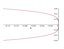
(a)

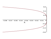
(b)

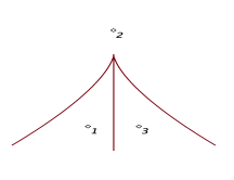
(c)

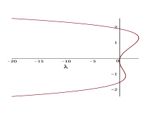
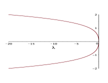
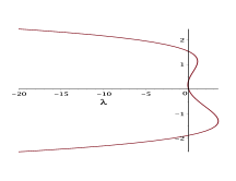
Figure 1: The vertical axes stand for the state variable $x.$ Diagrams 1(a) and 1(b) depict bifurcation diagrams of $g$ in Equation (2.3) and its normal form $f,$ respectively. The diagram 1(c) shows the transition set and the regions 1-3 associated with Equation (2.6). The second row illustrates the persistent bifurcation diagrams associated with these regions.

Real life problems can not be perfectly modeled by a system of equations and imperfections are always inevitable. Furthermore, the singularity of a germ $g$ implies that the zeros of a small perturbation of $g,$ say

$$h(x,\lambda,\beta)=0,\hbox{ where }h(x,\lambda,0)=g(x,\lambda),$$ (2.4)

may behave substantially different than what the zero structure associated with $g=0$ does. The parameterized germ $h$ in (2.4) is called an unfolding of $g.$ Hence, modeling imperfections and the possible existence of additional parameters in a model are the main obstacles of simply using normal forms of a singular germ for the qualitative understanding of a real life problem. Thus, the approach needs to be refined through the notion of universal unfolding. In fact, we are interested to find a parameterized family like

$$G(x,\lambda,\alpha)=0,\quad\alpha\in\mathbb{R}^{p},$$ (2.5)

such that for any small perturbation $\epsilon p(x,\lambda,\epsilon)$, the germ $g+\epsilon p(x,\lambda,\epsilon)$ would be contact-equivalent to $G(x,\lambda,\alpha(\epsilon))$ for some germ $\alpha(\epsilon).$ We call such germ $G$ a versal unfolding of $g.$ A versal unfolding with the minimum possible number of parameters is called a universal unfolding for $g$; see [29, Definitions 1.1 and 1.3, Pages 120–121] and [31, Definitions 6.4.2 and 6.4.3, Page 176]. The number of parameters in a universal unfolding is named the codimension of $g.$ The universal unfolding accommodates any possible modeling imperfections, any arbitrary small perturbation and also the existence of any possible number of parameters (in addition to the distinguished parameter $\lambda).$ In order to derive the universal unfolding of a given singularity, the computation of a vector space called tangent space or instead a basis for its complement is required. Using Singularity’s command ${\tt UniversalUnfolding(g,[x,\lambda],5,normalform)}$ for $g$ in (2.3) gives rise to

$$G(x,\lambda,\alpha_{1},\alpha_{2}):=x^{4}+\lambda+\alpha_{1}x+\alpha_{2}x^{2}.$$ (2.6)

Bifurcation diagram classification of the universal unfolding gives an insight to the zero structure of a germ and any of its perturbations. This is studied by the notion of persistence in the bifurcation diagrams. In fact a bifurcation diagram is called persistent when all its small perturbations remain self contact-equivalent, and otherwise it is called nonpersistent. Finding nonpersistent systems and their associated subset of the parameter space (the so-called transition set $\Sigma$) play a central role in this classification. More precisely, all parametric germs associated with parameters in a connected component of $\Sigma^{c},$ complement of $\Sigma,$ are contact-equivalent. Therefore by choosing a parameter from each connected component of $\Sigma^{c},$ a complete list of persistent bifurcation diagrams modulo contact-equivalent is obtained. The non-persistence may either originate from a local nature or be caused by the singular boundary conditions. Local nonpersistent bifurcation diagrams are determined with families of germs associated with three semi-algebraic parameter spaces of codimension one; i.e., bifurcation $\mathscr{B}$, hysteresis $\mathscr{H}$ and double limit point $\mathscr{D}$; see [29, Page 140] for details. Nonpersistent germs associated with boundary conditions add extra complications into the solution dynamics, when bifurcation diagrams cross the boundary; see [29, Pages 154–165]. Given our description for any finite codimension singularity, the connected components of the complement set of the transition set, i.e., $\Sigma^{c},$ provide the qualitative classification of persistent bifurcation diagrams. The command $\verb|TransitionSet|(G,[\alpha_{1},\alpha_{2}],[x,\lambda])$ for $G$ in (2.6) gives

$$\mathscr{B}:=\emptyset,\quad\mathscr{H}:=\{(\alpha_{1},\alpha_{2})\,|\,8\alpha_{2}^{3}=-27\alpha_{1}^{2}\},\quad\mathscr{D}:=\{(\alpha_{1},\alpha_{2})\,|\,\alpha_{1}=0,\alpha_{2}\leq 0\},$$

and $\Sigma:=\mathscr{H}\cup\mathscr{D}.$ The transition set $\Sigma$ is plotted in Figure 1(c). $\verb|PersistentDiagram|(G,[x,\lambda],\break\verb"plot",\verb"ShortList")$ plots a complete list including all contact-inequivalent types of persistent bifurcation diagrams for $G$; see the second row in Figure 1.

3 Ideal membership problem and tools from algebraic geometry

Given our description in the previous section, we mainly need to address the ideal membership problem in the ring of smooth germs. We call an ideal basis for the (finite) generators of a finitely generated ideal. The ideal membership problem refers to the question on whether or not an element belongs to a predefined ideal. Although a finitely generated ideal is defined by an ideal basis, yet it is not an easy task to understand whether a given element belongs to the ideal or not. There are two different ways to facilitate the ideal membership problem. One is to find a convenient ideal presentation from which the ideal membership can be easily understood. This is feasible for certain ideals and will be addressed in Section 5. The second is a computational approach based on a division algorithm. Dividing a given element by the ideal basis (generators), the element certainly belongs to the ideal when the remainder is zero. However for non-zero remainders with respect to an arbitrary ideal basis, the division may not help to conclude about the membership of the element in the ideal. B. Buchberger in 1965 introduced an ideal basis (called Gröbner basis) for ideals in the polynomial ring on which zero/nonzero remainders would indeed conclude the ideal membership; see [8, 7, 9, 6].

Armbruster and Kredel [2] suggested a cognitive use of Gröbner basis for computing universal unfolding; also see [1]. Then, Gatermann and Lauterbach [17] extended the tools for equivariant bifurcation problems. Wright and Cowel in [11] noticed that a local version of Gröbner basis is indeed the appropriate tool to work with it in this theory. In fact, naive uses of Gröbner basis yield wrong results for many singularities (e.g., see Example 4.2). The main reason is that Gröbner basis may work with polynomial germs, while the ring of smooth germs is a considerably larger ring than the polynomial germs. Recall that a set may generate a larger ideal in a ring than what it generates in a subring. Since Wright and Cowel’s remark, the only result in this direction is due to Gatermann and Hosten [18]. This is a fundamental contribution, but it is yet incomplete. They used (mixed) standard basis for “mixed modules” over fractional maps and multi-dimensional state variables. They discussed neither of Taylor series truncations, smooth maps and germs, nor computations with smooth maps of finite or infinite codimensions. Their algorithms are indeed useful for possible implementations in a computer algebra system to simplify certain fractional maps with finite codimension. Although they did not discuss their approach limitations, their suggested algorithms are limited to the cases when their associated (restricted) tangent space is a zero dimensional ideal in the ring of fractional (germs) maps. However, they are not yet sufficient to compute normal forms and the associated normalizing transformations. We further remark that any useful implementation of the results in a computer algebra system for their real life applications in bifurcation theory needs to treat arbitrary singular smooth maps. As far as our information is concerned, there does not yet exist any contribution to discuss on how to implement the results in bifurcation theory for actual bifurcation analysis of singularities; see Section 6 in this direction. Our suggested algorithms also provide a systematic approach for detection and treatment of infinite and high codimensional singularities and their possible persistent bifurcation diagram classifications.

The localization of the polynomial-germ ring gives rise to the fractional germs, i.e., germs with a fractional representative in their germ-equivalent class. Although the set of all fractional germs is a local ring, yet it is still a much smaller ring than the ring of smooth germs. The other alternative is the local germ ring of all formal power series. This is a larger ring than the fractional germs and it is, perhaps, suitable due to Borel lemma. Borel lemma indicates the existence of a one-to-one correspondence modulo flat functions between smooth germs and formal power series through their Taylor series expansion.

3.1 Standard and Gröbner bases for ideals

Let $K$ be a field of characteristic zero; in particular we are interested in the field of real numbers. For our convenience, we simply identify a given germ with a convenient representative of that germ. For instance, we talk about the polynomial germ ring over the field $K$ and denote it by $K[x,\alpha]$ while we mean the ring of all smooth germs whose germ-equivalent class have a polynomial representative. The quotient ring of $\mathscr{E}$ over the ideal of all flat germs is denoted by $K[[x,\alpha]]$ due to the fact that it is ring-isomorphic to the ring of formal power series. Thus, we call $K[[x,\alpha]]$ the germ ring of formal power series. Further, we identify members of $K[[x,\alpha]]$ with the infinite Taylor expansion of their representative. Since $K[x,\lambda]$ and $K[[x,\lambda]]$ are Noetherian rings, we can guarantee termination of most algorithms during the computations.

Denote $\deg(X^{\alpha}):=\alpha_{1}+\ldots+\alpha_{n}$ when $X^{\alpha}:=x_{1}^{\alpha_{1}}x_{2}^{\alpha_{2}}\cdots x_{n}^{\alpha_{n}},$ $X:=(x_{1},x_{2},\ldots,x_{n})$ and $\alpha:=(\alpha_{1},\alpha_{2},\ldots,\alpha_{n})\in Z_{\geq 0}^{n}.$ Any expression like $X^{\alpha}$ is called a monomial germ while a term in $\mathscr{E}$ means a monomial germ along with its coefficient. We define the lexicographic ordering $\prec_{{\rm lex}}$ on monomial germs $X^{\alpha}$ as follows:

$$X^{\alpha}\prec_{{\rm lex}}X^{\beta}\hbox{ when }\alpha_{i}-\beta_{i}\hbox{ is negative for }i:=\inf\{j\,|\,\alpha_{j}-\beta_{j}\neq 0\}.$$

Definition 3.1.

A local order $\prec$ is a total ordering (every two terms are comparable) and furthermore,

• For any $\alpha,\beta,\gamma\in Z_{\geq 0}^{n}$, the condition $X^{\alpha}\prec X^{\beta}$ implies $X^{\alpha+\gamma}\prec X^{\beta+\gamma}$.

• $x_{i}\prec 1$ for all $i=1,\ldots,n$. We further assume that $0\prec X^{\alpha}$ for any $\alpha.$

Due to Dickson’s lemma (see [4, Page 251] and [12, Page 71]), every (infinite) set of monomials have a maximum with respect to any arbitrary local order; here, the condition $X^{\beta}|X^{\alpha}$ implies $X^{\alpha}\preceq X^{\beta}.$ An important example of a local order is anti-graded lexicographic ordering $\prec_{{\rm alex}}$ defined by

$$X^{\alpha}\prec_{{\rm alex}}X^{\beta}\Leftrightarrow\left\{\begin{array}[]{lcl}\deg(X^{\alpha})>\deg(X^{\beta}),&&\\ &&\\ \deg(X^{\alpha})=\deg(X^{\beta})&\text{and}&X^{\alpha}\prec_{{\rm lex}}X^{\beta}.\end{array}\right.$$

The localization of the polynomial germ ring is defined as

$$\mathscr{R}:=\left\{\frac{f}{g}\mid f,g\in K[x,\lambda],g(0,0)\neq 0\right\}$$

whose unique maximal ideal is generated by $x$ and $\lambda.$ It is common to denote $\mathscr{R}$ with $K[x,\lambda]_{\langle x,\lambda\rangle}.$ We call $\mathscr{R}$ the ring of fractional germs. Throughout this paper, we denote

$$\mathcal{R}\hbox{ for either of the local rings }K[[x,\lambda]],\mathscr{R},\hbox{ or }\mathscr{E},$$

unless it is explicitly stated.

Definition 3.2.

Let $f\in\mathcal{R}$ and $\prec$ be a local order. The infinite jet and $k$-jet of $f$ are defined by its Taylor series expansion around the origin and denoted by

$$J^{\infty}(f):=\sum_{(i,j)}a_{ij}x^{i}\lambda^{j},\;\hbox{and }\;J^{k}(f):=\sum_{i+j\leq k}a_{ij}x^{i}\lambda^{j}\quad\hbox{ for }a_{ij}\in K.$$

The set of terms of $f$ are defined by

$${\rm Terms}(f):=\left\{a_{ij}x^{i}\lambda^{j}\,|\,a_{ij}\neq 0\right\},$$

i.e., all terms appearing in $J^{\infty}(f).$ When ${\rm Terms}(f)\neq\emptyset,$ the leading term of $f$ is

$${\mathrm{LT}}(f)=\max\,{\rm Terms}(f),$$

i.e., ${\mathrm{LT}}(f)\in{\rm Terms}(f)$ and $p\prec{\mathrm{LT}}(f)$ for any $p\in{\rm Terms}(f)\setminus\{{\mathrm{LT}}(f)\}.$ The germ $g$ is flat iff ${\rm Terms}(f)=\emptyset.$ We define ${\mathrm{LT}}(f):=0,$ when $f$ is a flat germ, i.e., $J^{\infty}(f)=0.$ The coefficient and monomial of the leading term are respectively called the leading coefficient (${\mathrm{LC}}$) and leading monomial (${\mathrm{LM}}$). For the case of $f\in K[x,\lambda]$ and $\prec_{{\rm lex}},$ we may similarly define ${\mathrm{LT}}(f),{\mathrm{LC}}(f)$ and ${\mathrm{LM}}(f).$

Now we present some definitions, terminologies and theorems from [13, 12, 32, 4]. These are suitably modified and generalized to fit in our purpose.

Definition 3.3 (Remainder).

A remainder of a germ $f$ with respect to the set of germs $G=\{g_{1},\ldots,g_{m}\}\subset\mathscr{E}$ and the local order $\prec$ is defined as a germ ${\rm Rem}(f,G,\prec)\in\mathscr{E}$ so that

• ${\rm Rem}(f,G,\prec)=f-\sum_{i=1}^{m}q_{i}g_{i}$, for some $q_{1},\ldots,q_{m}\in\mathscr{E}$ so that ${\mathrm{LT}}(q_{i}g_{i})\preceq{\mathrm{LT}}(f)$.

• No term of ${\rm Rem}(f,G,\prec)$ is divisible by any of ${\mathrm{LT}}(g_{i})$ for $i=1,\ldots,m$.

By replacing $\mathscr{E}$ with $K[[x,\lambda]]$ in Definition 3.3, the remainders in the ring of $K[[x,\lambda]]$ is readily defined; also see [4, Pages 251-252]. The same is true for the case of polynomial germ ring $K[x,\lambda]$ provided that the local order $\prec$ would be instead a monomial ordering like ${\prec_{{\rm lex}}}.$ The remainders in the ring of $\mathscr{R}$ is defined in [13, Page 170] using Mora normal form algorithm. Usually, the terminology of normal form is used rather than remainder. However, we choose remainder as the other may cause confusion with the normal forms of germs in singularity theory. The division here is related to Malgrange preparation theorem and Mather division theorem; see [38, Corollaries A.6.2 and A.7.2, Theorem A.7.1].

When $f$ is flat, its remainder with respect to any set of germs and local order is flat. The remainder is not necessarily unique even modulo flat germs; also see [4, Pages 251-252]. In fact, the remainder is unique modulo flat germs when $G$ is a standard basis (or Gröbner basis for the case of $K[x,\lambda]$), defined as follows.

For an ideal $I$ in $\mathcal{R},$ we define the leading term ideal ${\mathrm{LT}}(I)_{\mathcal{R}}$ by

$${\mathrm{LT}}(I)_{\mathcal{R}}:=\langle{\mathrm{LT}}(f):f\in I\rangle_{\mathcal{R}}.$$

Definition 3.4 (Standard basis).

Let $I$ be an ideal in $\mathcal{R}$ with a finite generating set $\{g_{1},\ldots,g_{m}\}\subset I$. The set $\{g_{1},\ldots,g_{m}\}$ is called a standard basis of $I$ when

$${\mathrm{LT}}(I)_{\mathcal{R}}=\langle{\mathrm{LT}}(g_{1}),\ldots,{\mathrm{LT}}(g_{m})\rangle_{\mathcal{R}}.$$ (3.1)

The set $\{g_{1},\ldots,g_{m}\}\subseteq\mathcal{R}$ is called a standard basis in $\mathcal{R}$ when it is a standard basis for the ideal $\langle g_{1},\ldots,g_{m}\rangle_{\mathcal{R}}$.

Remark 3.5.

• The set $\{g_{1},\ldots,g_{m}\}\subset K[x,\lambda]$ is called Gröbner basis with respect to $\prec_{{\rm lex}}$ when the condition (3.1) holds.

• Any finite set of germs $\{g_{i}\;|\;1\leq i\leq m\}$ in $\mathscr{E}$ is a standard basis in $\mathscr{E}$ iff the set of formal power series $\{J^{\infty}(g_{i})\}$ is a standard basis in $K[[x,\lambda]].$

• Let $\mathcal{R}:=K[x,\lambda],K[[x,\lambda]]$ or $\mathscr{R}$ and $\{g_{1},\ldots,g_{m}\}\subset I$ be a finite set. Then,

  $${\mathrm{LT}}(I)_{\mathcal{R}}=\langle{\mathrm{LT}}(g_{1}),\ldots,{\mathrm{LT}}(g_{m})\rangle_{\mathcal{R}}$$

  implies that $\{g_{1},\ldots,g_{m}\}\subset I$ is a generating set for $I$. This has a simple argument as follows; also see [3, Page 206]. For any $f\in I,$

  $$r:={\rm Rem}\big{(}f,\{g_{i}|\,i=1,\ldots,m\},\prec\big{)}\in I.$$

  Thus, ${\mathrm{LT}}(r)\in{\mathrm{LT}}(I)_{\mathcal{R}}$ and ${\mathrm{LT}}(r)$ must be factored by ${\mathrm{LT}}(g_{i})$ for some $i.$ The latter implies that $r=0,$ otherwise this contradicts with $r$ being a remainder.

Computation of standard basis uses the notion of $S$-germs. Let $f,g\in\mathcal{R}$ and $\preceq$ be a local order. Then, S-germ of $f$ and $g$ is defined by

$$S(f,g)=\left\{\begin{array}[]{lcl}\frac{{\mathrm{LCM}}\big{(}{\mathrm{LM}}(f),{\mathrm{LM}}(g)\big{)}}{{\mathrm{LT}}(f)}f-\frac{{\mathrm{LCM}}\big{(}{\mathrm{LM}}(f),{\mathrm{LM}}(g)\big{)}}{{\mathrm{LT}}(g)}g&\hbox{ if }&J^{\infty}(f)J^{\infty}(g)\neq 0,\\ 0&\hbox{ for }&J^{\infty}(f)J^{\infty}(g)=0.\end{array}\right.$$

Here ${\mathrm{LCM}}$ stands for the least common multiple for a pair of monomials.

Theorem 3.6.

(See [33], [20, Theorem 2.6], and Hironaka theorem on [4, Page 252]) Let $\mathcal{R}=\mathscr{E}$ or $K[[x,\lambda]]$, $G=\{g_{1},\ldots,g_{m}\}\subsetneq\mathcal{R},$ $0\neq f\in\mathcal{R}$ and $\prec$ be a local order. Then,

• Always $f$ has a remainder with respect to $\prec$ and $G.$

• The set $G$ is a standard basis iff the remainder of $f$ with respect to $G$ and $\prec$ is unique modulo flat germs.

• (Buchberger’s Criterion) The set $G=\{g_{1},\ldots,g_{m}\}$ is a standard basis iff for all $i,j,$ the expression ${\rm Rem}(S(g_{i},g_{j}),G,\prec)$ is a flat germ.

• The set $G$ is a standard basis iff ${\rm Rem}(f,G,\prec)$ is flat for all $f\in\langle G\rangle_{\mathcal{R}}$.

In order to compute the standard basis for an ideal in $K[[x,\lambda]]$ (and also in $\mathscr{E}$), one needs to sequentially enlarge and update its set of generators by only adding the non-flat remainders (with respect to the updated generators and a given local order) of the $S$-germs of the generator pairs. This process is usually known as Buchberger algorithm and it terminates when the ascending ideals generated by the leading terms of the updated generators stops any further enlargement. The Buchberger algorithm is finitely terminated due to the fact that $K[[x,\lambda]]$ is a Noetherian ring.

Example 3.7.

• The division of a polynomial by a set of polynomials in our division algorithm may involve formal power series; for example we have ${\rm Rem}(1,1-x,\prec_{{\rm alex}})=0=1-(\sum_{n=0}^{\infty}x^{n})(1-x).$

• The remainder of a polynomial divided by a polynomial may give rise to an infinite formal power series. For instance let $G:=\{x\lambda-x^{2}\lambda^{2}-x^{4}\}.$ Then,

  $$h := {\rm Rem}(x^{2}\lambda,G,\prec_{{\rm alex}})=x^{5}+x^{9}+2x^{13}+5x^{17}+14x^{21}+\ldots$$

  $$= x^{2}\lambda-\big{(}x+x^{2}\lambda+x^{5}+x^{3}\lambda^{2}+2x^{6}\lambda+x^{4}\lambda^{3}+\ldots\big{)}(x\lambda-x^{2}\lambda^{2}-x^{4}).$$

  Since the generator of an ideal with only one generator is always a standard basis, the remainder here is unique.

• This example is to show that a finite set of polynomial ideal basis in $\mathscr{E}$ may lead to a standard basis that includes non-polynomial germs. Let $G=\{f:=x\lambda-x^{2}\lambda^{2}-x^{4},g:=\lambda-x\lambda-x\lambda^{2}-x^{3}\}$. Then, $S(f,g)=x^{2}\lambda.$ It is easy to verify that $S=\{f,g,h\}$ is a standard basis, where $h$ is defined in part (b).

The first and second Buchberger criteria are applied for efficient computation of standard basis in Singularity. However, we will not discuss them in this paper.

Definition 3.8 (Reduced standard germ basis).

Let $G=\{g_{1},\ldots,g_{n}\}$ be a standard basis and ${\mathrm{LC}}(g_{i})=1$ for $i=1,\ldots,n.$ When

• ${\mathrm{LT}}(g_{i})\nmid p$ for all $p\in{\rm Terms}(g_{j})$, except for when $p={\mathrm{LT}}(g_{i})$ and $i=j$,

the set $G$ is called a reduced standard basis.

Given a local order $\prec$, [4, Theorem 2.1, Page 255] states that any ideal in $K[[x,\lambda]]$ has a unique reduced standard basis.

Theorem 3.9.

(See [20, Theorem 2.9]) With respect to any local order $\prec$, every finitely generated ideal $I\subseteq\mathscr{E}$ has a reduced standard basis. The standard basis is unique modulo flat germs.

The following Theorem along with [20, Equation (2.2)] and Buchberger algorithm provide computational guidelines on how to compute a reduced standard basis in $\mathscr{E}.$

Theorem 3.10.

(See [4, Page 255] and [20, Theorem 2.10]) Let $I=\langle f_{1},\ldots,f_{n}\rangle_{\mathscr{E}}$.

• There always exist germs $g_{1},\ldots,g_{m}\in\mathscr{E}$ for $m\leq n$ so that

  $$I=\langle g_{1},\ldots,g_{m}\rangle_{\mathscr{E}}$$ (3.2)

  and ${\mathrm{LT}}(g_{i})\nmid p$ for all $p\in{\rm Terms}(g_{j})$, except for when $i=j$ and $p={\mathrm{LT}}(g_{i})$.

• Furthermore, assume that $\{f_{i}\}^{n}_{i=1}$ is a standard basis in $\mathscr{E}.$ Then, the set $\{g_{i}\}^{m}_{i=1}$ (for $m\leq n$) can be chosen so that it is a reduced standard basis.

Example 3.11.

Let $f$ be a non-zero flat germ, and $I=\langle G\rangle_{\mathscr{E}}$ where

$$G:=\big{\{}g_{1}:=\lambda-\lambda\exp(x),g_{2}:=x-\sin(x),g_{3}:=\lambda x+\lambda^{3}+\lambda^{2}\ln(1+x)+f\big{\}}.$$

Since ${\mathrm{LT}}(G)=\{\lambda x,x^{3}\}$ and ${\mathrm{LT}}(I)=\langle\lambda x,x^{3},\lambda^{3}\rangle_{\mathscr{E}}$, $G$ is not a standard basis with respect to $\prec_{{\rm alex}}$. Due to

$${\rm Rem}\big{(}S(g_{1},g_{2}),G,\prec_{{\rm alex}}\big{)}=0,\quad{\rm Rem}\big{(}S(g_{2},g_{3}),G,\prec_{{\rm alex}}\big{)}=-x^{2}f$$

and ${\rm Rem}(S(g_{1},g_{3}),G,\prec_{{\rm alex}})=\lambda^{3}+f$, we add $\lambda^{3}+f$ to the basis, i.e., $S_{1}:=\{g_{1},g_{2},g_{3},\lambda^{3}+f\}$. Now $S_{1}$ is a standard basis, yet it is not a reduced standard basis. Given Theorem 3.10 and its proof,

$${\mathrm{LT}}(g_{1})\mid{\mathrm{LT}}(g_{3}),\quad{\rm Rem}\big{(}g_{3},S_{1}\setminus\{g_{3}\},\prec_{{\rm alex}}\big{)}=0,\quad S_{2}:=\{g_{1},g_{2},\lambda^{3}+f\}\hbox{ and }$$

$${\rm Rem}\big{(}\lambda x+g_{1},S_{2},\prec_{{\rm alex}}\big{)}={\rm Rem}\big{(}g_{2}-\frac{x^{3}}{6},S_{2},\prec_{{\rm alex}}\big{)}=0,$$

we define

$$S_{3}:=\{\lambda x,x^{3},\lambda^{3}+f\}.$$

Now $S_{3}$ is a reduced standard basis.

3.2 Finite codimension

Finite codimensional ideals demonstrate an important role in ideal presentation in Subsection 5. Let $\mathcal{M}_{\mathscr{E}}:=\langle x,\lambda\rangle_{\mathscr{E}}$, $\mathcal{M}_{\mathscr{R}}=\langle x,\lambda\rangle_{\mathscr{R}},$ $\mathcal{M}_{K[[x,\lambda]]}=\langle x,\lambda\rangle_{K[[x,\lambda]]},$ and $\mathcal{M}_{K[x,\lambda]}=\langle x,\lambda\rangle_{K[x,\lambda]}$.

Definition 3.12.

An ideal $I$ in $\mathscr{E}$ (or in $\mathscr{R},$ $K[[x,\lambda]]$) is said to have a finite codimension when ${\mathcal{M}_{\mathscr{E}}}^{k}\subseteq I$ (${\mathcal{M}_{\mathscr{R}}}^{k}\subseteq I,{\mathcal{M}_{K[[x,\lambda]]}}^{k}\subseteq I$) for $k\in\mathbb{N}.$ Equivalently, $I$ has a complement (vector) subspace in $\mathscr{E}$ with finite dimension.

Now we compare the ideals in $K[x,\lambda]$ with those in $\mathscr{R},$ $K[[x,\lambda]]$ and $\mathscr{E}.$

Theorem 3.13.

(See [20, Theorem 2.13]) Let $I$ be a finite codimensional ideal in $\mathscr{E}.$

• The ideal $I$ has a unique reduced standard polynomial germ basis.

• Assume that $G:=\{g_{i}\}^{n}_{i=1}$ is a standard basis for $I$ and $f\in\mathscr{E}.$ Then, the remainder is always a polynomial germ, i.e., ${\rm Rem}(f,G,\prec_{{\rm alex}})\in K[x,\lambda].$ In particular, we have $\deg({\rm Rem}(f,G,\prec_{{\rm alex}}))\leq k$ when ${\mathcal{M}_{\mathscr{E}}}^{k+1}\subseteq I.$

Example 3.14.

Let $S=\{f_{i}\}^{n}_{i=1}$ be a reduced standard basis whose generated ideal is of finite codimension. Then, ${\rm Rem}(f,S,\prec_{{\rm alex}})=f-\sum q_{i}f_{i}\in K[x,\lambda].$ However, $q_{i}$ may not always be a polynomial germ. Consider the ordering $\lambda\prec_{{\rm alex}}x$ and define

$$I:=\left\langle g_{1}:=2\lambda^{3}-3\lambda^{2}x+x^{5},g_{2}:=-3x\lambda^{2}+5x^{5},g_{3}:=-3\lambda^{3}+5x^{4}\lambda\right\rangle.$$ (3.3)

The ideal $I$ is finite codimensional since ${\mathcal{M}_{\mathscr{E}}}^{6}\subset I.$ Here, $G=\left\{g_{1},g_{2},g_{3},\frac{4}{3}x^{5}-\frac{10}{9}x^{4}\lambda\right\}$ is a standard basis and

$$S=\left\{f_{1}:=x\lambda^{2}-\frac{25}{18}x^{4}\lambda,f_{2}:=-\frac{1}{3}g_{3},f_{3}:=x^{5}-\frac{5}{6}x^{4}\lambda\right\}$$

is a reduced standard basis. Now we have

$$x^{3}\lambda^{3}=x^{3}f_{2}+\frac{25}{18}x^{5}qf_{1}+\frac{5}{3}\lambda x^{2}qf_{3},$$

where $q:=\sum^{\infty}_{i=0}(\frac{125}{108})^{i}x^{2i}$, ${\rm Rem}(x^{3}\lambda^{3},S,\prec_{{\rm alex}})=0$ while $q_{1}:=\frac{25}{18}x^{5}q$ and $q_{2}:=\frac{5}{3}\lambda x^{2}q$ are not polynomial germs.

The following theorem enables us to compute the standard basis for ideals in $\mathscr{E}$ through computations in the fractional germs.

Theorem 3.15.

Consider $I=\langle p_{1},\ldots,p_{n}\rangle_{\mathscr{E}},$ $\prec_{{\rm alex}}$ and ${\mathcal{M}_{\mathscr{R}}}^{k}\subseteq\langle p_{1},\ldots,p_{n}\rangle_{\mathscr{R}}\subseteq\mathscr{R}.$ Further, suppose that $\{q_{1},\ldots,q_{m}\}$ is a standard basis for $\langle p_{1},\ldots,p_{n}\rangle_{\mathscr{R}}.$ Then, $\{q_{1},\ldots,q_{m}\}$ is a standard basis for $I$.

Proof.

Let $g\in LT_{\mathscr{E}}(I)=\langle LT(f)\,|\,f\in I\rangle_{\mathscr{E}}.$ Since ${\mathcal{M}_{\mathscr{R}}}^{k}\subseteq\langle p_{1},\ldots,p_{n}\rangle_{\mathscr{R}},$ part (1) in Theorem 4.1 implies that ${\mathcal{M}_{\mathscr{E}}}^{k}\subseteq I$ and ${\mathcal{M}_{\mathscr{E}}}^{k}\subseteq LT_{\mathscr{E}}(I).$ Hence, without loss of generality we may assume that $g=J^{k}(g).$ Thus,

$$g=\sum a_{i}LT(f_{i})=J^{k}\sum a_{i}LT(f_{i})=\sum J^{k}(a_{i})LT(f_{i})+r,$$

where $a_{i}\in\mathscr{E},f_{i}\in I$ and $r\in{\mathcal{M}_{\mathscr{E}}}^{k+1}.$ Now we only need to prove that $LT(f_{i})\in\langle LT(q_{j}),j=1,\ldots m\rangle_{\mathscr{E}}$ when $\deg(LT(f_{i}))\leq k.$

Since $f_{i}\in I=\langle q_{j},j=1,\ldots m\rangle_{\mathscr{E}},$ $f_{i}=\sum b_{ij}q_{j}$ for some $b_{ij}\in\mathscr{E}.$ Thus,

$$J^{k}(f_{i})=J^{k}\sum J^{k}(b_{ij})q_{j}=\sum J^{k}(b_{ij})q_{j}+s$$

where $s\in{\mathcal{M}_{\mathscr{R}}}^{k+1}.$ Therefore, $J^{k}(f_{i})\in\langle q_{j},j=1,\ldots m\rangle_{\mathscr{R}}.$ On the other hand,

$$LT(f_{i})=LT(J^{k}(f_{i})) \in LT_{\mathscr{R}}\langle q_{1},\ldots,q_{m}\rangle_{\mathscr{R}}=\langle LT(q_{1}),\ldots,LT(q_{m})\rangle_{\mathscr{R}}$$

$$\subseteq \langle LT(q_{1}),\ldots,LT(q_{m})\rangle_{\mathscr{E}}.$$

This completes the proof. ∎

4 Truncation degree and alternative ring computations

One of the main obstacles in working with the local rings is termination of the algorithms. There are methods in the literature for computing the standard basis (for fractional maps using Mora normal form) so that they solve the problem of algorithm terminations. Yet for the case of formal power series, no computer program can compute and store infinite formal power series expansions and thus, their truncations up to certain degrees are mostly unavoidable. In order to circumvent this problem, we provide rigorous criteria so that the computations can be performed modulo a sufficiently high degree; see Theorem 4.3 (part 1). Further, we investigate and compare the computations in the local (germ) rings of polynomials, the fractional germs and formal power series with those in the ring of smooth germs. We discuss the circumstances on which they can be alternatively used. This helps to efficiently use the different algorithms and yet ensure about correctness of the results.

The following theorems are two of our main contributions in this paper and provide important alternatives and criteria for our computations in different circumstances including ideals with infinite codimension.

Theorem 4.1.

• Suppose that $G:=\{g_{1},\ldots,g_{n}\}\subset\mathscr{R}.$ Then, the ideal $\langle g_{1},\ldots,g_{n}\rangle_{\mathscr{E}}$ has a finite codimension iff $\langle g_{1},\ldots,g_{n}\rangle_{\mathscr{R}}$ is a finite codimension ideal. Assuming that $\langle g_{1},\ldots,g_{n}\rangle_{\mathscr{R}}$ has a finite codimension, for nonnegative integers $i$ and $j$, ${\mathcal{M}_{\mathscr{E}}}^{i}\langle\lambda^{j}\rangle_{\mathscr{E}}\subseteq\langle g_{1},\ldots,g_{n}\rangle_{\mathscr{E}}$ iff ${\mathcal{M}_{\mathscr{R}}}^{i}\langle\lambda^{j}\rangle_{\mathscr{R}}\subseteq\langle g_{1},\ldots,g_{n}\rangle_{\mathscr{R}}.$

• Let ${\mathcal{M}_{K[x,\lambda]}}^{k}\subseteq\langle g_{1},\ldots,g_{n}\rangle_{K[x,\lambda]}\subseteq K[x,\lambda].$ Then, ${\mathcal{M}_{K[x,\lambda]}}^{i}\langle\lambda^{j}\rangle_{K[x,\lambda]}\subseteq\langle g_{1},\ldots,g_{n}\rangle_{K[x,\lambda]}$ iff ${\mathcal{M}_{\mathscr{E}}}^{i}\langle\lambda^{j}\rangle_{\mathscr{E}}\subseteq\langle g_{1},\ldots,g_{n}\rangle_{\mathscr{E}}.$

• For a finite codimension ideal $\langle g_{1},\ldots,g_{n}\rangle_{\mathscr{R}}$ in $\mathscr{R}$ and an ideal $I$ in $\mathscr{E},$

  $$I=\langle g_{1},\ldots,g_{n}\rangle_{\mathscr{E}}\quad\hbox{ iff }\quad I\cap\mathscr{R}=\langle g_{1},\ldots,g_{n}\rangle_{\mathscr{R}}.$$

  In particular, let $I,J$ be two ideals in $\mathscr{E},$ $I$ have a finite codimension and $I\cap\mathscr{R}=J\cap\mathscr{R}.$ Then, $I=J.$

• For an ideal $I$ in $\mathscr{E},$ the following three conditions are equivalent.

  $${\hbox{ (i)}}\;\;{\mathcal{M}_{\mathscr{E}}}^{k}\subseteq I,\qquad{\hbox{ (ii)}}\;\;{\mathcal{M}_{\mathscr{R}}}^{k}\subseteq I\cap\mathscr{R},\qquad{\hbox{ (iii)}}\;\;{\mathcal{M}_{K[x,\lambda]}}^{k}\subseteq I\cap K[x,\lambda].$$

Proof.

Part (1). The if part is trivial. Thus, we assume that ${\mathcal{M}_{\mathscr{E}}}^{k}\subseteq\langle g_{1},\ldots,g_{n}\rangle_{\mathscr{E}}$ and prove that ${\mathcal{M}_{\mathscr{R}}}^{k}\subseteq\langle g_{1},\ldots,g_{n}\rangle_{\mathscr{R}}$. Using Nakayama lemma [29, Lemma 5.3, Page 71], it is enough to verify that ${\mathcal{M}_{\mathscr{R}}}^{k}\subset\langle g_{1},\ldots,g_{n}\rangle_{\mathscr{R}}+{\mathcal{M}_{\mathscr{R}}}^{k+1}$. Since ${\mathcal{M}_{\mathscr{E}}}^{k}\subset\langle g_{1},\ldots,g_{n}\rangle_{\mathscr{E}}$, for some $a_{s}\in\mathscr{E}$ we have

$$x^{l}\lambda^{k-l} = \sum_{s=1}^{n}a_{s}g_{s}=J^{k}\sum_{s=1}^{n}a_{s}g_{s}=\sum_{s=1}^{n}J^{k}\left(J^{k}(a_{s})g_{s}\right)=J^{k}\sum_{s=1}^{n}b_{s}g_{s}=\sum_{s=1}^{n}b_{s}g_{s}+r,$$

where $a_{s}\in\mathscr{E},b_{s}:=J^{k}(a_{s})$ and $r\in{\mathcal{M}_{\mathscr{R}}}^{k+1}.$ For the second claim, we do not need Nakayama lemma. We assume that ${\mathcal{M}_{\mathscr{R}}}^{k}\subseteq\langle g_{1},\ldots,g_{n}\rangle_{\mathscr{R}}.$ Similar to above, for $i+j<k$ we have $x^{l}\lambda^{i+j-l}=J^{k-1}(x^{l}\lambda^{i+j-l})=\sum_{s=1}^{n}b_{s}g_{s}+r,$ where $r\in{\mathcal{M}_{\mathscr{R}}}^{k}$ and $b_{s}\in\mathscr{R}.$

Part (2). Proof is similar to the proof of the second claim in part (1).

Part (3). Assume that $I=\langle g_{1},\ldots,g_{n}\rangle_{\mathscr{E}}.$ Trivially,

$$\langle g_{1},\ldots,g_{n}\rangle_{\mathscr{R}}\subseteq I\cap\langle g_{1},\ldots,g_{n}\rangle_{\mathscr{R}}.$$

Let $f\in I\cap\mathscr{R}.$ Thus, $f=\sum a_{i}g_{i}$ for some $a_{i}\in\mathscr{E}.$ So, $f=J^{k}\sum J^{k}(a_{i})g_{i}+h$ for an $h\in{\mathcal{M}_{K[x,\lambda]}}^{k+1}.$ Since the left hand side belongs to $\langle g_{1},\ldots,g_{n}\rangle_{\mathscr{R}},$ the proof of the if part is complete. Now assume that $I\cap\mathscr{R}=\langle g_{1},\ldots,g_{n}\rangle_{\mathscr{R}}$ and $f\in I.$ By part (1) and $\langle g_{1},\ldots,g_{n}\rangle_{\mathscr{E}}\subseteq I,$ $J^{k}(f)\in I$ for some $k\in\mathbb{N}.$ Since $J^{k}(f)\in I\cap\mathscr{R},$

$$J^{k}(f)=\sum a_{i}g_{i},\hbox{ for }a_{i}\in\mathscr{R}.$$

On the other hand $f-J^{k}(f)\in\langle g_{1},\ldots,g_{n}\rangle_{\mathscr{E}}.$ This completes the proof of part (3). Part (4) is trivial. ∎

The hypothesis of part (1) in Theorem 4.1 allows us to use fractional germs for computations while the condition in part (2) permits the use of Gröbner basis for our purposes despite the local nature of our results.

Example 4.2.

Part (1) from the previous theorem is not valid when $\mathscr{R}$ is replaced with $K[x,\lambda]$. For instance, consider the example given in [36, Table 1, III.1 for $k=5$] and [29, Page 77],

$$I:=\langle g_{1}:=x^{5}+x^{3}\lambda+\lambda^{2},g_{2}:=5x^{5}+3x^{3}\lambda,g_{3}:=5x^{4}\lambda+3x^{2}\lambda^{2}\rangle_{\mathscr{E}}.$$

The ideal $I$ has a finite codimension since ${\mathcal{M}_{\mathscr{E}}}^{6}\subset I$. However, the ideal $I_{0}:=\langle g_{1},g_{2},g_{3}\rangle_{K[x,\lambda]}$ has an infinite codimension in $K[x,\lambda]$. The reason for this is as follows. The reduced Gröbner basis of $I$ with respect to $\lambda\prec_{{\rm lex}}x$ is given by

$$G:=\big{\{}3125\lambda^{3}+108\lambda^{4},18\lambda^{3}+125\lambda^{2}x,2x^{3}\lambda+5\lambda^{2},2x^{5}-3\lambda^{2}\big{\}}.$$

Further for any natural number $n\geq 3,$ the remainder ${\rm Rem}(x^{n},G,\prec_{{\rm lex}})=c\lambda^{3}$ where $c\in K.$ Therefore, $x^{n}$ does not belong to $I_{0}$ and $I_{0}$ is an infinite codimensional ideal.

Theorem 4.3.

• Let $g_{1},\ldots,g_{n}\in\mathscr{E}$ and $k\leqslant N,$ for $k,N\in\mathbb{N}.$ Then,

  • Either of the conditions

    $${\mathcal{M}_{\mathscr{R}}}^{k}\subseteq\langle J^{N}g_{1},\ldots,J^{N}g_{n}\rangle_{\mathscr{R}}\;\;\hbox{ and }\;\;{\mathcal{M}_{K[[x,\lambda]]}}^{k}\subseteq\langle J^{N}g_{1},\ldots,J^{N}g_{n}\rangle_{K[[x,\lambda]]},$$

    is equivalent to ${{\mathcal{M}_{\mathscr{E}}}}^{k}\subseteq\langle g_{1},\ldots,g_{n}\rangle_{\mathscr{E}}.$

  • If ${\mathcal{M}_{K[x,\lambda]}}^{k}\subseteq\langle J^{N}g_{1},\ldots,J^{N}g_{n}\rangle_{K[x,\lambda]}\subseteq K[x,\lambda].$ Then,

    $${\mathcal{M}_{K[x,\lambda]}}^{i}\langle\lambda^{j}\rangle_{K[x,\lambda]}\subseteq\langle J^{N}g_{1},\ldots,J^{N}g_{n}\rangle_{K[x,\lambda]}\;\;\hbox{ iff }\;\;{\mathcal{M}_{\mathscr{E}}}^{i}\langle\lambda^{j}\rangle_{\mathscr{E}}\subseteq\langle g_{1},\ldots,g_{n}\rangle_{\mathscr{E}}.$$

• Consider the finite sequence of nonnegative integers $k_{i},l_{i}\in\mathbb{N}$ so that the sequence $k_{i}+l_{i}$ is decreasing and $l_{i}$ is increasing. Let $\langle f_{1},f_{2},\ldots,f_{n}\rangle_{\mathscr{E}}$ be an ideal that is not necessarily of finite codimension and

  $$I:=\sum{\mathcal{M}_{\mathscr{R}}}^{k_{i}}\langle\lambda^{l_{i}}\rangle_{\mathscr{R}}\subseteq\langle J^{N}f_{1},\ldots,J^{N}f_{n}\rangle_{\mathscr{R}}.$$ (4.1)

  Then, either of the following conditions

  • for each $j\leq n,$ ${\rm Terms}(f_{j}-J^{p_{j}}f_{j})\subseteq\mathcal{M}_{\mathscr{R}}I$ for some $p_{j}\leq N.$

  • for each $j\leq n,$ $f_{j}\in\mathscr{R}$ and $f_{j}-J^{p_{j}}f_{j}\in\mathcal{M}_{\mathscr{R}}I$ for some $p_{j}\leq N.$

  implies that

  $$\sum{\mathcal{M}_{\mathscr{E}}}^{k_{i}}\langle\lambda^{l_{i}}\rangle_{\mathscr{E}}\subseteq\langle f_{1},f_{2},\ldots,f_{n}\rangle_{\mathscr{E}}.$$ (4.2)

Proof.

Part (1). Now the assumption ${\mathcal{M}_{\mathscr{R}}}^{k}\subset\langle J^{N}g_{1},\ldots,J^{N}g_{n}\rangle_{\mathscr{R}}$ implies that for some $a_{i}\in\mathscr{R},$ and any $i=1,\ldots k,$

$$x^{k-i}\lambda^{i}=J^{k}\sum_{i=1}^{n}a_{i}J^{N}(g_{i})=J^{k}\sum_{i=1}^{n}a_{i}g_{i}=\sum_{i=1}^{n}a_{i}g_{i}+r,\quad\hbox{ for }\quad k\leqslant N,$$

where $r\in{\mathcal{M}_{\mathscr{R}}}^{k+1}$. This and Nakayama lemma conclude that ${{\mathcal{M}_{\mathscr{E}}}}^{k}\subseteq\langle g_{1},\ldots,g_{n}\rangle_{\mathscr{E}}$. The converse and rest of the proof use similar arguments. Note that Nakayama lemma given in [29, Lemma 5.3] is also true when $\mathscr{E}$ is replaced with $\mathscr{R}$ and $K[[x,\lambda]].$

By the first part and ${\mathcal{M}_{K[x,\lambda]}}^{k}\subseteq\langle J^{N}g_{1},\ldots,J^{N}g_{n}\rangle_{K[x,\lambda]}$, we have ${\mathcal{M}_{\mathscr{E}}}^{k}\subseteq\langle g_{1},\ldots,g_{n}\rangle_{\mathscr{E}}$ and $\langle g_{1},\ldots,g_{n}\rangle_{\mathscr{E}}=\langle J^{N}g_{1},\ldots,J^{N}g_{n}\rangle_{\mathscr{E}}$. The rest of the proof is complete by Theorem 4.1(2).

Since ${\mathcal{M}_{\mathscr{E}}}^{i}\langle\lambda^{j}\rangle_{\mathscr{E}}\subset\langle g_{1},\ldots,g_{n}\rangle_{\mathscr{E}}$, for some $a_{s}\in\mathscr{E}$ we have

$$x^{l}\lambda^{i+j-l} = \sum_{s=1}^{n}a_{s}g_{s}=J^{k-1}\sum_{s=1}^{n}a_{s}g_{s}=\sum_{s=1}^{n}J^{k-1}\left(J^{k-1}(a_{s})J^{N}(g_{s})\right)=J^{k-1}\sum_{s=1}^{n}b_{s}J^{N}(g_{s})$$

$$= \sum_{s=1}^{n}b_{s}J^{N}(g_{s})+r,$$

where $b_{s}:=J^{k-1}(a_{s})$ and $r\in{\mathcal{M}_{K[x,\lambda]}}^{k}.$ Since ${\mathcal{M}_{K[x,\lambda]}}^{k}\subseteq\langle J^{N}g_{1},\ldots,J^{N}g_{n}\rangle_{K[x,\lambda]}$, from the above equality one can conclude ${\mathcal{M}_{K[x,\lambda]}}^{i}\langle\lambda^{j}\rangle_{K[x,\lambda]}\subseteq\langle J^{N}g_{1},\ldots,J^{N}g_{n}\rangle_{K[x,\lambda]}$.

Part (2) is concluded by Nakayama lemma and the fact that

$$x^{k_{i}-m}\lambda^{l_{i}+m}=\sum a_{i}J^{N}f_{i}=\sum a_{i}f_{i}+r,$$

where

$$r\in\langle{\rm Terms}(f_{j}-J^{N}f_{j})\rangle_{\mathscr{R}}\subseteq\langle{\rm Terms}(f_{j}-J^{p_{j}}f_{j})\rangle_{\mathscr{R}}\subset\mathcal{M}_{\mathscr{R}}I.$$

∎

4.1 Computation

The following items (I)-(XVI) provide our suggested algorithms that they are required for symbolic implementation of the results in a computer algebra system.

1. Truncation degree and computational rings for ideals

   Depending on the type of input germs, our computations can be converted from $\mathscr{E}$ to alternative smaller rings. This is feasible via Theorems 4.1 and 4.3. Now suppose that we are given an ideal $\langle g_{1},\ldots,g_{n}\rangle_{\mathscr{E}}$ with $g_{1},\ldots,g_{n}\in\mathscr{E}$. By multiplication matrix approach and standard basis computation, we can verify if the hypothesis of any part in Theorems 4.1 and 4.3 holds. In fact, from Theorem 4.3$(1)$ we find the permission for converting our computational ring to either of $\mathscr{R}$, $K[[x,\lambda]]$, or $K[x,\lambda]$. For when $g_{1},\ldots,g_{n}\in\mathscr{R}$, computations are converted to the computational rings $\mathscr{R}$ and/or $K[x,\lambda]$ when part $(1)$ and/or $(2)$ in Theorem 4.1 holds, respectively. In the case that $\langle g_{1},\ldots,g_{n}\rangle_{\mathscr{E}}$ is not a finite codimensional ideal, we resort to Theorem 4.3$(2)$. These arguments give rise to the following procedure:

   Procedure 4.4.

   For the output computations regarding the ideal $\langle g_{1},\ldots,g_{n}\rangle_{\mathscr{E}}$ when

   1. The inputs $g_{1},\ldots,g_{n}\in\mathscr{E}$, we have

      1. Theorem 4.3(1) holds for $k\leq 20$, return $k$ as truncation degree and $K[x,\lambda]$, $\mathscr{R}$, $K[[x,\lambda]]$, $\mathscr{E}$ as permissible computational rings.

      2. Theorem 4.3(1)(a) holds and 4.3(1)(b) fails for $k\leq 20$, we return $k$ as truncation degree and $\mathscr{R}$, $K[[x,\lambda]]$, $\mathscr{E}$ as permissible computational rings.

      3. Theorem 4.3(1) fails for $k\leq 20$, the only permissible computational ring is $\mathscr{E}$ and no clear truncation degree is available. Yet Theorem 4.3(2) provides a procedure for finding permissible truncation degree and the corresponding computational ring as $\mathscr{R}$ for computation of the intrinsic part of the ideal $\langle g_{1},\ldots,g_{n}\rangle_{\mathscr{E}}$.

   2. The inputs $g_{1},\ldots,g_{n}\in K[x,\lambda]$, we have

      1. Theorem 4.1(1)-(2) hold. Then, return $K[x,\lambda]$, $\mathscr{R}$, $\mathscr{E}$ as permissible computational rings and the maximal number $k$ in part (2) is the permissible truncation degree.

      2. Theorem 4.1(1) holds, i.e.,

         $$\exists\,\,{\mathcal{M}_{\mathscr{R}}}^{k}\subseteq\langle g_{1},\ldots,g_{n}\rangle_{\mathscr{R}}\quad\hbox{and}\quad k\leq 20.$$ (4.3)

         and 4.1(2) fails for $k$. In this case, the only permissible computational rings are $\mathscr{R}$ and $\mathscr{E}$ while minimal number $k$ in Equation (4.3) represents the permissible truncation degree.

      3. Theorem 4.1(1)-(2) fail. Since the inputs are polynomials, the truncation is not needed. Hence, the number $N$ in Equation (4.1) is taken as the Singularity’s default upper bound $N=20$ or the alternative choice given by the informative user.

   enumerate

   Remark 4.5.

   When the codimension of a singular germ is too large or infinity, our algorithms need an upper bound for termination of computations. Therefore, the default upper bound for computation of a singular germ is set to be 20. The truncation degree option in each procedure provides our users to increase or decrease this default number; see [19] for further details.

   enumerate[[(I)]]

2. Truncation degree and computational rings for a smooth germ

   For computations regarding a singular germ when there is no specified input data from the user, there is a necessity for an algorithmic derivation of suitable truncation degree and computational rings. This procedure is given as follows.

   Procedure 4.6.

   For an input germ $g\in\mathscr{E}$ and the required output truncation degree $k$ and computational ring $\mathcal{R}$:

   • Define the ideal $I(g):=\langle xg,\lambda g,x^{2}g_{x},\lambda g_{x}\rangle_{\mathscr{E}}$; compare $I(g)$ with the high order term ideal defined by equation (6.1). Next, follow the procedure 4.4 to find the truncation degree $k$ and computational ring $\mathcal{R}$ for the ideal $I(g)$. Return $k$ and $\mathcal{R}.$

3. Remainder

   General smooth inputs (not necessarily polynomials) indeed are important for many applications in the modeling and analysis of real life problems. Division algorithms in computers for general computational rings $\mathscr{E}$ and $K[[x,\lambda]]$ seem impractical in general. In this regard, our implementation of division algorithm for its applications in bifurcation theory is feasible given Definition 3.3, Theorems 3.13–4.3), and in particular Procedures 4.4–4.6. This is one of our claimed novel contributions in this paper. Division algorithm computation of a smooth germ $g$ divided by a set of smooth germs $\{f_{1},\ldots,f_{n}\}$ for the remainder is a fundamental tool in Singularity. Our implementation adapts the algorithms based on three computational rings $\mathscr{R}$, $K[[x,\lambda]]$ and $\mathscr{E}$. The inputs $g$ and $\{f_{1},\ldots,f_{n}\}$ can be arbitrarily chosen from either of these rings. The division algorithm in $\mathscr{R}$ is known as Mora normal form [13, Page 170].

4. Standard Bases

   Standard bases are the basis of most computations in Singularity in four computational rings $K[x,\lambda]$, $\mathscr{R}$, $K[[x,\lambda]]$, and $\mathscr{E}$; see Definitions 3.4 and 3.8, and Theorems 3.6, 3.9, 3.10, 3.13(1), 3.15, 4.1, 4.3.

   5 Intrinsic ideal representation

   An elegant approach for answering the ideal membership problem is to provide a good presentation for ideals. In this section we define intrinsic ideals and use it for such representation. This plays a central role in developing Singularity and is a prerequisite for most computations of objects presented in Section 6.

   Definition 5.1.

   When only the trivial reparametrization $\Lambda(\lambda)=\lambda$ is allowed in Equation (2.2), the associated relation $\thicksim_{s}$ is called strongly equivalent relation; see [29, Page 51]. Then, an ideal $I$ is called intrinsic [29, Page 81] when $I$ includes all strongly equivalent classes of its members.

   By [29, Proposition 7.1], every finite codimension ideal $I$ in $\mathscr{E}$ is intrinsic if and only if there exist nonnegative integers $s,m_{i},n_{i}$ for $i=0,\ldots,s$ so that

   $$I=\sum^{s}_{i=0}{\mathcal{M}_{\mathscr{E}}}^{m_{i}}\langle\lambda^{n_{i}}\rangle_{\mathscr{E}},$$ (5.1)

   $n_{0}=0,$ and the sequence $n_{i}$ is strictly increasing while $m_{i}+n_{i}$ is strictly decreasing. The conditions on $m_{i}$ and $n_{i}$ make the representation (5.1) unique. Equation (5.1) for intrinsic ideals gives a convenient answer for the ideal membership problem. The monomials $x^{m_{i}}\lambda^{n_{i}}$ for $i=0,\ldots,s$ are called intrinsic generators of the intrinsic ideal $I.$ For non-intrinsic ideals or more generally for a vector space $I,$ we define their intrinsic part; i.e., we denote ${\rm Itr}(I)$ for the largest intrinsic ideal contained in $I$.

   Lemma 5.2.

   For an intrinsic ideal $I$, there always exists a reduced monomial standard basis for $I$ that includes its intrinsic generators. Let $I$ be a finite codimension vector subspace of $\mathscr{E}$ or be a finitely generated ideal. Then, there exist nonnegative integers $m$ and $n,$ a reduced monomial standard basis $\{f_{j}\}^{n}_{j=1}$ for ${\rm Itr}(I)$ and $\{g_{i}\}^{m}_{i=1}\subset\mathscr{E}$ so that

   $$I={\rm Itr}(I)+\langle\{g_{i}\}^{m}_{i=1}\rangle_{\mathcal{R}},$$ (5.2)

   where $\mathcal{R}:=\mathscr{E}$ or $\mathcal{R}:=K.$ Here, none of the terms in ${\rm Terms}(g_{i})$ is divisible by $f_{j},$ i.e., ${\rm Itr}(I)\cap(\cup^{m}_{i=0}{\rm Terms}(g_{i}))=\emptyset.$

   Proof.

   Let the intrinsic ideal $I$ be given by (5.1) and $G$ be the set of its intrinsic generators. Then for $i=0,\ldots,s,$ we consecutively update $G$ by adding the monomials of type $x^{\alpha}\lambda^{\beta}$ to $G$ where $\alpha+\beta=m_{i}+n_{i},$ $\beta\geq n_{i},$ and $x^{\alpha}\lambda^{\beta}$ is not divisible by the elements of $G.$ This gives rise to a reduced standard monomial basis for $I.$ For the second part, we divide the generators of $I$ by the reduced standard monomial basis of ${\rm Itr}(I)$ and define the nonzero remainders as $g_{i}.$ ∎

   A refinement of the decomposition (5.2) for finite codimension ideals is given as follows. We denote $I^{\perp}$ for the set of all monomials not in $I,$ while $\langle I^{\perp}\rangle_{K}$ stands for the vector space generated by $I^{\perp}$. Now by [29, Corollary 7.4], we have

   $$I={\rm Itr}(I)\oplus\left(I\cap\langle{{\rm Itr}(I)}^{\perp}\rangle_{K}\right).$$ (5.3)

   Algorithms for intrinsic part computations

   Here we describe our suggested algorithm on how to compute the intrinsic ideal representation (5.1) for finite codimensional ideals.

   • The first step is to find a lower and upper bound for the maximum natural number $k$ so that ${\mathcal{M}_{\mathscr{E}}}^{k}\subseteq I\lhd\mathscr{E}.$

   For any ideal $J$ in a ring $\mathcal{R}$ we define

   $$\varphi_{u,J}:\frac{\mathcal{R}}{J}\longrightarrow\frac{\mathcal{R}}{J},\quad\varphi_{u,J}(f+J):=uf+J,$$ (5.4)

   for $u\in\{x,\lambda\}.$ Obviously for

   $$J:=I\hbox{ and }\mathcal{R}:=\mathscr{E},$$

   $\mathscr{E}/I$ is a finite dimensional vector space and $\varphi_{u,I}$ is a linear nilpotent map.

   Now we explain how to derive $N_{u}$. Computing a (reduced) standard basis for $I,$ say $S=\{g_{i},i=1,\ldots n\},$ we now introduce a vector space basis generator

   $$B=\big{\{}w\,|\,w\hbox{ is a monomial, }w\notin\langle LT(g_{i})\,|\,g_{i}\in S\rangle_{\mathcal{R}}\big{\}}.$$ (5.5)

   for $\mathscr{E}/I$; also see [12, Proposition 4, Pages 177–179] and [1, Pages 128–129].

   [20, Lemma 3.3] proves that for a finite codimension ideal $I$ in $\mathscr{E}$ and a standard basis $S$ for $I$, $B+I$ is a $K$-vector space basis for $\mathscr{E}/I$. This readily provides a matrix representation

   $$M_{u,I}:=[\varphi_{u,I}]_{B,B}$$ (5.6)

   for $\varphi_{u,I}.$ Since the nilpotent degree $N_{u}$ for $\varphi_{u,I}$ is less than $k$, we have

   $$\max\{N_{x},N_{\lambda}\}\leq k<N_{x}+N_{\lambda}.$$

   Hence, the natural number $N,$ satisfying $\max\{N_{x},N_{\lambda}\}\leq N\leq N_{x}+N_{\lambda}-1,$ is consecutively increased to obtain $k=m_{0}.$ In fact the remainders of $x^{i}\lambda^{N-i}$ divided by the standard basis $S$ conclude the result, thanks to Theorem 3.6 (part d).

   • Next we look for the maximum values of $m_{i}$ and $n_{i}$ such that ${\mathcal{M}_{\mathscr{E}}}^{m_{i}}\langle\lambda^{n_{i}}\rangle_{\mathscr{E}}\subseteq I.$

   Our suggestion uses the concept of colon ideals. Let $J_{1}$ and $J_{2}$ be two ideals in $\mathscr{E}$. We define the colon ideal of $J_{1}$ by $J_{2}$ (see [12, Definition 5, Page 194]) as

   $$J_{1}:J_{2}=\langle f\in\mathscr{E}\mid fJ_{2}\subseteq J_{1}\rangle_{\mathscr{E}}.$$

   By an inductive procedure and repeating the above for the colon ideal $I:\langle\lambda^{n}\rangle_{\mathscr{E}}$ for each $n$, we obtain $m_{i}$ and $n_{i}$ as desired. Note that $n_{i-1}<n_{i}$ and $m_{i}+n_{i}<m_{i-1}+n_{i-1}<m_{0}$ for any $i$. Therefore, the only remaining challenge is to compute the maximum value $m$ so that

   $${\mathcal{M}_{\mathscr{E}}}^{m}\subseteq I:\langle\lambda^{n}\rangle_{\mathscr{E}}\,\,\hbox{ or equivalently},\,\,{\mathcal{M}_{\mathscr{E}}}^{m}\langle\lambda^{n}\rangle_{\mathscr{E}}\subseteq I.$$

   The procedure mentioned above by using $J:=I:\langle\lambda^{n}\rangle_{\mathscr{E}}$ in Equation (5.4) provides suitable lower and upper bound for $m.$ The following lemma and its’ follow up comments facilitate the computations of a finite generating set for colon ideals and next, their (reduced) standard basis readily determines $m.$

   Lemma 5.3.

   Suppose that $I$ is a finite codimensional ideal in $\mathscr{E}$, $J:=I\cap K[x,\lambda]$ and $J=\langle g_{1},\ldots,g_{n}\rangle_{K[x,\lambda]}$. Then, $I=\langle g_{1},\ldots,g_{n}\rangle_{\mathscr{E}}.$ Further, let $J\cap\langle g\rangle_{K[x,\lambda]}=\langle h_{1},\ldots,h_{n}\rangle_{K[x,\lambda]}$ for a monomial germ $g\in K[x,\lambda]$. Then,

   $$I:\langle g\rangle_{\mathscr{E}}=\left\langle\frac{h_{1}}{g},\ldots,\frac{h_{n}}{g}\right\rangle_{\mathscr{E}}.$$ (5.7)

   Proof.

   Let $f\in I$. Since $I$ has a finite codimension, ${\mathcal{M}_{\mathscr{E}}}^{k+1}\subseteq I$ for some $k$. Hence, $J^{k}(f)\in I\cap K[x,\lambda]=J.$ Theorem 4.1 (part 3) completes the proof of the first part.

   For any $u\in I:\langle g\rangle_{\mathscr{E}}$, we have $u\langle g\rangle_{\mathscr{E}}\subseteq I$. Thus,

   $$ug\in I\cap\langle g\rangle_{\mathscr{E}}.$$ (5.8)

   For any $p\in I\cap\langle g\rangle_{\mathscr{E}}\cap K[x,\lambda],$ $p=fg=J^{\deg p-\deg g}(f)g$ for some $f\in\mathscr{E}.$ Thereby,

   $$I\cap\langle g\rangle_{\mathscr{E}}\cap K[x,\lambda]=J\cap\langle g\rangle_{K[x,\lambda]}=\langle h_{1},\ldots,h_{n}\rangle_{K[x,\lambda]}.$$

   By the first part, we have

   $$I\cap\langle g\rangle_{\mathscr{E}}=\langle h_{1},\ldots,h_{n}\rangle_{\mathscr{E}}.$$

   This and Equation (5.8) imply that $u\in\langle\frac{h_{1}}{g},\ldots,\frac{h_{n}}{g}\rangle_{\mathscr{E}}$ and $I:\langle g\rangle_{\mathscr{E}}\subseteq\langle\frac{h_{1}}{g},\ldots,\frac{h_{n}}{g}\rangle_{\mathscr{E}}$.

   Now let $u\in\langle\frac{h_{1}}{g},\ldots,\frac{h_{n}}{g}\rangle_{\mathscr{E}}$. Hence, $aug\in\langle h_{1},\ldots,h_{n}\rangle_{\mathscr{E}}$ for any $a\in\mathscr{E}$. On the other hand, $\langle h_{1},\ldots,h_{n}\rangle_{\mathscr{E}}\subseteq I$ shows that $aug\in I$ and eventually $u\in I:\langle g\rangle_{\mathscr{E}}$. ∎

   Lemma 5.3 should be compared with its analogues in [12, Theorem 11, Page 196] and [13, Theorem 5.5, Page 185]. Indeed, our main contribution here is to justify the use of the polynomial germ ring instead of working with naive and alternative choice $I\cap\langle g\rangle_{\mathscr{E}}.$ Remark that we need to compute $J\cap\langle g\rangle_{K[x,\lambda]}$ for the monomials $g:=\lambda^{n}.$ The benefit of polynomial germ ring is due to the existence of lexicographic ordering. In fact, the computation of $J\cap\langle g\rangle_{K[x,\lambda]}$ using the lexicographic ordering is efficient and classic (described below) while such an approach for $I\cap\langle g\rangle_{\mathscr{E}}$ does not seem easy to work with standard basis with local orderings.

   Finally, we recall the classical approach on the intersection computation of two ideals $J_{1}$ and $J_{2}$ in the polynomial germ ring $K[x,\lambda]$; see [12, Page 187] for more details. Let $J_{1}:=\langle f_{i}\,|\,i=1,\ldots,n_{1}\rangle_{K[x,\lambda]}$ and $J_{2}:=\langle g_{i}\,|\,i=1,\ldots,n_{2}\rangle_{K[x,\lambda]}.$ We define

   $$J_{3}:=\big{\langle}tf_{i},(1-t)g_{j}\,|\,\hbox{ for }i=1,\ldots,n_{1}\hbox{ and }j=1,\ldots,n_{2}\big{\rangle}_{K[x,\lambda,t]}.$$ (5.9)

   Thus, $J_{3}\cap K[x,\lambda]=J_{1}\cap J_{2}.$ We may compute a Gröbner basis for $J_{3}$ with respect to $\prec_{{\rm lex}}$ (where $x,\lambda\prec_{{\rm lex}}t$)

   $$G_{3}:=\big{\{}p_{i}(x,\lambda),q_{j}(x,\lambda,t)\,|\,\hbox{ for }i=1,\ldots,n\hbox{ and }j=1,\ldots m\big{\}},$$

   here $p_{i}$ represents those basis elements independent of $t$ while $q_{j}$ represents those explicitly depending on $t.$ Since $\langle LT(G_{3})\rangle_{K[x,\lambda,t]}=LT(J_{3}),$ we may conclude that

   $$G:=\big{\{}p_{i}(x,\lambda)\,|\,\hbox{ for }i=1,\ldots,n\big{\}}$$ (5.10)

   is a Gröbner basis for $J_{1}\cap J_{2}.$ The reason is as follows. For any $u\in LT(J_{1}\cap J_{2})\subseteq LT(J_{3})$, either $LT(p_{i})$ or $LT(q_{j})$ for some $i$ or $j$ must divide $u.$ Since $t$ divides the leading term of $q_{j}$ for any $j,$ $u\in\langle LT(G)\rangle_{K[x,\lambda]}.$

   Remark 5.4.

   Applications of the above procedure is when $I$ is given by a finite set of generators $\{g_{i}\}^{n}_{i=1}.$ Thus, it is essentially useful (when it is possible) to instead use a truncated Taylor expansion. This is justified when the hypothesis of Theorem 4.3 (part 1) is satisfied. Parts (1) and (3) in Theorem 4.1 indicate that for finite codimension ideals in $\mathscr{E},$ we may simply replace $\mathcal{R}:=\mathscr{E}$ with either $\mathscr{R}$ or $K[[x,\lambda]].$ Part (2) in Theorem 4.3 provides an important computational criterion for ideals with infinite codimension in $\mathscr{E}$.

5. Multiplication matrices

   The aim of this tool is to find $m_{i}$ for $i=0,\ldots,s$ in Equation (5.1) such that $\mathcal{M}^{m_{i}}_{\mathscr{E}}\langle\lambda^{n_{i}}\rangle_{\mathscr{E}}\subset I$. Indeed, the degree of minimal polynomial associated with multiplication matrix of a given variable (either state variable or distinguished parameter) is the starting candidate in this detection. The algorithm is described through Equations (5.4), (5.5), and (5.6). This plays the key role in Verify function in Singularity to find permissible truncation degree and computational rings as well as the estimations in the transformation functions ($X(x,\lambda)$ and $S(x,\lambda)$ in the Equation (2.2)) transforming two equivalent singular germs to each other. These transformations play the essential role in the analysis of real life problems. In fact, bifurcations arising from a parametric normal form can be located in terms of the parameters of the original problem through these transformations.

6. Colon ideals

   Colon ideals are one of the two main (together with Multiplication matrices) tools which enables us to construct intrinsic ideals (Equation (5.1)), in particular, finding the maximal ideal terms of the form $\mathcal{M}^{m_{i}}_{\mathscr{E}}\langle\lambda^{n_{i}}\rangle_{\mathscr{E}}$. Lemma 5.3 provides the criteria for the execution of the Intrinsic command in Singularity. In fact, computations of colon ideals are converted from $\mathscr{E}$ to $K[x,\lambda]$ as long as those criteria hold. Hence, we take help from the efficient built-in Maple command Intersect and handle the computation of colon ideals in $\mathscr{E}$.

7. Intrinsic part of ideals and vector spaces

   Intrinsic ideals are the main tools for a comprehensive representation of ideals. The command Intrinsic is designed for these purposes through several options for the computation of intrinsic parts of finite and infinite codimension ideals and vector spaces. It is moreover used for computing intrinsic generators through the command IntrinsicGen in our library. The command IntrinsicGen is needed in the commands Normalform and RecognitionProblem.

   • The Intrinsic command computes the intrinsic part of a finite codimension ideal.

   • To obtain the intrinsic part of a vector space $I+V$, where $I=\langle f_{1},\ldots,f_{n}\rangle_{\mathscr{E}}$ and $V=\mathbb{R}\{g_{1},\ldots,g_{s}\}$, we first find $Itr(I)$, that is the intrinsic part of $I$. Following Lemma 5.2, there exists a reduced monomial standard basis $\{p_{i}\}$ for $Itr(I)$. Then, $r_{i}:={\rm Rem}(f_{i},\{p_{i}\},\prec)$ and ${\rm Rem}(g_{j},\{\{p_{i}\},\{r_{i}\}_{i=1}^{n}\},\prec)$ are replaced with $f_{i}$ and $g_{j}$, respectively. In the enlarging process of $Itr(I)$ to $Itr(I+V)$ the membership of elements $x^{m}\lambda^{n}$ in $I+V$ is checked by computing ${\rm Rem}(x^{m}\lambda^{n},\{f_{i}\},\prec)=r$ and finally verifying if $r\in{\rm span}_{\mathbb{R}}\{g_{j}\}$.

8. Vector space complement computation for $Itr(I)$ in $I$ and for $I$ in $\mathscr{E},$ when $I$ is a finite codimension vector space or an ideal

   • The classical basis complement space computation of a finite codimension ideal is well-known and in our context follows Equation (5.5). This is implemented through the command Normalset in Singularity. This procedure is used in the computations of normal form, universal unfolding, and recognition problem.

   • For a finite codimension vector subspace of $\mathscr{E}$ or a finitely generated ideal, the algorithm follows Lemma 5.2 while for the finite codimension ideals the computation follows Equation (5.3) that is [29, Corollary 7.4].

   • The first step for complement space computation of a finite codimension vector space $I$ in $\mathscr{E}$ is to follow Equation (5.2), that gives rise to the decomposition $I=\langle f_{1},\ldots,f_{n}\rangle_{\mathscr{E}}+\mathbb{R}\{g_{1},\ldots,g_{m}\}$. Since $\{f_{i}|i=1,\ldots n\}$ is a reduced standard basis, we apply the procedure described by Equation (5.5) and find the monomial generators of $\mathscr{E}/\langle f_{1},\ldots,f_{n}\rangle_{\mathscr{E}}$, say $\{p_{1},\ldots,p_{k}\}$. Then, our algorithm initially assumes $W:=\emptyset.$ Next we inductively from $i=1$ to $k$ look for the monomials $p_{i}\not\in\mathbb{R}\{g_{1},\ldots,g_{m},p_{1},\ldots,p_{i-1}\}$. All such monomials $p_{i}$-s are added to the updating complement space $W$, i.e., $W:=W\cup\{p_{i}\}$. The final set $W$ is the desired complement space.

   6 Computations of objects in bifurcation theory

   In this section we recall the algebraic tools and present our suggested approaches that are needed for computation of normal forms, universal unfolding, and persistent bifurcation diagram classification.

   6.1 Normal form

   Given a singular germ $g\in\mathscr{E}$, from [29, Pages 88–89] we recall the intrinsic ideals $\mathscr{P}(g)$ and $\mathscr{S}(g)$ by

   $$\mathscr{P}(g):={\rm Itr}\left(\langle xg,\lambda g,x^{2}g_{x},\lambda g_{x}\rangle_{\mathscr{E}}\right),$$ (6.1)

   and

   $$\mathscr{S}(g):=\Sigma_{(m_{i},n_{i})}{\mathcal{M}_{\mathscr{E}}}^{m_{i}}\langle\lambda^{n_{i}}\rangle_{\mathscr{E}},$$ (6.2)

   where $\frac{\partial^{m_{i}}}{\partial x^{m_{i}}}\frac{\partial^{n_{i}}}{\partial\lambda^{n_{i}}}(g)\,(0,0)\neq 0,$ and there would not exist nonnegative integers $p$ and $q$ such that $\frac{\partial^{p}}{\partial x^{p}}\frac{\partial^{q}}{\partial\lambda^{q}}(g)\,(0,0)\neq 0,$ $q\leq n_{i},$ $p+q\leq m_{i}+n_{i}.$ The extra restrictions on $m_{i}$ and $n_{i}$ here make the presentation (6.2) unique as of those in Equation (5.1).

   [29, Proposition 8.6] indicates that for any germ $p\in\mathscr{P},$ $g\pm p$ is contact-equivalent to $g.$ Terms in $\mathscr{P}(g)$ are called high order terms; see [29, Page 89]. Therefore, we may stay contact-equivalent to $g$ by removing all terms in ${\rm Terms}(g)\cap\mathscr{P}(g)$ from Taylor expansion of $g.$ Therefore, $\mathscr{P}(g)$ has a finite codimension if and only if $g$ is finitely determined, i.e., $g$ is contact-equivalent to a polynomial germ.

   [29, Theorems 8.3 and 8.4] state that for any term $x^{m}\lambda^{n}$ in $\mathscr{S}(g)^{\perp},$ we must have

   $${\frac{\partial^{m}}{\partial x^{m}}}{\frac{\partial^{n}}{\partial\lambda^{n}}}(g)\,(0,0)=0,\quad\hbox{ while }\quad{\frac{\partial^{m}}{\partial x^{m}}}{\frac{\partial^{n}}{\partial\lambda^{n}}}(g)\,(0,0)\neq 0$$

   for any intrinsic generator $x^{m}\lambda^{n}$ in $\mathscr{S}(g).$ Now we recall the intermediate order terms as terms belonging to

   $$A:=\mathscr{P}(g)^{\perp}\setminus\Big{(}\mathscr{S}^{\perp}(g)\bigcup\big{\{}x^{m_{i}}\lambda^{n_{i}}\,|\,x^{m_{i}}\lambda^{n_{i}}\hbox{ is an intrinsic generator for }\mathscr{S}(g)\big{\}}\Big{)}.$$

   6.1.1 Normal form computation

   Now we are ready to provide an algorithm for computing normal form of a given germ $g.$ Using the procedure given in Section 5, we may compute $\mathscr{P}(g)$ and remove all terms in ${\rm Terms}(g)\cap\mathscr{P}(g)$ from Taylor expansion of $g$ to obtain a more simplified contact-equivalent germ, say $f$. Now it only remains to eliminate intermediate order terms $A$ from $f$ as many as possible. Then, this gives rise to its normal form.

   When $A$ is empty, $f$ will be called normal form of $g.$ Otherwise, we may use suitable polynomial change of variable $X(x,\lambda)$ and positive polynomial germ $S(x,\lambda)$ to eliminate some intermediate order terms from $f$. For example, we may replace $x$ by $ax+b\lambda$ in $f$ where $a>0$ and $b$ are arbitrary constant coefficients. This gives rise to a system of linear equations and a maximal solvable subsystem leads to the further elimination of negligible terms in $f$ and thus, the normal form computation of $g.$ This approach needs to be systematically adapted along with standard basis computations for high order terms in multi-state variable cases. This is because complete algebraic characterization for high order terms is not yet known for many multi-state variable cases. This will be addressed in our upcoming result for multi-state variable cases.

9. High order terms ideal

   This ideal is given by Equation (6.1) and its computation follows VII. This command is required for deriving normal forms, transformations transforming equivalent germs, and optimal truncation degree.

10. Smallest intrinsic ideal containing a germ

    This ideal is given by Equation (6.2) and is performed in Singularity by the command S. This command is needed for the computation of normal forms and recognition problem (described below). The computation starts with the derivation of intrinsic generators and then a generating set for the smallest intrinsic ideal. Finally, the procedure described by Lemma 5.2 gives rise to a reduced monomial standard basis. The latter prevents redundant terms in intrinsic representation.

    6.2 Universal unfolding

    In this section we recall the algebraic formulation needed for computation of the universal unfolding of a singular germ $g.$

    The restricted tangent space ideal of $g$ is defined by $RT(g):=\langle g,xg_{x},\lambda g_{x}\rangle_{\mathscr{E}}$ while the tangent space $T(g)$ is defined by

    $$T(g):=RT(g)\oplus K\{g_{x},g_{\lambda},\lambda g_{\lambda},\ldots,\lambda^{\ell}g_{\lambda}\},$$ (6.3)

    for sufficiently large $\ell.$ For a finite codimension $g,$ there exists a natural number $\ell$ so that $\lambda^{\ell}g_{\lambda}\notin\langle g,xg_{x},\lambda g_{x}\rangle_{\mathscr{E}}$ and $\lambda^{l}g_{\lambda}\in\langle g,xg_{x},\lambda g_{x}\rangle_{\mathscr{E}}$ for $l>\ell$; see [29, Page 127].

    Next, a universal unfolding of $g$ is defined by

    $$G(x,\lambda,\mu):=g(x,\lambda)+\sum_{i=1}^{k}\alpha_{i}p_{i}(x,\lambda),$$ (6.4)

    where $\alpha:=(\alpha_{1},\ldots,\alpha_{k}),$ $p_{i}$-s form a basis for a complement space of $T(g).$ Thus, we may choose $p_{i}\in T(g)^{\perp}.$ The number $k$ is called codimension of $T(g)$ or equivalently codimension of $g$.

    The following describes the algorithms needed for computation of universal unfolding.

11. Tangent space

    Procedure VII together with Procedure VIII(b) yield a complete description for restricted tanget space computation.

    The tangent space $T(g)$ is a vector space defined by Equation (6.3). The algorithm initially uses the procedure described in VII(b) in order to derive the maximal intrinsic ideal subset of $T(g)$ for a given singular germ $g$. Once ${\rm Itr}(T(g))$ is computed, Procedure VIII(b) derives the complement subspace $W$ of ${\rm Itr}(T(g))$ in $T(g)$ and thus, $T(g)$ is given by

    $${\rm Itr}(T(g))\oplus W.$$ (6.5)

    This task is performed in Singularity with the command T.

12. Universal unfolding

    The universal unfolding of a singular germ $g$ is given by Equation (6.4) where $p_{i}$-s constitute a vector monomial basis for the complement space of $T(g)$. Thus, Procedure XI is first used to obtain ${\rm Itr}(T(g))$ and $W$ in Equation (6.5), that is, a representation of the form described in Equation (5.2). Therefore, the hypothesis of Procedure VIII(c) is satisfied. Hence, Procedure VIII(c) derives the monomial basis $p_{i}$ and finally the universal unfolding (6.4) is computed. This is available through the command UniversalUnfolding in our library. The list option can be used with the UniversalUnfolding command to return a list of alternative universal unfoldings for an input singular germ $g$; see [19, Page 7]. This list is generated by changing the ordering of $x$ and $\lambda$ in the standard basis computations.

    6.3 Persistent bifurcation diagram classification

    Given our description in Section 2, persistent bifurcation diagram classification is complete by simplifying the defining equations of transition set $\Sigma$ and then, choosing one parameter from each connected component of $\Sigma^{c}$; see [29, Page 140]. The latter is enabled in Singularity by using the Maple package RegularChains. Let $g$ be a singular germ of finite codimension and $G(x,\lambda,\alpha),\alpha\in\mathbb{R}^{k},$ be a universal unfolding of the germ $g.$ We recall that the transition set $\Sigma:=\mathscr{B}\cup\mathscr{H}\cup\mathscr{D},$ where

    $$\mathscr{B} := \{\alpha\in\mathbb{R}^{k}\mid G=G_{x}=G_{\lambda}=0\hbox{ at }(x,\lambda,\alpha)\hbox{ for some }(x,\lambda)\in\mathbb{R}\times\mathbb{R}\},$$

    $$\mathscr{H} := \{\alpha\in\mathbb{R}^{k}\mid G=G_{x}=G_{xx}=0\hbox{ at }(x,\lambda,\alpha)\hbox{ for some }(x,\lambda)\in\mathbb{R}\times\mathbb{R}\},$$ (6.6)

    $$\mathscr{D} := \{\alpha\in\mathbb{R}^{k}\mid G=G_{x}=0\hbox{ at }(x_{i},\lambda,\alpha)\hbox{ for }i=1,2\hbox{ and }x_{1}\neq x_{2}\}.$$

    Possible reduction of variables in the defining equations (in particular removing $x$ and $\lambda$ from the equations) in (6.6) is desirable. In order to achieve this goal, we let $I\subset K[x,\lambda,\alpha]$ and $J\subset\mathscr{E}_{x,\lambda,\alpha}$ be the ideals generated by polynomial defining Equations (6.6) for either of $\mathscr{B}$ and $\mathscr{H}.$ Here $\mathscr{E}_{x,\lambda,\alpha}$ stands for all germs of smooth functions of $x,\lambda,$ and $\alpha.$ For the case of $\mathscr{D}$, a new variable $\zeta$ is introduced and the quadratic germ $1-\zeta(x_{1}-x_{2})$ is also added to the generators of the ideal $I$ and $J$. This is due to the fact that $x_{1}\neq x_{2}.$ Next, we compute the Gröbner basis $G$ for $I$ in $K[x,\lambda,\alpha],\alpha\in\mathbb{R}^{k},$ with respect to $\alpha_{j}\prec_{\rm lex}\lambda\prec_{\rm lex}x$ for $j=1,\ldots,k.$ Thus by [12, Theorem 2], $G\cap K[\alpha]$ is a Gröbner basis for $I\cap K[\alpha].$ Hence, $G\cap K[\alpha]\subseteq J\cap\mathscr{E}_{\alpha}.$ Additional restrictions on the transition sets are also obtained by the other elements of Gröbner basis $G.$ This justifies how we are able to convert the computation of elimination ideal from $\mathscr{E}$ to its elimination ideal analogue in $K[x,\lambda]$.

13. Elimination ideals

    Parametric smooth germs are converted to equivalent parametric polynomial germs using the command UniversalUnfolding (with the option normalform; see [19, Page 7]). Then, using the procedure described above and the EliminationIdeal function in Maple, we efficiently handle the possible reduction of variables for each of the Equations in (6.6). The significance of this computational tool in Singularity is not only for systematic derivation of transition sets but also for the cases that hand and numeric calculations fail.

14. Choosing points from connected components

    In order to classify persistent bifurcation diagrams, we need to pick one point from each connected component in the complement of the transition set in the parameter space. To bring this in algorithmic fashion we use the function CylindricalAlgebraicDecompose available in the RegularChains library in Maple. The drawback of this function for our purpose is that it generates more than one point in each connected component. We have written a program to reduce unnecessary and extra points, although further refinements is yet necessary.

15. Recognition problem

    • Recognition problem for a normal form of a singular germ $g$ determines the generic and degenerate conditions that a singular germ $f$ is contact-equivalent to $g$. The generic and degenerate conditions refer to a list of zero and non-zero conditions on derivatives of $f$; see [29, Page 88]. The command RecognitionProblem in our library finds this list through the computation of $\mathscr{S}$ and $\mathscr{S}^{\perp}$. Next, intrinsic generators of $\mathscr{S}$ and monomials in $\mathscr{S}^{\perp}$ derive non-zero and zero conditions, respectively.

    • To find a solution for the recognition problem of a universal unfolding, we take a non-parametric germ, say $g,$ as an input and assume $G$ as a parametric unfolding for $g.$ Next normal form of $g$ is computed and replaced with $g$. Thus, the tangent space of $g$ is computed via the command T. Afterwards, the procedure described in VIII(a) is applied on the intrinsic part of the tangent space. This gives rise to a list of monomials. Following [29, Page 139] the projection map $J$ from the Taylor series of $g$ to those monomials is derived. Then the list of non-zero elements $J(x^{r}\lambda^{s}g)$, $J(x^{r}\lambda^{s}g_{x})$, and $J(\lambda^{s}g_{\lambda})$ are computed. Now we have the required information to apply [29, Page 139, part (iii)] to obtain the desired matrix determinant associated with $G$ and $g$. These are performed in Singularity using the command RecognitionProblem with the option of universalunfolding. We remark that the default function of RecognitionProblem is for normal form that is described in part $(a)$. A similar procedure enables us to verify if a parametric germ is a universal unfolding for its folded singular germ.

7 Main features of Singularity

The readers are referred to our user-guide [19] for a list of all functions, their capabilities, options and comprehensive information on how to work with Singularity. In this section we merely describe the main features of Singularity. The main functions (not all) are given in Tables 1 and 2. Singularity has been tested by all scalar examples (nonsymmetric and without modal parameters) and classifications given in [31, 37, 36, 29] and a few (differences, error or not already reported data due to computational burden) are verified in our favor. To illustrate how these functions work, let

$$h_{1}(x,\lambda):=x^{5}+\lambda x+\lambda^{2}.$$

Then, $\verb|AlgObjects|(h_{1},[x,\lambda])$ returns

$$\mathscr{P}:=\mathcal{M}^{6}+\mathcal{M}^{2}\langle\lambda\rangle+\langle\lambda^{2}\rangle,RT:=\mathcal{M}^{5}+\mathcal{M}\langle\lambda\rangle,T:=\mathcal{M}^{5}+\mathcal{M}\langle\lambda\rangle+K\{x+2\lambda,x^{4}+\frac{1}{5}\lambda\},$$

$$\mathscr{E}/T:=K\{1,\lambda,x^{2},x^{3}\},\mathscr{S}:=\mathcal{M}^{5}+\mathcal{M}\langle\lambda\rangle,\mathscr{S}^{\perp}:=K\{1,\lambda,x,x^{2},x^{3},x^{4}\},$$

and intrinsic generators of $\mathscr{S}$ are $x^{5}$ and $x\lambda.$ For an example of computations in infinite codimensional ideals, consider restricted tangent space of $h_{2}(x,\lambda)=\lambda^{3}\sin(x).$ ${\tt RT(h_{2},[x,\lambda],InfCodim)}$ generates the restricted tangent space of $h_{2}$ as $\mathcal{M}\langle\lambda^{3}\rangle.$

Table 1: Singularity’s main functions in singularity theory.

Function		Description
Verify		information on truncation degree and computational ring.
AlgObjects		$\mathscr{P}$, $RT$, $T$, $\mathscr{E}/T$, $\mathscr{S}$,$\mathscr{S}^{\perp},$ intrinsic generators of $\mathscr{S}$.
Normalform		normal forms of a given germ.
UniversalUnfolding		universal unfoldings of a given germ.
RecognitionProblem		for normal forms and universal unfoldings.
TransitionSet		transition set are computed and plotted or animated.
PersistentDiagram		plots or animates all persistent bifurcation diagrams.
Transformation		estimates $S$ and $X$ relating two contact-equivalent germs.
Intrinsic		intrinsic part of a given ideal or vector subspace of $\mathscr{E}.$

Verify($g$, Vars) checks a germ $g$ for its bifurcation analysis while Verify($G$, Vars, Ideal) checks germ generators $G$ of an ideal $\langle G\rangle_{\mathscr{E}}$ for divisions or standard basis computations. In either case, it suggests suitable computational rings and a truncation degree and it verifies that their use does not lead to error according to Theorems 4.1 and 4.3. Here Vars, say $[x,\lambda],$ stand for the state variable $x$ and the distinguished parameter $\lambda$. For instance, $\verb|Verify|(\sin(x)\tanh(x^{3}-\lambda),[x,\lambda])$ returns computational rings as smooth germs, formal power series, fractional maps and truncation degree 5. Now consider the ideal $I$ given in Equation (3.3). Then, $\verb|Verify|(I,[x,\lambda],\verb|Ideal|)$ returns computational rings as smooth germs, formal power series, fractional maps and truncation degree 6. In other words, the polynomial germ ring is not allowed for this example. The command $\verb|Intrinsic|(I,[x,\lambda])$ gives rise to $\mathcal{M}^{6}+\mathcal{M}^{2}\langle\lambda^{2}\rangle$.

$\verb|Normalform|(h_{1},[x,\lambda])$ computes the normal form $x^{5}+\lambda x$ while its universal unfolding

$$H_{1}:=x^{5}+\lambda x+\alpha_{1}+\alpha_{2}\lambda+\alpha_{3}x^{2}+\alpha_{4}x^{3}$$ (7.1)

is derived by ${\tt UniversalUnfolding}(h_{1},[x,\lambda],\verb"normalform").$

The command RecognitionProblem($x^{3}+\lambda^{2}\cos(x),[x,\lambda]$, 6, Formal) answers the recognition problem by

”nonzero condition=”, $[\frac{\partial^{2}}{\partial\lambda^{2}}f\neq 0,\frac{\partial^{3}}{\partial x^{3}}f\neq 0]$

”zero condition=”, $[f=0,\frac{\partial}{\partial\lambda}f=0,\frac{\partial}{\partial x}f=0,\frac{\partial^{2}}{\partial x^{2}}f=0,\frac{\partial^{2}}{\partial x\partial\lambda}f=0]$.

while with the universal unfolding option RecognitionProblem($x^{3}+\lambda,[x,\lambda]$, UniversalUnfolding, Fractional) gives

$$\det\left({\begin{array}[]{cc}g_{\lambda}(0)&g_{\lambda,x}(0)\\ G_{\alpha_{1}}(0)&G_{\alpha_{1},x}(0)\end{array}}\right)\neq 0.$$

The command $\verb|TransitionSet|(H_{1},[\alpha_{1},\alpha_{2},\alpha_{3},\alpha_{4}],[x,\lambda])$ derives the transition set associated with $H_{1}$ as $\mathscr{B}:=\{(\alpha_{1},\alpha_{2},\alpha_{3},\alpha_{4})\,|\,\alpha_{1}=\alpha_{2}^{5}+\alpha_{2}^{3}\alpha_{4}-\alpha_{2}^{2}\alpha_{3}\},$ $\mathscr{H}$ and $\mathscr{D}$ given in Appendix 9.1.

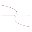
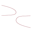
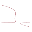
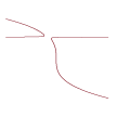
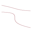
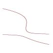
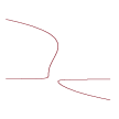
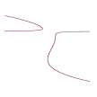
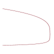
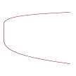
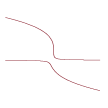
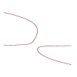
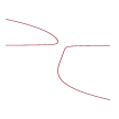
Figure 2: Persistent bifurcation diagrams for parametric singularity $H_{2}$ in (7.2).

Now we consider the parametric germ

$$H_{2}=x^{4}+\lambda x+\alpha_{1}+\alpha_{2}\lambda+\alpha_{3}x^{2},$$ (7.2)

that is a universal unfolding for germ $x^{4}+\lambda x$. Next, $\verb|TransitionSet|(H_{2},[\alpha_{1},\alpha_{2},\alpha_{3}],[x,\lambda])$ gives rise to $\mathscr{B}:=\{(\alpha_{1},\alpha_{2},\alpha_{3})\,|\,\alpha_{2}^{4}+\alpha_{2}^{2}\alpha_{3}+\alpha_{1}=0\}$, $\mathscr{H}:=\{(\alpha_{1},\alpha_{2},\alpha_{3})\,|\,128\alpha_{2}^{2}\alpha_{3}^{3}+3\alpha_{3}^{4}+72\alpha_{1}\alpha_{3}^{2}+432\alpha_{1}^{2}=0\}$, and $\mathscr{D}:=\{(\alpha_{1},\alpha_{2},\alpha_{3})\,|\,\alpha_{3}^{2}-4\alpha_{1}=0,\alpha_{3}\leq 0\}.$ A list of persistent bifurcation diagrams is generated by the command $\verb|PersistentDiagram|(H_{2},[x,\lambda],\verb|plot|,\verb|IntermediateList|)$; Figure 2 is some inequivalent diagrams chosen from this list.

Table 2: Main functions of Singularity associated with the local rings $K[[x,\lambda]],\mathscr{R}$ and $\mathscr{E}$.

Function		Description
StandardBasis		standard basis in either of the rings.
ColonIdeal		computes the colon ideal given in Equation (5.7).
Division		remainder of a germ $g$ divided by a set $G$.
MultMatrix		computes the matrix $\varphi_{u,J}$ in Equations (5.4).
Normalset		finds a basis for complement space of an ideal $I.$

In order to develop Singularity, we have implemented some local tools (suitable in our context) from computational algebraic geometry including division remainders, standard bases, elimination ideals, ideal membership problem and colon ideals for the local rings of fractional (germ) maps, formal power series and smooth maps. These are accordingly implemented in Singularity. We hereby thank Amir Hashemi for his frequent fruitful discussions. We also acknowledge Benyamin M.-Alizadeh’s helps and ideas in the early stages of this project. They were essentially helpful in a fast learning of the concepts from algebraic geometry and their programming. Let

$$G:=\{g_{1}\!:=\sin(\lambda^{7}+x)+\exp(x^{4})-x-1-\lambda^{9},g_{2}\!:=x^{5}-\lambda^{2},g_{3}\!:=\cos(x^{6})-\lambda-1\}$$

and $k$ be a sufficiently large truncation degree. Then using the commands

$$\verb|StandardBasis|(G,[x,\lambda],k,\verb|Fractional|),\verb|StandardBasis|(G,[x,\lambda],k,\verb|Formal|),$$

and $\verb|StandardBasis|(G,[x,\lambda],k,\verb|SmoothGerms|),$ we obtain the Standard basis of $G$ in the rings of fractional maps, formal power series and smooth germs $\mathscr{E}.$ In this example, the standard basis in either of these rings is given by $\{\lambda,x^{3}\}.$ Note that the options $\verb|FormalSeries|$ and $\verb|Fractional|$ in $\verb|StandardBasis|$ use a truncated Taylor series expansion of germs (for non-polynomial and non-fractional germs) and are adapted according to Theorem 4.3. We have already developed some Maple programs for (parametric and orbital) normal form computation, bifurcation analysis and control of singular differential equations [26, 25, 21, 24, 23, 22, 27] and their integration with Singularity shall lead to a toolbox for local bifurcation control and analysis of singularities.

8 An illustrating buckling example

In order to illustrate how Singularity can be used in an application, we borrow a finite element analogue of Euler buckling example from [29, pages 3-10, figures 1.2 and 1.4], i.e., figures 3(a) and 3(b). The associated steady-state solutions (figure 3(a)) follow

$$g(x,\lambda)=\frac{\partial V}{\partial x}(x,\lambda)=x-2\lambda\sin x.$$ (8.1)

The command CheckSingularity$(g,[x,\lambda])$ provides the singular point $(x,\lambda)=(0,\frac{1}{2})$, where $g$ is singular. Verify derives the permissible truncation degree and computational rings, e.g.,

Verify($g,[x,\lambda]$, ’SingularPoint’=’$[0,\frac{1}{2}]$’) leads to

• The following rings are allowed as the means of computations: Ring of smooth germs, Ring of formal power series, Ring of fractional germs, Ring of polynomial germs.

• The truncation degree must be: 4.

• Recommended rings are: Fractional ring, Polynomial ring.

Now the normal form type is derived by Normalform$(g,[x,\lambda],4,$ ’SingularPoint’=’$[0,\frac{1}{2}]$’) as $x^{3}-\lambda x.$ The associated bifurcation diagram can be made available using PersistentDiagram$(x^{3}-\lambda x,[x,\lambda]),$ see figure 3(c).

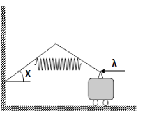
(a)

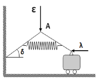
(b)

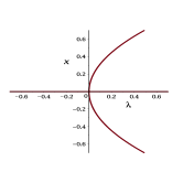
(c)

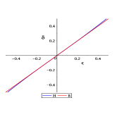
(d)

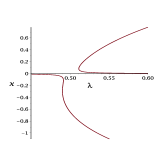
(e)

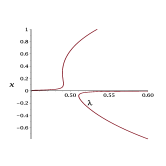
(f)

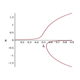
(g)

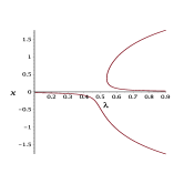
(h)

Figure 3: The buckling models, pitchfork bifurcation diagram, transition set and numerical persistent bifurcation diagrams

Since $g$ is not a universal unfolding, any possible small perturbations of $g$ (such as modeling imperfections) has the potential to dominate the associated dynamics of the problem. Thus, the actual dynamics of the buckling problem does not follow the pitchfork bifurcation diagram 3(c). To treat this caveat, an approach is to determine the universal unfolding of $g$ by the command UniversalUnfolding and accordingly design a universal unfolding model for the buckling experiment via imposing additional parameters into the problem; see [29, 28]. One way to feed the additional unfolding parameters into the problem is to consider them as the controller inputs for a controlled experimental problem. Hence, we may refer to these parameters as the controller inputs. The command UniversalUnfoldingPars can be used in order to find all alternative lists of parameters, where parameters from each list play the role of the universal unfolding parameters; also see [25, section 6] and [19]. This capability is very helpful in a possible alternative modeling refinement of a real life problem. Excluding the extra parameters, the universal unfolding model is obtained. The transition set splits the parameter space into a finite number of connected components. Thereby, the controller inputs should be chosen from the interior part of each connected component (distanced from the component’s boundary). These types of choices for the controller inputs prevent that the qualitative dynamics of the controlled system would be influenced by small perturbations, i.e., the controlled problem is robust against small modeling imperfections.

Using RecognitionProblem($x^{3}-\lambda x,[x,\lambda]$, UniversalUnfolding, Fractional, subs), we obtain

$$\det\left({\begin{array}[]{cccc}0&-1&0&6\\ 0&0&-1&0\\ G_{\alpha_{1}}(0)&G_{\lambda,\alpha_{1}}(0)&G_{x,\alpha_{1}}(0)&G_{x,x,\alpha_{1}}(0)\\ G_{\alpha_{2}}(0)&G_{\lambda,\alpha_{2}}(0)&G_{x,\alpha_{2}}(0)&G_{x,x,\alpha_{2}}(0)\end{array}}\right)\neq 0.$$

We follow [29, Page 7] to consider a small vertical force $\epsilon$ applied on the point $A$ and assuming a zero torque at $x=\delta$, i.e., the spring is at rest when $x:=\delta.$ Hence, the potential function is

$$V(x,\lambda,\epsilon,\delta)=\frac{(x-\delta)^{2}}{2}+2\lambda(\cos x-1)+\epsilon\sin x,$$

with equilibrium equation $G(x,\lambda,\epsilon,\delta):=x-\delta-2\lambda\sin x+\epsilon\cos x=0$.

The command CheckUniversal$(G,[\delta,\epsilon],[x,\lambda],3$, ’SingularPoint’=’$[0,\frac{1}{2}$]’) returns ”yes”, namely $G$ plays the role of universal unfolding for the singular germ $g$.

TransitionSet$(G,[\delta,\epsilon],[x,\lambda]$, ’SingularPoint’=’$[0,\frac{1}{2}]$’) returns

$$\mathscr{B}:=\{(\epsilon,\delta)\,|\,\delta-\epsilon=0\},\quad\mathscr{H}:=\{(\epsilon,\delta)\,|\,\epsilon^{3}-6\delta+6\epsilon=0\},\quad\mathscr{D}:=\emptyset,$$

and $\Sigma:=\mathscr{B}\cup\mathscr{H},$ while TransitionSet$(G,[\delta,\epsilon],[x,\lambda]$, ’SingularPoint’=’$[0,\frac{1}{2}]$’, plot) gives figure 3(d). Finally, the persistent bifurcation diagrams 3(e)-3(h) are derived via

PersistentDiagram($G$, $[\delta,\epsilon]$, $[x,\lambda]$, ’values’=’$[\delta=0.2346,\epsilon=0.2345]$’, ’IntervalPlot’=’$[x=-2..2,\lambda=0.4..0.7]$’) and the same command using the values $(\delta,\epsilon)=(-0.2346,-0.2345),$ $(0.01,-0.01),$ and $(-0.01,0.01),$ respectively.

9 APPENDIX

9.1 Parameter spaces $\mathscr{H}$ and $\mathscr{D}$ for $G_{1}$ given in Equation (7.1)

$\mathscr{H}:=\{(\alpha_{1},\alpha_{2},\alpha_{3},\alpha_{4})\,|\,0=3375\alpha_{2}^{3}\alpha_{3}^{2}\alpha_{4}^{3}+10125\alpha_{1}\alpha_{2}^{2}\alpha_{4}^{4}+16875\alpha_{2}^{3}\alpha_{3}^{4}-675\alpha_{2}^{2}\alpha_{3}^{3}\alpha_{4}^{2}+288\alpha_{2}\alpha_{3}^{2}\alpha_{4}^{4}+67500\alpha_{1}\alpha_{2}^{2}\alpha_{3}^{2}\alpha_{4}-900\alpha_{1}\alpha_{2}\alpha_{3}\alpha_{4}^{3}+864\alpha_{1}\alpha_{4}^{5}+1080\alpha_{2}\alpha_{3}^{4}\alpha_{4}-32\alpha_{3}^{3}\alpha_{4}^{3}+45000\alpha_{1}^{2}\alpha_{2}\alpha_{4}^{2}+13500\alpha_{1}\alpha_{2}\alpha_{3}^{3}+3300\alpha_{1}\alpha_{3}^{2}\alpha_{4}^{2}-108\alpha_{3}^{5}+30000\alpha_{1}^{2}\alpha_{3}\alpha_{4}+50000\alpha_{1}^{3}\}$ and $\mathscr{D}:=\{(\alpha_{1},\alpha_{2},\alpha_{3},\alpha_{4})\,|\,2000\alpha_{2}^{3}\alpha_{4}^{6}+111000\alpha_{2}^{3}\alpha_{3}^{2}\alpha_{4}^{3}-6400\alpha_{2}^{2}\alpha_{3}\alpha_{4}^{5}+64\alpha_{2}\alpha_{4}^{7}+28000\alpha_{1}\alpha_{2}^{2}\alpha_{4}^{4}-16875\alpha_{2}^{3}\alpha_{3}^{4}-43200\alpha_{2}^{2}\alpha_{3}^{3}\alpha_{4}^{2}+5472\alpha_{2}\alpha_{3}^{2}\alpha_{4}^{4}-128\alpha_{3}\alpha_{4}^{6}+45000\alpha_{1}\alpha_{2}^{2}\alpha_{3}^{2}\alpha_{4}-69600\alpha_{1}\alpha_{2}\alpha_{3}\alpha_{4}^{3}+256\alpha_{1}\alpha_{4}^{5}+34020\alpha_{2}\alpha_{3}^{4}\alpha_{4}-1728\alpha_{3}^{3}\alpha_{4}^{3}+130000\alpha_{1}^{2}\alpha_{2}\alpha_{4}^{2}-81000\alpha_{1}\alpha_{2}\alpha_{3}^{3}+43200\alpha_{1}\alpha_{3}^{2}\alpha_{4}^{2}-5832\alpha_{3}^{5}-180000\alpha_{1}^{2}\alpha_{3}\alpha_{4}+200000\alpha_{1}^{3}=0\}.$

References

- [1] D. Armbruster, Bifurcation theory and computer algebra: An initial approach, Lecture Notes in Computer Science 204 (1985) pp. 126–137.
- [2] D. Armbruster and H. Kredel, Constructing universal unfolding using Gröbner basis, J. Symbolic Computation 2 (1986) pp. 383–388.
- [3] T. Becker and V. Weispfenning, Gröbner Bases. A Computational Approach to Commutative Algebra, Graduate Texts in Mathematics 149, 574 pp., Springer Verlag 1993.
- [4] T. Becker, Standard basis in power series rings: uniqueness and superfluous critical pairs, J. Symbolic Computation 15 (1993) pp. 251–265.
- [5] H. Broer, I. Hoveijin, G. Lunter, and G. Vegter, Bifurcations in Hamiltonian systems, Computing Singularities by Gröbner Bases, Springer, Berlin 2003.
- [6] B. Buchberger, An Algorithm for Finding the Basis Elements in the Residue Class Ring Modulo a Zero Dimensional Polynomial Ideal, Mathematical Institute, University of Innsbruck, Austria. PhD Thesis, 1965.
- [7] B. Buchberger, An algorithmic criterion for the solvability of algebraic systems of equations, Aequationes Mathematicae 3 (1970) pp. 374–383.
- [8] B. Buchberger, Groebner-Bases: An algorithmic method in polynomial ideal theory, In: Multidimensional Systems Theory–Progress, Directions and Open Problems in Multidimensional Systems, N.K. Bose (ed.), Chapter 6 (1985) pp. 184–232.
- [9] B. Buchberger, Groebner bases and systems theory, Multidimensional Systems and Signal Processing 12 (3/4) (2001) pp. 223–253.
- [10] C. Chen, O. Golubitsky, F. Lemaire, M. Moreno Maza, and W. Pan, Comprehensive Triangular Decomposition, Lecture Notes in Computer Science 4770 (2007) pp. 73–101.
- [11] R. G. Cowell and F. J. Wright, Computer algebraic tools for applications to catastrophe theory, Europian Conference on Computer Algebra., Lecture Notes in Computer Science, Springer 378 (1987) pp. 71–80.
- [12] D. Cox, J. Little, and D. O’she, Ideals, Varieties, and Algorithms, Springer-Verlag, New York 1991.
- [13] D. Cox, J. Little, and D. O’she, Using Algebraic Geometry, Springer-Verlag, New York 1998.
- [14] W. Decker and G. Pfister, A First Course in Computational Algebraic Geometry, Cambridge University Press, 2013.
- [15] A. Dhooge, W. Govaerts, and Y.A. Kuznetsov, MATCONT: A MATLAB package for numerical bifurcation analysis of ODEs, ACM Transactions on Mathematical Software 29 (2003) pp. 141–164.
- [16] T. Gaffney, Some new results in the classification theory of bifurcation problems, Multiparameter bifurcation theory, Contempary Mathematics 56 (1986) pp. 97–118.
- [17] K. Gatermann and R. Lauterbach, Automatic classification of normal forms, J. Nonlinear Analysis 34 (1988) pp. 157–190.
- [18] K. Gatermann and S. Hosten, Computational algebra for bifurcation theory, J. Symbolic Computation 40 (2005) pp. 1180–1207.
- [19] M. Gazor and M. Kazemi, A user guide for Singularity, ArXiv:1601.00268 (2016).
- [20] M. Gazor and M. Kazemi, Singularity : A Maple library for local zeros of scalar smooth maps, ArXiv:1507.06168v1 July 22, 2015.
- [21] M. Gazor and M. Moazeni, Parametric normal forms for Bogdanov–Takens singularity; the generalized saddle-node case, Discrete and Continuous Dynamical Systems 35 (2015) pp. 205–224.
- [22] M. Gazor, F. Mokhtari, and J.A. Sanders, Normal forms for Hopf–zero singularities with nonconservative nonlinear part, J. Differential Equations 254 (2013) pp. 1571–1581.
- [23] M. Gazor and F. Mokhtari, Volume-preserving normal forms of Hopf–zero singularity, Nonlinearity 26 (2013) pp. 2809–2832.
- [24] M. Gazor and F. Mokhtari, Normal forms of Hopf–zero singularity, Nonlinearity 28 (2015) pp. 311–330.
- [25] M. Gazor and N. Sadri, Bifurcation control and universal unfolding for Hopf–zero singularities with leading solenoidal terms, SIAM J. Applied Dynamical Systems, 15 (2016) pp. 870–903.
- [26] M. Gazor and N. Sadri, Bifurcation controller designs for the generalized cusp plants of Bogdanov-Takens singularity with an application to ship control, ArXiv:1704.07686 (2017).
- [27] M. Gazor and P. Yu, Spectral sequences and parametric normal forms, J. Differential Equations 252 (2012) pp. 1003–1031.
- [28] M. Golubitsky and D. Schaeffer, A theory for imperfect bifurcation via singularity theory, Commun. Pure and Appl. Math. 32 (1979) pp. 1–77.
- [29] M. Golubitsky, I. Stewart, and D. G. Schaeffer, Singularities and Groups in Bifurcation Theory, Volumes 1-2, Springer, New York 1985 and 1988.
- [30] W. Govaerts, Computation of singularities in large nonlinear systems, SIAM J. Numer. Anal. 34 (1997) pp. 867–880.
- [31] W. Govaerts, Numerical Methods for Bifurcations of Dynamical Equilibria, SIAM, 2000.
- [32] G.-M. Greuel and G. Pfister, A Singular Introduction to Commutative Algebra, Springer-Verlag, New York 2007.
- [33] H. Hironaka, Resolution of singularities of an algebraic variety over a field of characteristic zero, Annals Math. 79 (1964) pp. 109–326.
- [34] A. D. Jepson and A. Spence, The numerical solution of nonlinear equations having several parameters I: scalar equations, SIAM J. Number. Anal. 22(4) (1985) pp. 736–759.
- [35] A. D. Jepson and A. Spence, The numerical solution of nonlinear equations having several parameters. Part III: equations with symmetry, SIAM J. Number. Anal. 28(3) (1991) pp. 809–832.
- [36] B. L. Keyfitz, Classification of one state variable bifurcation problems up to codimension seven, Dyn. Stab. Sys. (1986 ) pp. 11–142.
- [37] I. Melbourne, The recognition problem for equivariant singularities, Nonlinearity 1 (1987) pp. 215–240.
- [38] J. Murdock, Normal Forms and Unfoldings for Local Dynamical Systems, Springer-Verlag, New York 2003.
- [39] J. Murdock and T. Murdock, Block Stanley Deompositions II. Greedy Algorithms, Applications and Open Problems, Mathematics Publications, Iowa state University, 104,http://lib.dr.iastate.edu/math_pubs/104, 2017.
- [40] T. Poston and I. Stewart, Catastrophe Theory and Its Applications, Pitman, 1978.
- [41] A. Vutha and M. Golubitsky, Normal forms and unfoldings of singular strategy functions, Dynamic Games and Applications 5 (2014) pp. 180–213.