Magneto-rotational and thermal evolution of young neutron stars

Abstract

After a brief review of population synthesis of close-by cooling neutron stars, I focus on the interpretation of dichotomy of spin periods of near-by coolers. The existence of two well separated groups – short period ($\sim$0.1-0.3 s) radio pulsars and long period ($\sim$3-10 s) radio quiet sources, aka the Magnificent seven, – can not be easily explained in unified models developed recently (Popov et al. 2010, Gullón et al. 2014). I speculate that the most natural solution of the problem can be in bimodal initial magnetic field distribution related to the existence of an additional mechanism of field generation in magnetars.

1 Introduction

Study of neutron stars (NSs) opens unique opportunities to probe regimes where matter is placed under extreme conditions: very high denstity, strong gravity, huge electro-magnetic fields, etc. (see reviews and references in [Potekhin, De Luca, Pons 2014, Weber et al. 2014, Manchester 2015]).

It is possible to confront observational data vs. theoretical explanations and predictions in several ways. Roughly, they can be divided in two categories. In the first, comparison is made using individual sources, in another – population analysis is used, when general properties of a large set of objects are considered together. Typically, the former can give a possibility to go into tiny details. However, some features of the general picture can be missed, and so the population approach is also necessary. The two methods perfectly complement each others.

In this paper I discuss population synthesis of young isolated NSs. Some applications of this method allow us to probe interesting physics of compact objects. In Sect. 2 population synthesis of isolated NSs is very briefly summarized, emphasizing our results on cooling compact objects. Then I discuss joint analysis of several populations of young NSs: radio pulsars, cooling NSs, and magnetars. Sect. 4 provides a description of some new results related to an unexplained feature of the population of near-by cooling isolated NSs. In the last two sections a brief duscussion and conclusions are given.

2 Population synthesis of young NSs

The population synthesis is a powerful technique, and it is widely used in astrophysics, including NS studies ([Popov & Prokhorov 2007]). Historically, first models were devoted to analysis of radio pulsars (see recent studies for example in [Faucher-Giguère & Kaspi 2006, Igoshev & Popov 2014, Gullon et al. 2014] and references therein to earlier papers). Starting from late 90s we developed several population models for different types of isolated compact objects. In this section I briefly summarize our results on near-by cooling NSs.

The population of near-by cooling young isolated NSs was mainly discovered with ROSAT — the German satellite which produced an all-sky survey in soft X-rays (see a review in [Turolla 2009]). There are just about a dozen of such sources. They are either radio pulsars (including Geminga and a geminga-like source), or radio silent (see [Kondratiev et al. 2009] about deep limits on the radio emission of these sources) NSs known as the Magnificent Seven (M7). In the end of 90s the number of these sources was a big puzzle: it was not consistent with general radio pulsar statistics in the Galaxy ([Neuhäuser & Trümper 1999]). Solution was found by Popov et al. (2003).

We demonstrated that the main contribution to the local population of young NSs is done by the Gould Belt. This is a disc-like structure with the size $\sim 0.5$ – 0.7 kpc inclined to the Galactic plane. It consists of OB-associations with ages from few up to 30-50 Myrs. Occasionally, the Sun is situated inside this structure. About 2/3 of young compact objects inside $\sim 0.6$ kpc are genetically related to the Belt.

Later detailed studies of OB-associations distribution in the Belt and behind allowed us to explain the sky distribution of young cooling NSs and make preductions for future searches ([Posselt et al. 2008]).

If we neglect (see below about an alternative approach) an additional heating of compact objects due to magnetic field decay, then all astrophysical parameters of the scenario are relatively well known ([Popov et al. 2005]). This allows us to probe the main physical uncertainty – the rate of NS cooling related to properties of NS interiors. To do it we developed a test of theoretical cooling curves based on population synthesis of near-by NSs, and applied it to two large sets of thermal histories for hadron ([Popov et al. 2006a]) and hybrid ([Popov, Grigorian & Blaschke 2006b]) compact stars.

It was shown that the population synthesis of near-by compact objects can be a powerful additional test for theoretical models of NS cooling. However, in these studies we neglected the additional heating due to the magnetic field decay. For standard radio pulsar fields ($\sim 10^{12}$ G) this assumption is valid, however for magnetars or their descendants – it is not so. Calculations with account for this effect are presented in the next section.

3 Advanced population synthesis of NSs

Usually in population synthesis studies just one subpopulation of a wide class of astronomical objects is modeled. For example, in case of NSs it can be a separate study of normal radio pulsars, or a separate analysis of millisecond pulsars, or (as discussed in the previous section) synthesis of only near-by cooling NSs. In ([Popov et al. 2010]) we made an attempt to model several subpopulations of compact objects in one framework based on the scenario of decaying magnetic field developed by the spanish group leaded by Jose Pons ([Aguilera, Pons & Miralles 2008]).

We used three different codes to model evolution of cooling NSs in the solar proximity, normal radio pulsars, and magnetars. Different distributions have been calculated to compare model predictions with observations. In this study all three approaches have been unified by the same set of initial conditions and basic evolutionary laws. In particular, we used a unique single mode Gaussian distribution for the initial magnetic field of all NSs under study.

Joint analysis of three sets of results allowed us to derive initial distributions for magnetic field and spin period. The best fit was obtained for the initial field distribution with $\langle\log B_{0}/\mathrm{[G]}\rangle\approx 13.25$, $\sigma_{\mathrm{B_{0}}}\approx 0.6$, and for the initial period distribution with $\langle p_{0}\rangle\approx 0.25$ s, $\sigma_{\mathrm{p_{0}}}\approx 0.1$.

For the first time a population synthesis model of three different subpopulations of NSs generated from a unique single-mode initial distribution was shown to be in good correspondence with a large set of observational data. Still, despite significant progress in realizing the research program known as “Grand unification for NSs” ([Kaspi 2010]), there is one feature of the observed population of near-by cooling NSs which we failed to reproduce in our calculations.

4 “One second” problem

In this section we describe an unexplained dip in the spin period distribution of near-by coolers, and discuss some possible solutions of this problem.

4.1 The origin of the problem

Close-by cooling NSs are divided into two main groups: radio pulsars and the M7. They have different spin periods: $\sim 0.1$ – $0.3$ s for pulsars and $\sim 3$ – $10$ s for the M7 (see Fig.1). No sources are observed between $\sim 0.3$ and $\sim$3 s. Oppositely, the calculated distribution is rather smooth. I.e., no sources with spin periods $\sim 1$ s $\pm$ half order of magnitude are observed, but the model predicts them. So, I call it the “one second problem”.

In Fig.1 I present results of calculations for the best model from ([Popov et al. 2010]). In this calculations we were not able to specify the initial period distribution, it has been just assumed that periods are very short. However, for our discussion such simplification is acceptable.

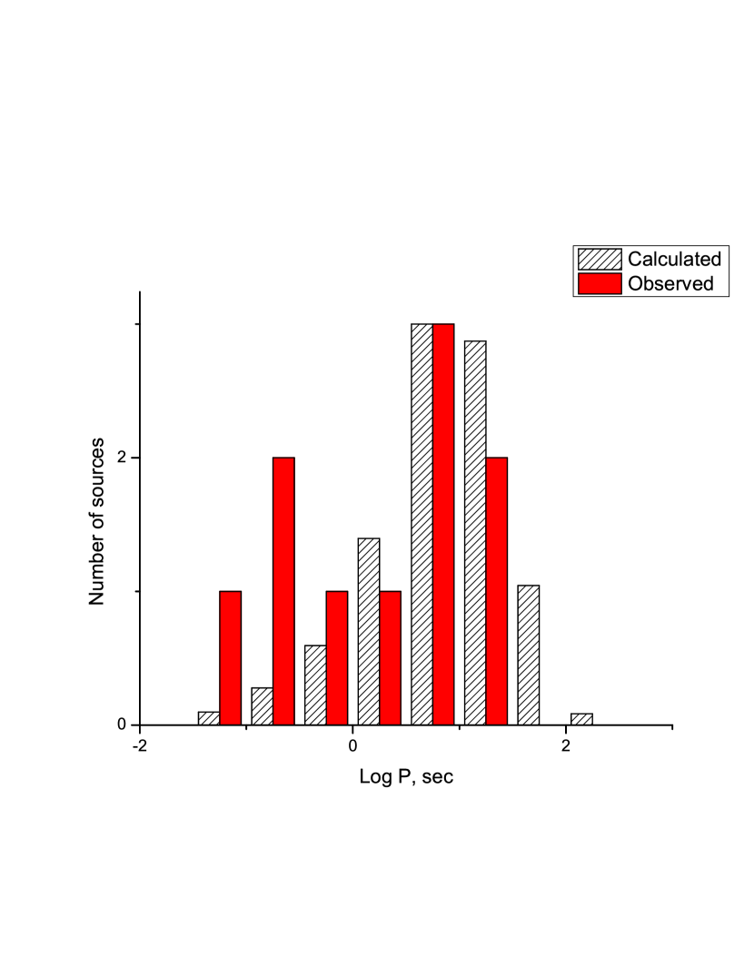
Figure 1: Observed and calculated period distributions for close-by young cooling NSs with ROSAT count rates $>$0.1 cts s^-1. Calculations are done with the model presented in Popov et al. (2010). The observed distribution has a bimodal structure, while the calculated one has just one peak at $p\sim 10$ s. Numbers of sources are equal in two distributions.

The problem can be better illustrated with the $p$ – $\dot{p}$ plot. In Fig. 2 I present this diagram for our results. A number of the observed sources in each bin is shown with digits. The scale for the amount of modeled sources in not normalized because here the idea is just to demonstrate that even by shape these two distributions are very different. The synthetic distribution is single-peaked with a maximum close to the position of the M7. I.e., in the theoretical model we have a lack of cooling NSs with standard fields $\sim 10^{12}$ G (similar to normal pulsars).

Figure 2: The $p$ – $\dot{p}$ distribution for close-by young cooling NSs with ROSAT count rates $>0.1$ cts s^-1. Grey scale represents results of our calculations with the evolutionary model described in Popov et al. (2010). Total amount of calculated sources was not normalized. Numbers correspond to the data on real sources (four radio pulsar-like sources, and five of the M7, for which $p$ and $\dot{p}$ are well-measured.

This deficit is also visible in Fig.3 where I show the magnetic field distribution for NSs which contribute to the population with relatively large ROSAT fluxes ($\ga 0.1$ cts s ^-1, see Fig. 4). There are very few NSs with fields $\sim 10^{12}$ G among bright sources in the synthetic model. On one hand, this discrepancy can be due to low statistics in the observational data. But most probably, there is a more physical reason behind it. For example, the synthesis can predict smaller number of short spin period sources if temperatures of standard field NSs can be underestimated in theoretical cooling curves.

Figure 3: Magnetic field distribution for modeled sources presented in Figs.1 and 2. Only bright sources with ROSAT count rates $>0.1$ cts s^-1 contribute to the statistics. Number of sources is not normalized.

4.2 New cooling curves

Vigano et al. (2013) produced a different set of cooling curves, in which temperature of objects with $B\la 3\times 10^{12}$ G is higher than in the pervious variant (used in [Popov et al. 2010]). The results of population synthesis modeling with new tracks is shown in Figs.4-6.

I used the same initial magnetic field distribution, and the same assumptions about the period evolution as in ([Popov et al. 2010]). The Log $N$ – Log $S$ distribution is not influenced significantly, and the model nicely follows the data, Fig. 4. But the spin period distribution for bright sources (Fig.6) and $p$ –$\dot{p}$ (Fig.5) plot are notably modified.

Figure 4: The Log $N$ – Log $S$ distribution for close-by NSs calculated with new evolutionary tracks by Vigano et al. (2013). Solid line corresponds to the results of calculations. The horizintal axis is for ROSAT counts per second. Symbols represent the observed sources. Filled symbols correspond to addition to the distribution of one of the M7 sources, opaque — to a radio pulsar. Poissonian errors are shown. The BSC limit corresponds to the ROSAT Bright Source catalogue (Voges et al. 1999).

With the new cooling curves it is possible to increase the number of NSs with standard fields among X-ray bright population. Still, spin period and $p$ –$\dot{p}$ distributions are again single-peaked, and so we do not see two separate populations of sources.

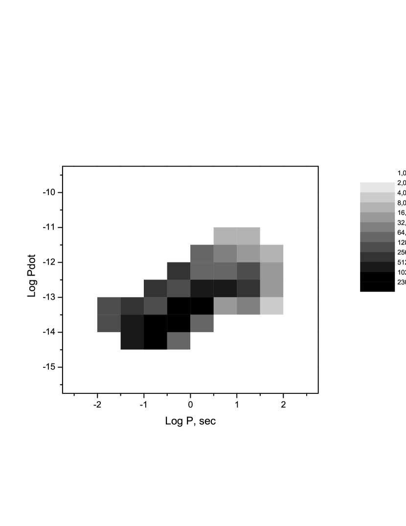
Figure 5: The $p$ – $\dot{p}$ distribution for the new evolutionary tracks by Vigano et al. (2013). Numbers of sources are not normalized.

While potentially it can be possible to fit a cooling history in such a way that one obtains two separate populations, or at least can fit the data taking into account low statistics of known sources, I do not think that this is a real solution to the problem.

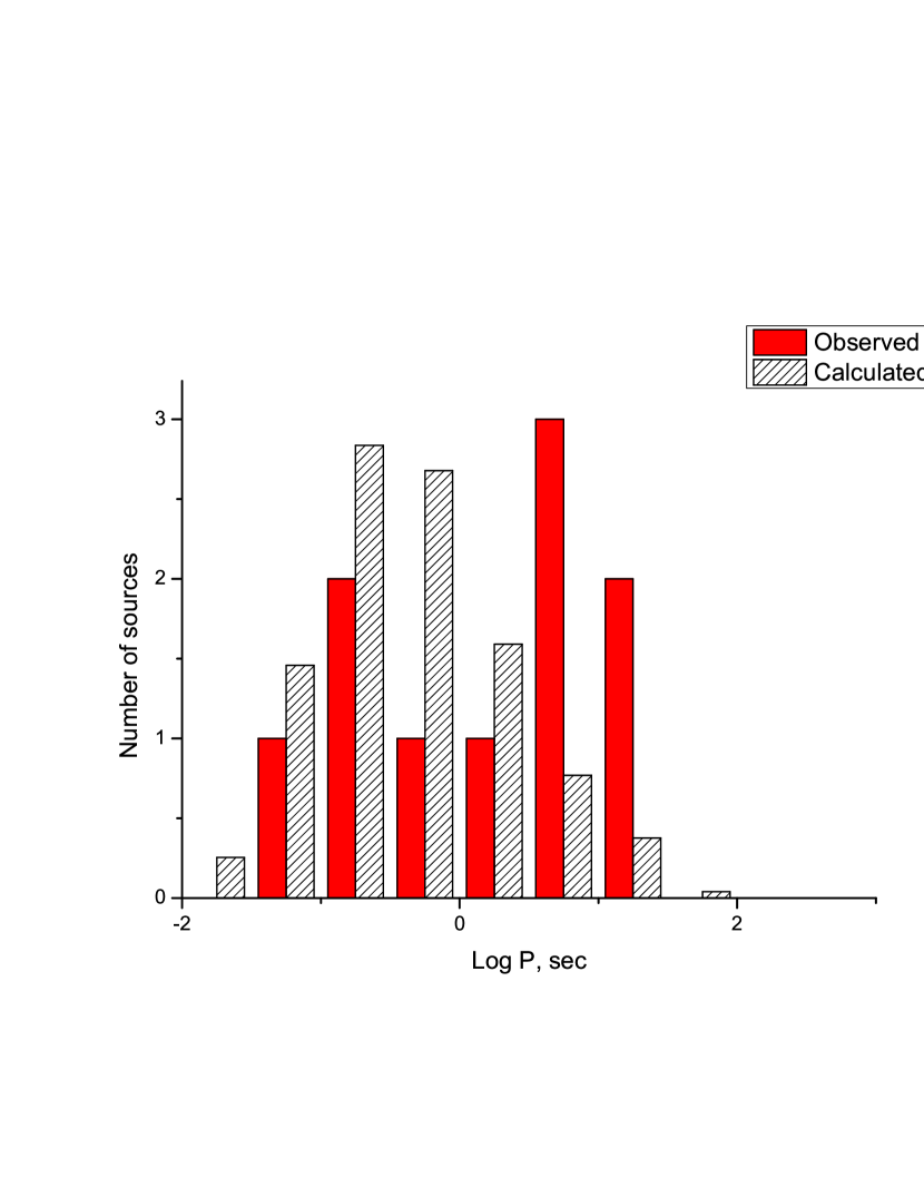
Figure 6: Observed and calculated period distributions. Calculations are done with the new evolutionary tracks by Vigano et al. (2013). Total numbers of sources are equal in two distributions.

4.3 No field decay

One solution of the “one second” problem can be related to a bimodal initial magnetic field distribution. Such a distribution is favoured if there is an additional mechanism for enhancing magnetic field of magnetars and other highly magnetized NSs.

I briefly illustrate this using the cooling curves by St. Petersburg group ([Shternin et al. 2011]). In this model the thermal evolution of NSs is not related to their magnetic field evolution (and so the spin period evolution is not linked with the thermal evolution). In the simplest case we can assume constant fields.

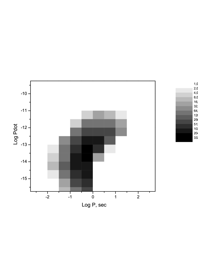
Figure 7: The $p$ – $\dot{p}$ distribution for constant magnetic fields and cooling according to Shternin et al. (2011). Magnetic field distribution is Gaussian with $\sigma_{\mathrm{B}}=0.55$ and $\langle\log B_{0}/\mathrm{[G]}\rangle=12.65$.

At first I show $p$ – $\dot{p}$ distribution for the case when the initial parameters are distributed according to ([Faucher-Giguère & Kaspi 2006]). The initial magnetic field and the initial spin periods both have Gaussian distributions (for the field in log scale): $\langle\log B_{0}/\mathrm{[G]}\rangle\approx 12.65$, $\sigma_{\mathrm{B_{0}}}\approx 0.55$ and $\langle p_{0}/\mathrm{[s]}\rangle\approx 0.3$, $\sigma_{\mathrm{p_{0}}}\approx 0.15$.

The Log $N$ – Log $S$ distribution can be obtained in correspondence with observations for realistic NS mass spectrum (now it is crucial, as there is no additional heating due to field decay, and cooling is determine by internal NS structure and processes). As expected, the $p$ – $\dot{p}$ distribution is single-peaked.

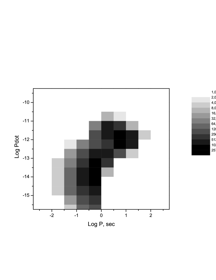
Figure 8: The $p$ – $\dot{p}$ distribution for constant magnetic fields and cooling according to Shternin et al. (2011). Magnetic field distribution consists of two Gaussians. The low-field one provides 60% of NSs and has $\sigma_{\mathrm{B}}=0.5$ and $\langle\log B_{0}/\mathrm{[G]}\rangle=12.5$. The high-field part has $\sigma_{\mathrm{B}}=0.15$ and $\langle\log B_{0}/\mathrm{[G]}\rangle=14$.

Just for an illustration, I also produce a plot for a double-peaked field distribution, Fig 8. Note, that here no additional heating is added. In this artificial distribution the low-field part contributes 60% of NSs and has $\langle\log B_{0}/\mathrm{[G]}\rangle\approx 12.5$, $\sigma_{\mathrm{B_{0}}}\approx 0.5$. The high-field distribution has $\langle\log B_{0}/\mathrm{[G]}\rangle\approx 14$, $\sigma_{\mathrm{B_{0}}}\approx 0.15$. As before only sources with ROSAT count rate $\geq 0.1$ cts s^-1 contribute to the statistics.

As we can see, obviously it is possible to fit the data playing with the initial magnetic field distribution. The same can be done in the model with decaying field.

5 Discussion

In this note it is demonstrated that the bimodal period distribution of near-by cooling NSs cannot be explained if their initial field distribution is single-mode unless some unrealistic fitting assumptions are made. The population synthesis is not able to probe the situation deeper because models of thermal and magneto-rotational evolution are not very certain in several aspects. Only progess in understanding the NS physics might help to solve this problem.

The explanation of the dip around $\sim 1$ s in the period distribution by a bimodal field distribution can be justified by proposals of a separate mechanism of field enhancement in magnetars ([Thompson & Duncan 1993]), and by the possibility of separate evolutionary channels which produce them ([Popov & Prokhorov 2006]). Otherwise, we have to assume that a single smooth initial field distribution in the range from $\la 10^{11}$ G up to $\sim 10^{15}$ G is due to a unique mechanism, which is doubtful.

“Grand unification of NSs” is not complete until central compact objects (CCOs) are included in the general picture. Now the most promising approach is related to the idea of re-emerging magnetic field ([Ho 2011, Vigano & Pons 2012], Bernal, Page & Lee 2013). In this scenario magnetic field of a NS is submerged in an episode of fall-back accretion. Such objects can appear as CCOs – low-field thermal emitters without radio pulsar activity. Then on time scale $\sim 10^{4}$ yrs this field diffuses out. Objects which passed this stage potentially can contribute to the local population of coolers, as their fraction is estimated to be high – up to 30%. How the existence of such objects influences the spin period distribution of close-by cooling NSs is not known.

Finally, discussing near-by cooling NSs we are still dealing with low statistics. Since ROSAT time no new near-by candidates have been reported (see [Agüeros et al. 2011] for a recent attempt to identify more cooling NSs). Only more distant candidates are discussed, and their nature is still somehow uncertain ([Pires et al. 2012]). I hope very much that in near future more close-by cooling NSs can be discovered, in the first place thanks to eROSITA on-board Spectrum-RG. The prediction is that new discoveries will confirm the dip around one second in the spin period distribution of near-by coolers.

6 Conclusions

Here I presented the results on population synthesis modeling of period and $p$ – $\dot{p}$ distributions for young cooling NSs in the solar vicinity. It is shown that both calculated distributions are single mode for a single mode initial magnetic field distribution. This does not fit observational data. The number of observed objects is not large, however as they not only form two subpopulations in both distributions, but also the observational properties of sources in each mode are different (radio pulsars vs. M7), I take this dichotomy as a serious fact.

The problem can be solved either via fine tunning of thermal and magneto-rotational evolution of NSs, or via assuming bimodal initial field distribution. The second possibility seems to be more realistic. In this case the M7 becomes more closely related to magnetars, i.e. their initial fields might be enhanced similarly to magnetar fields.