Speeding up MCMC by delayed acceptance and data subsampling

Abstract.

The complexity of the Metropolis-Hastings (MH) algorithm arises from the requirement of a likelihood evaluation for the full data set in each iteration. Payne and Mallick, (2015) propose to speed up the algorithm by a delayed acceptance approach where the acceptance decision proceeds in two stages. In the first stage, an estimate of the likelihood based on a random subsample determines if it is likely that the draw will be accepted and, if so, the second stage uses the full data likelihood to decide upon final acceptance. Evaluating the full data likelihood is thus avoided for draws that are unlikely to be accepted. We propose a more precise likelihood estimator which incorporates auxiliary information about the full data likelihood while only operating on a sparse set of the data. We prove that the resulting delayed acceptance MH is more efficient compared to that of Payne and Mallick, (2015). The caveat of this approach is that the full data set needs to be evaluated in the second stage. We therefore propose to substitute this evaluation by an estimate and construct a state-dependent approximation thereof to use in the first stage. This results in an algorithm that (i) can use a smaller subsample $m$ by leveraging on recent advances in Pseudo-Marginal MH (PMMH) and (ii) is provably within $O(m^{-2})$ of the true posterior.

Keywords: Bayesian inference, Markov chain Monte Carlo, Delayed acceptance MCMC, Large data, Survey sampling

1. Introduction

Markov Chain Monte Carlo (MCMC) methods have been the workhorse for sampling from nonstandard posterior distributions in Bayesian statistics for nearly three decades. Recently, with increasingly more complex models and/or larger data sets, there has been a surge of interest in improving the $O(n)$ complexity emerging from the necessity of a complete data scan in each iteration of the algorithm.

There are a number of approaches proposed in the literature to speed up MCMC. Some authors divide the data into different partitions and carry out MCMC for the partitions in a parallel and distributed manner. The draws from each partition’s subposterior are subsequently combined to obtain an approximation of the full posterior distribution. This line of work includes Scott et al., (2013); Neiswanger et al., (2013); Wang and Dunson, (2013); Minsker et al., (2014); Nemeth and Sherlock, (2016), among others. Other authors use a subsample of the data in each MCMC iteration to speed up the algorithm, see e.g. Korattikara et al., (2014), Bardenet et al., (2014), Maclaurin and Adams, (2014), Maire et al., (2015), Bardenet et al., (2015) and Quiroz et al. (2016, 2017). Finally, delayed acceptance MCMC has been used to speed up computations (Banterle et al.,, 2014; Payne and Mallick,, 2015). The main idea in delayed acceptance is to avoid computations if there is an indication that the proposed draw will ultimately be rejected. Payne and Mallick, (2015) consider a two stage delayed acceptance MCMC that uses a random subsample of the data in the first stage to estimate the likelihood function at the proposed draw. If this estimate suggests that the proposed draw is likely to be rejected, the algorithm does not proceed to the second stage that evaluates the true likelihood (using all data). Banterle et al., (2014) divide the acceptance ratio in the standard Metropolis-Hastings (MH) (Metropolis et al.,, 1953; Hastings,, 1970) into several stages, which are sequentially performed until a first rejection is detected implying a final rejection of the proposed draw. Clearly, both delayed acceptance approaches save computations for proposals that are unlikely to be accepted, but on the other hand require all stages to be computed for those likely to be accepted. The latter corresponds to at least the same computational cost for one iteration as the standard MH.

This paper extends the delayed acceptance algorithms of Payne and Mallick, (2015) in the following directions. First, we replace the likelihood estimator of the first stage by an efficient estimator that employs control variates to significantly reduce the variance. We show that this modification results in an algorithm which is more effective in promoting good proposals to the second stage. Since this algorithm computes the true likelihood (as does MH) in the second stage whenever a draw is up for a final accept/reject decision, we refer to it as Delayed Acceptance (standard) MH (DA-MH). Second, we propose a delayed acceptance algorithm that overcomes the caveat of a full data likelihood evaluation in the second stage by replacing it with an estimate. This second stage estimate is initially developed in the approximate subsampling Pseudo-Marginal MH (PMMH) framework in Quiroz et al., (2016). Thus, our second contribution is to speed up their algorithm by combining with delayed acceptance and we document large speedups for our so called Delayed Acceptance PMMH (DA-PMMH) algorithm compared to MH. Payne and Mallick, (2015) instead propose to circumvent the full data evaluation by combining their delayed acceptance sampler with the consensus Monte Carlo in Scott et al., (2013), which currently lacks any control of the error produced in the approximate posterior. In contrast, we can make use of results in Quiroz et al., (2016) to control the approximation error and also ensure that it is $O(m^{-2})$, where $m$ is the subsample size used for estimating the likelihood.

While the delayed acceptance MH has the disadvantage of using all data whenever a proposed draw proceeds to the second stage, we believe that the successful implementation provided here is essential if exact simulation is of importance. By exact simulation we mean that the Markov chain produced by the subsampling algorithm has the same invariant distribution as that of a Markov chain produced by an algorithm that uses all the data. Exact simulation using subsets of the data has proven to be extremely challenging. Pseudo-marginal MCMC (Beaumont,, 2003; Andrieu and Roberts,, 2009) provides a framework for conducting Markov chain simulation by only using an estimate (in this setting estimated from a subsample of the data) of the likelihood. Remarkably, although the true likelihood is never evaluated, the simulation is exact provided that the likelihood estimate is unbiased and almost surely positive. One route to exact simulation by data subsampling suggested by Bardenet et al., (2015) is to compute a sequence of unbiased estimators of the log-likelihood, apply the technique in Rhee and Glynn, (2015) to debias the resulting likelihood estimator and subsequently use it within a pseudo-marginal MCMC. Bardenet et al., (2015) note that, as proved by Jacob and Thiery, (2015), a lower bound on the log-likelihood estimators is needed to ensure positiveness. This typically requires computations using the full data set, naturally defeating the purpose of subsampling. Quiroz et al., (2017) instead suggests to compute a soft lower bound which is defined to be a lower bound with a high probability. Since the estimate can occasionally be negative, the pseudo-marginal in Quiroz et al., (2017) instead targets an absolute measure following Lyne et al., (2015), who show that the draws can be corrected with an importance sampling type of step to estimate expectations of posterior functions exactly. We note that although this certainly is exact inference of the expectation (it is not biased) the algorithm does not provide exact simulation as defined above. Maclaurin and Adams, (2014) propose Firefly Monte Carlo, which introduces an auxiliary variable for each observation, which determines if it is included when evaluating the likelihood. The distribution of these binary variables is such that when they are integrated out, the marginal posterior is the same as the one targeted by MH, thus providing exact simulation. Typically a small fraction of observations are included, hence speeding up the execution time significantly compared to MH. However, the augmentation scheme severely affects the mixing of the Firefly algorithm and it has been demonstrated to perform poorly compared to MH and other subsampling approaches (Bardenet et al.,, 2015; Quiroz et al.,, 2016, 2017). We conclude that delayed acceptance, out of the discussed methods, seems to be the only feasible route to obtain exact simulation via data subsampling. We demonstrate that our implementation is crucial to obtain an algorithm that can improve on MH.

This paper is organized as follows. Section 2 presents the efficient likelihood estimator. Sections 3 and 4 outline the delayed acceptance MH and PMMH methodologies in the context of subsampling. Section 5 applies the method to a micro-economic data set containing nearly 5 million observations. Section 6 concludes and Appendix A proves Theorem 1.

2. Likelihood estimators with subsets of data

2.1. Structure of the likelihood

Let $\theta$ be the parameter in a model with density $p(y_{k}|\theta,x_{k})$, where $y_{k}$ is a potentially multivariate response vector and $x_{k}$ is a vector of covariates for the $k$th observation. Let $l_{k}(\theta)=\log p(y_{k}|\theta,x_{k})$ denote the $k$th observation’s log-density, $k=1,\dots,n$. Given conditionally independent observations, the likelihood function can be written

(2.1) $$p(y|\theta)=\exp\left[l(\theta)\right],$$

where $l(\theta)=\sum_{k=\text{1}}^{n}l_{k}(\theta)$ is the log-likelihood function. To estimate $p(y|\theta)$, we first estimate $l(\theta)$ based on a sample of size $m$ from the population $\left\{l_{1}(\theta),\dots,l_{n}(\theta)\right\}$ and subsequently use (2.1). The first step corresponds to the classical survey sampling problem of estimating a population total: see Särndal et al., (2003) for an introduction to survey sampling. Note that (2.1) is more general than identically independently distributed (iid) observations, although we require that the log-likelihood can be written as a sum of terms, where each term depends on a unique piece of data information. One example is models with a random effect for each subject, with possibly multiple individual observations per subject (longitudinal data). In this case, a single term in the log-likelihood sum corresponds to the log joint density for a subject, and we therefore sample subjects (rather than individual observations) when estimating (2.1).

2.2. Data subsampling

A main distinction of sampling schemes is whether the sample is obtained with or without replacement. It is clear that sampling with replacement gives a higher variance for any function of the sample: including the same element more than once does not provide any further information about finite population characteristics. However, it results in sample elements that are independent which facilitates the derivation of Theorem 1 for the delayed acceptance MH. It also allows us to apply the theory and methodology in Quiroz et al., (2016) for the delayed acceptance PMMH in Section 4. It should be noted that the two sampling schemes are approximately the same when $m\ll n$.

Let $u=(u_{1},\dots u_{m})$ be a vector of indices obtained by sampling $m$ indices with replacement from $\{1,\dots,n\}$ and let $\left\{l_{u_{1}}(\theta),\dots,l_{u_{m}}(\theta)\right\}$ be the sample. We will consider Simple Random Sampling (SRS) which means that

$$\Pr(u_{i}=k)=\frac{1}{n}\text{ for }k=1,\dots,n,\text{ and for all }i=1,\dots,m.$$

Payne and Mallick, (2015) use SRS (but without replacement) to form an unbiased estimate of the log-likehood. However, the elements $l_{k}(\theta)$ (for a fixed $\theta$) vary substantially across the population and estimating the total $\sum_{k=1}^{n}l_{k}(\theta)$ with SRS is well known to be very inefficient under such a scenario. Instead $\Pr(u_{i}=k)$ should be (approximately) proportional to a size measure for $l_{k}(\theta)$. Quiroz et al., (2016) argue that this so called Proportional-to-Size sampling is in many cases unlikely to be successful as knowledge of a size measure (which also depends on $\theta$) for all $k$ can often defeat the purpose of subsampling. They instead propose to use SRS but incorporate control variates in the estimator for variance reduction which we now turn to.

2.3. Efficient log-likelihood estimators

The idea in Quiroz et al., (2016) is to homogenize the population $\left\{l_{1}(\theta),\dots,l_{n}(\theta)\right\}$: if the resulting elements are roughly of the same size then SRS is expected to be efficient. Let $q_{k}(\theta)$ denote an approximation of $l_{k}(\theta)$ and decompose

$$l(\theta) = \sum_{k=1}^{n}q_{k}(\theta)+\sum_{k=1}^{n}\left[l_{k}(\theta)-q_{k}(\theta)\right]$$

$$= q(\theta)+d(\theta),$$

where

$$q(\theta)=\sum_{k=1}^{n}q_{k}(\theta),\quad d(\theta)=\sum_{k=1}^{n}d_{k}(\theta),\quad\text{and}\quad d_{k}(\theta)=l_{k}(\theta)-q_{k}(\theta).$$

We emphasize that all quantities depend on $\theta$ which, from now on, is sometimes suppressed for a compact notation.

Define the random variables $\eta_{i}=nd_{u_{i}}$ and $d_{u_{i}}=l_{u_{i}}-q_{u_{i}}$ with $\mathrm{E}[\eta_{i}]=d$ and

$$\sigma_{\eta}^{2}=\mathrm{V}[\eta_{i}]=n^{2}\mathrm{V}[d_{u_{i}}]=n\sum_{k=1}^{n}(d_{k}-\bar{d})^{2},\quad\text{with }\bar{d}=\sum_{k=1}^{n}d_{k}.$$

The difference estimator estimates $d$ in (2.3) with the Hansen-Hurwitz estimator (Hansen and Hurwitz,, 1943),

$$\hat{d}_{m}=\frac{1}{m}\sum_{i=1}^{m}\eta_{i},\quad\text{with }\mathrm{E}[\hat{d}_{m}]=d\quad\text{and}\quad\mathrm{V}[\hat{d}_{m}]=\frac{\sigma_{\eta}^{2}}{m}.$$

We can obtain an unbiased estimate $\hat{\sigma}_{\eta}^{2}=n^{2}\mathrm{\hat{V}}[d_{u_{i}}]$, where $\hat{\mathrm{V}}[d_{u_{i}}]$ is the usual unbiased sample variance estimator (of the population $\{d_{1},\dots d_{n}\}$). The estimator of the log-likelihood is thus

(2.3) $$\hat{l}_{m}=\sum_{k=1}^{n}q_{k}(\theta)+\hat{d}_{m},\quad\text{with }\mathrm{E}[\hat{l}_{m}]=l\quad\text{and}\quad\sigma^{2}=\mathrm{V}[\hat{l}_{m}]=\frac{\sigma_{\eta}^{2}}{m}.$$

It also follows that $\hat{\sigma}_{m}^{2}=\hat{\sigma}_{\eta}^{2}/m$ is an unbiased estimator of $\sigma^{2}$.

Quiroz et al., (2016) reason that observations close in data space $(x_{k},y_{k})$ should, for a fixed $\theta$, have similar $l_{k}(\theta)$ values. They cluster the data space into $K$ clusters and approximate, within each cluster, $l_{k}(\theta)$ by a second order Taylor series expansion $q_{k}(\theta)$ around the centroid of the cluster. This allows computing $q$ using $K$ evaluations (instead of $n$), see Quiroz et al., (2016) for details. Bardenet et al., (2015) propose similar control variates, but instead expand with respect to $\theta$ around a reference value $\theta^{\star}$. While it can be shown that $q$ can be computed using a single evaluation, the approximation can be inaccurate when $\theta$ is far from $\theta^{\star}$ giving a large $\sigma^{2}$.

We note that the log-likelihood estimate in Payne and Mallick, (2015) (if with replacement sampling is used) is a special case of (2.3), namely when $q_{k}=0$ for all $k$. We will see that this results in a poor performance of the delayed acceptance algorithm and that control variates are crucial for a successful implementation.

2.4. Approximately bias-corrected likelihood estimator

It is clear that an unbiased log-likelihood estimator becomes biased for the likelihood when transformed to the ordinary scale by the exponential function. Since by the Central Limit Theorem (CLT)

$$\sqrt{m}\left(\hat{l}_{m}(\theta)-l(\theta)\right)\rightarrow\mathcal{N}(0,\sigma_{\eta}^{2})\quad\text{as}\quad m\rightarrow\infty,$$

Quiroz et al., (2016) (see also Ceperley and Dewing, 1999; Nicholls et al., 2012) approximately bias corrects the likelihood estimate

(2.4) $$\hat{p}_{m}(y|\theta,u)=\exp\left(\hat{l}_{m}(\theta)-\hat{\sigma}_{\eta}^{2}(\theta)/2m\right).$$

Equation (2.4) is unbiased if $\sigma_{\eta}^{2}$ is used in place of $\hat{\sigma}_{\eta}^{2}$ (and normality holds for $\hat{l}_{m}$). In practice we need to use $\hat{\sigma}_{\eta}^{2}$ (to not use all data) and Quiroz et al., (2016) show that (2.4) is asymptotically unbiased, with the bias decreasing as $O(m^{-2})$. For the rest of the paper we refer to (2.4) as a “bias-corrected” estimator, where the quotation marks highlight that the correction is not exact.

3. Delayed acceptance MH with subsets of data

3.1. The algorithm

Payne and Mallick, (2015) propose a subsampling delayed acceptance MH following Christen and Fox, (2005). The aim in delayed acceptance is to simulate a Markov chain $\{\theta^{(j)}\}_{j=1}^{N}$ which admits the posterior

$$\pi(\theta)=\frac{p(y|\theta)p(\theta)}{p(y)},\text{ where }p(y)=\int p(y|\theta)p(\theta)d\theta\text{ and }p(\theta)\text{ denotes the prior,}$$

as invariant distribution. Moreover, the likelihood $p(y|\theta)$ should only be evaluated if there is a good chance of accepting the proposed $\theta$.

The algorithm in Payne and Mallick, (2015) proceeds as follows. Let $\theta_{c}=\theta^{(j)}$ denote the current state of the Markov chain. In the first stage, propose $\theta^{\prime}\sim q_{1}(\theta|\theta_{c})$ and compute

(3.1) $$\alpha_{1}(\theta_{c}\rightarrow\theta^{\prime}) = \min\left\{1,\frac{\hat{p}_{m}(y|\theta^{\prime},u)p(\theta^{\prime})/q_{1}(\theta^{\prime}|\theta_{c})}{\hat{p}_{m}(y|\theta_{c},u)p(\theta_{c})/q_{1}(\theta_{c}|\theta^{\prime})}\right\},$$

where $\hat{p}_{m}(y|\theta,u)$ is the estimator in Section 2.4 without control variates for $\hat{l}_{m}$ (but not “bias-corrected”, see below). Now, propose

$$\theta_{p}=\begin{cases}\theta^{\prime}&\quad\text{w.p.}\quad\alpha_{1}(\theta_{c},\theta^{\prime})\\ \theta_{c}&\quad\text{w.p.}\quad 1-\alpha_{1}(\theta_{c},\theta^{\prime}),\end{cases}$$

and move the chain to the next state $\theta^{(j+1)}=\theta_{p}$ with probability

(3.2) $$\alpha_{2}(\theta_{c}\rightarrow\theta_{p}) = \min\left\{1,\frac{p(y|\theta_{p})p(\theta_{p})/q_{2}(\theta_{p}|\theta_{c})}{p(y|\theta_{c})p(\theta_{c})/q_{2}(\theta_{c}|\theta_{p})}\right\},$$

where

$$q_{2}(\theta_{p}|\theta_{c}) = \alpha_{1}(\theta_{c}\rightarrow\theta_{p})q_{1}(\theta_{p}|\theta_{c})+r(\theta_{c})\delta_{\theta_{c}}(\theta_{p}),\quad r(\theta_{c})=1-\int\alpha_{1}(\theta_{c}\rightarrow\theta_{p})q_{1}(\theta_{p}|\theta_{c})d\theta_{p},$$

and $\delta$ is the Dirac delta function. If rejected we set $\theta^{(j+1)}=\theta_{c}$.

Note that $\alpha_{2}$ in (3.2) is equivalent to the acceptance probability of a standard MH with a proposal density $q_{2}(\theta_{p}|\theta_{c})$ that is a mixture of two proposal densities: the first proposes to move from $\theta_{c}$ to $\theta_{p}$ (from the “slab” $q_{1}$) and the second proposes to stay at $\theta_{c}$ (from the “spike”). The mixture weight for the “slab” is $\alpha_{1}$ in (3.1) (with $\theta^{\prime}=\theta_{p}$): if the likelihood estimate is higher at $\theta^{\prime}$ compared to that of $\theta_{c}$ (after correcting with $q_{1}$) we propose $\theta^{\prime}=\theta_{p}$ with probability 1. Conversely, if it is lower, we propose to move but with a probability smaller than 1 which decreases the less likely we think that $\theta^{\prime}$ will be accepted as indicated by the estimated likelihood. The estimator $\hat{p}_{m}(y|\theta^{\prime},u)$ used by Payne and Mallick, (2015) does not depend on the current state of the Markov chain and hence the mixture weights in $q_{2}$ are state-independent. Convergence to the invariant distribution therefore follows from standard MH theory. The same applies when the estimator uses the control variates in Quiroz et al., (2016), or in Bardenet et al., (2015) but only for a fixed $\theta^{\star}$. Bardenet et al., (2015) suggest setting $\theta^{\star}=\theta_{c}$ every now and then to prevent that the control variates can be poor if the chain is far from $\theta^{\star}$: the resulting approximation is clearly state-dependent and standard MH theory does not apply. Instead, convergence to the invariant $\pi(\theta)$ is proved in Christen and Fox, (2005) and the delayed algorithm is exactly as above but with

$$\hat{p}_{m}(y|\cdot,u)=\hat{p}_{m}^{(\theta_{c})}(y|\cdot,u),\quad\text{emphasizing that it depends on the current state }\theta_{c}.$$

The state-dependent algorithm is a key ingredient when developing the delayed acceptance block PMMH in Section 4.

As noted above, Payne and Mallick, (2015) do not “bias correct” the likelihood estimate as they point out that the algorithm will have the correct invariant distribution anyway. We remark that without control variates it is not a good idea to apply the correction as the variance of $\hat{\sigma}_{m}^{2}$ is huge which adversely affects $\hat{p}_{m}(y|\cdot,u)$. An efficient estimate of $\hat{\sigma}_{m}^{2}$, however, would certainly improve $\hat{p}_{m}(y|\cdot,u)$. While the control variates allow us to estimate $\hat{\sigma}_{m}^{2}$ accurately, we will not implement the “bias-correction” when comparing to Payne and Mallick, (2015) in order to make the comparison fair.

It is beneficial to also update $u$ in order to avoid the risk of having a subset of observations for which the approximation is poor. This is especially important for the estimator in Payne and Mallick, (2015), as not using control variates can result in the particular subset having highly heterogeneous elements, which is detrimental for SRS. We note that updating $u$ is still a valid MH because (i) $u$ is not a state of the Markov chain and (ii) the distribution $p(u)=1/n^{m}$ (SRS) does not depend on $\theta$. Thus, the transition kernel of an algorithm that updates $u$ is a state-independent mixture of transition kernels, where each of the kernels satisfies detailed balance either by standard MH (or Christen and Fox, (2005) if the approximation depends on $\theta_{c}$). Since the weights $1/n^{m}$ do not depend on $\theta$, it follows that the mixture also satisfies detailed balance, and thus has $\pi(\theta)$ as invariant distribution. It is unnecessary to update $u$ in every iteration, instead one can update $u$ randomly to save the overhead cost of indexing the data matrix when obtaining the subset of observations.

We remark that delayed acceptance (sometimes with names as early rejection or surrogate transition), although without data subsampling, has been considered earlier in the literature. References include Fox and Nicholls, (1997); Liu, (2008); Cui et al., (2011); Smith, (2011); Solonen et al., (2012); Golightly et al., (2015); Sherlock et al., 2015a . Each stage in Banterle et al., (2014) (see Section 1) uses a partition of the data and can thus be considered as delayed acceptance with data subsampling. The advantage of our algorithm is that, because it only has two stages and the second stage evaluates the full data likelihood, we can instead estimate this likelihood in order to never do the evaluation for the full data set, see Section 4.

3.2. Efficiency of delayed acceptance MH when subsampling the data

When considering efficiency of MCMC algorithms with additional computational costs (e.g. estimating the target), there are two types of fundamentally different efficiencies that interplay. The first is the statistical efficiency, which we will measure by the asymptotic (as the number of MCMC iterates go to infinity) variance of an estimate based on output from the Markov chain. Consider two MCMC algorithms $\mathcal{A}_{1}$ and $\mathcal{A}_{2}$ with the same invariant distribution. Then $\mathcal{A}_{1}$ is statistically more (less) efficient than $\mathcal{A}_{2}$ if it has a lower (higher) asymptotic variance. The second is the computational efficiency, which solely concerns “execution time” to produce a given number of iterates. The measures of statistical and computational efficiency (and a combination of them) used in this article are presented later in this section.

Sherlock et al., 2015b (in a non-subsampling context) study the statistical efficiency for delayed acceptance random walk Metropolis and, moreover, an efficiency that also takes into account the computational efficiency for the case where the target is estimated (DA-PMMH in Section 4).

Christen and Fox, (2005) note that, because the transition kernels of both the MH and delayed acceptance MH are derived from the same proposal $q_{1}$, and in addition $\alpha_{2}\leq 1$, the delayed acceptance MH will be less statistically efficient than MH. The intuition is that under these conditions the chain clearly exhibits a more “sticky” behavior and an estimate based on these samples will have a larger asymptotic variance under DA-MH than MH. Notice that the closer $\alpha_{2}$ is to $1$, the more statistically efficient the delayed acceptance algorithm is, and when $\alpha_{2}=1$ it is equivalent to the standard MH which gives the upper bound of the possible statistical efficiency achieved by a DA-MH.

Result 1 in Payne and Mallick, (2015) gives the alternative formulation (for state-independent approximations)

(3.3) $$\alpha_{2}(\theta_{c}\rightarrow\theta_{p}) = \min\left\{1,\frac{\hat{p}_{m}(y|\theta_{c},u)/p(y|\theta_{c})}{\hat{p}_{m}(y|\theta_{p},u)/p(y|\theta_{p})}\right\}.$$

Let $l_{k}(\theta_{c},\theta_{p})=l_{k}(\theta_{c})-l_{k}(\theta_{p})$ and denote by $\hat{l}_{m}(\theta_{c},\theta_{p})$ the estimate of $l(\theta_{c},\theta_{p})=\sum_{k=1}^{n}l_{k}(\theta_{c},\theta_{p})$. Similarly to (2.3),

(3.4) $$\hat{l}_{m}(\theta_{c},\theta_{p}) = q(\theta_{c},\theta_{p})+\frac{1}{m}\sum_{i=1}^{m}\zeta_{i},\quad\text{with }q(\theta_{c},\theta_{p})=\sum_{k=1}^{n}q_{k}(\theta_{c},\theta_{p}),$$

where $q_{k}(\theta_{c},\theta_{p})=q_{k}(\theta_{c})-q_{k}(\theta_{p})$ and the $\zeta_{i}$’s are iid with

$$\Pr\left(\zeta_{i}=nD_{k}(\theta_{c},\theta_{p})\right)=\frac{1}{n},\text{ with }D_{k}=\left(l_{k}(\theta_{c},\theta_{p})-q_{k}(\theta_{c},\theta_{p})\right)\quad\text{for }i=1,\dots m.$$

We can also show that

(3.5) $$\mathrm{E}[\hat{l}_{m}(\theta_{c},\theta_{p})]=l(\theta_{c},\theta_{p})\text{ and }V[\hat{l}_{m}(\theta_{c},\theta_{p})]=\frac{\sigma_{\zeta}^{2}}{m}\text{ with }\sigma_{\zeta}^{2}=n\sum_{k=1}^{n}\left(D_{k}(\theta_{c},\theta_{p})-\bar{D}_{F}(\theta_{c},\theta_{p})\right)^{2},$$

where $\bar{D}_{F}$ is the mean over the full population. When not “bias-corrected”, the ratio appearing in (3.3) becomes

(3.6) $$R_{m}=\exp\left(\hat{l}_{m}(\theta_{c},\theta_{p})-l(\theta_{c},\theta_{p})\right).$$

We now propose a theorem that relates $\mathrm{E}\left[\alpha_{2}(\theta_{c}\rightarrow\theta_{p})\right]$ to the variance $\sigma_{R}^{2}=\mathrm{V}[\hat{l}_{m}(\theta_{c},\theta_{p})]$ under the assumption that $\hat{l}_{m}(\theta_{c},\theta_{p})\sim\mathcal{N}(l(\theta_{c},\theta_{p}),\sigma_{R}^{2})$ (equivalently $R_{m}\sim\log\mathcal{N}(0,\sigma_{R}^{2})$ in (3.6)). In turn, $\alpha_{2}$ relates to the statistical efficiency as discussed above. The assumption of normality is justified by a standard CLT for $\hat{l}_{m}(\theta_{c},\theta_{p})$ since the $\zeta_{i}$’s are iid.

Theorem 1.

Suppose that we run a DA-MH with a state-independent approximation

$$\hat{l}_{m}(\theta_{c},\theta_{p})\sim\mathcal{N}\left(l(\theta_{c},\theta_{p}),\sigma_{R}^{2}\right),\quad\text{where }\sigma_{R}^{2}(\theta_{c},\theta_{p})=\mathrm{V}[\log(R_{m})],$$

which has a second stage acceptance probability

$$\alpha_{2}(\theta_{c}\rightarrow\theta_{p})=\min\left(1,R_{m}\right),\quad R_{m}=\exp\left(\hat{l}_{m}(\theta_{c},\theta_{p})-l(\theta_{c},\theta_{p})\right).$$

Then

$$\mathrm{E}[\alpha_{2}(\theta_{c}\rightarrow\theta_{p})] = \exp\left(\sigma_{R}^{2}(\theta_{c},\theta_{p})/2\right)\left(1-\Phi\left(\sigma_{R}(\theta_{c},\theta_{p})\right)\right)+0.5.$$

In particular, $\mathrm{E}[\alpha_{2}(\theta_{c}\rightarrow\theta_{p})]$ is a decreasing function of $\sigma_{R}$.

Proof.

See Appendix A. ∎

Remark.

It is possible to state and prove a similar theorem using a “bias-corrected” likelihood estimator, which in log-scale is $\hat{l}_{m}(\theta_{c},\theta_{p})-\hat{\sigma}{}_{R}^{2}(\theta_{c},\theta_{p})/2$. This is omitted as our application in Example 1 in Section 5 does not use a “bias-corrected” likelihood estimator in order to conduct a fair comparison to Payne and Mallick, (2015).

Theorem 1 says that if the variance of the log of the ratio $R_{m}$ in (3.6) is lower, then the algorithm has a higher $\alpha_{2}$ on average. Moreover, it shows that $\alpha_{2}$ deteriorates quickly with $\sigma_{R}$, which illustrates the importance of achieving a small $\sigma_{R}$.

Although the delayed acceptance MH is always less statistically efficient than MH it can of course still be more generally efficient in terms of balancing computational and statistical efficiency. Clearly, a necessary condition to achieve a more general efficient DA-MH algorithm than the corresponding MH requires that its computing time is faster, i.e. it must be computationally more efficient. When comparing DA-MH algorithms with the same computing time (by for example having the same subsample size) then Theorem 1 shows that a smaller variance of the log-ratio results in a more general efficient algorithm.

To also compare algorithms of different computing times we now define a measure for the general efficiency discussed above. In the rest of the paper, whenever we claim that algorithms are more or less efficient to each other it is based on this measure. The statistical (in)efficiency part is measured by the Inefficiency Factor (IF), which quantifies the amount by which the variance of $(1/N)\sum_{j=1}^{N}\theta^{(j)}$ is inflated when $\theta^{(j)}$ is obtained by Markov chain simulation compared to that of iid simulation. It is given by

(3.7) $$\mathrm{IF} = 1+2\sum_{l=1}^{\infty}\rho_{l},$$

where $\rho_{l}$ is the auto-correlation at the $l$th lag of the chain, and can be computed with the coda package in R (Plummer et al.,, 2006). To include computational efficiency in the measure we use Effective Draws (ED) per computing unit

(3.8) $$\mathrm{ED} = \frac{N}{\mathrm{IF}\times t},$$

where $N$ is the number of MCMC iterations and $t$ is the computing time. The measure of interest is the effective draws per computing time of a delayed acceptance algorithm $\mathcal{A}$ relative to that of MH, i.e.

(3.9) $$\mathrm{RED} = \frac{\mathrm{ED}^{\mathcal{A}}}{\mathrm{ED}^{\mathrm{MH}}}.$$

4. Delayed acceptance PMMH with subsets of data

4.1. PMMH for data subsampling

Quiroz et al., (2016) propose a pseudo-marginal approach to subsampling based on the “bias-corrected” likelihood estimator in (2.4). In the next subsection this estimate replaces the true likelihood, thereby avoiding the evaluation of the full data set. To allow for a smaller subsample size without adversely affecting the mixing of the chain Quiroz et al., (2016) develop a correlated pseudo-marginal approach based on Deligiannidis et al., (2016). Tran et al., (2016) (see also Quiroz et al.,, 2016) use an alternative approach to correlated pseudo-marginal which we use for our Delayed Acceptance Block PMMH (DA-BPMMH) in Section 4.3. Although not considered here, it is straightforward to instead correlate the subsamples as in Deligiannidis et al., (2016).

Pseudo-marginal by data subsampling targets the following posterior on an augmented space $(\theta,u)$,

(4.1) $$\tilde{\pi}_{m}(\theta,u)=\hat{p}_{m}(y|\theta,u)p(u)p(\theta)/p_{m}(y),\text{ with }p_{m}(y)=\int p_{m}(y|\theta)p(\theta)d\theta.$$

The algorithm is similar to MH except that $\theta$ and $u$ are proposed and accepted (or rejected) jointly, with probability

(4.2) $$\alpha_{\mathrm{PMMH}} = \min\left\{1,\frac{\hat{p}_{m}(y|\theta_{p},u_{p})p(\theta_{p})/q(\theta_{p}|\theta_{c})}{\hat{p}_{m}(y|\theta_{c},u_{c})p(\theta_{c})/q(\theta_{c}|\theta_{p})}\right\},$$

where the subscripts denote the current and proposed values of $\theta$ and $u$. Quiroz et al., (2016) show that the algorithm converges to a slightly perturbed target (only approximately unbiased likelihood estimator) $\pi_{m}(\theta)$ and prove that

$$\frac{\left|\pi_{m}(\theta)-\pi(\theta)\right|}{\pi(\theta)}\leq O(m^{-2}).$$

Moreover, if $h(\theta)$ is a function that is absolutely integrable with respect to $\pi(\theta)$, then $\mathrm{E}_{\pi_{m}}\left[h(\theta)\right]$ is also within $O(m^{-2})$ of its true value.

The variance of $\hat{l}_{m}$ is crucial for the general efficiency of the algorithm: $\sigma^{2}$ in the approximate interval $[1,3.3]$ is optimal (Pitt et al.,, 2012; Doucet et al.,, 2015; Sherlock et al., 2015c, ). The correlated pseudo-marginal approach induces a high positive correlation between the estimates in (4.2) by correlating $u_{c}$ and $u_{p}$. This allows the use of a less precise estimator without getting stuck: the errors in the numerator and denominator tend to cancel. As a consequence, $\sigma^{2}$ can be larger than above, hence speeding up the algorithm by taking a smaller subsample. We follow Tran et al., (2016) and divide $u$ (defined in Section 2.2) into $G$ blocks,

$$u=(u_{(1)},\dots,u_{(G)})\quad\text{with }\frac{m}{G}\text{ observations within each block,}$$

and update a single block (randomly) in each iteration. Setting $G$ large induces a high positive correlation $\rho$ between $\hat{l}_{m}(\theta_{c})$ and $\hat{l}_{m}(\theta_{p})$: Tran et al., (2016) show that $\rho=1-1/G$ under certain assumptions. We set $G=100$ for the state-dependent algorithm in our application.

4.2. State-independent algorithm: DA-PMMH

Delayed acceptance PMMH uses an estimate of the target in the second stage of the algorithm. Such algorithms have recently been considered by Sherlock et al., 2015b ; Sherlock et al., 2015a and Golightly et al., (2015). We propose a state-independent data subsampling DA-PMMH (uncorrelated PMMH) and a state-dependent (block PMMH, where the correlation between the subsamples follows Tran et al.,, 2016) extension DA-Block (correlated) PMMH (DA-BPMMH) in the next subsection.

The estimated “bias-corrected” likelihood in (2.4) is approximated in a first stage screening by $\hat{s}$ which is discussed in Section 4.4. Similarly to the algorithm in Section 3.1, we desire to only evaluate the (estimated) target (on the augmented space) if the proposed state is likely to be accepted. Let $\left(\theta_{c},u_{c}\right)=\left(\theta^{(j)},u^{(j)}\right)$ denote the current state of the augmented Markov chain. In the first stage, propose $\theta^{\prime}\sim q_{1}(\theta|\theta_{c})$ and $u^{\prime}\sim p(u)$ and evaluate

(4.3) $$\alpha_{1}^{\mathrm{PMMH}}\left\{\left(\theta_{c},u_{c}\right)\rightarrow\left(\theta^{\prime},u^{\prime}\right)\right\} = \min\left\{1,\frac{\hat{s}(\theta^{\prime},u^{\prime})p(\theta^{\prime})/q_{1}(\theta^{\prime}|\theta_{c})}{\hat{s}(\theta_{c},u_{c})p(\theta_{c})/q_{1}(\theta_{c}|\theta^{\prime})}\right\},$$

where $\hat{s}(\theta,u)$ is the approximation of $\hat{p}_{m}(y|\theta,u)$ (2.4). Propose

$$\left(\theta_{p},u_{p}\right)=\begin{cases}\left(\theta^{\prime},u^{\prime}\right)&\quad\text{w.p.}\quad\alpha_{1}^{\mathrm{PMMH}}\left\{\left(\theta_{c},u_{c}\right)\rightarrow\left(\theta^{\prime},u^{\prime}\right)\right\}\\ \left(\theta_{c},u_{c}\right)&\quad\text{w.p.}\quad 1-\alpha_{1}^{\mathrm{PMMH}}\left\{\left(\theta_{c},u_{c}\right)\rightarrow\left(\theta^{\prime},u^{\prime}\right)\right\},\end{cases}$$

and move to $\left(\theta^{(j+1)},u^{(j+1)}\right)=\left(\theta_{p},u_{p}\right)$ with probability

(4.4) $$\alpha_{2}^{\mathrm{PMMH}}\left\{\left(\theta_{c},u_{c}\right)\rightarrow\left(\theta_{p},u_{p}\right)\right\} = \min\left\{1,\frac{\hat{p}_{m}(y|\theta_{p},u_{p})p(\theta_{p})/q_{2}(\theta_{p}|\theta_{c})}{\hat{p}_{m}(y|\theta_{c},u_{c})p(\theta_{c})/q_{2}(\theta_{c}|\theta_{p})}\right\},$$

where

$$q_{2}(\theta_{p}|\theta_{c}) = \alpha_{1}^{\mathrm{PMMH}}q_{1}(\theta_{p}|\theta_{c})+r(\theta_{c})\delta_{\theta_{c}}(\theta_{p}),\quad r(\theta_{c})=1-\int\alpha_{1}^{\mathrm{PMMH}}q_{1}(\theta_{p}|\theta_{c})d\theta_{p},$$

and $\delta$ is the Dirac delta function. If rejected we set $\left(\theta^{(j+1)},u^{(j+1)}\right)=\left(\theta_{c},u_{c}\right)$. Similarly to the argument for the DA-MH, we recognize $\alpha_{2}^{\mathrm{PMMH}}$ as the acceptance probability for a pseudo-marginal algorithm. Since the approximation is state-independent ($\hat{s}(\theta,u)$ independent of the current state implies state-independent mixture weights for $q_{2}$), convergence follows from being a pseudo-marginal algorithm (Andrieu and Roberts,, 2009). However, as the estimate is biased the target is perturbed (Quiroz et al.,, 2016) but within $O(m^{-2})$ as discussed in Section 4.1.

4.3. State-dependent algorithm: DA-BPMMH

As $u$ is part of the state in a pseudo-marginal algorithm, obtaining a state-dependent approximation is easily achieved by correlating $u$: we sample $u_{p}\sim p(u|u_{c})$ thus $\hat{s}(\theta,u)=\hat{s}_{\theta_{c},u_{c}}(\theta,u)$. This is the state-dependent (on the augmented space) setup in Christen and Fox, (2005) and it follows that the invariant distribution is $\tilde{\pi}_{m}(\theta,u)$ in (4.1). This is the invariant distribution in the algorithm in Quiroz et al., (2016), which we already mentioned has a marginal $\pi_{m}(\theta)$ within $O(m^{-2})$ of $\pi(\theta)$. We note that this state-dependent approximation is very convenient because it automatically allows us to have a higher variance on $\hat{l}_{m}$ because of the block PMMH mechanism (see Section 4.1).

4.4. An approximation of the estimated likelihood

Our approximation is inspired by adaptive delayed acceptance ideas in Cui et al., (2011) and Sherlock et al., 2015a . However, our approach is not strictly adaptive as we only learn about the proposal for a fixed training period of $N_{\mathrm{train}}$ iterations, which are discarded from the final draws.

The idea is to use a sparser set of the data to construct control variates $q_{k}^{(1)}(\theta)$ in the first stage. During the training period we learn about the discrepancy between $q^{(1)}(\theta)=\sum_{k=1}^{n}q_{k}^{(1)}(\theta)$ and $q(\theta)$ of the second stage (obtained with a denser set), i.e.

(4.5) $$\underbrace{q(\theta)-q^{(1)}(\theta)}_{=e(\theta)}=f(\theta)+\epsilon,\quad\epsilon\text{ is the noise (assumed independent of $\theta$)}.$$

Learning about $f$ is a standard regression problem: the collection of proposed $\theta$’s during the fixed training period are the inputs and the discrepancies are the training data.

The trivial decomposition

$$\hat{l}_{m}(\theta) = \sum_{k=1}^{n}q_{k}(\theta)+\hat{d}_{m}(\theta)-\hat{\sigma}_{m}^{2}/2$$

$$= \sum_{k=1}^{n}q_{k}^{(1)}(\theta)+\left(\sum_{k=1}^{n}q_{k}(\theta)-\sum_{k=1}^{n}q_{k}^{(1)}(\theta)\right)+\hat{d}_{m}(\theta)-\hat{\sigma}_{m}^{2}/2$$

suggests the first stage approximation

$$\hat{s}(\theta,u)=\sum_{k=1}^{n}q_{k}^{(1)}(\theta)+\hat{e}(\theta)+\hat{d}_{m}(\theta)-\hat{\sigma}_{m}^{2}/2,$$

where $\hat{e}(\theta)$ is the prediction of the discrepancy at $\theta$. Note that computing the true discrepancy requires the denser set to be evaluated, whereas the prediction is very fast. For example, in linear (or non-linear by basis functions) regression the parameters of $f(\theta)$ are estimated once after the training data has been collected. Prediction of $e(\theta)$ for a new “data-observation” $\theta$ is then a simple dot product computation, which is typically much faster than evaluating $q(\theta)$. Note that if the $u$’s are correlated then $\hat{s}(\theta,u)$ also depends on the current state, i.e. $\hat{s}_{\theta_{c},u_{c}}(\theta,u)$.

In Section 5 we implement both a linear regression and (noise free) Gaussian process to learn $f$ in (4.5), but any regression technique can be used.

5. Application

5.1. Data and model

We model the probability of bankruptcy conditional on a set of covariates using a data set of $534,717$ Swedish firms for the time period 1991-2008. We have in total $n=4,748,089$ firm-year observations. The variables included are: earnings before interest and taxes, total liabilities, cash and liquid assets, tangible assets, logarithm of deflated total sales and logarithm of firm age in years. We also include the macroeconomic variables GDP-growth rate (yearly) and the interest rate set by the Swedish central bank. See Giordani et al., (2014) for a detailed description of the data set.

We consider the logistic regression model

$$p(y_{k}|x_{k},\beta) = \left(\frac{1}{1+\exp(x_{k}^{T}\beta)}\right)^{y_{k}}\left(\frac{1}{1+\exp(-x_{k}^{T}\beta)}\right)^{1-y_{k}},$$

where $x_{k}$ includes the variables above plus an intercept term. We set $p(\beta)\sim N(0,10I)$ for simplicity. Since the bankruptcy observations $(y_{k}=1)$ are sparse in the data, we follow Payne and Mallick, (2015) and estimate the likelihood only for the $y_{k}=0$ observations. That is, we decompose

$$l(\beta) = \sum_{\{k;y_{k}=1\}}l_{k}(\beta)+\sum_{\{k;y_{k}=0\}}l_{k}(\beta),$$

and evaluate the first term whereas a random sample is only taken to estimate the second term. The second term clearly follows the structure presented in Section 2.1.

5.2. Performance evaluation measures

The quantity of interest is the effective draws as defined in (3.8). We now outline how to compute $t$ as CPU time and present an alternative measure independent of the implementation that is based number of evaluations. We first outline a robust measure of the CPU time.

The delayed acceptance algorithms we implement have two stages, where the first stage is filtering out draws unlikely to be accepted. One can view MH as an algorithm that does not filter any proposed draws at all: any draw is subject to an accept/reject decision based on the second stage likelihood. To make total CPU time comparisons fair between a Delayed Acceptance (DA) MH and its corresponding MH, we compute the total time for the latter (MH) by the median time the former (DA) spends in the second stage and multiply by the number of MCMC iterations $N$:

$$\mathrm{CPU}_{\mathrm{MH}}=N\times\text{median time $\mathrm{DA}$ stage 2}.$$

The median is used to avoid extreme values that can arise due to external disturbances (CPU time should be independent of $\theta$ here). For the delayed acceptance algorithm the CPU time is

$$\mathrm{CPU}_{\mathrm{DA}}=N\times\text{median time $\mathrm{DA}$ stage 1}\text{ }+\mathrm{FullEval\times\text{median time $\mathrm{DA}$ stage 2},}$$

where $\mathrm{FullEval}$ is the number of second stage evaluations the delayed acceptance performs.

The (total) number of evaluations measure is straightforward for MH ($N\times n$), DA-MH without control variates ($N\times m+\mathrm{FullEval}\times n$) and with ($N\times(K+m)+\mathrm{FullEval}\times n$), and PMMH/BPMMH ($N\times(K+m)$). For the delayed versions of PMMH/BPMMH we similarly add the different evaluations, but note that it will be different for the pre- and post- training period. Moreover, there is a one time cost of learning $f(\theta)$ and also a (post-training) cost of predicting $e(\theta)$. We translate these to number of evaluations as follows. First, for learning $f(\theta)$ we measure the CPU time it takes to fit it with the training data. We compare this time to the average CPU time for the iterations during the training period. We do so because we know the measure of the latter in terms of number of evaluations: $K^{(1)}+K+m$, where $K^{(1)}$ and $K$ are, respectively, the number of centroids in the sparser and denser set of data. Therefore, if learning $f(\theta)$ is say $T$ times slower in CPU time, then this translates to $T\cdot(K^{(1)}+K+m)$ number of evaluations. Finally, the number of evaluations for predicting a single $e(\theta)$ depends on the model for $f(\theta)$. For linear regression the prediction is a dot product which we assign the same cost as computing a single log-likelihood contribution (which is typically a function of a dot product). For a Gaussian process, the prediction requires evaluating the kernel for $N_{\mathrm{train}}$ observations and we let that define the number of evaluations for a single prediction.

5.3. Implementation details

We consider the following two examples. Example 1 estimates the model with DA-MH implemented with our efficient control variates and compares it to the implementation in Payne and Mallick, (2015). Example 2 estimates the model with DA-BPMMH and compare to the block PMMH algorithm in Quiroz et al., (2016). To make comparisons fair for Example 1 we use without replacement sampling (as in Payne and Mallick,, 2015). This sampling scheme is typically used together with the Horvitz-Thompson estimator (Horvitz and Thompson,, 1952): see Särndal et al., (2003) on how to modify the formulas in Section 2.3 for without replacement sampling.

Two main implementations of the difference estimator are considered. The first computes $q_{k}$ with the second order term evaluated at $\beta$, which we call dynamic. The second, which we call static, fixes the second order term at the optimum $\beta^{\star}$. The dynamic approach clearly provides a better approximation but is more expensive to compute. For both the dynamic and static approaches we compare four different sparse representations of the data for computing $q$ in (2.3), each with a different number of clusters. The clusters are obtained using Algorithm 1 in Quiroz et al., (2016) on the observations for which $y=0$ ($4,706,523$ observations). We note that, as more clusters are used to represent the data, the approximation of the likelihood is more accurate, although it is more expensive to compute.

We consider a Random walk MH proposal for $\beta$ where we learn the proposal scale during the first $N_{\mathrm{train}}=5,000$ (and also train $f(\theta)$) iterations in order to reach an acceptance probability of $\approx 0.23$ for MH (Roberts et al.,, 1997) and $\approx 0.10$ for BPMMH. For the delayed acceptance algorithms we have the same targets but for $\alpha_{1}$, i.e. the first stage acceptance probability. We discard the training samples and also a subsequent burn-in period of $10$% of the remaining samples ($20,000$) when doing inference. However, the computing costs (CPU and number of evaluations) include all $N$ iterations.

Finally, the delayed acceptance algorithms are implemented with an update of $u$ with probability $0.01$.

5.4. Example 1: DA-MH

Tables 1 and 2 summarize the results, respectively, for the difference estimator with control variates (DE) and the estimator in Payne and Mallick, (2015) (PM). It is evident that the difference estimator has a larger second stage acceptance probability $\alpha_{2}$ (for a given sample size), which is a consequence of Theorem 1 because it has a lower $\sigma_{R}^{2}=V[\log(R_{m})].$ Figure 5.1 confirms that the normality assumptions, for the smallest value of $m$ and $K$ (the worst case scenario), are adequate for both methods. We also note from Table 2 that for some sample sizes Payne and Mallick, (2015) performs more poorly than the standard Metropolis-Hastings algorithm. One possible explanation is that the applications in Payne and Mallick, (2015) have a small number of continuous covariates (one in the first application and three in the second) and the rest are binary. It is clear that the continuous covariate case results in more variation among the log-likelihood contributions which is detrimental for SRS. In this application we have eight continuous covariates which explains why SRS without covariates performs poorly for small sampling fractions. As an example, for a subsample of $0.1\%$ of the data, not a single effective sample was obtained.

Table 1. Delayed acceptance MH with control variates. The table shows some quantities for the static and dynamic implementation with different sparse representations of the data represented by $K$, which is the number of clusters (expressed as % of $n$). For each approximation different sample sizes ($0.1,1,5$ in % of $n$) are considered. The quantities are the mean $\mathrm{RED}_{1}$ and $\mathrm{RED}_{2}$ in (3.9) measured with respect to computing time and average number of evaluations, respectively. Furthermore, $\bar{\sigma}_{R}$ is the mean (over MCMC iterations) standard deviation of $\log(R_{m})$. Finally, $\alpha_{1}$ and $\alpha_{2}$ are the acceptance probabilities in (3.1) and (3.3) (expressed in %), where the latter is computed conditional on acceptance in the first stage. The corresponding MH algorithm has an acceptance rate of $\approx$$23$%.

		Static										Dynamic
		$\mathrm{RED}_{1}$		$\mathrm{RED}_{2}$		$\bar{\sigma}_{R}$		$\alpha_{1}$		$\alpha_{2}$		$\mathrm{RED}_{1}$		$\mathrm{RED}_{2}$		$\bar{\sigma}_{R}$		$\alpha_{1}$		$\alpha_{2}$
	$K=0.03$
	0.1	0.93		0.95		5.90		22		14		2.35		2.56		1.48		23		57
	1	2.43		2.65		1.40		22		59		2.23		3.47		0.45		22		85
	5	2.09		2.78		0.57		24		82		0.73		3.27		0.19		24		93
	$K=0.21$
	0.1	1.51		1.52		3.87		21		24		2.87		2.84		0.83		25		74
	1	2.81		3.02		0.99		22		69		3.03		3.91		0.27		22		91
	5	2.05		2.71		0.39		26		88		0.78		3.17		0.11		25		96
	$K=0.71$
	0.1	2.24		2.20		2.10		21		46		3.03		3.49		0.41		23		86
	1	3.53		3.30		0.60		22		81		1.97		3.70		0.13		23		96
	5	2.22		3.09		0.26		22		92		0.70		3.28		0.06		24		98
	$K=3.68$
	0.1	2.64		2.75		0.82		21		74		1.28		3.63		0.13		21		96
	1	3.71		3.19		0.25		23		92		1.15		3.57		0.04		21		99
	5	3.60		2.93		0.11		23		96		0.60		2.95		0.02		24		99

Table 2. Delayed acceptance MH without control variates (Payne and Mallick,, 2015). The table shows some quantities for different sample sizes ($0.1,1,5,50,80$, in % of $n$) to estimate the likelihood. The quantities are the mean $\mathrm{RED}_{1}$ and $\mathrm{RED}_{2}$ in (3.9) measured with respect to computing time and number of evaluations, respectively. Furthermore, $\bar{\sigma}_{R}$ is the mean (over MCMC iterations) standard deviation of $\log(R_{m})$. Finally, $\alpha_{1}$ and $\alpha_{2}$ are the acceptance probabilities in (3.1) and (3.3) (expressed in %), where the latter is computed conditional on acceptance in the first stage. The corresponding MH algorithm has an acceptance rate of $\approx$$23$%.

		$\mathrm{RED}_{1}$		$\mathrm{RED}_{2}$		$\bar{\sigma}_{R}$		$\alpha_{1}$		$\alpha_{2}$
	0.1	0.00		0.00		101.94		21		0
	1	0.36		0.37		13.81		18		3
	5	1.39		1.45		3.52		22		29
	50	1.13		1.33		0.63		24		80
	80	0.91		1.08		0.31		24		90

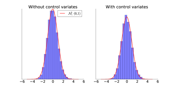
Figure 5.1. Addressing the normality assumption in Theorem 1. The figure shows a histogram of (standardized) $\hat{l}_{m,n}(\theta_{c},\theta_{p})$ in (3.4) ($10,000$ Monte Carlo replicates) without control variates (left, Payne and Mallick,, 2015) and with control variates (right). The red solid line is the density function of a standard normal variable. The validation is for the smallest value of $m$ ($0.1$% of $n$) for both cases and for the smallest value of $K$ (less accurate, $0.03$% of $n$) for the control variates. The values of the parameters are $\theta_{c}=\theta^{\star}$, where $\theta^{\star}$ is the mode, and $\theta_{p}$ is sampled from the proposal distribution. We have verified the assumption for several values of $\theta_{c}$ and $\theta_{p}$ (not shown here).

5.5. Example 2: DA-BPMMH

Our second example explores how the state-dependent delayed acceptance BPMMH improves the BPMMH proposed in Quiroz et al., (2016). The results are presented in Table 3. Quiroz et al., (2016) in turn show that they outperform other subsampling approaches and, in particular, that many of these approaches perform more poorly than the standard MH (see also Bardenet et al.,, 2015) in terms of efficiency and/or can give a very poor approximation of the posterior. Here we find that the delayed acceptance BPMMH is 30 times more efficient than MH, which is a huge improvement considering the aforementioned facts. Moreover, we find that the approximate posterior produced is very close to the true posterior (simulated by MH), as illustrated in Figure 5.2.

Table 3. Delayed acceptance block PMMH. The table shows some quantities for Block PMMH (BPMMH, Quiroz et al.,, 2016) and delayed acceptance BPMMH. The latter is implemented with a Gaussian Process (GP) and Linear Regression (LR) for learning $f(\theta)$ to predict $e(\theta)$ in (4.5). The block PMMH use a sample size of $0.5$% which corresponds to $\sigma^{2}\approx 10$. The approximations used by BPMMH for computing the likelihood estimate is based on $K=3.68$ (expressed as % of $n$) number of clusters. The delayed acceptance version uses an approximation based on $K^{(1)}=0.71$ (expressed as % of $n$) in the first stage (and the same as BPMMH for the second stage). The quantities are the mean $\mathrm{RED}_{2}$ in (3.9) measured with respect to number of evaluations. Moreover, $\alpha_{1}$ and $\alpha_{2}$ are the acceptance probabilities in (3.1) and (3.3) (expressed in %), where the latter is computed conditional on acceptance in the first stage. The corresponding BPMMH algorithm targets an acceptance rate of $\approx$$10$%, obtaining $8.4\%$ in this run.

			$\mathrm{RED}_{2}$		$\alpha_{1}$		$\alpha_{2}$
	BPMMH		14.03
	DA-BPMMH (GP)		25.53		9.6		95
	DA-BPMMH (LR)		30.19		9.2		99

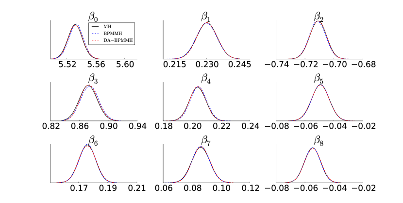
Figure 5.2. Kernel density estimations of marginal posteriors. The figure shows the marginal posteriors with the different algorithms MH (standard MH, solid black line), BPMMH (block PMMH, dashed blue line) and DA-BPMMH (delayed acceptance BPMMH, dashed red line). The approximations used by BPMMH for computing the likelihood estimate is based on $K=3.68$ (expressed as % of $n$) number of clusters with $\sigma^{2}\approx 10$. The delayed acceptance version uses an approximation based on $K^{(1)}=0.71$ (expressed as % of $n$) in the first stage.

6. Conclusions

We explore the use of the efficient and robust difference estimator in a delayed acceptance MH setting. The estimator incorporates auxiliary information about the contribution to the log-likelihood function while keeping the computational complexity low by operating on a sparse set of the data. We demonstrate that the estimator is more efficient than that of Payne and Mallick, (2015) in terms of having a much lower variance. Moreover, we prove that a lower variability implies that the delayed acceptance algorithm is more efficient, as measured by the probability of accepting the second stage conditional that the first stage is accepted. In an application to modeling of firm-bankruptcy, we find that the proposed delayed acceptance algorithm is feasible in the sense that it improves on the standard MH algorithm, which is sometimes not true for Payne and Mallick, (2015). We argue that previous approaches (discussed in the introduction) of exact simulation by MCMC are either (i) only possible under unfeasible assumptions or (ii) very inefficient (compared to MH). We therefore believe that exact simulation by subsampling MCMC is only possible by a delayed acceptance approach, and the implementation provided here is crucial for success.

Next, we realize that a delayed acceptance approach has the caveat of scanning the complete data when deciding upon final acceptance. We propose a state-dependent delayed acceptance that replaces the second stage evaluation with an estimate. This algorithm inherently allows for correlating the subsamples used for estimating the likelihood, and we can leverage on recent advances in the pseudo-marginal literature to reduce the computational cost. Moreover, we show that it is a special case of the state-dependent delayed acceptance in Christen and Fox, (2005) and thus convergence to an invariant distribution follows. This distribution is perturbed because the second stage estimate is biased, but we can control the error and ensure that it is within $O(m^{-2})$ of the true posterior. We demonstrate that the approximation is very accurate and we can improve on MH by a factor of $30$ in terms of a measure that balances statistical and computational efficiency.

Appendix A Proof of Theorem 1

Proof of Theorem 1.

It follows from the normality assumption that $X=R_{m}\sim\log\mathcal{N}(0,\sigma_{R}^{2})$ with density

$$f(x) = \frac{1}{x}\frac{1}{\sqrt{2\pi\sigma_{R}^{2}}}\exp\left(-\frac{1}{2\sigma_{R}^{2}}\log(x)^{2}\right),\quad x>0.$$

The expectation of the acceptance probability $\alpha_{2}(\theta_{c}\rightarrow\theta_{p})$ with respect to $X$ is

$$\mathrm{E}[\min(1,X)] = \int_{0}^{1}xf(x)dx+\int_{1}^{\infty}f(x)dx.$$

Since $\text{median}(X)=1$ we obtain $\int_{1}^{\infty}f(x)dx=0.5$. Now,

$$\int_{0}^{1}xf(x)dx = \int_{0}^{1}\frac{1}{\sqrt{2\pi\sigma_{R}^{2}}}\exp\left(-\frac{1}{2\sigma_{R}^{2}}\log(x)^{2}\right)dx$$

$$= \exp\left(\sigma_{R}^{2}/2\right)\int_{-\infty}^{0}\frac{1}{\sqrt{2\pi\sigma_{R}^{2}}}\exp\left(-\frac{1}{2\sigma_{R}^{2}}(y-\sigma_{R}^{2})^{2}\right)dy,$$

with $y=\log(x)$. The integrand is the pdf of $Y\sim\mathcal{N}(\sigma_{R}^{2},\sigma_{R}^{2})$ and thus

$$\mathrm{E}[\min(1,X)] = \exp\left(\sigma_{R}^{2}/2\right)\left(1-\Phi(\sigma_{R})\right)+0.5.$$

We now show that $\mathrm{E}[\min(1,X)]$ is decreasing in $\sigma_{R}$. We have that

$$\frac{d}{d\sigma_{R}}\mathrm{E}[\min(1,X)] = \exp\left(\sigma_{R}^{2}/2\right)\left(\sigma_{R}-\sigma_{R}\Phi(\sigma_{R})-\frac{1}{\sqrt{2\pi}}\right),$$

and we can (numerically) compute the maximum of the expression in brackets on the right which is $\approx-0.23$. Since $\exp\left(\sigma_{R}^{2}/2\right)>0$ it follows that $\frac{d}{d\sigma_{R}}\mathrm{E}[\min(1,X)]<0$ and hence $\mathrm{E}[\alpha_{2}(\theta_{c}\rightarrow\theta_{p})]$ decreases as a function of $\sigma_{R}$.

∎

References

- Andrieu and Roberts, (2009) Andrieu, C. and Roberts, G. O. (2009). The pseudo-marginal approach for efficient Monte Carlo computations. The Annals of Statistics, pages 697–725.
- Banterle et al., (2014) Banterle, M., Grazian, C., and Robert, C. P. (2014). Accelerating Metropolis-Hastings algorithms: Delayed acceptance with prefetching. arXiv preprint arXiv:1406.2660.
- Bardenet et al., (2014) Bardenet, R., Doucet, A., and Holmes, C. (2014). Towards scaling up Markov chain Monte Carlo: an adaptive subsampling approach. In Proceedings of The 31st International Conference on Machine Learning, pages 405–413.
- Bardenet et al., (2015) Bardenet, R., Doucet, A., and Holmes, C. (2015). On Markov chain Monte Carlo methods for tall data. arXiv preprint arXiv:1505.02827.
- Beaumont, (2003) Beaumont, M. A. (2003). Estimation of population growth or decline in genetically monitored populations. Genetics, 164(3):1139–1160.
- Ceperley and Dewing, (1999) Ceperley, D. and Dewing, M. (1999). The penalty method for random walks with uncertain energies. The Journal of Chemical Physics, 110(20):9812–9820.
- Christen and Fox, (2005) Christen, J. A. and Fox, C. (2005). MCMC using an approximation. Journal of Computational and Graphical Statistics, 14(4):795–810.
- Cui et al., (2011) Cui, T., Fox, C., and O’Sullivan, M. (2011). Bayesian calibration of a large-scale geothermal reservoir model by a new adaptive delayed acceptance Metropolis Hastings algorithm. Water Resources Research, 47(10).
- Deligiannidis et al., (2016) Deligiannidis, G., Doucet, A., and Pitt, M. K. (2016). The correlated pseudo-marginal method. arXiv preprint arXiv:1511.04992v3.
- Doucet et al., (2015) Doucet, A., Pitt, M., Deligiannidis, G., and Kohn, R. (2015). Efficient implementation of Markov chain Monte Carlo when using an unbiased likelihood estimator. Biometrika, 102(2):295–313.
- Fox and Nicholls, (1997) Fox, C. and Nicholls, G. (1997). Sampling conductivity images via MCMC. In Mardia, K., Gill, C., and Aykroyd, R., editors, The art and science of Bayesian image analysis, pages 91–100. Citeseer.
- Giordani et al., (2014) Giordani, P., Jacobson, T., Von Schedvin, E., and Villani, M. (2014). Taking the twists into account: Predicting firm bankruptcy risk with splines of financial ratios. Journal of Financial and Quantitative Analysis, 49(04):1071–1099.
- Golightly et al., (2015) Golightly, A., Henderson, D. A., and Sherlock, C. (2015). Delayed acceptance particle MCMC for exact inference in stochastic kinetic models. Statistics and Computing, 25(5):1039–1055.
- Hansen and Hurwitz, (1943) Hansen, M. H. and Hurwitz, W. N. (1943). On the theory of sampling from finite populations. The Annals of Mathematical Statistics, 14(4):333–362.
- Hastings, (1970) Hastings, W. K. (1970). Monte Carlo sampling methods using Markov chains and their applications. Biometrika, 57(1):97–109.
- Horvitz and Thompson, (1952) Horvitz, D. G. and Thompson, D. J. (1952). A generalization of sampling without replacement from a finite universe. Journal of the American Statistical Association, 47(260):663–685.
- Jacob and Thiery, (2015) Jacob, P. E. and Thiery, A. H. (2015). On nonnegative unbiased estimators. The Annals of Statistics, 43(2):769–784.
- Korattikara et al., (2014) Korattikara, A., Chen, Y., and Welling, M. (2014). Austerity in MCMC land: Cutting the Metropolis-Hastings budget. In Proceedings of the 31st International Conference on Machine Learning (ICML-14), pages 181–189.
- Liu, (2008) Liu, J. S. (2008). Monte Carlo strategies in scientific computing. Springer Science & Business Media.
- Lyne et al., (2015) Lyne, A.-M., Girolami, M., Atchade, Y., Strathmann, H., and Simpson, D. (2015). On Russian roulette estimates for Bayesian inference with doubly-intractable likelihoods. Statistical Science, 30(4):443–467.
- Maclaurin and Adams, (2014) Maclaurin, D. and Adams, R. P. (2014). Firefly Monte Carlo: Exact MCMC with subsets of data. In Proceedings of the 30th Conference on Uncertainty in Artificial Intelligence (UAI 2014).
- Maire et al., (2015) Maire, F., Friel, N., and Alquier, P. (2015). Light and widely applicable MCMC: Approximate Bayesian inference for large datasets. arXiv preprint arXiv:1503.04178.
- Metropolis et al., (1953) Metropolis, N., Rosenbluth, A. W., Rosenbluth, M. N., Teller, A. H., and Teller, E. (1953). Equation of state calculations by fast computing machines. The Journal of Chemical Physics, 21(6):1087–1092.
- Minsker et al., (2014) Minsker, S., Srivastava, S., Lin, L., and Dunson, D. (2014). Scalable and robust Bayesian inference via the median posterior. In Proceedings of the 31st International Conference on Machine Learning (ICML-14), pages 1656–1664.
- Neiswanger et al., (2013) Neiswanger, W., Wang, C., and Xing, E. (2013). Asymptotically exact, embarrassingly parallel MCMC. arXiv preprint arXiv:1311.4780.
- Nemeth and Sherlock, (2016) Nemeth, C. and Sherlock, C. (2016). Merging MCMC subposteriors through Gaussian-process approximations. arXiv preprint arXiv:1605.08576.
- Nicholls et al., (2012) Nicholls, G. K., Fox, C., and Watt, A. M. (2012). Coupled MCMC with a randomized acceptance probability. arXiv preprint arXiv:1205.6857.
- Payne and Mallick, (2015) Payne, R. D. and Mallick, B. K. (2015). Bayesian big data classification: A review with complements. arXiv preprint arXiv:1411.5653v2.
- Pitt et al., (2012) Pitt, M. K., Silva, R. d. S., Giordani, P., and Kohn, R. (2012). On some properties of Markov chain Monte Carlo simulation methods based on the particle filter. Journal of Econometrics, 171(2):134–151.
- Plummer et al., (2006) Plummer, M., Best, N., Cowles, K., and Vines, K. (2006). Coda: Convergence diagnosis and output analysis for MCMC. R News, 6(1):7–11.
- Quiroz et al., (2017) Quiroz, M., Tran, M.-N., Villani, M., and Kohn, R. (2017). Exact subsampling MCMC. arXiv preprint arXiv:1603.08232.
- Quiroz et al., (2016) Quiroz, M., Villani, M., Kohn, R., and Tran, M.-N. (2016). Speeding up MCMC by efficient data subsampling. arXiv preprint arXiv:1404.4178v4.
- Rhee and Glynn, (2015) Rhee, C. and Glynn, P. W. (2015). Unbiased estimation with square root convergence for SDE models. Operations Research, 63(5):1026–1043.
- Roberts et al., (1997) Roberts, G. O., Gelman, A., and Gilks, W. R. (1997). Weak convergence and optimal scaling of random walk Metropolis algorithms. The Annals of Applied Probability, 7(1):110–120.
- Särndal et al., (2003) Särndal, C.-E., Swensson, B., and Wretman, J. (2003). Model assisted survey sampling. Springer.
- Scott et al., (2013) Scott, S. L., Blocker, A. W., Bonassi, F. V., Chipman, H., George, E., and McCulloch, R. (2013). Bayes and big data: the consensus Monte Carlo algorithm. In EFaBBayes 250” conference, volume 16.
- (37) Sherlock, C., Golightly, A., and Henderson, D. A. (2015a). Adaptive, delayed-acceptance MCMC for targets with expensive likelihoods. arXiv preprint arXiv:1509.00172.
- (38) Sherlock, C., Thiery, A., and Golightly, A. (2015b). Efficiency of delayed-acceptance random walk Metropolis algorithms. arXiv preprint arXiv:1506.08155.
- (39) Sherlock, C., Thiery, A. H., Roberts, G. O., and Rosenthal, J. S. (2015c). On the efficiency of pseudo-marginal random walk Metropolis algorithms. The Annals of Statistics, 43(1):238–275.
- Smith, (2011) Smith, M. (2011). Estimating nonlinear economic models using surrogate transitions. Federal Reserve Board, Manuscript. https://www.economicdynamics.org/meetpapers/2012/paper_494.pdf.
- Solonen et al., (2012) Solonen, A., Ollinaho, P., Laine, M., Haario, H., Tamminen, J., Järvinen, H., et al. (2012). Efficient MCMC for climate model parameter estimation: Parallel adaptive chains and early rejection. Bayesian Analysis, 7(3):715–736.
- Tran et al., (2016) Tran, M.-N., Kohn, R., Quiroz, M., and Villani, M. (2016). Block-wise pseudo-marginal Metropolis-Hastings. arXiv preprint arXiv:1603.02485v3.
- Wang and Dunson, (2013) Wang, X. and Dunson, D. B. (2013). Parallel MCMC via Weierstrass sampler. arXiv preprint arXiv:1312.4605.