Generation and complete nondestructive analysis of hyperentanglement assisted by nitrogen-vacancy centers in resonators

Abstract

We present two efficient schemes for the deterministic generation and the complete nondestructive analysis of hyperentangled Bell states in both the polarization and spatial-mode degrees of freedom (DOFs) of two-photon systems, assisted by the nitrogen-vacancy (NV) centers in diamonds coupled to microtoroidal resonators as a result of cavity quantum electrodynamics (QED). With the input-output process of photons, two-photon polarization-spatial hyperentangled Bell states can be generated in a deterministic way and their complete nondestructive analysis can be achieved. These schemes can be generalized to generate and analyze hyperentangled Greenberger-Horne-Zeilinger states of multi-photon systems as well. Compared with previous works, these two schemes relax the difficulty of their implementation in experiment as it is not difficult to obtain the $\pi$ phase shift in single-sided NV-cavity systems. Moreover, our schemes do not require that the transmission for the uncoupled cavity is balanceable with the reflectance for the coupled cavity. Our calculations show that these schemes can reach a high fidelity and efficiency with current technology, which may be a benefit to long-distance high-capacity quantum communication with two DOFs of photon systems.

I Introduction

Recently, hyperentanglement, which is defined as the entanglement in multiple degrees of freedom (DOFs) of a quantum system heper1 ; heper2 ; heper3 , has attracted much attention as it has some important applications in quantum information processing. It can speedup quantum computation (e.g., hyper-parallel photonic quantum computation hypercomputation ; hypercomputation2 ) and it can be used to assist the complete Bell-state analysis and entanglement purification. In 2003, Walborn et al. Walborn presented a simple linear-optical scheme for the complete Bell-state analysis of photons with hyperentanglement. In 2006, Schuck et al. Schuck demonstrated the complete deterministic analysis of polarization Bell states with only linear optics assisted by polarization-time-bin hyperentanglement. In 2007, Barbieri et al. Barbieri demonstrated the complete and deterministic discrimination of polarization Bell states assisted by momentum entanglement. In 2009, Wilde and Uskov quantumec proposed a quantum-error-correcting-code scheme assisted by linear-optical hyperentanglement. In 2010, some deterministic entanglement purification protocols (EPPs) EPPsheng2 ; EPPsheng3 ; EPPdeng were proposed with the polarization-spatial hyperentanglement of photon systems, which can solve the troublesome problem that a large amount of quantum resources would be sacrificed in the conventional EPPs, and they are very useful in practical quantum repeaters. In 2012, Wang, Song, and Long repeater4 proposed an important quantum repeater protocol with polarization-spatial hyperentanglement.

The hyperentanglement of photon systems can also be used to largely increase the channel capacity of quantum communication. For example, Barreiro et al. HESC beat the channel capacity limit of photonic superdense coding with polarization-orbital-angular-momentum hyperentanglement in linear optics in 2008. In 2010, Sheng, Deng, and Long kerr gave the first scheme for the complete hyperentangled-Bell-state analysis (HBSA) for quantum communication, and they designed the pioneering model for the quantum teleportation with two DOFs of photon pairs, resorting to cross-Kerr nonlinearity. In 2011, Pisenti et al. HBSA1 pointed out the limitations for manipulation and measurement of entangled systems with inherently linear unentangling devices. In 2012, Ren et al. HBSA2 proposed another interesting scheme for the complete HBSA for photon systems by using the giant nonlinear optics in quantum dot-cavity systems and they presented the entanglement swapping with photonic polarization-spatial hyperentanglement. In 2012, Wang, Lu, and Long HBSA3 introduced an interesting scheme for the complete HBSA for photon systems by the giant circular birefringence induced by double-sided quantum-dot-cavity systems. In 2013, Ren, Du, and Deng HECP proposed the parameter-splitting method to extract the polarization-spatial maximally hyerentangled photons when the coefficients of the initial partially hyperentangled states are known, and this fascinating method can be achieved with the maximum success probability by performing the protocol only once, resorting to linear-optical elements only. They HECP also gave the first hyperentanglement concentration protocol (hyper-ECP) for unknown polarization-spatial less-hyperentangled states with linear-optical elements only HECP . Ren and Deng HyperEPP presented the first hyperentanglement purification protocol (hyper-EPP) for two-photon systems in polarization-spatial hyperentangled states, and it is very useful in the high-capacity quantum repeaters with hyperentanglement. In 2014, Ren, Du, and Deng RenHEPP2 gave a two-step hyper-EPP for polarization-spatial hyperentangled states with the quantum-state-joining method, and it has a far higher efficiency. In the same time, Ren and Long hyperecpgeneral proposed a general hyper-ECP for photon systems assisted by quantum dot spins inside optical microcavities. Recently, Li and Ghose presented an interesting hyper-ECP resorting to linear optics lixhyperconcentration and another efficient hyper-ECP for the multipartite hyperentangled state via the cross-Kerr nonlinearity lixhyperconcentration2 .

Another attractive candidate for solid-state quantum information processing is the nitrogen-vacancy (NV) center in a diamond, owing to its long decoherence time even at room temperature Jelezko , and its spin can be initialized and readout via a highly stable optical transition Davies ; Gruber . By using the coherent manipulation of an electron spin and nearby individual nuclear spins, Dutt et al. register demonstrated a controllable quantum register in NV centers in 2007. Decoherence-protected quantum gates for a hybrid solid-state register register1 was also experimentally demonstrated on a single NV center. As this system allows for high-fidelity polarization and detection of single electron and nuclear spin states even under ambient conditions PD1 ; PD2 ; Gruber ; PD3 , the multipartite entanglement among single spins in diamond was demonstrated by Neumann et al. Neumann in 2008. In 2010, Togan et al. QEG realized the quantum entanglement generation of an optical photon and an NV center. Photon Fock states on-demand can be implemented in a low-temperature solid-state quantum system with an NV center in a nano-diamond coupled to a nearby high-Q optical cavity Fock .

Recently, a combination of NV centers and microcavities, a promising solid-state cavity quantum electrodynamics (QED) system, has gained widespread attention transfer ; s33 ; s34 ; s35 ; s36 ; s37 ; s38 ; WeigateNV ; wang . One of the microcavities is called microtoroidal resonator (MTR) with a quantized whispering-gallery mode (WGM) and required to be of a high Q factor and a small mode volume MTR1 ; MTR2 . However, when MTR couples to a fiber, its Q factor is surely degraded s34 . The single-photon input-output process from a MTR in experiment also has been demonstrated s34 . In 2009, the quantum nondemolition measurement on a single spin of an NV center has been proposed with a low error rate s37 and it was experimentally demonstrated through Faraday rotation s38 in 2010. In 2011, Chen et al. s36 proposed an efficient scheme to entangle separate NV centers by coupling to MTRs. In 2013, Wei and Deng WeigateNV proposed some interesting schemes for compact quantum gates on electron-spin qubits assisted by diamond NV centers inside cavities.

In this paper, we present two efficient schemes to generate deterministically hyperentangled states, i.e., hyperentangled Bell states and hyperentangled Greenberger-Horne-Zeilinger (GHZ) states, in which photons are entangled in both the polarization and spatial-mode DOFs, assisted by the NV centers in diamonds coupled to MTRs and the input-output process of photons as a result of cavity QED. We also propose a scheme to distinguish completely the 16 polarization-spatial hyperentangled Bell states, and it works in a nondestructive way. After analyzing the hyperentangled Bell states, the photon systems can be used for other tasks in quantum information processing. Compared with previous works kerr ; HBSA2 ; HBSA3 , these two schemes relax the difficulty of their implementation in experiment as it is not difficult to obtain the $\pi$ phase shift in single-sided NV-cavity systems. Moreover, they do not require that the transmission for the uncoupled cavity is balanceable with the reflectance for the coupled cavity. Our calculations show that these schemes can work with a high fidelity and efficiency with current experimental techniques, which may be beneficial to long-distance high-capacity quantum communication, such as quantum teleportation, quantum dense coding, and quantum superdense coding with two DOFs of photon systems.

This article is organized as follows. In Sec. II, we will introduce the diamond-NV-center system and its single-photon input-output process. The generation of hyperentangled Bell states and hyperentangled GHZ states, and the complete nondestructive HBSA are presented in Secs. III and IV. A discussion and a summary are given in Sec. V.

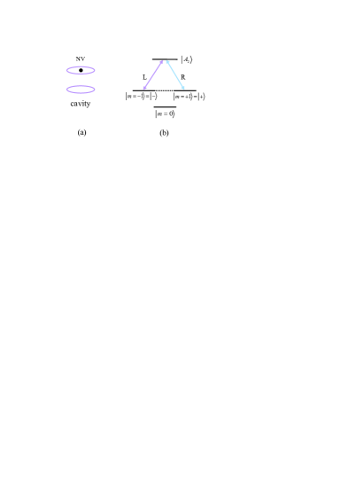
Figure 1: (Color online) (a) Schematic diagram for an NV center inside an MTR. (b) The electron energy-level configuration of an NV center in an MTR with the relevant transitions driven by different polarized photons. $L$ ($R$) represents the left(right) circularly polarized photon.

II A nitrogen-vacancy center in microtoroidal resonator

As shown in Fig. 1(a), an NV center, composed of a substitutional nitrogen atom and an adjacent vacancy in diamond lattice, is coupled to an MTR with a WGM. The NV center is negatively charged with two unpaired electrons located at the vacancy, and the energy-level structure of the NV center coupling to the cavity mode is shown in Fig. 1(b). The ground state is a spin triplet with the splitting at $2.87$ GHz between the levels $|m=0\rangle$ and $|m=\pm 1\rangle$ owing to spin-spin interactions. The specifically excited state, which is one of the six eigenstates of the full Hamitonian including spin-orbit and spin-spin interactions in the absence of any perturbation, such as by an external magnetic field or crystal strain, is labeled as QEG $|A_{2}\rangle=|E_{-}\rangle|+\rangle+|E_{+}\rangle|-\rangle$, where $|E_{+}\rangle$ and $|E_{-}\rangle$ are the orbital states with the angular momentum projections $+1$ and $-1$ along the NV axis, respectively. The optical transition is allowed between the ground state $|m=\pm 1\rangle$ and the excited state $|A_{2}\rangle$ owing to the total angular momentum conservation QEG ; Lenef .

An NV center can be modeled as a $\Lambda$-type three-level structure with the ground state $|-\rangle=|m=-1\rangle$ and $|+\rangle=|m=1\rangle$, and the excited state is $|1\rangle=|A_{2}\rangle$. The transitions $|-\rangle\leftrightarrow|1\rangle$ and $|+\rangle\leftrightarrow|1\rangle$ in the NV center are resonantly coupled to the right (R) and the left (L) circularly polarized photons with the identical transition frequency, respectively. Considering the structure in Fig.1, which can be modeled as a single-sided cavity, one can write down the Heisenberg equations of motion for this system as follows:

$$\begin{split}\frac{da}{dt}&=-[i(\omega_{c}-\omega)+\frac{\kappa}{2}+\frac{\kappa_{s}}{2}]\,a-\text{g}\sigma_{\!-}-\sqrt{\kappa}\,a_{in},\\ \frac{d\sigma_{\!-}}{dt}&=-[i(\omega_{0}-\omega)+\frac{\gamma}{2}]\sigma_{\!-}-\text{g}\sigma_{\!z}a,\\ a_{out}&=a_{in}+\sqrt{\kappa}\,a,\end{split}$$ (1)

where $\omega$, $\omega_{c}$, and $\omega_{0}$ are the frequencies of the photon, cavity mode, and the atomic-level transition, respectively. g is the coupling strength between the NV center and the cavity mode. $\frac{\gamma}{2}$ and $\frac{\kappa}{2}$ are the decay rates of the NV center and the cavity field, respectively. $\frac{\kappa_{s}}{2}$ is the side leakage rate of the cavity. $a_{in}$ and $a_{out}$ are the input and the output field operators.

In the weak excitation approximation, the reflection coefficient in the steady state can be obtained,

$$r(\omega)=1-\frac{\kappa[i(\omega_{0}-\omega)+\frac{\gamma}{2}]}{[i(\omega_{0}-\omega)+\frac{\gamma}{2}][i(\omega_{c}-\omega)+\frac{\kappa}{2}+\frac{\kappa_{s}}{2}]+\text{g}^{2}}.$$

For $\text{g}=0$, the reflection coefficient $r_{0}(\omega)$ is

$$r_{0}(\omega)=\frac{i(\omega_{c}-\omega)-\frac{\kappa}{2}+\frac{\kappa_{s}}{2}}{i(\omega_{c}-\omega)+\frac{\kappa}{2}+\frac{\kappa_{s}}{2}}.$$ (3)

From Eqs. (II) and (3), one can see that if $\omega_{0}=\omega_{c}=\omega$,

$$r(\omega)=\frac{(\kappa_{s}-\kappa)\gamma+4\text{g}^{2}}{(\kappa_{s}+\kappa)\gamma+4\text{g}^{2}},\;\;\;\;\;\;\;\;r_{0}(\omega)=\frac{\kappa_{s}-\kappa}{\kappa_{s}+\kappa}.$$ (4)

If the NV center is in the initial state $|-\rangle$ ($|+\rangle$) and a single polarized photon $|L\rangle$ ($|R\rangle$) is input, the photon will experience a phase shift $e^{i\phi}$ owing to the Faraday rotation. However, if the initial state of the NV center is $|-\rangle$ ($|+\rangle$), the input photon with $|R\rangle$ ($|L\rangle$) polarization will get a phase shift $e^{i\phi_{0}}$. In the resonant condition $\omega_{0}=\omega_{c}=\omega$, when $\kappa_{s}\ll\kappa$ and $4\text{g}^{2}\gg\kappa\gamma$, we approximately have $\phi=0$ and $\phi_{0}=\pi$ from Eq. (II). The change of the input photon can be summarized as follows WeigateNV :

$$|R\rangle|+\rangle \rightarrow |R\rangle|+\rangle,\;\;\;\;\;\;\,|R\rangle|-\rangle\;\rightarrow\;-|R\rangle|-\rangle,$$

$$|L\rangle|+\rangle \rightarrow -|L\rangle|+\rangle,\;\;\;\;|L\rangle|-\rangle\;\rightarrow\;|L\rangle|-\rangle.$$ (5)

III Photonic hyperentanglement generation

We first describe how to generate two-photon polarization-spatial hyperentangled Bell states assisted by NV centers coupled to MTRs as a result of cavity QED, and then extend this approach for the generation of three-photon polarization-spatial hyperentangled GHZ states.

III.1 Generation of two-photon hyperentangled Bell states

A two-photon hyperentangled Bell state in both the polarization and the spatial-mode DOFs can be expressed as

$$|\eta_{1}^{+}\rangle_{PS}=\frac{1}{2}(|RR\rangle+|LL\rangle)_{ab}(|a_{1}b_{1}\rangle+|a_{2}b_{2}\rangle)_{ab}.$$ (6)

Here, $|R\rangle$ and $|L\rangle$ denote the right-circular polarization and the left-circular polarization of photons, respectively. $a_{1}$ ($b_{1}$) and $a_{2}$ ($b_{2}$) are the different spatial modes for photon $a$ (b). The subscripts $P$ and $S$ denote the polarization and the spatial-mode DOFs, respectively. $a$ and $b$ represent the two photons in the hyperentangled state. The four Bell states in the polarization DOF can be expressed as

$$\begin{split}|\Phi_{1}^{\pm}\rangle_{P}&=\frac{1}{\sqrt{2}}(|RR\rangle\pm|LL\rangle),\\ |\Phi_{2}^{\pm}\rangle_{P}&=\frac{1}{\sqrt{2}}(|LR\rangle\pm|RL\rangle),\end{split}$$ (7)

and those in the spatial-mode DOF can be written as

$$\begin{split}|\Phi_{1}^{\pm}\rangle_{S}&=\frac{1}{\sqrt{2}}(|a_{1}b_{1}\rangle\pm|a_{2}b_{2}\rangle),\\ |\Phi_{2}^{\pm}\rangle_{S}&=\frac{1}{\sqrt{2}}(|a_{2}b_{1}\rangle\pm|a_{1}b_{2}\rangle).\end{split}$$ (8)

The principle of our scheme for the two-photon polarization-spatial hyperentangled Bell states generation (HBSG) assisted by NV centers coupled to MTRs as a result of cavity QED is shown in Fig.2. Here SW is an optical switch and BS represents a $50:50$ beam splitter which can accomplish the following transformation in the spatial-mode DOF of the photons,

$$\begin{split}K_{a_{1}(b_{2})}^{{\dagger}}&\rightarrow\frac{1}{\sqrt{2}}(K_{c_{1}(d_{1})}^{{\dagger}}+K_{c_{2}(d_{2})}^{{\dagger}}),\\ K_{a_{2}(b_{1})}^{{\dagger}}&\rightarrow\frac{1}{\sqrt{2}}(K_{c_{1}(d_{1})}^{{\dagger}}-K_{c_{2}(d_{2})}^{{\dagger}}).\end{split}$$ (9)

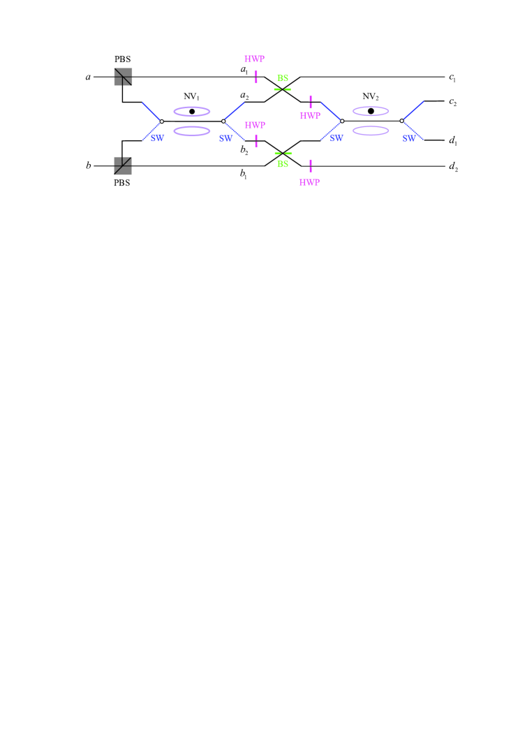
Figure 2: (Color online) Schematic diagram for two-photon polarization-spatial HBSG. PBS represents a circular polarization beam splitter which is used to transmit the $L$ polarized photon and reflect the $R$ polarized photon, respectively. SW represents an optical switch and BS is a 50:50 beam splitter. HWP represents a half-wave plate which is used to perform a bit-flip operation $X=|R\rangle\langle L|+|L\rangle\langle R|$ on the photon in the polarization DOF. NV₁ and NV₂ represent two NV centers. $k_{1}$ and $k_{2}$ ($k=a,b,c,d$) represent different spatial modes.

Suppose that two NV centers NV₁ and NV₂ are initialed to the superposition states $|\varphi^{+}\rangle_{1}=|\varphi^{+}\rangle_{2}=\frac{1}{\sqrt{2}}(|-\rangle+|+\rangle)$, and the two photons $a$ and $b$ with the same frequency are prepared in the same initial state $|\phi\rangle_{a}=|\phi\rangle_{b}=\frac{1}{\sqrt{2}}(|R\rangle+|L\rangle)$. Photons $a$ and $b$ are successively sent into the device shown in Fig.2. A time interval $\Delta t$ exists between two photons, and $\Delta t$ should be less than the spin coherence time $T$. When photon $a$ passes through the cavity, the optical switch (SW) is switched to await photon $b$. After passing through the two NV centers, the two photons $a$ and $b$ can be entangled with the electron spins in the NV centers in the two cavities. The corresponding transformations on the states can be described as follows:

$$\!\!|\Phi\rangle_{0}\!\!\!\! = \!\!|\phi\rangle_{a}|\phi\rangle_{b}|\varphi^{+}\rangle_{1}|\varphi^{+}\rangle_{2}$$ (10)

$$\xrightarrow{P\!B\!S\!s} \!\!\!\frac{1}{2}(|L\rangle|a_{1}\!\rangle\!+\!|R\rangle|a_{2}\!\rangle)(|L\rangle|b_{1}\!\rangle\!+\!|R\rangle|b_{2}\!\rangle)|\varphi^{+}\!\rangle_{1}|\varphi^{+}\!\rangle_{2},$$

$$\!\!\!\!\xrightarrow{NV_{1}} \!\!\!\frac{1}{2}[(|LL\rangle|a_{1}b_{1}\rangle+|RR\rangle|a_{2}b_{2}\rangle)|\varphi^{+}\rangle_{1}$$

$$-(|LR\rangle|a_{1}b_{2}\rangle+|RL\rangle|a_{2}b_{1}\rangle)|\varphi^{-}\rangle_{1}]|\varphi^{+}\rangle_{2},$$

$$\!\!\!\!\xrightarrow{B\!S} \!\!\!\frac{1}{4}[|\Phi_{1}^{+}\rangle_{P}|\Phi_{1}^{-}\rangle_{S}|\varphi^{+}\rangle_{1}+|\Phi_{1}^{-}\rangle_{P}|\Phi_{2}^{-}\rangle_{S}|\varphi^{+}\rangle_{1}$$

$$-|\Phi_{2}^{+}\rangle_{P}|\Phi_{1}^{+}\rangle_{S}|\varphi^{-}\!\rangle_{1}\!+\!|\Phi_{2}^{-}\rangle_{P}|\Phi_{2}^{+}\rangle_{S}|\varphi^{-}\!\rangle_{1}]|\varphi^{+}\!\rangle_{2},$$

$$\!\!\!\!\xrightarrow{NV_{2}\;} \!\!\!\frac{1}{4}(-|\Phi_{1}^{-}\rangle_{P}|\Phi_{1}^{-}\rangle_{S}|\varphi^{+}\rangle_{1}|\varphi^{-}\rangle_{2}$$

$$+\,|\Phi_{1}^{-}\rangle_{P}|\Phi_{2}^{-}\rangle_{S}|\varphi^{+}\rangle_{1}|\varphi^{+}\rangle_{2}$$

$$+\,|\Phi_{2}^{-}\rangle_{P}|\Phi_{1}^{-}\rangle_{S}|\varphi^{-}\rangle_{1}|\varphi^{-}\rangle_{2}$$

$$+\,|\Phi_{2}^{-}\rangle_{P}|\Phi_{2}^{-}\rangle_{S}|\varphi^{-}\rangle_{1}|\varphi^{+}\rangle_{2}).$$

Here $|\varphi^{\pm}\rangle=\frac{1}{\sqrt{2}}(|-\rangle\pm|+\rangle)$.

From Eq. (10), one can see that the injecting photons $a$ and $b$ pass through PBS in sequence. Each of them is split into two wave-packets. The part of photon $a$ ($b$) in the state $|L\rangle$ is transmitted to path $a_{1}$ ($b_{1}$), while the part in the state $|R\rangle$ is reflected by PBS to path $a_{2}$ ($b_{2}$) and subsequently it interacts with the first NV center (named NV₁). The wave-packets from the spatial modes $a_{1}$ and $a_{2}$ ($b_{1}$ and $b_{2}$) are mixed at the beam splitter (BS). HWP is used to keep the polarization state of the photon unchanged. After BSs, the states of the two-photon systems are divided into two groups, according to the state of NV₂ when it is measured with the basis $\{|\varphi^{+}\rangle,|\varphi^{-}\rangle\}$. So do the outcomes of the measurement on NV₁. The relationship between the measurement outcomes of these two NV centers and the polarization-spatial hyperentangled Bell states of the two photons is shown in Table 1.

Table 1: The relation between the outcomes of the two NV centers and the final polarization-spatial hyperentangled Bell states.

NV1	NV2	hyperentangled Bell states
$|\varphi^{+}\rangle_{1}$	$|\varphi^{-}\rangle_{2}$	$|\Phi_{1}^{-}\rangle_{P}|\Phi_{1}^{-}\rangle_{S}$
$|\varphi^{+}\rangle_{1}$	$|\varphi^{+}\rangle_{2}$	$|\Phi_{1}^{-}\rangle_{P}|\Phi_{2}^{-}\rangle_{S}$
$|\varphi^{-}\rangle_{1}$	$|\varphi^{-}\rangle_{2}$	$|\Phi_{2}^{-}\rangle_{P}|\Phi_{1}^{-}\rangle_{S}$
$|\varphi^{-}\rangle_{1}$	$|\varphi^{+}\rangle_{2}$	$|\Phi_{2}^{-}\rangle_{P}|\Phi_{2}^{-}\rangle_{S}$

From Table 1, one can see that if NV₁ is in the state $|\varphi^{+}\rangle_{1}$ and NV₂ is in the state $|\varphi^{-}\rangle_{2}$, the two-photon system $ab$ is in the hyperentangled Bell state $|\Phi_{1}^{-}\rangle_{P}|\Phi_{1}^{-}\rangle_{S}$. When the two NV centers are in the states $|\varphi^{+}\rangle_{1}$ and $|\varphi^{+}\rangle_{2}$, respectively, the two-photon system is in the hyperentangled Bell state $|\Phi_{1}^{-}\rangle_{P}|\Phi_{2}^{-}\rangle_{S}$. The hyperentangled Bell states $|\Phi_{2}^{-}\rangle_{P}|\Phi_{1}^{-}\rangle_{S}$ and $|\Phi_{2}^{-}\rangle_{P}|\Phi_{2}^{-}\rangle_{S}$ also correspond to different combinations of the states of the two NV centers. Therefore, one can generate the polarization-spatial hyperentangled Bell states of the two-photon system by measuring the states of the two NV centers. By applying a Hadamard operation on the electron-spin state, its states $\frac{1}{\sqrt{2}}(|-\rangle+|+\rangle)$ and $\frac{1}{\sqrt{2}}(|-\rangle-|+\rangle)$ can be rotated to $|+\rangle$ and $|-\rangle$, respectively. The measurement on spin readout can be achieved with the resonant optical excitation Gaebel . Other polarization-spatial hyperentangled Bell states can be obtained in a similar way or by resorting to the single-qubit operations and the acquired hyperentangled Bell state.

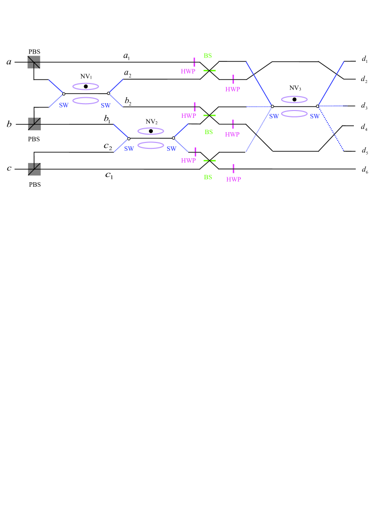
Figure 3: (Color online) Schematic diagram for the generation of three-photon polarization-spatial hyperentangled GHZ states.

III.2 Generation of three-photon hyperentangled GHZ states

Similar to the case for two-photon polarization-spatial hyperentangled Bell states, we denote a three-photon polarization-spatial hyperentangled GHZ state as

$$|\zeta_{1}^{+}\rangle_{PS}=\frac{1}{2}(|RRR\rangle\!+\!|LLL\rangle)_{abc}(|a_{1}b_{1}c_{1}\rangle\!+\!|a_{2}b_{2}c_{2}\rangle)_{abc}.$$

Here $a$, $b$, and $c$ represent the three photons in the hyperentangled state. The eight three-photon GHZ states in the polarization DOF can be expressed as

$$\begin{split}|\Psi_{1}^{\pm}\rangle_{P}&=\frac{1}{\sqrt{2}}(|RRR\rangle\pm|LLL\rangle),\\ |\Psi_{2}^{\pm}\rangle_{P}&=\frac{1}{\sqrt{2}}(|LRR\rangle\pm|RLL\rangle),\\ |\Psi_{3}^{\pm}\rangle_{P}&=\frac{1}{\sqrt{2}}(|RLR\rangle\pm|LRL\rangle),\\ |\Psi_{4}^{\pm}\rangle_{P}&=\frac{1}{\sqrt{2}}(|RRL\rangle\pm|LLR\rangle).\end{split}$$ (12)

and the eight GHZ states in the spatial-mode DOF are

$$\begin{split}|\Psi_{1}^{\pm}\rangle_{S}&=\frac{1}{\sqrt{2}}(|a_{1}b_{1}c_{1}\rangle\pm|a_{2}b_{2}c_{2}\rangle),\\ |\Psi_{2}^{\pm}\rangle_{S}&=\frac{1}{\sqrt{2}}(|a_{2}b_{1}c_{1}\rangle\pm|a_{1}b_{2}c_{2}\rangle),\\ |\Psi_{3}^{\pm}\rangle_{S}&=\frac{1}{\sqrt{2}}(|a_{1}b_{2}c_{1}\rangle\pm|a_{2}b_{1}c_{2}\rangle),\\ |\Psi_{4}^{\pm}\rangle_{S}&=\frac{1}{\sqrt{2}}(|a_{1}b_{1}c_{2}\rangle\pm|a_{2}b_{2}c_{1}\rangle).\end{split}$$ (13)

The principle of our scheme for the generation of a three-photon polarization-spatial hyperentangled GHZ state is shown in Fig.3. Considering all the three NV centers are in the initial state $|\varphi^{+}\rangle_{1}=|\varphi^{+}\rangle_{2}=|\varphi^{+}\rangle_{3}=\frac{1}{\sqrt{2}}(|-\rangle+|+\rangle)$, and the flying photons $a$, $b$, and $c$ are in the superposition state $|\phi\rangle_{a}=|\phi\rangle_{b}=|\phi\rangle_{c}=\frac{1}{\sqrt{2}}(|R\rangle+|L\rangle)$. A brief description of our scheme for hyperentangled-GHZ-state generation can be written as follows.

Each of the three photons $a$, $b$, and $c$ is split into two wave-packets by PBS. The photon in the state $|L\rangle$ is injected into the pathes $a_{1}$, $b_{1}$, and $c_{1}$, while the photon in the state $|R\rangle$ is sent into the pathes $a_{2}$, $b_{2}$, and $c_{2}$. The photons in the pathes $a_{2}$ and $b_{2}$ interact with NV₁, and those in the pathes $b_{1}$ and $c_{2}$ interact with NV₂. BSs mix the spatial modes $a_{1}$ and $a_{2}$, $b_{1}$ and $b_{2}$, and $c_{1}$ and $c_{2}$. The states of the three photons are divided into four groups, according to the states of NV₁ and NV₂. Under the condition that NV₃ is imported, the hyperentangled states of the photons can be determined by measuring the states of the NV centers. The evolution of the whole system can be described as

$$|\Psi\rangle_{0}\!\!\!\! = \!\!|\phi\rangle_{a}|\phi\rangle_{b}|\phi\rangle_{c}|\varphi^{+}\rangle_{1}|\varphi^{+}\rangle_{2}|\varphi^{+}\rangle_{3}$$ (14)

$$\xrightarrow{U_{T}} \!\!\frac{1}{2\sqrt{2}}(|\Psi_{1}^{+}\rangle_{P}|\Psi_{2}^{+}\rangle_{S})|\varphi^{+}\rangle_{1}|\varphi^{-}\rangle_{2}|\varphi^{-}\rangle_{3}$$

$$-|\Psi_{1}^{+}\rangle_{P}|\Psi_{2}^{-}\rangle_{S}|\varphi^{+}\rangle_{1}|\varphi^{-}\rangle_{2}|\varphi^{+}\rangle_{3}$$

$$+|\Psi_{4}^{+}\rangle_{P}|\Psi_{2}^{+}\rangle_{S}|\varphi^{+}\rangle_{1}|\varphi^{+}\rangle_{2}|\varphi^{-}\rangle_{3}$$

$$+|\Psi_{4}^{+}\rangle_{P}|\Psi_{2}^{-}\rangle_{S}|\varphi^{+}\rangle_{1}|\varphi^{+}\rangle_{2}|\varphi^{+}\rangle_{3}$$

$$+|\Psi_{3}^{+}\rangle_{P}|\Psi_{2}^{+}\rangle_{S}|\varphi^{-}\rangle_{1}|\varphi^{+}\rangle_{2}|\varphi^{-}\rangle_{3}$$

$$-|\Psi_{3}^{+}\rangle_{P}|\Psi_{2}^{-}\rangle_{S}|\varphi^{-}\rangle_{1}|\varphi^{+}\rangle_{2}|\varphi^{+}\rangle_{3}$$

$$+|\Psi_{2}^{+}\rangle_{P}|\Psi_{1}^{+}\rangle_{S}|\varphi^{-}\rangle_{1}|\varphi^{-}\rangle_{2}|\varphi^{-}\rangle_{3}$$

$$-|\Psi_{2}^{+}\rangle_{P}|\Psi_{2}^{-}\rangle_{S}|\varphi^{-}\rangle_{1}|\varphi^{-}\rangle_{2}|\varphi^{+}\rangle_{3}).$$

Here $U_{T}$ represents the total operation by PBS, NV₁, NV₂, BS, and NV₃ in sequence. $|\varphi^{\pm}\rangle=\frac{1}{\sqrt{2}}(|-\rangle\pm|+\rangle)$. The relation between the outcomes of the measurements on the three NV centers and the obtained final polarization-spatial hyperentangled GHZ states is shown in Table 2.

Table 2: The relation between the outcomes of the three NV centers and the final hyperentangled GHZ states

NV1	NV2	NV3	hyperentangled GHZ states
$|\varphi^{+}\rangle_{1}$	$|\varphi^{-}\rangle_{2}$	$|\varphi^{-}\rangle_{3}$	$|\Psi_{1}^{+}\rangle_{P}|\Psi_{2}^{+}\rangle_{S}$
$|\varphi^{+}\rangle_{1}$	$|\varphi^{-}\rangle_{2}$	$|\varphi^{+}\rangle_{3}$	$|\Psi_{1}^{+}\rangle_{P}|\Psi_{2}^{-}\rangle_{S}$
$|\varphi^{+}\rangle_{1}$	$|\varphi^{+}\rangle_{2}$	$|\varphi^{-}\rangle_{3}$	$|\Psi_{4}^{+}\rangle_{P}|\Psi_{2}^{+}\rangle_{S}$
$|\varphi^{+}\rangle_{1}$	$|\varphi^{+}\rangle_{2}$	$|\varphi^{+}\rangle_{3}$	$|\Psi_{4}^{+}\rangle_{P}|\Psi_{2}^{-}\rangle_{S}$
$|\varphi^{-}\rangle_{1}$	$|\varphi^{+}\rangle_{2}$	$|\varphi^{-}\rangle_{3}$	$|\Psi_{3}^{+}\rangle_{P}|\Psi_{2}^{+}\rangle_{S}$
$|\varphi^{-}\rangle_{1}$	$|\varphi^{+}\rangle_{2}$	$|\varphi^{+}\rangle_{3}$	$|\Psi_{3}^{+}\rangle_{P}|\Psi_{2}^{-}\rangle_{S}$
$|\varphi^{-}\rangle_{1}$	$|\varphi^{-}\rangle_{2}$	$|\varphi^{-}\rangle_{3}$	$|\Psi_{2}^{+}\rangle_{P}|\Psi_{1}^{+}\rangle_{S}$
$|\varphi^{-}\rangle_{1}$	$|\varphi^{-}\rangle_{2}$	$|\varphi^{+}\rangle_{3}$	$|\Psi_{2}^{+}\rangle_{P}|\Psi_{2}^{-}\rangle_{S}$

Table 2 shows that if the three NV centers are in the states $|\varphi^{+}\rangle_{1}$, $|\varphi^{-}\rangle_{2}$, and $|\varphi^{-}\rangle_{3}$, respectively, the three-photon system $abc$ is in the polarization-spatial hyperentangled GHZ state $|\Phi_{1}^{+}\rangle_{P}|\Phi_{2}^{+}\rangle_{S}$. When the NV centers are in the state $|\varphi^{+}\rangle_{1}$, $|\varphi^{-}\rangle_{2}$, and $|\varphi^{+}\rangle_{3}$, the final hyperentangled GHZ state of the three photons is $|\Phi_{1}^{+}\rangle_{P}|\Phi_{2}^{-}\rangle_{S}$. Our scheme can in principle generate the eight deterministic hyperentangled three-photon GHZ states by measuring the states of the NV centers.

IV Complete nondestructive polarization-spatial hyperentangled-Bell-state analysis

The principle of our scheme for distinguishing the 16 hyperentangled Bell states in both the polarization and the spatial-mode DOFs of entangled photon pairs is shown in Fig. 4. Here, we use four NV centers coupled to four MTRs and a few linear-optical elements to achieve the complete nondestructive analysis of hyperentangled Bell states. Considering that two NV centers are both initialized in the superposition state $|\varphi^{+}\rangle_{1}=|\varphi^{+}\rangle_{2}=\frac{1}{\sqrt{2}}(|-\rangle+|+\rangle)$, and a hyperentangled photon pair is in one of the 16 hyperentangled Bell states. As shown in Fig. 4, one can let photon $a$ pass through the cavities first and then photon $b$. SW is used for the arrival of photon $b$ after photon $a$ passes through the cavity. $\Delta t$ is the time interval between photon $a$ and photon $b$ which is smaller than the spin coherence time of the NV center.

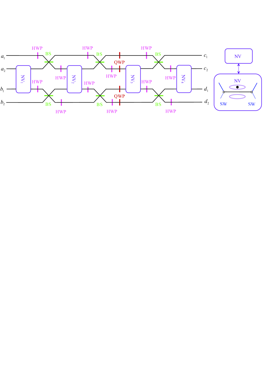
Figure 4: (Color online) Schematic diagram for the complete nondestructive analysis of two-photon polarization-spatial hyperentangled Bell states.

According to Eq.(5), after the photons pass through NV₁ and NV₂, the evolution of the system composed of the two photons and the two NV centers is shown in Table 3. One can see that the 16 polarization-spatial hyperentangled states can be divided into four groups. If both the spins of NV₁ and NV₂ are changed to be $|\varphi^{-}\rangle_{1}|\varphi^{-}\rangle_{2}$, the photon pair $ab$ is in one of the four hyperentangled Bell states $|\Phi_{1}^{\pm}\rangle_{P}|\Phi_{1}^{+}\rangle_{S}$ and $|\Phi_{2}^{\pm}\rangle_{P}|\Phi_{1}^{-}\rangle_{S}$. If both NV₁ and NV₂ stay in the initial state $|\varphi^{+}\rangle_{1}|\varphi^{+}\rangle_{2}$, the photon pair $ab$ is in one of the four hyperentangled Bell states $|\Phi_{1}^{\pm}\rangle_{P}|\Phi_{2}^{-}\rangle_{S}$ and $|\Phi_{2}^{\pm}\rangle_{P}|\Phi_{2}^{+}\rangle_{S}$. Otherwise, when NV₁ and NV₂ are in the state of $|\varphi^{-}\rangle_{1}|\varphi^{+}\rangle_{2}$ (or $|\varphi^{+}\rangle_{1}|\varphi^{-}\rangle_{2}$), the photon pair $ab$ is in one of the four hyperentangled Bell states $|\Phi_{2}^{\pm}\rangle_{P}|\Phi_{1}^{+}\rangle_{S}$ and $|\Phi_{1}^{\pm}\rangle_{P}|\Phi_{1}^{-}\rangle_{S}$ (or $|\Phi_{1}^{\pm}\rangle_{P}|\Phi_{2}^{+}\rangle_{S}$ and $|\Phi_{2}^{\pm}\rangle_{P}|\Phi_{2}^{-}\rangle_{S}$).

Table 3: The relation between the initial states and the final states of the system after the photons pass through NV₁ and NV₂.

Initial states	Final states
$|\Phi_{1}^{\pm}\rangle_{P}|\Phi_{1}^{+}\rangle_{S}|\varphi^{+}\rangle_{1}|\varphi^{+}\rangle_{2}$	$|\Phi_{1}^{\pm}\rangle_{P}|\Phi_{1}^{+}\rangle_{S}|\varphi^{-}\rangle_{1}|\varphi^{-}\rangle_{2}$
$|\Phi_{2}^{\pm}\rangle_{P}|\Phi_{1}^{+}\rangle_{S}|\varphi^{+}\rangle_{1}|\varphi^{+}\rangle_{2}$	$|\Phi_{2}^{\mp}\rangle_{P}|\Phi_{2}^{-}\rangle_{S}|\varphi^{-}\rangle_{1}|\varphi^{+}\rangle_{2}$
$|\Phi_{1}^{\pm}\rangle_{P}|\Phi_{1}^{-}\rangle_{S}|\varphi^{+}\rangle_{1}|\varphi^{+}\rangle_{2}$	$|\Phi_{1}^{\mp}\rangle_{P}|\Phi_{2}^{+}\rangle_{S}|\varphi^{-}\rangle_{1}|\varphi^{+}\rangle_{2}$
$|\Phi_{2}^{\pm}\rangle_{P}|\Phi_{1}^{-}\rangle_{S}|\varphi^{+}\rangle_{1}|\varphi^{+}\rangle_{2}$	$|\Phi_{2}^{\pm}\rangle_{P}|\Phi_{1}^{-}\rangle_{S}|\varphi^{-}\rangle_{1}|\varphi^{-}\rangle_{2}$
$|\Phi_{1}^{\pm}\rangle_{P}|\Phi_{2}^{+}\rangle_{S}|\varphi^{+}\rangle_{1}|\varphi^{+}\rangle_{2}$	$|\Phi_{1}^{\mp}\rangle_{P}|\Phi_{1}^{-}\rangle_{S}|\varphi^{+}\rangle_{1}|\varphi^{-}\rangle_{2}$
$|\Phi_{2}^{\pm}\rangle_{P}|\Phi_{2}^{+}\rangle_{S}|\varphi^{+}\rangle_{1}|\varphi^{+}\rangle_{2}$	$|\Phi_{2}^{\pm}\rangle_{P}|\Phi_{2}^{+}\rangle_{S}|\varphi^{+}\rangle_{1}|\varphi^{+}\rangle_{2}$
$|\Phi_{1}^{\pm}\rangle_{P}|\Phi_{2}^{-}\rangle_{S}|\varphi^{+}\rangle_{1}|\varphi^{+}\rangle_{2}$	$|\Phi_{1}^{\pm}\rangle_{P}|\Phi_{2}^{-}\rangle_{S}|\varphi^{+}\rangle_{1}|\varphi^{+}\rangle_{2}$
$|\Phi_{2}^{\pm}\rangle_{P}|\Phi_{2}^{-}\rangle_{S}|\varphi^{+}\rangle_{1}|\varphi^{+}\rangle_{2}$	$|\Phi_{2}^{\mp}\rangle_{P}|\Phi_{1}^{+}\rangle_{S}|\varphi^{+}\rangle_{1}|\varphi^{-}\rangle_{2}$

Subsequently, one can let the photons pass through the BS and QWP which are used to transform the phase information discrimination to parity information discrimination both for the polarization DOF and the spatial-mode DOF. According to Table 3, after the photons pass through BS and QWP, the initial hyperentangled Bell state $|\Phi_{1}^{\pm}\rangle_{P}|\Phi_{1}^{+}\rangle_{S}$ and $|\Phi_{2}^{\pm}\rangle_{P}|\Phi_{1}^{-}\rangle_{S}$ for the same group will become

$$|\Phi_{1}^{+}\rangle_{P}|\Phi_{1}^{+}\rangle_{S} \xrightarrow[]{NV_{1},NV_{2},BS,QWP} |\Phi_{1}^{+}\rangle_{P}|\Phi_{1}^{+}\rangle_{S},$$

$$|\Phi_{1}^{-}\rangle_{P}|\Phi_{1}^{+}\rangle_{S} \xrightarrow[]{NV_{1},NV_{2},BS,QWP} |\Phi_{2}^{+}\rangle_{P}|\Phi_{1}^{+}\rangle_{S},$$

$$|\Phi_{2}^{+}\rangle_{P}|\Phi_{1}^{-}\rangle_{S} \xrightarrow[]{NV_{1},NV_{2},BS,QWP} |\Phi_{1}^{-}\rangle_{P}|\Phi_{2}^{+}\rangle_{S},$$

$$|\Phi_{2}^{-}\rangle_{P}|\Phi_{1}^{-}\rangle_{S} \xrightarrow[]{NV_{1},NV_{2},BS,QWP} |\Phi_{2}^{-}\rangle_{P}|\Phi_{2}^{+}\rangle_{S}.\;\;\;\;$$ (15)

From Table 3, one can see that the final hyperentangled Bell states of two-photon systems in the same group will be changed into four different groups. By letting the photons pass through NV₃ and NV₄ which has the same syndetic connection with NV₁ and NV₂, one can distinguish those hyperentangled Bell states. The hyperentangled Bell states in the other three groups will have the same conditions. After passing through all the elements shown in Fig. 4, the final states of the two photons become those ones shown in Table 4.

Table 4: The relation between the initial hyperentangled Bell states and the final states of the two photons after passing through all the elements.

Initial states	Final states	Initial states	Final states
$|\Phi_{1}^{+}\rangle_{P}|\Phi_{1}^{+}\rangle_{S}$	$|\Phi_{1}^{+}\rangle_{P}|\Phi_{1}^{+}\rangle_{S}$	$|\Phi_{1}^{-}\rangle_{P}|\Phi_{1}^{+}\rangle_{S}$	$|\Phi_{2}^{-}\rangle_{P}|\Phi_{2}^{-}\rangle_{S}$
$|\Phi_{2}^{+}\rangle_{P}|\Phi_{1}^{+}\rangle_{S}$	$|\Phi_{2}^{-}\rangle_{P}|\Phi_{1}^{+}\rangle_{S}$	$|\Phi_{2}^{-}\rangle_{P}|\Phi_{1}^{+}\rangle_{S}$	$|\Phi_{1}^{-}\rangle_{P}|\Phi_{2}^{-}\rangle_{S}$
$|\Phi_{1}^{+}\rangle_{P}|\Phi_{1}^{-}\rangle_{S}$	$|\Phi_{2}^{+}\rangle_{P}|\Phi_{1}^{-}\rangle_{S}$	$|\Phi_{1}^{-}\rangle_{P}|\Phi_{1}^{-}\rangle_{S}$	$|\Phi_{1}^{-}\rangle_{P}|\Phi_{2}^{+}\rangle_{S}$
$|\Phi_{2}^{+}\rangle_{P}|\Phi_{1}^{-}\rangle_{S}$	$|\Phi_{1}^{+}\rangle_{P}|\Phi_{1}^{-}\rangle_{S}$	$|\Phi_{2}^{-}\rangle_{P}|\Phi_{1}^{-}\rangle_{S}$	$|\Phi_{2}^{-}\rangle_{P}|\Phi_{2}^{+}\rangle_{S}$
$|\Phi_{1}^{+}\rangle_{P}|\Phi_{2}^{+}\rangle_{S}$	$|\Phi_{2}^{+}\rangle_{P}|\Phi_{2}^{+}\rangle_{S}$	$|\Phi_{1}^{-}\rangle_{P}|\Phi_{2}^{+}\rangle_{S}$	$|\Phi_{1}^{-}\rangle_{P}|\Phi_{1}^{-}\rangle_{S}$
$|\Phi_{2}^{+}\rangle_{P}|\Phi_{2}^{+}\rangle_{S}$	$|\Phi_{1}^{+}\rangle_{P}|\Phi_{2}^{+}\rangle_{S}$	$|\Phi_{2}^{-}\rangle_{P}|\Phi_{2}^{+}\rangle_{S}$	$|\Phi_{2}^{-}\rangle_{P}|\Phi_{1}^{-}\rangle_{S}$
$|\Phi_{1}^{+}\rangle_{P}|\Phi_{2}^{-}\rangle_{S}$	$|\Phi_{1}^{+}\rangle_{P}|\Phi_{2}^{-}\rangle_{S}$	$|\Phi_{1}^{-}\rangle_{P}|\Phi_{2}^{-}\rangle_{S}$	$|\Phi_{2}^{-}\rangle_{P}|\Phi_{1}^{+}\rangle_{S}$
$|\Phi_{2}^{+}\rangle_{P}|\Phi_{2}^{-}\rangle_{S}$	$|\Phi_{2}^{+}\rangle_{P}|\Phi_{2}^{-}\rangle_{S}$	$|\Phi_{2}^{-}\rangle_{P}|\Phi_{2}^{-}\rangle_{S}$	$|\Phi_{1}^{-}\rangle_{P}|\Phi_{1}^{+}\rangle_{S}$

In this time, by using linear-optical elements, one can transform the state of the two-photon system into its initial hyperentangled Bell state. That is, one can completely distinguish the 16 hyperentangled Bell states with the measurement outcomes of the states of the four NV centers rather than using single-photon detectors to proceed destructive measurement. The relation between the initial hyperentangled Bell states and the measurement outcomes of the states of the NV centers is shown in Table 5.

Table 5: The relation between the initial hyperentangled Bell states and the measurement outcomes of the states of the NV centers.

Bell states	NV1	NV2	NV3	NV4
$|\Phi_{1}^{+}\rangle_{P}|\Phi_{1}^{+}\rangle_{S}$	$|\varphi^{-}\rangle_{1}$	$|\varphi^{-}\rangle_{2}$	$|\varphi^{-}\rangle_{3}$	$|\varphi^{-}\rangle_{4}$
$|\Phi_{1}^{-}\rangle_{P}|\Phi_{1}^{+}\rangle_{S}$	$|\varphi^{-}\rangle_{1}$	$|\varphi^{-}\rangle_{2}$	$|\varphi^{-}\rangle_{3}$	$|\varphi^{+}\rangle_{4}$
$|\Phi_{2}^{+}\rangle_{P}|\Phi_{1}^{+}\rangle_{S}$	$|\varphi^{-}\rangle_{1}$	$|\varphi^{+}\rangle_{2}$	$|\varphi^{+}\rangle_{3}$	$|\varphi^{-}\rangle_{4}$
$|\Phi_{2}^{-}\rangle_{P}|\Phi_{1}^{+}\rangle_{S}$	$|\varphi^{-}\rangle_{1}$	$|\varphi^{+}\rangle_{2}$	$|\varphi^{+}\rangle_{3}$	$|\varphi^{+}\rangle_{4}$
$|\Phi_{1}^{+}\rangle_{P}|\Phi_{1}^{-}\rangle_{S}$	$|\varphi^{-}\rangle_{1}$	$|\varphi^{+}\rangle_{2}$	$|\varphi^{-}\rangle_{3}$	$|\varphi^{-}\rangle_{4}$
$|\Phi_{1}^{-}\rangle_{P}|\Phi_{1}^{-}\rangle_{S}$	$|\varphi^{-}\rangle_{1}$	$|\varphi^{+}\rangle_{2}$	$|\varphi^{-}\rangle_{3}$	$|\varphi^{+}\rangle_{4}$
$|\Phi_{2}^{+}\rangle_{P}|\Phi_{1}^{-}\rangle_{S}$	$|\varphi^{-}\rangle_{1}$	$|\varphi^{-}\rangle_{2}$	$|\varphi^{+}\rangle_{3}$	$|\varphi^{-}\rangle_{4}$
$|\Phi_{2}^{-}\rangle_{P}|\Phi_{1}^{-}\rangle_{S}$	$|\varphi^{-}\rangle_{1}$	$|\varphi^{-}\rangle_{2}$	$|\varphi^{+}\rangle_{3}$	$|\varphi^{+}\rangle_{4}$
$|\Phi_{1}^{+}\rangle_{P}|\Phi_{2}^{+}\rangle_{S}$	$|\varphi^{+}\rangle_{1}$	$|\varphi^{-}\rangle_{2}$	$|\varphi^{+}\rangle_{3}$	$|\varphi^{+}\rangle_{4}$
$|\Phi_{1}^{-}\rangle_{P}|\Phi_{2}^{+}\rangle_{S}$	$|\varphi^{+}\rangle_{1}$	$|\varphi^{-}\rangle_{2}$	$|\varphi^{+}\rangle_{3}$	$|\varphi^{-}\rangle_{4}$
$|\Phi_{2}^{+}\rangle_{P}|\Phi_{2}^{+}\rangle_{S}$	$|\varphi^{+}\rangle_{1}$	$|\varphi^{+}\rangle_{2}$	$|\varphi^{-}\rangle_{3}$	$|\varphi^{+}\rangle_{4}$
$|\Phi_{2}^{-}\rangle_{P}|\Phi_{2}^{+}\rangle_{S}$	$|\varphi^{+}\rangle_{1}$	$|\varphi^{+}\rangle_{2}$	$|\varphi^{-}\rangle_{3}$	$|\varphi^{-}\rangle_{4}$
$|\Phi_{1}^{+}\rangle_{P}|\Phi_{2}^{-}\rangle_{S}$	$|\varphi^{+}\rangle_{1}$	$|\varphi^{+}\rangle_{2}$	$|\varphi^{+}\rangle_{3}$	$|\varphi^{+}\rangle_{4}$
$|\Phi_{1}^{-}\rangle_{P}|\Phi_{2}^{-}\rangle_{S}$	$|\varphi^{+}\rangle_{1}$	$|\varphi^{+}\rangle_{2}$	$|\varphi^{+}\rangle_{3}$	$|\varphi^{-}\rangle_{4}$
$|\Phi_{2}^{+}\rangle_{P}|\Phi_{2}^{-}\rangle_{S}$	$|\varphi^{+}\rangle_{1}$	$|\varphi^{-}\rangle_{2}$	$|\varphi^{-}\rangle_{3}$	$|\varphi^{+}\rangle_{4}$
$|\Phi_{2}^{-}\rangle_{P}|\Phi_{2}^{-}\rangle_{S}$	$|\varphi^{+}\rangle_{1}$	$|\varphi^{-}\rangle_{2}$	$|\varphi^{-}\rangle_{3}$	$|\varphi^{-}\rangle_{4}$

From the analysis above, one can see that the hyperentangled Bell states in both the polarization and the spatial-mode DOFs can be completely distinguished assisted by NV centers in diamonds confined in MTRs, and our analysis is nondestructive. Our scheme can be generalized to the complete analysis of multi-photon polarization-spatial hyperentangled GHZ states by importing more NV-center-cavity systems.

V Discussion and summary

In our schemes, the reflection coefficient of input photon pulse and the phase shift induced on the output photon play a crucial role. Under the resonant condition $\omega_{0}=\omega_{c}=\omega$, if the cavity side leakage is neglected, the fidelities of our schemes can reach 100% in the strong-coupling regime with $r(\omega)\cong 1$ and $r_{0}(\omega)\cong-1$. If the cavity leakage is taken into account, the spin-selective optical transition rules employed in our work become

$$|R\rangle|+\rangle \rightarrow r|R\rangle|+\rangle,\;\;\;\;\;\;\,|R\rangle|-\rangle\;\rightarrow\;r_{0}|R\rangle|-\rangle,$$

$$|L\rangle|+\rangle \rightarrow r_{0}|L\rangle|+\rangle,\;\;\;\;|L\rangle|-\rangle\;\rightarrow\;r|L\rangle|-\rangle.$$ (16)

Considering the practical implementation of the system, we numerically simulate the relation between the fidelities (the efficiencies) and the coupling strength g, the cavity decay rate $\kappa$, and the NV center decay rate $\gamma$. Defining the fidelity of the process for generating or completely analyzing hyperentangled states in our schemes as $F=|\langle\psi_{f}|\psi\rangle|^{2}$. Here $|\psi_{f}\rangle$ is the final state by considering the cavity side leakage and $|\psi\rangle$ denotes the final state with an ideal condition. We calculate the fidelity of our scheme for generating the hyperentangled state $|\Phi_{1}^{-}\rangle_{P}|\Phi_{1}^{-}\rangle_{S}$ and its fidelity is

$$F_{1}=\frac{(r-r_{0})^{2}(r^{2}+r_{0}^{2}+2)^{2}}{8(r^{2}+r_{0}^{2})(r^{4}+r_{0}^{4}+2)}.$$ (17)

By computations it is found, since the hyperentangled Bell states $|\Phi_{1}^{+}\rangle_{P}|\Phi_{1}^{+}\rangle_{S}$, $|\Phi_{1}^{+}\rangle_{P}|\Phi_{1}^{-}\rangle_{S}$, and $|\Phi_{1}^{-}\rangle_{P}|\Phi_{1}^{+}\rangle_{S}$ have the same parity conditions with the hyperentangled Bell state $|\Phi_{1}^{-}\rangle_{P}|\Phi_{1}^{-}\rangle_{S}$, the fidelities of our scheme for their generations are also $F_{1}$. $F_{2}$, $F_{3}$, and $F_{4}$ correspond to the fidelities for generating the hyperentangled Bell states $|\Phi_{1}^{\pm}\rangle_{P}|\Phi_{2}^{\pm}\rangle_{S}$, $|\Phi_{2}^{\pm}\rangle_{P}|\Phi_{1}^{\pm}\rangle_{S}$, and $|\Phi_{2}^{\pm}\rangle_{P}|\Phi_{2}^{\pm}\rangle_{S}$, respectively. Here

$$\begin{split}F_{2}&=\frac{(r^{2}+r_{0}^{2}+2)^{4}}{16(r^{4}+r_{0}^{4}+2)^{2}},\\ F_{3}&=\frac{(r-r_{0})^{4}}{4(r^{2}+r_{0}^{2})^{2}},\\ F_{4}&=\frac{(1-rr_{0})^{2}(r-r_{0})^{2}}{4(1+r^{2}r_{0}^{2})(r^{2}+r_{0}^{2})}.\end{split}$$ (18)

The fidelities of our HBSG scheme varies with the parameter $\text{g}/\sqrt{\kappa\gamma}$, shown in Fig. 5 (a). For our HBSG scheme, the efficiency, which is defined as the ratio of the number of the output photons to the input photons, can be written as

$$\eta_{1}=\frac{1}{2^{8}}(r^{2}+r_{0}^{2}+2)^{4}.$$ (19)

The efficiency of our HBSG scheme varies with the parameter $\text{g}/\sqrt{\kappa\gamma}$, shown in Fig. 5 (b).

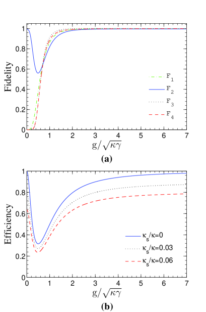
Figure 5: (Color online) (a) The fidelities of the HBSG scheme for the generation of the hyperentangled states $|\Phi_{1}^{\pm}\rangle_{P}|\Phi_{1}^{\pm}\rangle_{S}$ ($F_{1}$), $|\Phi_{1}^{\pm}\rangle_{P}|\Phi_{2}^{\pm}\rangle_{S}$ ($F_{2}$), $|\Phi_{2}^{\pm}\rangle_{P}|\Phi_{1}^{\pm}\rangle_{S}$ ($F_{3}$), and $|\Phi_{2}^{\pm}\rangle_{P}|\Phi_{2}^{\pm}\rangle_{S}$ ($F_{4}$) vs the parameter $\text{g}/\sqrt{\kappa\gamma}$ for the leakage rates $\kappa_{s}/\kappa=0.03$, respectively. (b) The efficiency of the HBSG scheme vs the parameter $\text{g}/\sqrt{\kappa\gamma}$ for different leakage rates $\kappa_{s}/\kappa$.

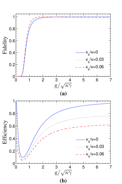
Figure 6: (Color online) (a) Fidelity of the present HBSA scheme for the hyperentangled Bell state $|\Phi_{1}^{+}\rangle_{P}|\Phi_{1}^{+}\rangle_{S}$ versus the parameter $\text{g}/\sqrt{\kappa\gamma}$ for different leakage rates $\kappa_{s}/\kappa$. (b) The efficiency of the HBSA scheme vs the parameter $\text{g}/\sqrt{\kappa\gamma}$ for different leakage rates $\kappa_{s}/\kappa$.

From Fig. 5(a), one can see that when $\text{g}/\sqrt{\kappa\gamma}=1.5$, the fidelities are $F_{1}=96.68\%$, $F_{2}=94.69\%$, $F_{3}=98.70\%$ , and $F_{1}=97.43\%$ for the leakage rates $\kappa_{s}/\kappa=0.03$, and the efficiency of our scheme is $\eta_{1}=53.96\%$ for the leakage rates $\kappa_{s}/\kappa=0.06$. When the parameter $\text{g}/\sqrt{\kappa\gamma}$ is larger than 3, the fidelities of our HBSG scheme for the hyperentangled Bell states $|\Phi_{2}^{\pm}\rangle_{P}|\Phi_{1}^{\pm}\rangle_{S}$ will be $F_{3}\approx 1$, while other fidelities are higher than $99\%$, and the efficiency of our HBSG scheme will be higher than $\eta_{1}=71.75\%$. In our protocol for generating hyperentangled GHZ states, we use three NV-center-cavity systems rather than two NV-center-cavity systems, which makes the fidelity and the efficiency of the scheme lower than those in the HBSG protocol.

The fidelity of our HBSA protocol for the hyperentangled Bell state $|\Phi_{1}^{+}\rangle_{P}|\Phi_{1}^{+}\rangle_{S}$ is given by

$$F=\frac{\varepsilon^{8}}{4(\alpha+2\beta)}.$$ (20)

Here

$$\begin{split}\alpha&=(r^{2}-r_{0}^{2})^{2}[(r-r_{0})^{2}(r^{2}+1)(r_{0}^{2}+1)\\ &\;\;\;\;+4rr_{0}(r^{2}+r_{0}^{2})],\\ \beta&=(r^{2}+r_{0}^{2})^{2}[(r^{2}+r_{0}^{2})^{2}+4r^{2}r_{0}^{2}],\\ \varepsilon&=r-r_{0}.\end{split}$$ (21)

The efficiency of our HBSA protocol is

$$\eta=\frac{1}{2^{16}}(r^{2}+r_{0}^{2}+2)^{8}.$$ (22)

Both the fidelity and efficiency of our HBSA scheme vary with the parameter $\text{g}/\sqrt{\kappa\gamma}$, shown in Fig. 6. The plots indicates that for $\text{g}/\sqrt{\kappa\gamma}\geq 0.5$ the higher fidelities and efficiencies of our HBSG scheme depend on the higher NV-cavity coupling strength. When the parameter $\text{g}/\sqrt{\kappa\gamma}$ is larger than 3, the fidelity and the efficiency will be higher than $F=99.58\%$ and $\eta=51.48\%$ for the leakage rates $\kappa_{s}/\kappa=0.06$.

The fidelity of our HBSG and HBSA schemes can be reduced a few percent because of the imperfection of electron spin population, the imperfection of the NV electron spins readout, and the imperfection of frequency-selective microwave manipulation. For $m_{s}=0$, the preparation fidelity is $99.7\pm 0.1\%$, and $99.2\pm 0.1\%$ for $m_{s}=\pm 1$ tgaebel . The average readout fidelity of the NV electron spins is $93.2\pm 0.5\%$ tgaebel . By using isotopically purified diamonds and polarizing the nitrogen nuclear spin, we can reduce the microwave manipulation imperfection. The spin decoherence may also reduce the fidelity of our schemes. In our schemes, the single photons are successively sent into the devices, the time interval $\Delta t$ between two photons should be less than the electron-spin coherence time $T$. In experimental cases, the spin relaxation time $T_{1}$ of NV centers in diamond scales from microseconds to seconds at low temperature and the dephasing time $T_{2}$ is about 2 ms in an isotopically pure diamond Neumann ; r43 . The electron-spin coherence time $T$ is $>10$ ms HBernien , which is much longer than the photon coherence time $\sim 10$ ns and the subnanosecond electron-spin manipulation control GDFuchs .

For the practical operations, the photon loss due to absorption and scatting, the mismatch between the input pulse mode and MTR, and the inefficiency of the detectors will bring ineffectiveness to our schemes. Interestingly, the photon loss will just affect the success efficiency, rather than the fidelity. The present experimental technology can generate 300000 high-quality single photons within 30 s MH . Another key ingredient of our protocols is the coupling between NV centers and MTRs. In realistic experiments, the strong coupling between the NV centers and the WGM has been demonstrated in different kinds of microcavities s33 ; nvcavity2 ; nvcavity3 ; nvcavity4 ; nvcavity5 ; nvcavity6 . The coupling strength between NV centers and the WGM can reach $\text{g}/2\pi\sim 0.3-1$GHz s33 ; nvcavity3 ; nvcavity4 ; nvcavity5 . The Q factor of the chip-based microcavity is higher than 25000. Considering the parameters $[\text{g}_{ZPL},\kappa,\gamma_{total},\gamma_{ZPL}]/2\pi=[0.30,26,0.013,0.0004]$ GHz of an NV center coupled to a microdisk nvcavity3 , we have $\text{g}\approx 3\sqrt{\kappa\gamma}$ and the fidelities of our HBSG and HBSA schemes can exceed 99%. Therefore our protocols are feasible in experiment.

Compared with previous works kerr ; HBSA2 ; HBSA3 , these two schemes relax the difficulty of their implementation in experiment as it is not difficult to generate the $\pi$ phase shift in single-sided NV-cavity systems. Moreover, single-sided NV-cavity systems have a long coherence time even at the room temperature (1.8 ms) r43 , different from quantum-dot-cavity systems. The first HBSA scheme by Sheng, Deng, and Long kerr is achieved with cross-Kerr nonlinearity. It is perfect in theory. At present, a clean cross-Kerr nonlinearity in the optical single-photon regime is still a controversial assumption with current technology kerr2 ; kerr3 . The second HBSA scheme by Ren et al. HBSA2 with single-sided quantum-dot-cavity systems requires the $\pi$ phase difference of the Faraday rotation between a hot cavity and an empty cavity, and it is not easy to acquire the phase difference with only one nonlinear interaction between a photon and a quantum dot. Compared with the work by Wang, Lu, and Long HBSA3 , our schemes do not require that the transmission for the uncoupled cavity is balanceable with the reflectance for the coupled cavity. Moreover, the coherent manipulation of the spin of a single NV center to accomplish quantum information and computation tasks at room temperature has been presented nvregister ; algorithm , which provides the basis for the current schemes.

In summary, we have proposed two efficient schemes for the deterministic generation and the complete nondestructive analysis of hyperentangled Bell states in both polarization and spatial-mode DOFs assisted by NV centers in MTRs. The HBSG protocol can also be extended to achieve the generation of multi-photon hyperentangled GHZ states efficiently. Compared with previous works kerr ; HBSA2 ; HBSA3 , our schemes relax the difficulty of their implementation in experiment. Our calculations show that the proposed schemes can work with a high fidelity and efficiency under the current experimental techniques, which may be a benefit to long-distance high-capacity quantum communication, such as quantum teleportation, quantum dense coding, and quantum superdense coding with two DOFs of photon systems.

References

- (1) J. T. Barreiro, N. K. Langford, N. A. Peters, and P. G. Kwiat, Phys. Rev. Lett. 95, 260501 (2005).
- (2) M. Barbieri, C. Cinelli, P. Mataloni, and F. De Martini, Phys. Rev. A 72, 052110 (2005).
- (3) G. Vallone, R. Ceccarelli, F. De Martini, and P. Mataloni, Phys. Rev. A 79, 030301(R) (2009).
- (4) B. C. Ren and F. G. Deng, Sci. Rep. 4, 4623 (2014).
- (5) B. C. Ren, G. Y. Wang, and F. G. Deng, Phys. Rev. A 91, 032328 (2015).
- (6) S. P. Walborn, S. Ṕadua, and C. H. Monken, Phys. Rev. A 68, 042313 (2003).
- (7) C. Schuck, G. Huber, C. Kurtsiefer, and H. Weinfurter, Phys. Rev. Lett. 96, 190501 (2006).
- (8) M. Barbieri, G. Vallone, P. Mataloni, and F. De Martini, Phys. Rev. A 75, 042317 (2007).
- (9) M. M. Wilde and D. B. Uskov, Phys. Rev. A 79, 022305 (2009).
- (10) Y. B. Sheng and F. G. Deng, Phys. Rev. A 81, 032307 (2010).
- (11) Y. B. Sheng and F. G. Deng, Phys. Rev. A 82, 044305 (2010).
- (12) F. G. Deng, Phys. Rev. A 83, 062316 (2011).
- (13) T. J. Wang, S. Y. Song, and G. L. Long, Phys. Rev. A 85, 062311 (2012).
- (14) J. T. Barreiro, T. C. Wei, and P. G. Kwiat, Nat. Phys. 4, 282 (2008).
- (15) Y. B. Sheng, F. G. Deng, and G. L. Long, Phys. Rev. A 82, 032318 (2010).
- (16) N. Pisenti, C. P. E. Gaebler, and T. W. Lynn, Phys. Rev. A 84, 022340 (2011).
- (17) B. C. Ren, H. R. Wei, M. Hua, T. Li, and F. G. Deng, Opt. Express 20, 24664 (2012).
- (18) T. J. Wang, Y. Lu, and G. L. Long, Phys. Rev. A 86, 042337 (2012).
- (19) B. C. Ren, F. F. Du, and F. G. Deng, Phys. Rev. A 88, 012302 (2013).
- (20) B. C. Ren and F. G. Deng, Laser Phys. Lett. 10, 115201 (2013).
- (21) B. C. Ren, F. F. Du, and F. G. Deng, Phys. Rev. A 90, 052309 (2014).
- (22) B. C. Ren and G. L. Long, Opt. Express 22, 6547 (2014).
- (23) X. H. Li and S. Ghose, Laser Phys. Lett. 11, 125201 (2014).
- (24) X. H. Li and S. Ghose, Opt. Express 23, 3550 (2015).
- (25) F. Jelezko, T. Gaebel, I. Popa, A. Gruber, and J. Wrachtrup, Phys. Rev. Lett. 92, 076401 (2004).
- (26) G. Davies and M. F. Hamer, Proc. R. Soc. A 348, 285 (1976).
- (27) A. Gruber, A. Dräbenstedt, C. Tietz, L. Fleury, J. Wrachtrup, and C. von Borczyskowski, Science 276, 2012 (1997).
- (28) M. V. Gurudev Dutt, L. Childress, L. Jiang, E. Togan, J. Maze, F. Jelezko, A. S. Zibrov, P. R. Hemmer, and M. D. Lukin, Science 316, 1312 (2007).
- (29) T. van der sar, Z. H. Wang, M. S. Blok, H. Bernien, T. H. Taminiau, D. M. Toyli, D. A. Lidar, D. D. Awschalom, R. Hanson, and V. V. Dobrovitski, Nature (London) 484, 82 (2012).
- (30) A. Beveratos, R. Brouri, T. Gacoin, J. P. Poizat, and P. Grangier, Phys. Rev. A 64, 061802(R) (2001).
- (31) C. Kurtsiefer, S. Mayer, P. Zarda, and H.Weinfurter, Phys. Rev. Lett. 85, 290 (2000).
- (32) L. Childress, M. V. G. Dutt, J. M. Taylor,A. S. Zibrov, F. Jelezko, J. Wrachtrup, P. R. Hemmer, andM. D. Lukin, Science 314, 281 (2006).
- (33) P. Neumann, N. Mizuochi, F. Rempp, P. Hemmer, H. Watanable, S. Yamasaki, V. Jacques, T. Gaebel, F. Jelezko, and J. Wrachtrup, Science 320, 1326 (2008).
- (34) E. Togan, Y. Chu, A. S. Trifonov, L. Jiang, J. Maze, L. Childress, M. V. G. Dutt, A. S. Srensen, P. R. Hemmer, A. S. Zibrov, and M. D. Lukin, Nature (London) 466, 730 (2010).
- (35) K. Xia, G. K. Brennen, D. Ellinas, and J. Twamley, Opt. Express 20, 27198 (2012).
- (36) W. L. Yang, Z. Q. Yin, Z. Y. Xu, M. Feng, and C. H. Oh, Phys. Rev. A 84, 043849 (2011).
- (37) Y. S. Park, A. K. Cook, and H. Wang, Nano Lett. 6, 2075 (2006).
- (38) B. Dayan, A. S. Parkins, T. Aoki, E. P. Ostby, K. I. Vahala, and H. J. Kimble, Science 319, 1062 (2008).øø
- (39) A. Young, C. Y. Hu, L. Marseglia, J. P. Harrison, J. L. O’Brien, and J. G. Rarity, New J. Phys. 11, 013007 (2009).
- (40) B. B. Buckley, G. D. Fuchs, L. C. Bassett, and D. D. Awschalom, Science 330, 1212 (2010).
- (41) W. L. Wang, Z. Y. Xu, M. Feng, and J. F. Du, New J. Phys. 12, 113039 (2010).
- (42) Q. Chen, W. L. Wang, M. Feng, and J. F. Du, Phys. Rev. A 83, 054305 (2011).
- (43) H. R. Wei and F. G. Deng, Phys. Rev. A 88, 042323 (2013).
- (44) C. Wang, Y. Zhang, G. S. Jin, and R. Zhang, J. Opt. Soc. Am. B 29, 3349 (2013).
- (45) S. M. Spillane, T. J. Kippenberg, K. J. Vahala, K. W. Goh, E. Wilcut, and H. J. Kimble, Phys. Rev. A 71, 013817 (2005).
- (46) Y. Louyer, D. Meschede, and A. Rauschenbeutel, Phys. Rev. A 72, 031801(R) (2005).
- (47) A. Lenef and S. C. Rand, Phys. Rev. B 53, 13441 (1995).
- (48) T. Gaebel, M. Domhan, I. Popa, C. Wittmann, P. Neumann,F. Jelezko, J. R. Rabeau, N. Stavrias, A. D. Greentree, S. Prawer, J. Meijer, J. Twamley, P. R. Hemmer, and J. Wrachtrup, Nat. Phys. 2, 408 (2006).
- (49) L. Robledo, L. Childress, H. Bernien, B. Hensen, P. F. A. Alkemade, and R. Hanson, Nature (London) 477, 574 (2011).
- (50) G. Balasubramanian, P. Neumann, D. Twitchen, M. Markham, R. Kolesov, N. Mizuochi, J. Isoya, J. Achard, J. Beck, J. Tissler, V. Jacques, P. R. Hemmer, F. Jelezko, and J. Wrachtrup, Nat. Mater. 8, 383 (2009).
- (51) H. Bernien, B. Hensen, W. Pfaff, G. Koolstra, M. S. Blok, L. Robledo, T. H. Taminiau, M. Markham, D. J. Twitchen, L. Childress, and R. Hanson, Nature (London) 497, 86 (2013).
- (52) G. D. Fuchs, V. V. Dobrovitski, D. M. Toyli, F. J. Here- mans, and D. D. Awschalom, Science 326, 1520 (2009).
- (53) M. Hijlkema, B. Weber, H. P. Specht, S. C. Webster, A. Kuhn, and G. Rempe, Nat. Phys. 3, 253 (2007).
- (54) M. W. McCutcheon, M. Lončar, Opt. Express 16, 19136 (2008).
- (55) P. E. Barclay, K. M. Fu, C. Santori, R. G. Beausoleil, App. Phys. Lett. 95, 191115 (2009).
- (56) P. E. Barclay, C. Santori, K. M. Fu, R. G. Beausoleil, and O. Painter1, Opt. Express 17, 8081 (2009).
- (57) M. Larsson, K. N. Dinyari, H. Wang, Nano Lett. 9 1447 (2009).
- (58) D. Englund, B. Shields, K. Rivoire, F. Hatami, J. Vuckovic, H. Park, M. D. Lukin, Nano Lett. 10, 3922 (2010).
- (59) J. H. Shapiro, Phys. Rev. A 73, 062305 (2006).
- (60) J. Gea-Banacloche, Phys. Rev. A 81, 043823 (2010).
- (61) P. Neumann, R. Kolesov, B. Naydenov, J. Beck, F. Rempp, M. Steiner, V. Jacques, G. Balasubramanian, M. L. Markham, D. J. Twitchen, S. Pezzagna, J. Meijer, J. Twamley, F. Jelezko, and J. Wrachtrup, Nat. Phys. 6, 249 (2010).
- (62) F. Shi, X. Rong, N. Xu, Y. Wang, J. Wu, B. Chong, X. Peng, J. Kniepert, R. S. Schoenfeld, W. Harneit, M. Feng, and J. F. Du, Phys. Rev. Lett. 105, 040504 (2010).