We give a brief survey of thermodynamic metrics, in particular the Hessian of the entropy function, and how they apply to black hole thermodynamics. We then provide a detailed discussion of the Gibbs surface of Kerr black holes. In particular we analyze its global properties, and extend it to take the entropy of the inner horizon into account. A brief discussion of Kerr-Newman black holes is included.

1. Introduction

This Special Issue concerns geometry in thermodynamics, and there is a branch of thermodynamics arising out of geometry—namely black hole thermodynamics. The fundamental relations that describe black holes have a number of special features. Many of them can be traced back to the fact that—unlike the thermodynamic systems that dominate textbooks on thermodynamics [1, 2, 3]—black holes cannot spontaneously divide themselves into subsystems. Mathematically, their entropies are not extensive functions, and hence the usual arguments connecting stability to the concavity of the entropy function do not apply.

Here we will be concerned with the information geometry of black holes. We take the rather restrictive view that this means that we are to study the (negative of) the Hessian of their entropy functions, interpreted as a metric tensor. This geometry is also known as the Ruppeiner geometry [4], and its physical relevance is well established for a wide class of thermodynamic systems such as fluid and spin systems, but not really—despite a considerable amount of work—for black holes. There is a dream however, which is that it may have something to say about the obvious question: what properties must a function have if it is to serve as an entropy function for black holes? The equilibrium states form a Gibbs surface, and the question is how we can recognize that a Gibbs surface with a given geometry and global shape is a black hole Gibbs surface? We have no answer to offer, but at least we can look for clues.

We will begin our paper with a brief review of the foundations of Ruppeiner’s geometry (sections 2 and 3). This is followed by a brief comment on entropic substances (section 4). We will then bring up the points where the discussion must be changed for non-extensive systems (section 5). In section 6 we give an in-depth discussion of the Ruppeiner geometry of the Kerr family of black holes, with special emphasis on the global nature of the Gibbs surface. In section 7 we partially extend this discussion to the Kerr-Newman family. The new results are summarized in section 8. In the end we will not arrive at a definite physical interpretation of the Ruppeiner geometry of black holes, but we hope that we have made a contribution towards this goal. The Ruppeiner geometry does encode information about the second variation of the entropy function for some of the most intriguing thermodynamic systems known.

2. Ruppeiner geometry

The Ruppeiner metric is defined on the Gibbs surface of a thermodyamic system using nothing but the fundamental relation $S=S(X)$, where $S$ is the entropy and $X^{i}$ are the remaining extensive variables of the system including its energy [4]. The metric tensor is simply the negative of the Hessian matrix,

$$g_{ij}\equiv-\frac{\partial^{2}S}{\partial X^{i}\partial X^{j}}\equiv-S_{,ij}\ .$$ (1)

(Note the notation for partial derivatives introduced in the second step. We will use it freely from now on.) A slightly older definition uses the Hessian of the energy as a function of the extensive variables including the entropy. This is called the Weinhold metric [5]. These definitions are mathematically natural if there is an affine structure defined on the space coordinatized by the arguments of the functions. The metric preserves its form under affine coordinate transformations. (The analogy to Kähler metrics will strike readers familiar with the latter. In that case it is a complex rather than an affine structure that enables us to define the metric in terms of a potential without bringing in any non-zero Christoffel symbols.) A theory of Hessian metrics has been developed within mathematical statistics [6]. In the simplest case one considers the (the negative of) the Hessian of the Shannon entropy. The resulting metric is known as the Fisher-Rao metric, and has an interpretation in terms of the distinguishability of nearby distributions under a large number of samplings. In this case there are clear connections to thermodynamic geometry [7].

The notation of thermodynamics was not designed to do differential geometry. In particular functions are given names depending on the physical interpretation of the values they take, rather than on their mathematical form. Let us denote the extensive variables, including the energy $U$, as $X^{i}=(U,N^{a})$. We may pass to the energy representation, where the extensive variables are $Y^{i}=(S,N^{a})$. Intensive variables ${\mu}_{i}$, such as temperature, pressure and chemical potential, are usually defined through

$$dU={\mu}_{i}dY^{i}=TdS+{\mu}_{a}dN^{a}\ ,$$ (2)

while the intensive variables in the entropy representation have no agreed names. The fundamental relation takes one of the forms $U=U(S,N^{a})$ or $S=S(U,N^{a})$. The Weinhold metric is

$$ds^{2}_{W}=U_{,ij}dY^{i}\otimes_{S}dY^{j}=d{\mu}_{j}\otimes_{S}dY^{j}=dT\otimes_{S}dS+d{\mu}_{a}\otimes_{S}dN^{a}\ ,$$ (3)

and the Ruppeiner metric is

$$ds^{2}=-S_{,ij}dX^{i}\otimes_{S}dX^{j}=-d\left(\frac{1}{T}\right)\otimes_{S}dU+d\left(\frac{{\mu}_{a}}{T}\right)\otimes_{S}dN^{a}\ .$$ (4)

These two metrics are conformally related [8],

$$ds^{2}=\frac{1}{T}(dT\otimes_{S}dS+d{\mu}_{a}\otimes_{S}dN^{a})=\frac{1}{T}ds^{2}_{W}\ .$$ (5)

As long as the temperature $T$ is positive both metrics are positive definite whenever $S$ is a concave function. Once these metrics have been written down in their defining representations one can perform coordinate changes freely. If the state space is two dimensional they can be diagonalized by using $T$ as a coordinate.

Extensive systems have the property that (for $\lambda>0$)

$$\lambda S(X)=S(\lambda X)\ ,$$ (6)

and similarly for the energy function. Euler’s theorem on homogeneous functions can then be used together with the first law to derive the Gibbs-Duhem relation:

$$U=Y^{i}\mu_{i}\hskip 14.22636pt\Rightarrow\hskip 14.22636ptdU=\mu_{i}dY^{i}+Y^{i}d\mu_{i}\hskip 14.22636pt\Rightarrow\hskip 14.22636ptY^{i}d{\mu}_{i}=0\ .$$ (7)

Then the thermodynamic metrics will be degenerate. Indeed we see that

$$d{\mu}_{i}=g^{W}_{ij}dY^{j}\hskip 14.22636pt\Rightarrow\hskip 14.22636ptY^{i}g^{W}_{ij}dY^{j}=0\hskip 14.22636pt\Rightarrow\hskip 14.22636ptY^{i}g^{W}_{ij}=0\ .$$ (8)

Hence every metric conformal to the Weinhold metric has a null eigenvector. In order to obtain a positive definite metric we must keep one extensive variable fixed. This is also required by the physical setting of thermodynamic fluctuation theory, which is usually assumed to concern a (sub-)system at fixed volume but fluctuating energy.

3. Physical interpretation and the role of curvature

The Ruppeiner geodetic distance can be interpreted as follows. Choose a path on the Gibbs surface. Divide it into $N$ steps, where $N$ is large. Start the system at one of the chosen points, and change its environment so that it equilibrates to the next point on the path. To fix ideas, think of changing the state of a cup of coffee by moving it through a succession of $N$ rooms at different temperatures. An elegant argument [9] then shows that the total entropy change of the “universe”—the rooms and the coffee, in our example—in the limit of large $N$, is bounded from below by

$$\Delta S^{\rm U}\geq\frac{D^{2}}{2N}\ ,$$ (9)

where $D$ is the Ruppeiner length of the path. It follows that the lowest possible bound on $\Delta S^{\rm U}$ is obtained when the system is driven along a geodetic path. The Weinhold geodetic distance has an interpretation along similar lines [9]. This result is of interest in finite time thermodynamics [10], and in computer simulations of small systems [11].

Ruppeiner originally introduced his metric in the context of thermodynamic fluctuation theory. We recall that this was initiated by Einstein, who inverted Boltzmann’s formula $S=\ln{\Omega}$ (in the equiprobable case). The entropy assumes a maximum at equilibrium, and we can expand to second order in the fluctuations (assumed to be small). This leads to a probability distribution for the fluctuations which, using the properties of Gaussian integrals, is shown to have the form [1]

$$p(X)=Ce^{S(X)}\approx Ce^{S(X_{0})+\frac{1}{2}\frac{\partial^{2}S}{\partial X^{i}\partial X^{j}}{\Big{|}}_{X_{0}}\Delta X^{i}\Delta X^{j}}=\frac{\sqrt{\det{g}}}{(2{\pi})^{\frac{N}{2}}}e^{-\frac{1}{2}g_{ij}\Delta X^{i}\Delta X^{j}}\ ,$$ (10)

where $g_{ij}$ is the Ruppeiner metric (and $N$ is the number of variables). All functions are evaluated at equilibrium and both sides of the equation transform like a density, as it should be. In the normalization we assumed positive definiteness of the metric, which is equivalent to the concavity of the entropy function. In a typical application one extensive variable is kept fixed, and provides a scale. Thus, if the volume of the fluctuating subsystem is fixed, we should work with

$$S=Vs(u,n)$$ (11)

where $u=U/V$ etc. At least in the small, the Ruppeiner distance now acquires a meaning in terms of distinguishability against the background of the fluctuations.

The Riemann curvature scalar plays a major role in Ruppeiner’s theory [4, 12]. In the first place it determines the accuracy of the approximation made in eq. (10). This is related to one of the main geometric roles of the curvature scalar, to determine the growth in volume of a small ball with its radius. In any curved space the volume of a ball of geodesic radius $r$ is related to the volume of a ball of radius $r$ in flat space through

$$\frac{\mbox{Vol}(\circ)}{\mbox{Vol}_{0}(\circ)}=1-\frac{r^{2}R(0)}{6(d+2)}+\dots\ ,$$ (12)

where $\mbox{Vol}_{0}$ is the volume of a ball in flat space, $d$ is the dimension, and $R(0)$ is the curvature scalar at the centre of the ball. This universal formula holds to lowest order in the radius $r$. The sign of the curvature scalar therefore carries important information. Finally the Riemann tensor governs the way geodesics deviate from each other.

Ruppeiner argues that attractive forces between the microscopic constituents give positive curvature, repulsive forces give negative curvature. The sign of the curvature also distinguishes between the Bose and Fermi ideal gases [13]. This picture is supported by numerous studies of model systems, especially fluid systems with two dimensional Gibbs surfaces [14, 15], and in particular their behaviour at phase transitions. The Ruppeiner and the Weinhold geometry of the ideal gas are flat, equally so if the volume or the particle number is kept fixed.

4. Entropic substances

A small comment on when the Ruppeiner metric is flat may be useful. The ideal gas is the prime example of substance in which the only forces acting on the constituents are constraint forces. Other examples exist, notably—to a good approximation—rubber. On the macroscopic level such substances obey caloric equations of state of the form $U=U(T)$. So, consider an inflated rubber balloon at room temperature. One might think that its radius is obtained by minimizing its energy subject to some constraints, but this is clearly wrong since its thermodynamic energy is unaffected by changes in the volume of the ideal gas or in the tension of the rubber. What does determine the radius of the balloon is that it maximizes its entropy. For this reason such materials go under the name entropic substances [16].

Is it perhaps so that entropic substances always have flat thermodynamical metrics? For the Ruppeiner metric on a two dimensional Gibbs surface the answer is “yes”. To avoid confusion concerning the notation, let us denote the energy by $x$, the other variables in the fundamental relation by $y$, and the entropy function whose Hessian we are interested in by $\psi=\psi(x,y)$. The material will be entropic if its temperature $1/\psi_{,x}$ is a function of the energy $x$ only, that is to say if there exists a function $f$ such that

$$\psi_{,x}=f(x)\ .$$ (13)

It follows immediately (using overdots to denote derivatives) that

$$\psi_{,xx}=\dot{f}\hskip 28.45274pt\psi_{,xxx}=\ddot{f}\hskip 28.45274pt\psi_{,xy}=\psi_{,xxy}=\psi_{,xxy}=0\ .$$ (14)

The Riemann tensor of a Hessian metric involves second and third derivatives of $\psi$ only, and in two dimensions these conditions are enough to ensure that the Riemann tensor vanishes (and also that the Ruppeiner metric is diagonal in these coordinates). But this does not have to be so in higher dimensions, so the general answer to our question is “no”.

The Weinhold metric can still be curved, also for two dimensional systems. To see this we denote the entropy by $x$, the other variable in the fundamental relation by $y$, and the energy function whose Hessian we are interested in by $\psi=\psi(x,y)$. The material will be entropic if there exists a function $f$ such that

$$\psi_{,x}=f(\psi)\ .$$ (15)

After some calculation one finds, for the curvature scalar of a two dimensional system, that

$$R_{W}=\frac{1}{2g^{2}}\dot{f}\ddot{f}\left[f^{2}\psi_{,yy}^{2}-2f\dot{f}\psi_{,yy}\psi_{,y}^{2}+\dot{f}^{2}\psi_{,y}^{4}\right]\ .$$ (16)

This does not vanish in general, although it does vanish when $\ddot{f}=0$, so that $T$ and $U$ are linearly related. This is the case for the ideal gas.

There is more to a geometry than its local curvature. Globally the Gibbs surface of the ideal gas when equipped with the Ruppeiner metric is an infinite flat plane if $S=S(U,V)$. If $S=S(U,N)$ it is an infinite covering of the flat plane with one point (at $N=0$) removed [17]. We are not aware of a physical interpretation of this difference (although the latter result can be understood from general considerations [18]).

5. The transition to black holes

We now come to black holes. They are equilibrium states of Einstein’s relativity theory, and can be regarded as thermodynamic systems with the total mass $M$ of the spacetimes containing them serving as the energy function and one quarter of the area of their event horizon serving as their entropy. This truly remarkable result makes dimensional sense only because of the introduction of Planck’s constant $\hbar$ (which is seemingly foreign to the theory) into the equations [19, 20, 21].

Black hole entropy functions depend on mechanically conserved control parameters such as mass $M$, angular momentum $J$, and electric charge $Q$, so an affine structure is there. However, these entropy functions are not concave (unless the black hole is confined to a cavity, as is effectively the case if we add a negative cosmological constant), and the Ruppeiner metric is no longer positive definite. Many of the preceding arguments have to be rethought in this new context. The density of states grows fast with energy, which means that the canonical ensemble misbehaves [21]. Moreover, specific heats can be negative, with no immediate consequences for stability. Negative specific heats do in fact occur in self-gravitating gases in the Newtonian regime too, as is well known among astronomers [22]. The analogy should perhaps not be pushed too far, but like black holes self-gravitating gases cannot spontaneously divide themselves into parts, and they are therefore non-extensive systems. Early arguments about phase transitions caused by diverging specific heats [23] are contradicted by analyses based on Poincaré’s linear series method [24, 25]. For the Kerr black holes they show that that no instability is present in the microcanonical ensemble, given that the Schwarzschild black hole is stable (except for an intriguing hint of instability in the extreme limit [25]). The Ruppeiner metric does not come into the question of the dynamical stability of a black hole at all, since this is a question about variations at constant ADM mass, not within a family of black holes described by a Gibbs surface. It does have consequences for black brane solutions however [26].

The role of the curvature scalar is somewhat changed in Lorentzian spaces since there do not exist round balls there. Their role is taken by causal diamonds, consisting of the intersection of a past and a future lightcone whose apices are connected by a timelike geodesic. The volume of a small causal diamond is [27, 28] (choosing our conventions so that de Sitter space has $R>0$)

$$\frac{\mbox{Vol}(\diamond)}{\mbox{Vol}_{0}(\diamond)}=1+\frac{d}{24(d+1)}\left(R_{ab}+\frac{R}{d+2}g_{ab}\right)t^{a}t^{b}+\dots\ ,$$ (17)

where the right hand side is evaluated at the midpoint of the geodetic segment and $t^{a}$ is its tangent vector, normalized so that

$$g_{ab}(0)t^{a}t^{b}=-\tau^{2}\ .$$ (18)

A directional dependence has entered the formula. In two dimensions, where $R_{ab}=Rg_{ab}/2$, it enters only at the next order:

$$\frac{\mbox{Vol}(\diamond)_{2}}{\mbox{Vol}_{0}(\diamond)_{2}}=1-\frac{R}{48}\tau^{2}-\frac{1}{5760}\left(4g_{ab}R^{2}-g_{ab}\nabla^{2}R+3\nabla_{a}\nabla_{b}R\right)t^{a}t^{b}\tau^{2}+\dots\ .$$ (19)

It should also be noted that negative curvature, say, will cause timelike geodesics to converge and spacelike geodesics to diverge.

The thermodynamic geometry of black holes was first discussed (briefly) by Page [29], then by Ferrara et al. [30], and later by many others. In fact the literature is by now large and varied, as can be gleaned from the reference lists in some recent papers [15, 31, 32]. As an example of a direction that we will not look into here, let us mention the idea that the non-equivalence of ensembles in the black hole case means that the Hessian of other thermodynamic potentials, such as the free energy, should be studied; see ref. [33] and references therein.

For our present purposes it must be mentioned that the scale symmetry of Einstein-Maxwell equations, with the cosmological constant set to zero but with the spacetime dimension $d\geq 4$ kept arbitrary, implies that the entropy of any black hole is a generalized homogeneous function. With $J$ being the angular momentum and $Q$ the electric charge there holds

$$\lambda^{d-2}S(M,Q,J)=S(\lambda^{d-3}M,\lambda^{d-3}Q,\lambda^{d-2}J)\ .$$ (20)

It follows that the thermodynamic metrics will admit a homothetic Killing vector field, and also that there is a close relative of the Gibbs-Duhem relation. The intensive variables are the Hawking temperature $T$, the electric potential $\Phi$ at the horizon, and the angular velocity $\Omega$ of the horizon. The Hawking temperature is simply related to a geometrical property of the event horizon known as its surface gravity. From eq. (20) one may deduce the Smarr formula [34]

$$(d-3)M=(d-2)ST+(d-3)Q\Phi+(d-2)J\Omega\ .$$ (21)

For the Kerr and Reissner-Nordström families the implication is that there exist functions $f$ of one variable such that

$$S=M^{c_{1}}f(M^{c_{2}}X)$$ (22)

(where $X$ denotes either $J$ or $Q$), with exponents that are easily calculable. But every entropy function of the form (22) leads to a flat Ruppeiner metric if $c_{2}=-1$, and a flat Weinhold metric if $c_{1}+c_{2}=0$ [18]. With no further assumptions about the form of the function $f$ it then follows that the Ruppeiner metric of the Reissner-Nordström families, and the Weinhold metric of the Kerr families, are both flat.

In the next two sections we will go a bit beyond these known results, especially as concerns the global geometry of the state spaces.

6. Kerr black holes

Given the interest in higher dimensional versions of physics, and the various matter fields suggested by all sorts of theories, there is a large and varied supply of black hole families to discuss. However, we will concentrate on the Kerr family, for the obvious reason that this is the only family that can make a solid case for actual existence. It is believed that many Kerr black holes do exist in the Milky Way, including a large one at its centre [35].

We need to know that the event horizon of a Kerr black hole with mass $M$ and angular momentum $J$ has area

$$A_{+}=8\pi M^{2}\left(1+\sqrt{1-J^{2}/M^{4}}\right)\ .$$ (23)

The event horizon exists only if the angular momentum is bounded by the inequality $-M^{2}\leq J\leq M^{2}$ (in suitable units), which in everyday terms is a very strong constraint. The exact solution also has an inner horizon with area

$$A_{-}=8\pi M^{2}\left(1-\sqrt{1-J^{2}/M^{4}}\right)\ .$$ (24)

If $J/M^{2}=\pm 1$ the two horizons coincide and we have an extreme black hole with vanishing surface gravity (that is, vanishing Hawking temperature). Since the inner horizon will play an important role below we should perhaps say that there is no reason to believe that the spinning black hole at the centre of the Milky Way has an inner horizon. The sense in which that black hole is likely to be modelled by the Kerr solution is bound up with asymptotics, just as the equilibrium states and quasi-static processes of textbook thermodynamics are useful shorthands for a more complicated reality.

We take the view that the inner horizon is an important feature of the equilibrium state. Its thermodynamics has already received some attention in the literature [36, 37]. Consequently we have two distinct entropy functions to study, namely

$$S_{\pm}=S_{\pm}(M,J)=\frac{k}{4}A_{\pm}=2M^{2}\left(1\pm\sqrt{1-J^{2}/M^{4}}\right)\ .$$ (25)

(Following Davies we have set Boltzmann’s constant $k=1/\pi$ [23].) There will also be two different Hawking temperatures

$$T_{\pm}=\pm\frac{1}{4M}\frac{\sqrt{1-J^{2}/M^{4}}}{1\pm\sqrt{1-J^{2}/M^{4}}}\ .$$ (26)

They both vanish in the extreme limit. Otherwise $T_{+}$ is positive and $T_{-}$ is negative.

If we invert the entropy function to obtain the mass $M$ as a function of entropy and angular momentum we find the same functional form in both cases,

$$M=\sqrt{\frac{S_{\pm}}{4}+\frac{J^{2}}{S_{\pm}}}\ .$$ (27)

Consequently we will obtain the same expression for its Hessian, the Weinhold metric, in both cases—only the range of the coordinates will differ.

The expressions for the Weinhold and Ruppeiner metrics in their defining coordinates are not very illuminating [38]. Changing to the dimensionless coordinate

$$a=\frac{J}{M^{2}}\ ,\hskip 14.22636pt-1\leq a\leq 1\ ,$$ (28)

and using our expression for $T_{\pm}$, we obtain for the two Ruppeiner metrics

$$ds^{2}_{\pm}=\frac{1}{T_{\pm}}\left[-\frac{dM^{2}}{M}+\frac{M}{2}\frac{da^{2}}{(1-a^{2})(1\pm\sqrt{1-a^{2}})}\right]\ .$$ (29)

The expression within brackets gives the Weinhold metric. To bring the latter to manifestly flat form we perform a sequence of coordinate transformations, viz.

$$a=\sin{2\beta}\ ,\hskip 14.22636pt\cosh{2\alpha}=\frac{1}{\cos{\beta}}\ ,$$ (30)

$$t=2\sqrt{M}\cosh{\alpha}\ ,\hskip 14.22636ptx=2\sqrt{M}\sinh{\alpha}\ .$$ (31)

The result is that

$$ds^{2}_{\pm}=\frac{1}{T_{\pm}}\left[-dt^{2}+dx^{2}\right]\ .$$ (32)

We must now consider the coordinate ranges.

In the calculation we made use of the equation $\sqrt{1-a^{2}}=\cos{2\beta}$, so it is clear that the range $-\pi/4\leq\beta\leq\pi/4$ must be used for the Ruppeiner metric $ds^{2}_{+}$ associated to the outer horizon. Its Gibbs surface is a timelike wedge, with a locally flat Minkowski metric for its Weinhold metric. The wedge is bounded by

$$-\sqrt{\frac{\sqrt{2}-1}{\sqrt{2}+1}}\leq\frac{x}{t}\leq\sqrt{\frac{\sqrt{2}-1}{\sqrt{2}+1}}=\tan{\frac{\pi}{8}}\ .$$ (33)

Its opening angle is $45^{\circ}$. The Ruppeiner metric itself is not defined on the edge of the wedge, since the conformal factor diverges there. However, the Weinhold metric can evidently be analytically extended. By increasing the coordinate range to $-\pi/2\leq\beta\leq\pi/2$ we include also the Gibbs surface corresponding to the inner horizon. The combined Gibbs surface is isometric to the future null cone of Minkowski space, as far as its Weinhold metric is concerned. We find this satisfying.

Using the Minkowski space coordinates we can now give unifying expressions for the thermodynamic functions. The mass and the entropy are

$$M=\frac{t^{2}-x^{2}}{4}$$ (34)

$$S=2M^{2}(1\pm\sqrt{1-a^{2}})=M^{2}(1+\cos{2\beta})=\frac{(t^{2}-x^{2})^{4}}{4(t^{2}+x^{2})^{2}}\ .$$ (35)

Both of them vanish on the light cone (while they remain finite on the edge of the wedge, where the extreme black holes sit). The Hawking temperatures $T_{\pm}$ are unified to

$$T=\frac{(t^{2}-x^{2}-2tx)(t^{2}-x^{2}+2tx)}{2(t^{2}-x^{2})^{3}}\ .$$ (36)

Its variation over the Gibbs surface is shown in Fig. 2.

The state space volume, as measured by the Ruppeiner metric, is strongly concentrated to the neighbourhood of the extreme black holes. The Ruppeiner curvature scalar is

$$R=-\frac{4(t^{4}+10t^{2}x^{2}+x^{4})}{(t^{2}-x^{2})^{2}(t^{4}-6t^{2}x^{2}+x^{4})}\ .$$ (37)

It diverges at the edge of the wedge and on the null cone, as seen in Fig. 2.

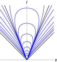
Figure 1: Contour curves of equal Hawking temperature $T$. The Hawking temperature vanishes at the edge of the wedge that corresponds to the outer horizon, is negative outside, and diverges on the null cone.

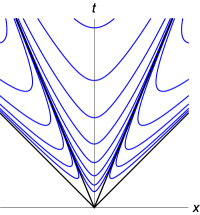
Figure 2: Contour curves of equal Ruppeiner scalar curvature $R$. It is negative inside the wedge, positive outside, and diverges both at the edge of the wedge and on the null cone.

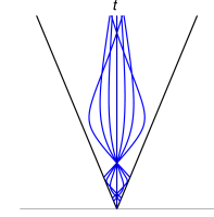
Figure 3: Timelike geodesics inside the wedge.

Figure 4: Spacelike and null geode- sics inside the wedge.

To get a firm grasp of the curved geometry we observe, in Figs. 3-4, that timelike geodesics (inside the wedge) tend to converge, and in fact they oscillate back and forth around the $t$-axis (corresponding to the spinless Schwarzschild black holes). We are unable to suggest a physical interpretation of these geodesics. It might be interesting to investigate how some physical processes that may occur close to equilibrium appear when drawn as curves in this picture. An example of such a process, which has the double advantage of being determined by the parameters of the black hole itself and of having a simple analytical form, is accretion of matter from the innermost stable circular orbit of an accretion disk. This was described by Bardeen [39], who showed that an initially Schwarzschild black hole of mass $M_{i}$ will spin up according to the formula

$$a=\sqrt{\frac{2}{3}}\frac{M_{i}}{M}\left[4-\left(\frac{18M_{i}^{2}}{M^{2}}-2\right)^{1/2}\right]\ ,\hskip 22.76219ptM_{i}\leq M\leq\sqrt{6}M_{i}\ .$$ (38)

However, the resulting curve starts out spacelike and ends up timelike, so it seems fair to say that it is totally insensitive of the Ruppeiner geometry.

The absence of explicit experimental protocols for how to drive a black hole along specified curves in state space is deplorable. One obvious target would be the Penrose process, briefly alluded to in Fig. 5, but we are not aware of any suitable analytic formulas.

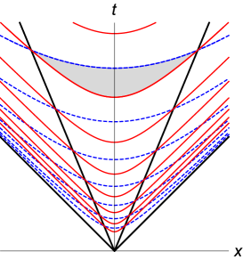
Figure 5: Contour curves for entropy and mass (dashed). By moving inside the grey area, from near the edge of the wedge (large $a$) towards the centre, one is able to decrease the mass (extract energy) even though the area of the event horizon (the entropy) increases [40], as it must according to Einstein’s theory.

7. The Kerr-Newman family of black holes

We have stressed that the scale invariance of Einstein’s equations (with a vanishing cosmological constant) dictates the form of the entropy function (22), and it is this form of the entropy function that dictates the wedge shaped state space associated with the outer horizon [18]. For Kerr black holes in five dimensions the picture is qualitatively the same as that pertaining to four dimensions, but in six or more dimensions black holes of the Myers-Perry variety do not have extreme limits, and the wedge shaped state space associated with the outer (only) horizon then fills the entire future null cone [41, 42]. Another example where the wedge fills the entire null cone is that of Einstein-Maxwell-dilaton black holes, which again lack an extreme limit [43]. In both cases the thermodynamic null cone is given by the equation $S=0$, although for the Reissner-Nordström black holes it is the Ruppeiner metric that is the flat one.

The Einstein-Maxwell equations contains a three parameter family of black hole equilibrium states. The fundamental relation of these Kerr-Newman black holes is

$$S=2M^{2}-Q^{2}+2M^{2}\sqrt{1-\frac{Q^{2}}{M^{2}}-\frac{J^{2}}{M^{4}}}\$$ (39)

where $J$ is the angular momentum and $Q$ the electric charge of the black hole. What is the geometry and global shape of this Gibbs surface?

It is convenient to rewrite the fundamental relation in terms of dimensionless variables,

$$S=M^{2}f(q,a)\ ,\hskip 34.1433ptq=\frac{Q}{M}\ ,\hskip 28.45274pta=\frac{J}{M^{2}}\ .$$ (40)

The form of the function $f$ can be read out from eq. (39). The Ruppeiner metric is a complicated affair in its defining coordinates. Transforming to the coordinates $(\mu,q,a)$, where

$$M=e^{\mu}\ ,$$ (41)

it takes the reasonably attractive form

$$ds^{2}=e^{2\mu}\left[2(af_{,a}-f)d\mu^{2}-2f_{,q}d\mu dq-f_{,qq}dq^{2}-2f_{,qa}dqda-f_{,aa}da^{2}\right]\ .$$ (42)

There is a homothetic Killing vector field

$$\xi=M\partial_{M}=\partial_{\mu}\ ,\hskip 22.76219pt{\cal L}_{\xi}g=2g\ .$$ (43)

The boundary of state space occurs for extreme black holes (or when the event horizon becomes a degenerate Killing horizon), namely when

$$T=0\hskip 14.22636pt\Leftrightarrow\hskip 14.22636pt1=q^{2}+a^{2}\ .$$ (44)

The Ruppeiner curvature scalar, and the Ricci tensor in an orthonormal frame, are everywhere finite in the interior and diverge at the boundary. The actual expressions are complicated [44, 45].

Thus the Gibbs surface of the Kerr-Newman black holes assumes the shape of a positive cone, with the rays defined by the homothetic Killing vector field. This is an interesting shape for a state space to assume. The elegance is marred by the fact that the homothetic Killing vector field fails to be surface forming. This follows from a simple calculation verifying that

$$\xi_{[a}\nabla_{b}\xi_{c]}\neq 0\ .$$ (45)

Other proposals for thermodynamic metrics exist [46], and do not suffer from this seeming defect [47], but we have not considered them. The homothetic Killing vector field is timelike everywhere within the cone corresponding to the outer horizon (but this is not so for the homothetic Killing vector field in the Weinhold geometry).

The question whether the inner horizon can be used to extend the Gibbs surface beyond the surface of the cone corresponding to the outer horizon is non-trivial. In the Kerr case we relied on the flat Weinhold metric to perform this extension. In the Kerr-Newman case the Weinhold curvature scalar remains finite throughout the interior of the cone, but it diverges at the rays $q=\pm 1$ corresponding to extreme Reissner-Nordström black holes. Outside the cone it diverges along a two-dimensional surface. None of the two homothetic Killing vector fields would be timelike everywhere inside the null cone. It is not clear to us how this can be handled (if indeed it can be handled).

8. Discussion

It seemed appropriate, on this occasion, to review the various uses that thermodynamic metrics have been put to—restricting ourselves throughout to the Hessian metrics proposed by Weinhold and Ruppeiner. Some of our results are (we think) new. We raised and answered the question whether all entropic substances have flat thermodynamic metrics. The answer is “no”. We analytically extended the thermodynamic geometry of the Kerr black holes to include the entire future null cone of a two dimensional Lorerentzian space. This was achieved by the inclusion of the entropy function for the inner horizon, using the Weinhold metric in a key role. We went on to clarify in what sense the state space of the Kerr-Newman black holes is a cone. It has been known for some time that the scale invariance of Einstein’s equations implies that wedge shaped state spaces in the interior of the thermodynamic null cone arise for all sorts of black hole families, but these analyses were concerned with the entropy function defined by the outer horizon only.

There are many things we would like to know, but don’t. First of all we have not analyzed what restrictions on the function $f$, in entropy functions of the form given in eq. (22), make the extension of the wedge to include the entire light cone possible. It does not seem to be straightforward in the Reissner-Nordström case, once we insist that the extension be related to the entropy function of the inner horizon. Moreover, and crucially, a cosmological constant introduces a new scale and complicates matters. This also is known [38], but not in anything like the detail that we would like to see. The entropy function will still be approximately a generalized homogeneous function close to the origin, so some features of our analysis will survive.

We have certainly not reached the point where we can tell from the shape of the Gibbs surface that we are dealing with black hole thermodynamics.

References

- [1] L. D. Landau and E. M. Lifshitz: Statistical Physics, Pergamon, London 1959.
- [2] H. B. Callen: Thermodynamics and an Introduction to Thermostatistics, Springer, New York 1985.
- [3] F. Weinhold: Classical and Geometrical Theory of Chemical and Phase Thermodynamics, Wiley, Hoboken 2009
- [4] G. Ruppeiner, Riemannian geometry in thermodynamic fluctuation theory, Rev. Mod. Phys. 67 (1995) 605; Rev. Mod. Phys. 68 (313(E)).
- [5] F. Weinhold, Thermodynamics and geometry, Physics Today, March 1976.
- [6] S. Amari: Differential Geometric Methods in Statistics, Springer 1985.
- [7] D. J. Brody and D. W. Hook, Information geometry in vapour-liquid equilibrium, J. Phys. A42 (2008) 023001.
- [8] P. Salamon, J. Nulton, and E. Ihrig, On the relation between entropy and energy versions of thermodynamic length, J. Chem. Phys. 80 (1984) 436.
- [9] P. Salamon, J. D. Nulton, and R. S. Berry, Length in statistical thermodynamics, J. Chem. Phys. 82 (1985) 2433.
- [10] B. Andresen, P. Salamon, and R. S. Berry, Thermodynamics in finite time, Physics Today, September 1984.
- [11] G. Cooks, Measuring thermodynamic length, Phys. Rev. Lett. 99 (2007) 100602.
- [12] G. Ruppeiner, Thermodynamic curvature measures interactions, Am. J. Phys. 78 (2010) 1170.
- [13] H. Janyszek and R. Mrugała, Riemannian geometry and stability of ideal quantum gases, J. Phys. A23 (1990) 467.
- [14] D. A. Johnston, W. Janke, and R. Kenna, Information geometry, one, two, three (and four), Acta Phys. Pol. B34 (2003) 4923.
- [15] G. Ruppeiner, Thermodynamic curvature and black holes, in Breaking of Supersymmetry and Extended Supergravity, Springer Proc. in Phys. 153 (2014) 179.
- [16] I. Müller and P. Strehlow: Rubber and Rubber Balloons, Springer, Berlin 2004.
- [17] J. D. Nulton and P. Salamon, Geometry of the ideal gas, Phys. Rev. A31 (1985) 2520.
- [18] J. E. Åman, I. Bengtsson, and N. Pidokrajt, Flat information geometries in black hole thermodynamics, Gen. Rel. Grav. 38 (2006) 1305.
- [19] J. M. Bardeen, B. Carter, and S. W. Hawking, The four laws of black hole mechanics, Commun. Math. Phys. 31 (1973) 161.
- [20] J. Bekenstein, Black holes and entropy, Phys. Rev. D7 (1973) 2333.
- [21] S. W. Hawking, Black holes and thermodynamics, Phys. Rev. D13 (1976) 191.
- [22] D. Lynden-Bell, Negative specific heat in astronomy, physics and chemistry, Physica A123 (1999) 293.
- [23] P. C. W. Davies, The thermodynamic theory of black holes, Proc. Roy. Soc. A353 (1977) 499.
- [24] J. Katz, I. Okamoto, and O. Kaburaki, Thermodynamic stability of pure black holes, Class. Quant. Grav. 10 (1993) 1323.
- [25] G. Arcioni and E. Lozano-Tellechea, Stability and critical phenomena of black holes and black rings, Phys. Rev. D72 (2005) 104021.
- [26] S. Hollands and R. M Wald, Stability of black holes and black branes, Commun. Math. Phys. 321 (2013) 629.
- [27] J. Myrheim, Statistical geometry, CERN preprint TH.25 38-CERN (1978).
- [28] G. W. Gibbons and S. N. Solodukhin, The geometry of small causal diamonds, Phys. Lett. B649 (2007) 317; erratum arXiv:hep-th/0703098.
- [29] D. N. Page, Thermodynamic paradoxes, Physics Today, January 1977.
- [30] S. Ferrara, G. W. Gibbons, and R. Kallosh, Black holes and critical points in moduli space, Nucl. Phys. B500 (1997) 75.
- [31] A. J. M. Medved, A commentary on Ruppeiner metrics for black holes, Mod. Phys. Lett. A23 (2008) 2149.
- [32] B. P. Dolan, The intrinsic curvature of thermodynamic potentials for black holes with critical points, eprint arXiv:1504.0295.
- [33] A. Bravetti and F. Nettel, Thermodynamic curvature and ensemble non-equivalence, Phys. Rev. D90 (2014) 044064.
- [34] L. Smarr, Mass formula for Kerr black holes, Phys. Rev. Lett. 30 (1973) 71.
- [35] D. L. Wiltshire, M. Visser, and S. J. Scott (eds.): The Kerr Spacetime. Rotating Black Holes in General Relativity, CUP, Cambridge 2009.
- [36] A. Curir, Spin entropy of a rotating black hole, Nuovo Cim. 51B (1979) 262.
- [37] I. Okamoto and O. Kaburaki, The ’inner-horizon thermodynamics’ of the Kerr black holes, Mon. Not. R. astr. Soc. 255 (1992) 539.
- [38] J. E. Åman, I. Bengtsson, and N. Pidokrajt, Geometry of black hole thermodynamics, Gen. Rel. Grav. 35 (2003) 1733.
- [39] J. M Bardeen, Kerr metric black holes, Nature 226 (1970) 64.
- [40] D. Christodoulou, Reversible and irreversible transformations in black-hole physics, Phys. Rev. Lett. 25 (1970) 1596.
- [41] J. E. Åman and N. Pidokrajt, Geometry of higher-dimensional black hole thermodynamics, Phys. Rev. D73 (2006) 024017.
- [42] J. E. Åman and N. Pidokrajt, On explicit thermodynamic functions and extremal limits of Myers-Perry black holes, Eur. Phys. J. C73 (2013) 2601.
- [43] J. E. Åman, N. Pidokrajt, and J. Ward, On geometro-thermodynamics of dilaton black holes, EAS Pub. Ser. 30 (2008) 279.
- [44] B. Mirza and M. Zamaninasab, Ruppeiner geometry of RN black holes: flat or curved?, J. High Energy Phys. 6 (2007) 059.
- [45] G. Ruppeiner, Thermodynamic curvature and phase transitions in Kerr-Newman black holes, Phys. Rev. D78 (2008) 024016.
- [46] J. L. Alvarez, H. Quevedo, and A. Sanchez, Unified geometric description of black hole thermodynamics, Phys. Rev. D77 (2008) 084004.
- [47] E. Anderson, Kerr-Newman black hole thermodynamical state space: blockwise coordinates, Gen. Rel. Grav. 45 (2013) 2545.