A uniqueness result on the decompositions of a bi-homogeneous polynomial

Abstract.

In the first part of this paper we give a precise description of all the minimal decompositions of any bi-homogeneous polynomial $p$ (i.e. a partially symmetric tensor of $S^{d_{1}}V_{1}\otimes S^{d_{2}}V_{2}$ where $V_{1},V_{2}$ are two complex, finite dimensional vector spaces) if its rank with respect to the Segre-Veronese variety $S_{d_{1},d_{2}}(V_{1},V_{2})$ is at most $\min\{d_{1},d_{2}\}$. Such a polynomial may not have a unique minimal decomposition as $p=\sum_{i=1}^{r}\lambda_{i}p_{i}$ with $p_{i}\in S_{d_{1},d_{2}}(V_{1},V_{2})$ and $\lambda_{i}$ coefficients, but we can show that there exist unique $p_{1},\ldots,p_{r^{\prime}}$, $p_{1}^{\prime},\ldots,p_{r^{\prime\prime}}^{\prime}\in S_{d_{1},d_{2}}(V_{1},V_{2})$, two unique linear forms $l\in V_{1}^{*}$, $l^{\prime}\in V_{2}^{*}$, and two unique bivariate polynomials $q\in S^{d_{2}}V_{2}^{*}$ and $q^{\prime}\in S^{d_{1}}V_{1}^{*}$ such that either $p=\sum_{i=1}^{r^{\prime}}\lambda_{i}p_{i}+l^{d_{1}}q$ or $p=\sum_{i=1}^{r^{\prime\prime}}\lambda^{\prime}_{i}p_{i}^{\prime}+l^{\prime d_{2}}q^{\prime}$, ($\lambda_{i},\lambda^{\prime}_{i}$ being appropriate coefficients).

In the second part of the paper we focus on the tangential variety of the Segre-Veronese varieties. We compute the rank of their tensors (that is valid also in the case of Segre-Veronese of more factors) and we describe the structure of the decompositions of the elements in the tangential variety of the two-factors Segre-Veronese varieties.

Introduction

Let $V_{1},V_{2}$ be vector spaces of dimension $n_{i}+1$ for $i=1,2$ defined over an algebraically closed vector field $K$ of characteristic zero. The space $S^{d_{1}}V_{1}\otimes S^{d_{2}}V_{2}$ is the space of partially symmetric tensors of type $T_{1}\otimes T_{2}$ where $T_{i}\in S^{d_{i}}V_{i}$ is a completely symmetric tensor of order $d_{i}$ for $i=1,2$. Since $S^{d_{i}}V_{i}$ can be interpreted also as the space of homogeneous polynomials of degree $d_{i}$ in the set of variables $\{x_{i,0},\ldots,x_{i,k}\}$ defined over $K$, i.e. $S^{d_{i}}V_{i}^{*}\simeq K[x_{i,0},\ldots,x_{i,n_{i}}]_{d_{i}}$ for $i=1,2$, then the space $S^{d_{1}}V_{1}^{*}\otimes S^{d_{2}}V_{2}^{*}$ represents also bi-homogeneous polynomials of type $p=p_{1}p_{2}$ with $p_{i}\in K[x_{i,0},\ldots,x_{i,n_{i}}]_{d_{i}}$ for $i=1,2$.

The embedding of $\mathbb{P}(V_{1})\times\mathbb{P}(V_{2})$ into $\mathbb{P}(S^{d_{1}}V_{1}\otimes S^{d_{2}}V_{2})$ induced by the complete linear system $|\mathcal{O}_{\mathbb{P}(V_{1})\times\mathbb{P}(V_{2})}(d_{1},d_{2})|$ is the so called two factors Segre-Veronese variety and it is denoted by $S_{d_{1},d_{2}}(V_{1},V_{2})$. It can be viewed as the variety parameterizing projective classes of partially symmetric tensors that can be written as:

$$T=v_{1}^{\otimes d_{1}}\otimes v_{2}^{\otimes d_{2}}$$

with $v_{i}\in V_{i}$ for $i=1,2$. In terms of multi-homogeneous polynomials, $S_{d_{1},d_{2}}(V_{1},V_{2})$ can be interpreted as the variety parameterizing projective classes of bi-homogeneous polynomial of type

$$p=l_{1}^{d_{1}}l_{2}^{d_{2}}$$

where $l_{i}$ are linear forms in $S^{1}V_{i}^{*}\simeq K[x_{i,0},\ldots,x_{i,n_{i}}]_{1}$, $i=1,2$.

We will say that an element of the Segre-Veronese variety has rank $1$. The minimum integer $r$ such that a bi-homogeneous polynomial $p$ (a two factors partially symmetric tensor $T$) can be written as a linear combination of $r$ rank 1 bi-homogeneous polynomials (two factors partially symmetric tensors) is called the rank of $p$ and it is denoted by $r(p)$ (or $r(T)$ respectively). By an abuse of notation we will say that such an $r$ is also the rank of the projective class $[p]$ of $p$ (the projective class $[T]$ of $T$ respectively).

From now on we will indicate with $p$ both the bi-homogeneous polynomial and the corresponding partially symmetric tensor.

One of the main problems of the fieldwork on a minimal decomposition of a polynomial or of a tensor is the knowledge of its possible uniqueness or identifiability. Many branches of pure and applied mathematics are nowadays very active in this field, see for example [12, 1, 17, 16, 2, 9, 11, 19, 20, 21, 8, 7].

Suppose that $\mathcal{W}\subset\mathbb{P}^{r}$ is a non-degenerate reduced and irreducible projective variety and that a point $[p]\in\mathcal{W}$ lies on a $r$-secant space $H\simeq\mathbb{P}^{r-1}$ to $\mathcal{W}$ and not on any $\mathbb{P}^{r-2}$ that is $(r-1)$-secant. A very general fact on the uniqueness of minimal decomposition is the following one.

Definition 0.1.

Let $\rho^{\prime}(\mathcal{W})$ be the maximal integer $t$ such that any subset of $\mathcal{W}$ with cardinality $t$ is linearly independent.

General fact: If $2r\leq\rho^{\prime}(\mathcal{W})$, then $H$ is the only one $r$-secant space to $\mathcal{W}$ containing $[p]$ (crf. [15, Theorem 1.18]).

This fact, translated in terms of bi-homogeneous polynomials (or two factors partially symmetric tensors), means that if $p\in S^{d_{1}}V_{1}^{*}\otimes S^{d_{2}}V_{2}^{*}$ is such that

$$r(p)\leq\rho^{\prime}(S_{d_{1},d_{2}}(V_{1},V_{2}))$$

then $p$ has a unique minimal decomposition as

(1) $$p=\sum_{i}^{r}\lambda_{i}l_{i}^{d_{1}}l_{i}^{\prime d_{2}}$$

with $l_{i}\in V_{1}^{*},l^{\prime}_{i}\in V_{2}^{*}$, $\lambda_{i}\in K$, $i=1,\ldots,r$.
In terms of two factors partially symmetric tensors it means that

(2) $$p=\sum_{i=1}^{r}\lambda_{i}v_{i}^{\otimes d_{1}}\otimes v_{i}^{\prime\otimes d_{2}}$$

with $v_{i}\in V_{1},v_{i}^{\prime}\in V_{2}$, $\lambda_{i}\in K$, $i=1,\ldots,r$.

If $X$ is the Segre-Veronese variety of $k$ factors (i.e. $X=S_{d_{1},\ldots,d_{k}}(V_{1},\ldots,V_{k})$ is the embedding of $\mathbb{P}(V_{1})\times\cdots\times\mathbb{P}(V_{k})$ into $\mathbb{P}(S^{d_{1}}V_{1}\otimes\cdots\otimes S^{d_{k}}V_{k})$ induced by the complete linear system $|\mathcal{O}_{\mathbb{P}(V_{1})\times\cdots\times\mathbb{P}(V_{k})}(d_{1},\ldots,d_{k})|$), then we have that $\rho^{\prime}(X)=1+\min_{1\leq i\leq k}\{d_{i}\}$ (in absence of a standard reference for this quite obvious fact, for sake of completeness, we give the proof in Lemma 1.13 at the end of Section 1). Unfortunately this integer is quite low, but in the case of bi-homogeneous polynomials where

$$\rho^{\prime}(S_{d_{1},d_{2}}(V_{1},V_{2}))=1+\min\{d_{1},d_{2}\},$$

we may get a stronger uniqueness result (roughly by a factor $2$). In the main result of this paper that is Theorem 1.4 we show the exact structure of the unique minimal decomposition of a bi-homogeneous polynomial $p$ (order 2 partially symmetric tensor) with $r(p)\leq\rho^{\prime}(S_{d_{1},d_{2}}(V_{1},V_{2}))$. Moreover we can also prove that the same decomposition’s structure holds for a bigger class of bi-homogeneous polynomials, namely it holds for any $p\in S^{d_{1}}V_{1}^{*}\otimes S^{d_{2}}V_{2}$ with $2r({p})\leq 1+d_{1}+d_{2}$ and $|d_{1}-d_{2}|\leq 2$ (the case where $p$ is actually a homogeneous polynomial in only one set of variables is slightly different, we treat it separately, cfr. (iii) in Theorem 1.4, and we don’t describe it here in the Introduction). In this last case the decomposition as sum of elements in $S_{d_{1},d_{2}}(V_{1},V_{2})$ won’t be unique anymore, but we have another kind of uniqueness.
In order to facilitate the reading of the first two items of Theorem 1.4, let us be more explicit here. In both cases, i.e. if either $2r({p})\leq 1+d_{1}+d_{2}$ and $|d_{1}-d_{2}|\leq 2$ (except if $p$ is a homogeneous polynomial where the situation will be anyway explicitly described in (iii) of Theorem 1.4 and Remark 1.11) or if $r({p})\leq\min\{d_{1},d_{2}\}$ we show that there exist:

• Unique $p_{1},\ldots,p_{r^{\prime}},p_{1}^{\prime},\ldots,p_{r^{\prime\prime}}^{\prime}\in S_{d_{1},d_{2}}(V_{1},V_{2})$,

• Two unique linear forms $l\in V_{1}^{*}$, $l^{\prime}\in V_{2}^{*}$,

• Two unique spaces of bi-variate linear forms $W_{1}^{*}=K[m,n]_{1}\subset V_{1}^{*}$, $W_{2}^{*}=K[m^{\prime},n^{\prime}]_{1}\subset V_{2}^{*}$, with $m,n\in V_{1}^{*},m^{\prime},n^{\prime}\in V_{2}^{*}$ linear forms, and

• The following bivariate polynomials $q_{1},\ldots,q_{s}\in S^{d_{2}}W_{2}^{*}$, $q_{1}^{\prime},\ldots,q_{s^{\prime}}^{\prime}\in S^{d_{1}}W_{1}^{*}$

such that either

$$p=\sum_{i=1}^{r^{\prime}}\lambda_{i}p_{i}+l^{d_{1}}\cdot\left(\sum_{i=1}^{s}\gamma_{i}q_{i}\right),$$

or

$$p=\sum_{i=1}^{r^{\prime\prime}}\lambda^{\prime}_{i}p_{i}^{\prime}+\left(\sum_{i=1}^{s^{\prime}}\gamma^{\prime}_{i}q^{\prime}_{i}\right)\cdot l^{\prime d_{2}}$$

with $\lambda_{i},\lambda^{\prime}_{j},\gamma_{k},\gamma^{\prime}_{h}\in K$.
If we are in case in which the bi-homogeneous polynomial $p$ has at least two different decompositions (i.e. the $q_{i}$’s and the $q_{i}^{\prime}$’s are not unique), then $2r({p})>\min\{d_{1},d_{2}\}$ and there are infinitely many choices for $\{q_{1},\ldots,q_{s}\}\subset S^{d_{2}}W_{2}^{*}$ and infinitely many choices for $\{q_{1}^{\prime},\ldots,q_{s^{\prime}}^{\prime}\}\subset S^{d_{1}}W_{1}^{*}$, but the forms $q=\sum_{i=1}^{s}\gamma_{i}q_{i}\in S^{d_{2}}W_{2}^{*}$ and $q^{\prime}=\sum_{i=1}^{s^{\prime}}\gamma_{i}q_{i}^{\prime}\in S^{d_{1}}W_{1}^{*}$ will be unique (more precisely, there are infinitely many choices if and only if there are at least two choices and this is the case if and only if either $s>\lfloor(d_{1}+1)/2\rfloor$ or $s>\lfloor(d_{2}+2)/2\rfloor$). Therefore, in this last case, we will have that either

$$p=\sum_{i=1}^{r^{\prime}}\lambda_{i}p_{i}+l^{d_{1}}q,$$

or

$$p=\sum_{i=1}^{r^{\prime\prime}}\lambda^{\prime}_{i}p_{i}^{\prime}+q^{\prime}l^{\prime d_{2}}$$

and all the forms appearing in the decomposition will be unique. In this sense we can speak of “ unique decomposition ” of the bi-homogeneous polynomial $p$. Knowing either $q$ or $q^{\prime}$, the finding of $\{q_{1},\ldots,q_{s}\}\subset S^{d_{2}}W_{2}^{*}$ or of $\{q_{1}^{\prime},\ldots,q_{s^{\prime}}^{\prime}\}\subset S^{d_{1}}W_{1}^{*}$ is assured by the classical study of bivariate polynomials with rank bigger than their border rank due to the celebrated Sylvester’s theorem (cfr. [3], [18], [22, §1.3], [23] and [10, 13] for algorithmic computation of the solutions).

We can rephrase all this in terms of two-factors partially-symmetric tensors. Let $p\in S^{d_{1}}V_{1}\otimes S^{d_{2}}V_{2}$. If either $2r({p})\leq 1+d_{1}+d_{2}$ and $|d_{1}-d_{2}|\leq 2$ (except again if $p$ is a completely symmetric tensor where the situation will be anyway explicitly described in (iii) of Theorem 1.4 and Remark 1.11) or if $r({p})\leq\min\{d_{1},d_{2}\}$ we show that there exist:

• Unique vectors $v_{j,1},\ldots,v_{j,r^{\prime}},v_{j,1}^{\prime},\ldots,v_{j,r^{\prime\prime}}^{\prime}\in V_{j}$, for $j=1,2$,

• Two unique vectors $u\in V_{1}$, $u^{\prime}\in V_{2}$,

• Two unique lines $W_{1}\subset V_{1}$, $W_{2}\subset V_{2}$ and

• The following vectors $w_{1},\ldots,w_{s}\in W_{2}$, $w_{1}^{\prime},\ldots,w_{s^{\prime}}^{\prime}\in W_{1}$

such that either

$$p=\sum_{i=1}^{r^{\prime}}\lambda_{i}v_{1,i}^{\otimes d_{1}}\otimes v_{2,i}^{\otimes d_{2}}+u^{\otimes d_{1}}\otimes\left(\sum_{i=1}^{s}\gamma_{i}w_{i}^{\otimes d_{2}}\right),$$

or

$$p=\sum_{i=1}^{r^{\prime\prime}}\lambda^{\prime}_{i}v_{1,i}^{\prime\otimes d_{1}}\otimes v_{2,i}^{\prime\otimes d_{2}}+\left(\sum_{i=1}^{s^{\prime}}\gamma^{\prime}_{i}w_{i}^{\otimes d_{1}}\right)\otimes u^{\prime\otimes d_{2}}$$

with $\lambda_{i},\lambda^{\prime}_{j},\gamma_{k},\gamma^{\prime}_{h}\in K$.
If $p$ is a two-factors partially-symmetric tensor without unique decomposition (i.e. $w_{i}$’s and $w_{i}^{\prime}$’s are not unique), then $r({p})>\min\{d_{1},d_{2}\}$, then there are infinitely many choices for $\{w_{1},\ldots,w_{s}\}\subset W_{2}$ and infinitely many choices for $\{w_{1}^{\prime},\ldots,w_{s^{\prime}}^{\prime}\}\subset W_{1}$, but the tensors $w=\sum_{i=1}^{s}\gamma_{i}w_{i}^{\otimes d_{2}}\in S^{d_{2}}W_{2}$ and $w^{\prime}=\sum_{i=1}^{s^{\prime}}\gamma_{i}w_{i}^{\prime\otimes d_{1}}\in S^{d_{1}}W_{1}$ will be unique (more precisely, there are infinitely many choices if and only if there are at least two choices and this is the case if and only if either $s>\lfloor(d_{1}+1)/2\rfloor$ or $s>\lfloor(d_{2}+2)/2\rfloor$). Therefore, in this last case, we will have that either

$$p=\sum_{i=1}^{r^{\prime}}\lambda_{i}v_{1,i}^{\otimes d_{1}}\otimes v_{2,i}^{\otimes d_{2}}+u^{\otimes d_{1}}\otimes w,$$

or

$$p=\sum_{i=1}^{r^{\prime\prime}}\lambda^{\prime}_{i}v_{1,i}^{\prime\otimes d_{1}}\otimes v_{2,i}^{\prime\otimes d_{2}}+w^{\prime}\otimes u^{\prime\otimes d_{2}}$$

and all the tensors appearing in the decomposition will be unique. In this sense we can speak of “ unique decomposition ” of the tensor $p$. As above, knowing either $w$ or $w^{\prime}$, the finding of $\{w_{1},\ldots,w_{s}\}\subset W_{2}^{*}$ or of $\{w_{1}^{\prime},\ldots,w_{s^{\prime}}^{\prime}\}\subset W_{1}^{*}$ is assured by the classical study of bivariate polynomials with rank bigger than their border rank due to the celebrated Sylvester’s theorem (cfr. [3], [18], [22, §1.3], [23] and [10, 13] for algorithmic computation of the solutions).

It will be remarkable that the numbers $r^{\prime}$ and $r^{\prime\prime}$ and the subspaces $W_{1}\subset V_{1}$ and $W_{2}\subset V_{2}$ will depend only on $[p]$ and not on the decomposition (this will be the content of Proposition 1.6).

In the second part of the paper we focus on tangential variety to Segre-Veronese variety.

In Section 2 we will consider the Segre-Veronese variety $S_{d_{1},\ldots,d_{k}}(V_{1},\ldots,V_{k})$ of any number of factors.
We will indicate with $r_{d_{1},\ldots,d_{k}}(p)$ the minimum integer $r$ such that the projective class of the multi-homogeneous polynomial $p\in S^{d_{1}}V_{1}^{*}\otimes\cdots\otimes S^{d_{k}}V_{k}^{*}$ (the partially symmetric tensor $p\in S^{d_{1}}V_{1}\otimes\cdots\otimes S^{d_{k}}V_{k}$) can be written as a sum of elements in $S_{d_{1},\ldots,d_{k}}(V_{1},\ldots,V_{k})$. Since in this case there won’t be any risk of confusion on the number of factors of the Segre-Veronese variety, by an abuse of notation we will call $r_{d_{1},\ldots,d_{k}}(p)$ the rank of $p$.

In Section 2 we show that the rank of any point $[p]$ in the tangential variety of the Segre-Veronese of $k$-factors $\tau(S_{d_{1},\ldots,d_{k}}(V_{1},\ldots,V_{k}))$ is $\sum_{i=1}^{h}d_{i}$ if $V_{1}^{*}=K[x_{1,0},\ldots,x_{1,n_{1}}]_{1}$, $\ldots,$ $V_{h}^{*}=K[x_{h,0},\ldots,x_{h,n_{h}}]_{1}$ are the minimum sets of variables to which the multi-homogeneous polynomial $p$ actually depends on, $h\leq k$. In terms of partially symmetric tensors this means that the tensor depends actually on $h\leq k$ factors: $p\in S^{d_{1}}V_{1}\otimes\cdots\otimes S^{d_{h}}V_{h}\subset S^{d_{1}}V_{1}\otimes\cdots\otimes S^{d_{k}}V_{k}$.

Finally in Section 3 we show that, if we keep focusing on the two-factors Segre-Veronese variety, then we are able to use all the mechanism that we have developed in Section 1 to describe the structure of the decompositions of the elements in $\tau(S_{d_{1},d_{2}}(V_{1},V_{2}))$. In Theorem 3.4 we show that the decomposition of an element $[p]\in\tau(S_{d_{1},d_{2}}(V_{1},V_{2}))$ is always of type

$$p=l_{1}^{d_{1}}\cdot\left(\sum_{i=1}^{r_{1}}\lambda_{i}m_{i}^{d_{2}}\right)+\left(\sum_{i=1}^{r_{2}}\gamma_{i}n^{d_{1}}_{i}\right)\cdot l_{2}^{d_{2}}$$

with $r_{1}+r_{2}=r(p)$, $m_{i}\in K[l_{1},l_{1}^{\prime}]_{1}$, $n_{i}\in K[l_{2},l_{2}^{\prime}]$, binary linear forms ($l_{i},l_{i}^{\prime}$ are linear forms in $V_{i}^{*}$, $i=1,2$) and $\lambda_{j},\gamma_{k}\in K$. This decomposition has the obvious two “ exceptions ” of either $r_{1}=0$ or $r_{2}=0$ where only one of the two addenda appears in the decomposition.

This can be translated in terms of partially symmetric tensors by saying that any element of the tangential variety of the two factors Segre-Veronese can be decomposed as

$$p=v_{1}^{\otimes d_{1}}\otimes\left(\sum_{i=1}^{r_{1}}\lambda_{i}w_{i}^{\otimes d_{2}}\right)+\left(\sum_{i=1}^{r_{2}}\gamma_{i}u_{i}^{\otimes d_{1}}\right)\otimes v_{2}^{\otimes d_{2}}$$

where $w_{i}\in\langle v_{1},v_{1}^{\prime}\rangle$ and $u_{i}\in\langle v_{2},v_{2}^{\prime}\rangle$ with $v_{i},v_{i}^{\prime}\in V_{i}$ for $i=1,2$, and $\lambda_{j},\gamma_{k}\in K$, except if either $r_{1}=0$ or $r_{2}=0$ and then only one of the two addenda appears in the decomposition.

1. A unique decomposition theorem for Segre-Veronese of two factors

Now denote by

$$\nu_{d_{1},d_{2}}:\mathbb{P}(V_{1})\times\mathbb{P}(V_{2})\to\mathbb{P}(S^{d_{1}}V_{1}\otimes S^{d_{2}}V_{2})$$

the Segre-Veronese embedding of bi-degree $(d_{1},d_{2})$ induced by the complete linear system $|\cal{O}_{\mathbb{P}(V_{1})\times\mathbb{P}(V_{2})}(d_{1},d_{2})|$.

Since $\dim V_{i}=n_{i}+1$, all along this paper we will use indistinctly the notation $\mathbb{P}(V_{i})=\mathbb{P}^{n_{i}}$.

Definition 1.1.

For any $p\in S^{d_{1}}V_{1}\otimes S^{d_{2}}V_{2}$ let $\mathcal{S}({p})$ denote the set of all finite sets of points $S\subset\mathbb{P}^{n_{1}}\times\mathbb{P}^{n_{2}}$ evincing $r({p})$, i.e. such that $[p]\in\langle\nu_{d_{1},d_{2}}(S)\rangle$ and $\sharp(S)=r({p})$.

Definition 1.2.

Let $[p_{2}]\in\mathbb{P}^{n_{2}}$ and $L$ be a line of $\mathbb{P}^{n_{1}}$, we call $L\times[p_{2}]\subset\mathbb{P}^{n_{1}}\times\mathbb{P}^{n_{2}}$ an $\alpha$-line; while if we take $[p_{1}]\in\mathbb{P}^{n_{1}}$ and $L$ being a line of $\mathbb{P}^{n_{2}}$, we call $[p_{1}]\times L\subset\mathbb{P}^{n_{1}}\times\mathbb{P}^{n_{2}}$ a $\beta$-line. Moreover we will call $\mathbb{P}^{n_{1}}\times[p_{2}]$ an $\alpha$-slice, and $[p_{1}]\times\mathbb{P}^{n_{2}}$ a $\beta$-slice.

Notation 1.3.

In the sequel, the symbol “ $\sqcup$  ” indicates the disjoint union.

Theorem 1.4 (The decomposition theorem).

Let $p\in S^{d_{1}}V_{1}\otimes S^{d_{2}}V_{2}$ be a bi-homogeneous polynomial of rank $r(p)$ such that

1. either $2r({p})\leq 1+d_{1}+d_{2}$ and $|d_{1}-d_{2}|\leq 2$,

2. or $r({p})\leq\min\{d_{1},d_{2}\}$.

Assume that there exist two different sets of points $S,A$ evincing $r(p)$, i.e. $S,A\in\mathcal{S}({p})$. Then one of the following cases occurs:

1. There are:

   • an integer $b$ with $2\leq b\leq(d_{2}+2)/2$ and $r({p})\geq d_{2}+2-b$,

   • a $\beta$-line $\mathcal{B}:=[p_{1}]\times L\subset\mathbb{P}^{n_{1}}\times\mathbb{P}^{n_{2}}$,

   • and a set of points $E\subset\mathbb{P}^{n_{1}}\times\mathbb{P}^{n_{2}}$

   such that $\sharp(E)=r({p})+b-d_{2}-2$, $E\cap\mathcal{B}=\emptyset$, $S=E\sqcup\left(S\cap\mathcal{B}\right)$ and $A=E\sqcup\left(A\cap\mathcal{B}\right)$ (see Figure 1);

2. There are:

   • an integer $b$ with $2\leq b\leq\lfloor(d_{1}+2)/2\rfloor$, $r({p})\geq d_{1}+2-b$,

   • an $\alpha$-line $\mathcal{A}=R\times[p_{2}]\in\mathbb{P}^{n_{2}}$,

   • and a set of points $F\subset\mathbb{P}^{n_{1}}\times\mathbb{P}^{n_{2}}$

   such that $\sharp(F)=r({p})+b-d_{1}-2$, $F\cap\mathcal{A}=\emptyset$, $S=F\sqcup\left(S\cap\mathcal{A}\right)$ and $A=F\sqcup\left(S\cap\mathcal{A}\right)$.

3. We are in case (a) with $d_{1}\neq d_{2}$ and $p$ depends only on one factor. If $p$ depends only on the first factor, say $[p]$ is in the linear span of $\nu_{d_{1},d_{2}}(\mathbb{P}^{n_{1}}\times[p_{2}])$ with $[p_{2}]\in\mathbb{P}^{n_{2}}$ and it is not as in the case (ii), then $d_{2}>d_{1}$, $n_{1}\geq 2$, $r({p})=d_{1}+1$, there is a plane $U\subseteq\mathbb{P}^{n_{1}}$ and a reduced conic $C\subset U$, such that $[p]\in\nu_{d_{1},d_{2}}(C\times\{p\})$ and all subsets of $\mathbb{P}^{n_{1}}\times\mathbb{P}^{n_{2}}$ evincing $r({p})$ are contained in $C$.

In case (i) (resp. case (ii)) there is a unique $Q\in\langle\nu_{d_{1},d_{2}}(\mathcal{B})\rangle$ (resp. $Q\in\langle\nu_{d_{1},d_{2}}(\mathcal{A})\rangle$) such that $r(Q)=d_{2}+2-b$ (resp. $r(Q)=d_{1}+2-b$) and $[p]\in\langle\nu(E)\cup\{Q\}\rangle$ (resp. $[p]\in\langle\nu(F)\cup\{Q\}\rangle$) and for every $M\in\cal{S}(Q)$ we have $E\cup M\in\cal{S}({p})$ (resp. $F\cup M\in\cal{S}({p})$) (see Figure 2).

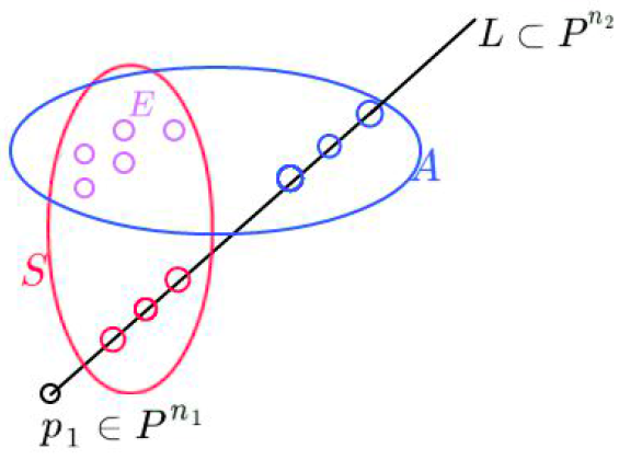
Figure 1. The schemes $S$ and $A$ computes the rank of $p$. $S\cap A=E=\{\hbox{purple dots}\}$, $S=\{\hbox{red}+\hbox{purple dots}\}$, $A=\{\hbox{blue}+\hbox{purple dots}\}$. In the figure we have dropped the “ square brackets ” for $[p]$ to simplify the visualization.

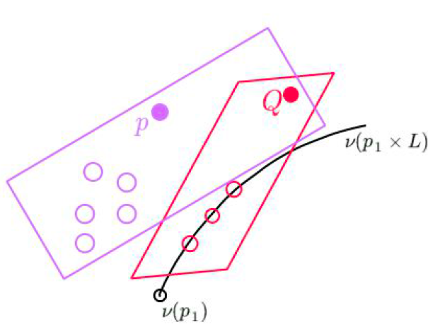
Figure 2. In the figure we have dropped the “ square brackets ” for $[p]$ and $[p_{1}]$ to simplify the visualization and $\nu$ stays for $\nu_{d_{1},d_{2}}$. The point $[p]\in\langle\nu_{d_{1},d_{2}}(E),Q\rangle$ where $\nu_{d_{1},d_{2}}(E)=\{\hbox{purple dots}\}$; $Q\in\langle\nu_{d_{1},d_{1}}(S\setminus E)\rangle$ and $\nu_{d_{1},d_{1}}(S\setminus E)=\{\hbox{red dots}\}$. There is a $g^{1}_{d_{2}+2-b}$ of points in $\nu_{d_{1},d_{2}}([p_{1}]\times L)$ whose span contains $Q$ but such a $Q$ is unique as $E$ is in the decomposition of $p$.

Remark 1.5.

By the classical result of Sylvester (see eg. [18, 10, 13]) in cases (i) and (ii) the set $\mathcal{S}({p})$ is infinite. Cases (i) and (ii) are mutually exclusive (see Remark 1.12).

After having proved Theorem 1.4, we will show the uniqueness result that is described by the following proposition (case in which $p$ depends on both factors).

Proposition 1.6 (Uniqueness of the decomposition).

Take the assumptions of Theorem 1.4 with $\sharp(\cal{S}({p}))\geq 2$ and not in case (iii).

1. To be in case (i) or in case (ii) and the value of the integer $b$ only depends on $p$, not on the choice of $S,A\in\cal{S}({p})$ with $S\neq A$.

2. The $\beta$-curve $T=[p_{1}]\times L$ or the $\alpha$-curve $T=R\times[p_{2}]$ and the set $E:=S\setminus S\cap T=A\setminus A\cap T$ only depend on $[p]$, not the choice of $S,A\in\cal{S}({p})$ with $S\neq A$.

In the next subsection we collect all the proofs of Theorem 1.4 and of Proposition 1.6.

1.1. The proofs of Theorem 1.4 and of Proposition 1.6

Before giving the proof of Theorem 1.4 we need some preliminary Lemma.

Remark 1.7.

Fix $(a_{1},a_{2})\in\mathbb{N}^{2}$, $T\in|\cal{O}_{\mathbb{P}^{1}\times\mathbb{P}^{1}}(1,0)|$ and a zero-dimensional scheme $Z\subset T$. Clearly $T\cong\mathbb{P}^{1}$ and $\cal{O}_{T}(a_{1},a_{2})$ is a line bundle of degree $a_{2}$. Hence $h^{1}\left(T,\cal{I}_{Z,T}(a_{1},a_{2})\right)>0$ if and only if $\deg(Z)\geq a_{2}+2$. Since $h^{i}\left(\cal{O}_{\mathbb{P}^{1}\times\mathbb{P}^{1}}(a_{1}-1,a_{2})\right)=0$ for $i=1,2$, we have $h^{1}\left(T,\cal{I}_{Z,T}(a_{1},a_{2})\right)>0$ if and only if $h^{1}\left(\cal{I}_{Z}(a_{1},a_{2})\right)>0$.

Lemma 1.8.

Fix $F\in|\mathcal{O}_{\mathbb{P}^{1}\times\mathbb{P}^{1}}(1,1)|$ and integers $(a_{1},a_{2})\in\mathbb{N}^{2}$. Let $Z\subset F$. We have $h^{1}(\cal{I}_{Z}(a_{1},a_{2}))>0$ if and only if either $\deg(Z)\geq a_{1}+a_{2}+2$ or there is a proper subcurve $G$ of $F$, say of type $(e_{1},e_{2})$, with $\deg(Z\cap G)\geq e_{2}a_{1}+e_{1}a_{2}+2$.

Proof.

The “ if ” part is true, because if $Z^{\prime}\subseteq Z$, then $h^{1}(\cal{I}_{Z^{\prime}}(a_{1},a_{2}))\leq h^{1}(\cal{I}_{Z}(a_{1},a_{2}))$ and $h^{1}(\cal{I}_{Z}(a_{1},a_{2}))=h^{1}(F,\cal{I}_{Z,F}(a_{1},a_{2}))$.
If $F$ is integral, then the lemma is obvious, because the arithmetic genus of $F$ is 0 and $\deg(\cal{O}_{F}(a_{1},a_{2}))=a_{1}+a_{2}$.
Therefore assume $F=T+G$ with $T\in|\mathcal{O}_{\mathbb{P}^{1}\times\mathbb{P}^{1}}(1,0)|$ and $G\in|\mathcal{O}_{\mathbb{P}^{1}\times\mathbb{P}^{1}}(0,1)|$. If $\deg(Z\cap T)\leq a_{2}+1$, then a residual sequence

$$0\to\cal{I}_{\operatorname{Res}_{T}(Z)}(a_{1}-1,a_{2})\to\cal{I}_{Z}(a_{1},a_{2})\to\cal{I}_{Z\cap T,T}(a_{1},a_{2})\to 0$$

gives $h^{1}\left(\cal{I}_{\operatorname{Res}_{T}(Z)}(a_{1}-1,a_{2})\right)>0$. Since $\operatorname{Res}_{T}(Z)\subset G$, Remark 1.7 gives $\deg(\operatorname{Res}_{T}(Z))\geq a_{1}+1$ and hence $\deg(G\cap Z)\geq a_{1}+1$.
Similarly, by using the other exact sequence

$$0\to\cal{I}_{\operatorname{Res}_{G}(Z)}(a_{1},a_{2}-1)\to\cal{I}_{Z}(a_{1},a_{2})\to\cal{I}_{Z\cap G,G}(a_{1},a_{2})\to 0$$

we get $\deg(\operatorname{Res}_{G}(Z))\geq a_{2}+1$.

Hence $\deg(Z)=\deg(\operatorname{Res}_{G}(Z))+\deg(Z\cap G)\geq a_{1}+a_{2}+2$. ∎

In Lemma 1.10 we will need to perform and inductive procedure. The first step of the induction will be a consequence of the following lemma.

Lemma 1.9.

Fix $(a_{1},a_{2})\in\mathbb{N}^{2}$. Let $Z\subset\mathbb{P}^{1}\times\mathbb{P}^{1}$ be a zero-dimensional scheme such that $\deg(Z)\leq a_{1}+a_{2}+2$, $h^{1}\left(\cal{I}_{Z^{\prime}}(a_{1},a_{2})\right)=0$ for every $Z^{\prime}\subsetneq Z$ and $h^{1}\left(\cal{I}_{Z}(a_{1},a_{2})\right)>0$. Then

• Either $\deg(Z)=a_{2}+2$ and there is $[o]\in\mathbb{P}^{1}$ with $Z\subset\mathbb{P}^{1}\times\{[o]\}$,

• Or $\deg(Z)=a_{1}+2$ and there is $[q]\in\mathbb{P}^{1}$ such that $Z\subset\{[q]\}\times\mathbb{P}^{1}$,

• Or $\deg(Z)=a_{1}+a_{2}+2$ and there is $F\in|\mathcal{O}_{\mathbb{P}^{1}\times\mathbb{P}^{1}}(1,1)|$ such that $Z\subset F$,

• Or $a_{1}=0$ and $\deg(Z)=a_{2}+2$ or $a_{2}=0$ and $\deg(Z)=a_{1}+2$.

Proof.

We use induction on $a_{1}+a_{2}$, the starting case of the induction being the trivial case $a_{1}=a_{2}=0$.

First assume $a_{1}=0$. If there is $[q]\in\mathbb{P}^{1}$ with $\deg(Z\cap(\{[q]\}\times\mathbb{P}^{1}))\geq 2$, then we are done, because $h^{1}\left(\cal{I}_{Z\cap(\{[q]\}\times\mathbb{P}^{1})}(0,a_{2})\right)>0$.
Now assume $\deg(Z\cap(\{[q]\}\times\mathbb{P}^{1}))\leq 1$ for all $[o]\in\mathbb{P}^{1}$. In this case the projection on the first factor $\pi_{1}:\mathbb{P}^{1}\times\mathbb{P}^{1}\rightarrow\mathbb{P}^{1}$ induces an embedding of $Z$ into $\mathbb{P}^{1}$ and we use that $h^{1}\left(\mathbb{P}^{1},\cal{I}_{\pi_{1}(Z),\mathbb{P}^{1}}(a_{2})\right)>0$ if and only if $\deg(\pi_{1}(Z))\geq a_{2}+2$.

Clearly the case $a_{2}=0$ is analogous.

Now assume $a_{1}>0$ and $a_{2}>0$. Fix $D\in|\cal{O}_{\mathbb{P}^{1}\times\mathbb{P}^{1}}(1,1)|$ such that $\deg(D\cap Z)$ is maximal. If $Z\subset D$, then we apply Lemma 1.8 taking $F:=D$ if $\deg(Z)=a_{1}+a_{2}+2$. Hence we may assume $Z\nsubseteq D$.

Since $Z\cap D\subsetneq Z$, we have $h^{1}\left(\cal{I}_{Z\cap D}(a_{1},a_{2})\right)=0$ and hence $h^{1}\left(D,\cal{I}_{Z\cap D}(a_{1},a_{2})\right)=0$. The residual exact sequence of $D$ in $\mathbb{P}^{1}\times\mathbb{P}^{1}$

$$0\to\cal{I}_{\operatorname{Res}_{D}(Z)}(a_{1}-1,a_{2}-1)\to\cal{I}_{Z}(a_{1},a_{2})\to\cal{I}_{Z\cap D,D}(a_{1},a_{2})\to 0$$

gives $h^{1}\left(\cal{I}_{\operatorname{Res}_{D}(Z)}(a_{1}-1,a_{2}-1)\right)>0$. We have $\deg({\operatorname{Res}_{D}(Z)})=\deg(Z)-\deg(D\cap Z)$. Since $h^{0}\left(\cal{O}_{\mathbb{P}^{1}\times\mathbb{P}^{1}}(1,1)\right)=4$, we have $\deg(D\cap Z)\geq 3$. Hence $\deg({\operatorname{Res}_{D}(Z)})\leq(a_{1}-1)+(a_{2}-1)+1$. Let $W\subseteq\operatorname{Res}_{D}(Z)$ be a minimal subscheme such that $h^{1}\left(\cal{I}_{W}(a_{1}-1,a_{2}-1)\right)>0$. Since $\deg(W)\leq(a_{1}-1)+(a_{2}-1)+1$, the inductive assumption gives that

1. Either $a_{1}=1$ and $\deg(W)\geq(a_{2}-1)+2$,

2. Or $a_{2}=1$ and $\deg(W)\geq(a_{1}-1)+2$,

3. Or $a_{1}\geq 2$ and there is $[o]\in\mathbb{P}^{1}$ with $\deg(W\cap\mathbb{P}^{1}\times\{[o]\})\geq a_{2}+1$,

4. Or $a_{2}\geq 2$ and there is $[q]\in\mathbb{P}^{1}$ such that $\deg(W\cap\{[q]\}\times\mathbb{P}^{1})\geq a_{1}+1$.

Note that in each case the inequality holds if we take $\operatorname{Res}_{D}(Z)$ instead of $W$.

First assume $a_{1}=1$ and $\deg({\operatorname{Res}_{D}(Z)})\geq a_{2}+1$. Since $\deg(Z)\leq a_{1}+a_{2}+2=a_{2}+3$, we get $\deg(Z\cap D)\leq 2$, a contradiction.

In the same way we conclude if $a_{2}=1$ and $\deg({\operatorname{Res}_{D}(Z)})\geq a_{1}+1$.

Now assume $a_{1}\geq 2$ and the existence of $[o]\in\mathbb{P}^{1}$ with $\deg\left({\operatorname{Res}_{D}(Z)}\cap\mathbb{P}^{1}\times\{[o]\}\right)\geq a_{2}+1$. $\hbox{Set }R:=\mathbb{P}^{1}\times\{[o]\}\in|\cal{O}_{\mathbb{P}^{1}\times\mathbb{P}^{1}}(0,1)|$. If $\deg(R\cap Z)\geq a_{2}+2$, then we are done. Hence we may assume $\deg(R\cap Z)\leq a_{2}+1$. Since $Z\supset{\operatorname{Res}_{D}(Z)}$ and $\deg({\operatorname{Res}_{D}(Z)}\cap R)\geq a_{2}+1$, we get $Z\cap R=Z\cap{\operatorname{Res}_{D}(Z)}$ and $\deg(Z\cap R)=a_{2}+1$.

We have $\deg({\operatorname{Res}_{R}(Z)})\leq a_{1}+1$. The residual exact sequence of $R$

$$0\to\cal{I}_{\operatorname{Res}_{R}(Z)}(a_{1},a_{2}-1)\to\cal{I}_{Z}(a_{1},a_{2})\to\cal{I}_{Z\cap R,R}(a_{1},a_{2})\to 0$$

gives $h^{1}\left(\cal{I}_{\operatorname{Res}_{R}(Z)}(a_{1},a_{2}-1)\right)>0$.

Let $W^{\prime}\subseteq\operatorname{Res}_{R}(Z)$ be a minimal subscheme with $h^{1}\left(\cal{I}_{W^{\prime}}(a_{1},a_{2}-1)\right)>0$. The inductive assumption gives $\deg({\operatorname{Res}_{R}(Z)})\geq\deg(W^{\prime})\geq 2+\min\{a_{1},a_{2}-1\}$. Since $\deg({\operatorname{Res}_{R}(Z)})\leq a_{1}+1$, we get $a_{2}\leq a_{1}-2$. Take $L\in|\cal{O}_{\mathbb{P}^{1}\times\mathbb{P}^{1}}(1,0)|$ such that $\deg(L\cap Z)$ is maximal. Since $h^{1}\left(\cal{I}_{Z^{\prime}}(a_{1},a_{2})\right)=0$ for all $Z^{\prime}\subsetneq Z$, either $Z\subset L$ (and hence $\deg(Z)=a_{2}+2$ and the lemma is true) or $\deg(L\cap Z)\leq a_{2}+1$. We may assume that $\deg(L\cap Z)\leq a_{2}+1$ and hence $h^{1}\left(L,\cal{I}_{L\cap Z}(a_{1},a_{2})\right)=0$. The residual exact sequence of $L$ gives $h^{1}\left(\cal{I}_{\operatorname{Res}_{L}(Z)}(a_{1}-1,a_{2})\right)>0$. Let $W_{1}\subseteq\operatorname{Res}_{L}(Z)$ be a minimal subscheme such that $h^{1}\left(\cal{I}_{W_{1}}(a_{1}-1,a_{2})\right)>0$. Since $a_{1}-1>0$, the inductive assumption gives that either $\deg(W_{1})=a_{1}+1$ and $W_{1}$ is contained in $R_{1}\in|\cal{O}_{\mathbb{P}^{1}\times\mathbb{P}^{1}}(1,0)|$ or $\deg(W_{1})=a_{2}+2$ and $W_{1}$ is contained in an element of $|\cal{O}_{\mathbb{P}^{1}\times\mathbb{P}^{1}}(0,1)|$ or $\deg(W_{1})=a_{1}+a_{2}+1$ and $W_{1}$ is contained in an element of $|\cal{O}_{\mathbb{P}^{1}\times\mathbb{P}^{1}}(1,1)|$. In the latter case we get $\deg(D\cap Z)\geq a_{1}+a_{2}+1$ and so $\deg(\operatorname{Res}_{D}(Z))\leq 1$ and hence $h^{1}(\cal{I}_{\operatorname{Res}_{D}(Z)}(a_{1}-1,a_{2}-1))=0$, a contradiction. In the second case we get that we are in the first case of the lemma. Now assume the existence of $R_{1}\in|\cal{O}_{\mathbb{P}^{1}\times\mathbb{P}^{1}}(1,0)|$ such that $\deg(R_{1}\cap W_{1})\geq a_{1}+1$. Since $W_{1}\subseteq\operatorname{Res}_{L}(Z)\subset Z$, the maximality property of the integer $\deg(L\cap Z)$ gives $\deg(L\cap Z)\geq a_{1}+1$. Therefore $\deg(Z)\geq\deg(L\cap Z)+\deg(\operatorname{Res}_{L}(Z))\geq 2a_{1}+2$, contradicting the inequalities $a_{2}\leq a_{1}-2$ and $\deg(Z)\leq a_{1}+a_{2}+2$.

The same proof works if $a_{2}\geq 2$ and there is $[q]\in\mathbb{P}^{1}$ such that $\deg({\operatorname{Res}_{F}(Z)}\cap\{Q\}\times\mathbb{P}^{1})\geq a_{1}+1$. ∎

Lemma 1.10.

Let $\Gamma\subset\mathbb{P}^{n_{1}}\times\mathbb{P}^{n_{2}}$ be zero-dimensional scheme such that $\deg(\Gamma)\leq d_{1}+d_{2}+1$, $h^{1}(\cal{I}_{\Gamma^{\prime}}(d_{1},d_{2}))=0$ for all $\Gamma^{\prime}\subsetneq\Gamma$ and $h^{1}(\cal{I}_{\Gamma}(d_{1},d_{2}))>0$ with $d_{1},d_{2}>0$. Then either there is $[p_{1}]\in\mathbb{P}^{n_{1}}$ such that $\Gamma\subset[p_{1}]\times\mathbb{P}^{n_{2}}$ or there is $[p_{2}]\in\mathbb{P}^{n_{2}}$ such that $h^{1}(\cal{I}_{\mathbb{P}^{n_{1}}\times[p_{2}]}(d_{1},d_{2}))>0$. If the second case occurs and $d_{2}\geq d_{1}$, then $\deg(\Gamma)=d_{2}+2$ and there is a $\beta$-line $T$ such that $\Gamma\subset T$.

Proof.

The last sentence follows from the first part of the lemma by [10, Lemma 34], because $\deg(\Gamma)\leq 2d_{2}+1$ if $d_{1}\leq d_{2}$. Hence it is sufficient to prove the first part. By assumption $h^{1}(\cal{I}_{\Gamma^{\prime}}(d_{1},d_{2}))=0$ for all $\Gamma^{\prime}\subsetneq\Gamma$. With this assumption we need to prove that $\Gamma$ is contained in one of the slices of $\mathbb{P}^{n_{1}}\times\mathbb{P}^{n_{2}}$. By Lemma 1.8 and Lemma 1.9 we may assume $n_{1}+n_{2}>2$ and use induction on the integer $n_{1}+n_{2}$. We also use induction on the integer $d_{1}+d_{2}$, the case $(d_{1},d_{2})=(1,1)$ being obviously true, because $\deg(\Gamma)\leq 3$ (but note that as stated the result would be wrong if $d_{2}=0$ and $n_{1}\geq 2$). With no loss of generality for the firs part we may assume $d_{2}\geq d_{1}$ and in particular $d_{2}\geq 2$.

Take $D_{1}\in|\cal{O}_{\mathbb{P}^{n_{1}}\times\mathbb{P}^{n_{2}}}(0,1)|$ such that $f_{1}:=\deg(\Gamma\cap D_{1})$ is maximal. Since obviously $h^{0}(\cal{O}_{\mathbb{P}^{n_{1}}\times\mathbb{P}^{n_{2}}}(0,1))=n_{2}+1$, we have $f_{1}\geq n_{2}>0$. If $h^{1}\left(D_{1},\mathcal{I}_{\Gamma\cap D_{1}}(d_{1},d_{2})\right)>0$, then we may use the inductive assumption on the integer $n_{1}+n_{2}$. Hence we assume that $h^{1}\left(D_{1},\mathcal{I}_{\Gamma\cap D_{1}}(d_{1},d_{2})\right)=0$. Therefore by the Castelnuovo’s sequence

$$0\to\cal{I}_{\operatorname{Res}_{D_{1}}(\Gamma)}(d_{1},d_{2}-1)\to\cal{I}_{\Gamma}(d_{1},d_{2})\to\cal{I}_{\Gamma\cap{D_{1}},{D_{1}}}(d_{1},d_{2})\to 0$$

we have $h^{1}\left(\cal{I}_{\mathrm{Res}_{D_{1}}(\Gamma)}(d_{1},d_{2}-1)\right)=0$.
Now, let $\pi_{i}:\mathbb{P}^{n_{1}}\times\mathbb{P}^{n_{2}}\to\mathbb{P}^{n_{i}}$ be the projection on the $i$-th factor for $i=1,2$. Since $f_{1}>0$ and $d_{2}-1>0$, the inductive assumption gives that either there is a point $[p_{1}]\in\mathbb{P}^{n_{1}}$ such that $h^{1}\left(\cal{I}_{\mathrm{Res}_{D_{1}}(\Gamma)\cap\pi_{1}^{-1}([p_{1}])}(d_{1},d_{2}-1)\right)>0$ or there is a point $[p_{2}]\in\mathbb{P}^{n_{2}}$ such that $h^{1}\left(\cal{I}_{\mathrm{Res}_{D_{1}}(\Gamma)\cap\pi_{2}^{-1}([p_{2}])}(d_{1},d_{2}-1)\right)>0$. If $[p_{2}]$ exists, then we are done, since $\Gamma\supseteq\mathrm{Res}_{D_{1}}(\Gamma)$.

Now assume that such a $[p_{2}]$ does not exist while suppose the existence of $[p_{1}]\in\mathbb{P}^{n_{1}}$ such that $h^{1}\left(\cal{I}_{\mathrm{Res}_{D_{1}}(\Gamma)\cap\pi_{1}^{-1}([p_{1}])}(d_{1},d_{2}-1)\right)>0$. Since $f_{1}>0$ and $d_{2}\geq d_{1}$ we have $\deg(\mathrm{Res}_{D_{1}}(\Gamma))\leq 2d_{2}$. By [10, Lemma 34] there is a $\beta$-line $T\subset\pi_{1}^{-1}([p_{1}])$ such that $\deg(T\cap\mathrm{Res}_{D_{1}}(\Gamma))\geq d_{2}+1$.
If $n_{2}\geq 2$, there is $D\in|\cal{O}_{\mathbb{P}^{n_{1}}\times\mathbb{P}^{n_{2}}}(0,1)|$ containing $T$ and hence $f_{1}\geq d_{2}+1$. We get that $\deg(\Gamma)\geq 2d_{2}+2$ which contradicts the hypothesis.
Now assume $n_{2}=1$ and hence $n_{1}\geq 2$. Fix $M_{1}\in|\cal{O}_{\mathbb{P}^{n_{1}}\times\mathbb{P}^{n_{2}}}(1,0)|$ such that $g:=\deg(M_{1}\cap\Gamma)$ is maximal. The existence of the $\beta$-line $T$ such that $\deg(T\cap\mathrm{Res}_{D_{1}}(\Gamma))\geq d_{2}+1$ gives that $g\geq d_{2}+n_{1}-1$.
If $h^{1}\left(M_{1},\mathcal{I}_{\Gamma\cap M_{1}}(d_{1},d_{2})\right)>0$, then, again, we can use the inductive assumption on the integer $n_{1}+n_{2}$.
Hence we may assume that $h^{1}\left(M_{1},\mathcal{I}_{\Gamma\cap M_{1}}(d_{1},d_{2})\right)=0$. The Castelnuovo’s sequence gives $h^{1}\left(\mathcal{I}_{\mathrm{Res}_{M_{1}}(\Gamma)}(d_{1}-1,d_{2})\right)>0$.
If $d_{1}=1$, then we get $\deg(\mathrm{Res}_{M_{1}}(\Gamma))\geq 2$ and hence $\deg(\Gamma)\geq g+2\geq d_{2}+n_{1}+1>d_{1}+d_{2}+1$, which contradicts the hypothesis on the degree of $\Gamma$.
If $d_{1}\geq 2$, the inductive assumption gives $\deg(\operatorname{Res}_{M_{1}}(\Gamma))\geq d_{1}+2$ and than we have $\deg(\Gamma)\geq d_{2}+n_{1}-1+d_{1}+2\geq d_{1}+d_{2}+2$, which is again a contradiction. ∎

The case $n=2$ of the following observation is [7, Lemma 4.4]; the case $n>2$ follows by induction on $n$ taking a hyperplane $H\subset\mathbb{P}^{n}$ such that $\deg(Z\cap H)$ is maximal.

Remark 1.11.

Let $Z\subset\mathbb{P}^{n}$ be a finite set such that $h^{1}(\cal{I}_{Z}(t))>0$ and $\deg(Z)\leq 2t+2$. Then either there is a line $L\subset\mathbb{P}^{n}$ with $\deg(L\cap Z)\geq d+2$ or $\deg(Z)=2t+2$ and there is a reduced conic $C\subset\mathbb{P}^{n}$ such that $Z\subset C$.

Remark 1.12.

Take $\Gamma,d_{1},d_{2},n_{1},n_{2}$ as in Lemma 1.10 and assume the existence of a $\beta$-line $\mathcal{B}$ such that $h^{1}(\cal{I}_{\Gamma\cap\mathcal{B}}(d_{1},d_{2}))>0$, i.e. such that $\deg(\Gamma\cap\mathcal{B})\geq d_{1}+2$. Fix any $\alpha$-line $\mathcal{A}$ . Since $\deg(\mathcal{B}\cap\mathcal{A})\leq 1$, we have $\deg(\Gamma\cap\mathcal{A})\leq d_{1}+d_{2}+1-(d_{1}+2)+1=d_{2}$.

We are now ready to prove the decomposition Theorem 1.4.

Proof of Theorem 1.4:.

Since the proof of this theorem is quite structured, we decided to divide it in various claims in order to facilitate the reading and to equip each one of them with a figure.

First of all remark that we have $1+2\min\{d_{1},d_{2}\}\leq 1+d_{1}+d_{2}$ and hence with any of the assumptions of Theorem 1.4 we could get $2r({p})\leq 1+d_{1}+d_{2}$.

Let’s start by fixing two different sets of points $S,A\in\cal{S}({p})$ computing the rank of $p$. Then let

$$S^{\prime\prime}:=S\cap A.$$

as in Figure 3.

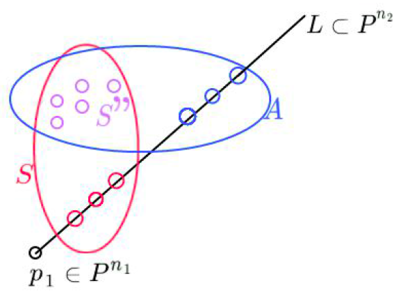
Figure 3. In the figure we have dropped the “ square brackets ” for $[p]$ to simplify the visualization.

Since $S$ and $A$ are different, then $S^{\prime\prime}$ is a proper subset of both $S$ and $A$, i.e. $S^{\prime\prime}\subsetneq S,A$.

Claim 1: Take any subset of points $G\subseteq S^{\prime\prime}$. There is a unique point $Q\in\langle\nu_{d_{1},d_{2}}(A\setminus G)\rangle\cap\langle\nu_{d_{1},d_{2}}(S\setminus G)\rangle$ such that $[p]\in\langle\nu_{d_{1},d_{2}}(G)\cup\{Q\}\rangle$ and $r(Q)=\sharp(S)-\sharp(G)$ (this is illustrated in Figure 4).

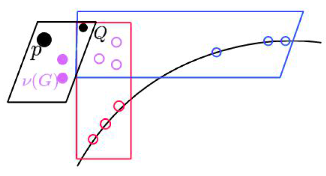
Figure 4. In the figure we have dropped the “ square brackets ” for $[p]$ to simplify the visualization and $\nu$ stays for $\nu_{d_{1},d_{2}}$.

Proof of Claim 1: If $G=\emptyset$, then this claim is trivial (it is sufficient to take $Q=[p]$). So we may assume $G\neq\emptyset$.

Since $\nu_{d_{1},d_{2}}(S)$ is linearly independent, we have $\langle\nu_{d_{1},d_{2}}(S)\rangle\cap\langle\nu_{d_{1},d_{2}}(A)\rangle=\langle\nu_{d_{1},d_{2}}(S\setminus G)\rangle\cap\langle\nu_{d_{1},d_{2}}(A\setminus G)\rangle+\langle\nu_{d_{1},d_{2}}(G)\rangle$ and this is a direct decomposition. Since $[p]\notin\langle\nu_{d_{1},d_{2}}(G)\rangle$ for any $G\subsetneq S$, we have $[p]\notin\langle\nu_{d_{1},d_{2}}(S^{\prime\prime})\rangle$ and so there is a unique $Q\in\langle\nu_{d_{1},d_{2}}(A\setminus G)\rangle\cap\langle\nu_{d_{1},d_{2}}(S\setminus G)\rangle$ such that $[p]\in\langle\nu_{d_{1},d_{2}}(G)\cup\{Q\}\rangle$. Since $Q\in\langle\nu_{d_{1},d_{2}}(S\setminus G)\rangle$, we have $r(Q)\leq\sharp(S)-\sharp(G)$. Since $[p]$ is in the linear span of $Q$ and $\nu_{d_{1},d_{2}}(G)$, we have $r({p})\leq r(Q)+\sharp(G)$. Hence $r(Q)=\sharp(S)-\sharp(G)$.∎

Now, set

(3) $$B:=A\cup S.$$

Since $2r({p})\leq 1+d_{1}+d_{2}$, we have $\sharp(B)\leq 1+d_{1}+d_{2}$. Since $A\nsubseteq S$ and $S\nsubseteq A$, we have $h^{1}(\cal{I}_{B}(d_{1},d_{2}))>0$ ([4, Lemma 1]). By Lemma 1.10 there is either a $\beta$-slice $\mathbb{B}$ such that $h^{1}(\cal{I}_{B\cap\mathbb{B}}(d_{1},d_{2}))>0$ or an $\alpha$-slice $\mathbb{A}$ such that $h^{1}(\cal{I}_{B\cap\mathbb{A}}(d_{1},d_{2}))>0$. We assume the existence of the $\beta$-slice $\mathbb{B}=[p_{1}]\times\mathbb{P}^{n_{2}}$, because the case of the $\alpha$-slice is analogous. We first assume that $\deg(\Gamma\cap\mathbb{B})\geq 2d_{2}+2$. We get that we are in case (a) with $d_{1}\geq d_{2}$ and that $B\subset\mathbb{B}$. By Remark 1.11 we have $n_{2}\geq 2$ and there is a reduced conic $C\subset\mathbb{P}^{n_{2}}$ such that $[p]\in\nu_{d_{1},d_{2}}([p_{1}]\times C)$ and $A\cup S\subset[p_{1}]\times C$, i.e. we are in case (iii). Now assume $\deg(\Gamma\cap\mathbb{B})\leq 2d_{2}+1$. By [10, Lemma 34] there is a line $L\subset\mathbb{P}^{n_{2}}$ such that $\deg(\Gamma\cap[p_{1}]\cap L)\geq d_{2}+2$. Set $\mathcal{B}:=[p_{1}]\times L$.

Set:

• $A^{\prime}:=A\cap\mathbb{B}$,

• $S^{\prime}:=S\cap\mathbb{B}$ and

• $B^{\prime}:=B\cap\mathbb{B}=A^{\prime}\cup S^{\prime}$.

Since $h^{1}(\mathbb{B},\cal{I}_{B^{\prime}}(d_{1},d_{2}))>0$, we have $\sharp(B^{\prime})\geq d_{2}+2$ and equality holds only if $B^{\prime}$ is contained in a line.

Claim 2: We have that $A\setminus A^{\prime}=S\setminus S^{\prime}$ (illustrated in Figure 5).

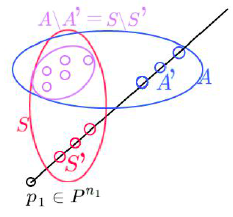
Figure 5. In the figure we have dropped the “ square brackets ” for $[p]$ to simplify the visualization.

Proof of Claim 2: Let $D\subset\mathbb{P}^{n_{1}}$ be a general hyperplane containing $[p_{1}]$. For a general $D$ we have $D\cap B=B^{\prime}$.

Consider the residual exact sequence of $D$:

(4) $$0\to\cal{I}_{B\setminus B^{\prime}}(d_{1}-1,d_{2})\to\cal{I}_{B}(d_{1},d_{2})\to\cal{I}_{B^{\prime},D}(d_{1},d_{2})\to 0.$$

If $h^{1}\left(\cal{I}_{B\setminus B^{\prime}}(d_{1}-1,d_{2})\right)=0$, then, from [6, Lemma 5.1], we immediately get that $A\setminus A^{\prime}=S\setminus S^{\prime}$.

Now assume $h^{1}\left(\cal{I}_{B\setminus B^{\prime}}(d_{1}-1,d_{2})\right)>0$. Since $\sharp(B)\leq d_{1}+d_{2}+1$ and $\sharp(B^{\prime})\geq d_{2}+2$, we have $\sharp(B\setminus B^{\prime})\leq d_{1}-1$. Hence $h^{1}\left(\cal{I}_{B\setminus B^{\prime}}(d_{1}-1,d_{2})\right)=0$ if $d_{1}=1$. Therefore we may assume $d_{1}-1>0$. By Lemma 1.10 (with $\Gamma$ being $B$) we have $d_{2}\leq d_{1}-3$ and $\sharp(B\setminus B^{\prime})\geq d_{2}+2$ (one can also apply Remark 1.12 with $\Gamma=B$ and $\mathcal{B}=N$), contradicting the assumption $\sharp(B)\geq 2d_{2}$ when $d_{2}\leq d_{1}-3$.∎

Now if we apply Claim 1 to the set $G:=A\setminus A^{\prime}$, we get a unique $Q\in\langle\nu_{d_{1},d_{2}}([p_{1}]\times\mathbb{P}^{n_{2}})\rangle$ with $A^{\prime}\in\cal{S}(Q)$ and $[p]\in\langle\nu_{d_{1},d_{2}}(G)\cup\{Q\}\rangle$.
Let $L\subseteq\mathbb{P}^{n_{2}}$ be a line such $h^{1}\left(\cal{I}_{B\cap([p_{1}]\times L)}(d_{1},d_{2})\right)>0$. With $\mathcal{B}=[p_{1}]\times L$, set:

• $A_{1}:=A\cap\mathcal{B}$,

• $S_{1}:=S\cap\mathcal{B}$ and

• $B_{1}:=A_{1}+S_{1}$.

Claim 3: We have $A\setminus A_{1}=S\setminus S_{1}$ (illustrated in Figure 6).

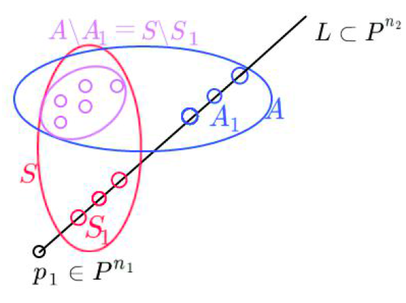
Figure 6. In the figure we have dropped the “ square brackets ” for $[p]$ to simplify the visualization.

Proof of Claim 3: If $n_{2}=1$, then $L=\mathbb{P}^{n_{2}}$, $A_{1}=A^{\prime}$ and $S_{1}=S^{\prime}$ and we may apply Claim 2.

Now assume $n_{2}\geq 2$ and fix $H\in|\cal{O}_{\mathbb{P}^{n_{1}}\times\mathbb{P}^{n_{2}}}(0,1)|$ with $L\subset H$ and $H$ general. For a general $H$ we have $S\cap H=S_{1}$ and $A\cap H=A_{1}$. Consider the residual exact sequence of $H$:

(5) $$0\to\cal{I}_{B\setminus B_{1}}(d_{1},d_{2}-1)\to\cal{I}_{B}(d_{1},d_{2})\to\cal{I}_{B_{1},H}(d_{1},d_{2})\to 0.$$

Since $\sharp(B_{1})\geq d_{2}+2$, we have $\sharp(B\setminus B_{1})\leq d_{1}-1$.

If $h^{1}(\cal{I}_{B\setminus B_{1}}(d_{1},d_{2}-1))=0$, then [6, Lemma 5.1] gives $A\setminus A_{1}=S\setminus A_{1}$.

Now assume $h^{1}\left(\cal{I}_{B\setminus B_{1}}(d_{1},d_{2}-1)\right)>0$. First assume $d_{2}\geq 2$. Lemma 1.9 for the integers $(a_{1},a_{2})=(d_{1},d_{2}-1)$ gives $\sharp(B\setminus B_{1})\geq 2+\min\{d_{1},d_{2}-1\}$. Since $\sharp(B\setminus B_{1})\leq d_{1}-1$, we first get $d_{2}\leq d_{1}$ and then (since $|d_{1}-d_{2}|\leq 2$, $\sharp(B)\leq 1+d_{1}+d_{2}$ and $\sharp(B_{1})\geq d_{2}+2$) we get $\sharp(B)=1+d_{1}+d_{2}$, $\sharp(B_{1})=d_{2}+2$ and $d_{1}=d_{2}+2$. Since we are necessary in case (a) $\sharp(B)\leq 2r({p})\leq 1+d_{1}+d_{2}$, we get $2r({p})=1+d_{1}+d_{2}=3+2d_{2}$, a contradiction (because $3+2d_{2}$ is odd). Now assume $d_{2}=1$ and hence $d_{1}\leq 3$. Since $2r({p})\leq 1+d_{1}+d_{2}\leq 5$, we have $r({p})\leq 2$. Since $B\supseteq B_{1}$ and $\sharp(B_{1})\geq d_{2}+2$, we get a contradiction. ∎

Now set

$$E:=S\setminus S_{1}.$$

as in Figure 7.

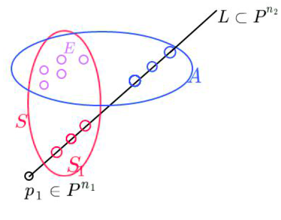
Figure 7. In the figure we have dropped the “ square brackets ” for $[p]$ to simplify the visualization.

By Claim 1 applied to the set $G:=E$, we have $A_{1},S_{1}\in\cal{S}(Q)$ and $A_{1}\neq S_{1}$. By the famous theorem of Sylvester [18, 10] either $d_{2}$ is even and $\sharp(A_{1})=\sharp(S_{1})=(d_{2}+2)/2$ or the border rank $b$ of $Q$ is smaller that the rank of $Q$, $2\leq b\leq\lfloor d_{2}/2\rfloor$ and $r(Q)=d_{2}+2-b$. In the latter case we are in case (i) of Theorem 1.4 with $b$ the border rank. If $\sharp(S_{1})=(d_{2}+2)/2$ we are in case (i) with $b=(d_{2}+2)/2$. Both cases are contained in case (i) of Theorem 1.4.∎

With the proof of Theorem 1.4 done, we can now show the uniqueness part and prove Proposition 1.6.

Proof of Proposition 1.6:.

Fix $S,A,S^{\prime},A^{\prime}\in\cal{S}({p})$ with $S\neq A$, $S^{\prime}\neq A^{\prime}$ and $\{S,A\}\neq\{S^{\prime},A^{\prime}\}$. With no loss of generality we may assume that $(S,A)$ is associated to the $\beta$-line $T=[p_{1}]\times L$, i.e. we are in case (i) of Theorem 1.4.

1. First assume $\{S,A\}\cap\{S^{\prime},A^{\prime}\}\neq\emptyset$, say $A=A^{\prime}$ ($S=S^{\prime}$ will be analogous).

   In the contest of Theorem 1.4, assume that $(S^{\prime},A)$ is associated to a $\beta$-line $T^{\prime}$, an integer $b^{\prime}$ and a set $E^{\prime}=S^{\prime}\setminus S^{\prime}\cap T^{\prime}=A\setminus A\cap T^{\prime}$.

   Clearly, since $A=A^{\prime}$ and since they are both contained in a line ($T$ and $T^{\prime}$ respectively) the two lines have to be the same: $T=T^{\prime}$. This implies that $E=A\setminus A\cap T=E^{\prime}$, therefore in this case there is nothing to prove.

2. Now assume $\{S,A\}\cap\{S^{\prime},A^{\prime}\}=\emptyset$. We can apply step (1) to the two pairs $(S,A)$ and $(S,A^{\prime})$ (resp. the two pairs $(S,A)$ and $(S^{\prime},A)$) and get that $A^{\prime}\setminus A^{\prime}\cap T=E$ (resp. $S^{\prime}\setminus S^{\prime}\cap T=E$). Therefore $S^{\prime}\cap A^{\prime}\supseteq E=S\cap A$. By symmetry, we also have that $S^{\prime}\cap A^{\prime}=S\cap A$. If $(S^{\prime},A^{\prime})$ is associated to a curve $T^{\prime}$ and the integer $b^{\prime}$, then $b=b^{\prime}$.

∎

1.2. A trivial bound for $\rho^{\prime}(X)$ in the case of Segre-Veronese varieties

In the Introduction, in Definition 0.1, we introduced $\rho^{\prime}(X)$ to be the maximal integer $t$ such that any subset of $X$ with cardinality $t$ is linearly independent. Then we stated as a general fact that if $X$ is the Segre-Veronese variety of $k$ factors, i.e. $X=S_{d_{1},\ldots,d_{k}}(V_{1},\ldots,V_{k})$ is the embedding of $\mathbb{P}(V_{1})\times\cdots\times\mathbb{P}(V_{k})$ into $\mathbb{P}(S^{d_{1}}V_{1}\otimes\cdots\otimes S^{d_{k}}V_{k})$ induced by the complete linear system $|\mathcal{O}_{\mathbb{P}(V_{1})\times\cdots\times\mathbb{P}(V_{k})}(d_{1},\ldots,d_{k})|$, then $\rho^{\prime}(X)=1+\min_{1\leq i\leq k}\{d_{i}\}$ (Lemma 1.13). Unfortunately we cannot find a precise reference for this fact, but since it is quite easy to be shown, we include the proof for sake of completeness.

Lemma 1.13.

Let $X$ be the Segre-Veronese embedding of $\mathbb{P}^{n_{1}}\times\cdots\times\mathbb{P}^{n_{k}}$ into $\mathbb{P}(S^{d_{1}}V_{1}\otimes\cdots\otimes S^{d_{k}}V_{k})$ by the linear system $|\cal{O}_{\mathbb{P}^{n_{1}}\times\cdots\times\mathbb{P}^{n_{k}}}(d_{1},\dots,d_{k})|$. Then $\rho^{\prime}(X)=1+\min_{1\leq i\leq k}\{d_{i}\}$.

Proof.

With no loss of generality we may assume $d_{i}\geq d_{1}$ for all $i$.
Fix a line $L\subseteq\mathbb{P}^{n_{1}}$ and $O_{i}\in\mathbb{P}^{n_{i}}$, $i=2,\dots,k$. Take $E\subset L$ with $\sharp(E)=d_{1}+2$ and set $F:=E\times\{O_{2}\}\times\cdots\times\{O_{k}\}$.
Since $h^{1}({\mathbb{P}^{n_{1}}\times\cdots\times\mathbb{P}^{n_{k}}},\cal{I}_{F}(d_{1},\dots,d_{k}))=h^{1}(\mathbb{P}^{n_{1}},\cal{I}_{E}(d_{1}))=h^{1}(L,\cal{I}_{E}(d_{1}))=1$, we have $\rho^{\prime}(X)\leq 1+\min_{1\leq i\leq k}\{d_{i}\}$.

To prove the lemma it is sufficient to show that

$$h^{1}({\mathbb{P}^{n_{1}}\times\cdots\times\mathbb{P}^{n_{k}}},\cal{I}_{S}(d_{1},\dots,d_{k}))=0$$

for every set $S\subset{\mathbb{P}^{n_{1}}\times\cdots\times\mathbb{P}^{n_{k}}}$ with $\sharp(S)\leq d_{1}+1$.
Order the points $p_{1},\dots,p_{x}$, $x\leq d_{1}+1$, of $S$. Set $S_{0}:=\emptyset$ and $S_{y}=\{p_{1},\dots,p_{y}\}$. Since $\cal{O}_{\mathbb{P}^{n_{1}}\times\cdots\times\mathbb{P}^{n_{k}}}(1,\dots,1)$ is very ample, for each $i=1,\dots,x-1$ there is $H_{i}\in|\cal{O}_{\mathbb{P}^{n_{1}}\times\cdots\times\mathbb{P}^{n_{k}}}(1,\dots,1)|$ with $p_{i}\in H_{i}$ and $p_{j}\notin H_{i}$ for all $j\neq i$. If $d_{i}=1$ for all $i$, then set $M:=\emptyset$. If $d_{i}\neq 1$ for some $i$, let $M\in|\cal{O}_{\mathbb{P}^{n_{1}}\times\cdots\times\mathbb{P}^{n_{k}}}(d_{1}-1,\dots,d_{k}-1)|$ with $M\cap S=\emptyset$. The divisors $H_{1}+M,\dots,H_{x-1}+M$ give $h^{0}({\mathbb{P}^{n_{1}}\times\cdots\times\mathbb{P}^{n_{k}}},\cal{I}_{S_{y}}(d_{1},\dots,d_{k}))=h^{0}({\mathbb{P}^{n_{1}}\times\cdots\times\mathbb{P}^{n_{k}}},\cal{I}_{S_{y-1}}(d_{1},\dots,d_{k}))-1$ for $i=1,\dots,x$. Hence $h^{1}(\cal{I}_{S}(d_{1},\dots,d_{k}))=0$. ∎

2. Rank on the tangential variety of Segre-Veronese varieties

First of all in this section we will consider the Segre-Veronese variety
$S_{d_{1},\ldots,d_{k}}(V_{1},\ldots,V_{k})$ of any number of factors. Then we will describe the rank of multi-homogeneous polynomials (partially symmetric tensors) that can be written as a limit of a sequence of rank 2 multi-homogeneous polynomials (partially symmetric tensors). If $p\in S^{d_{1}}V_{1}^{*}\otimes\cdots\otimes S^{d_{k}}V_{k}^{*}$ is one of those polynomials, one says that $[p]$ has border rank 2. To be more precise, let

$$\sigma_{2}(S_{d_{1},\ldots,d_{k}}(V_{1},\ldots,V_{k}))=\overline{\bigcup_{[p_{1}],[p_{2}]\in S_{d_{1},\ldots,d_{k}}(V_{1},\ldots,V_{k})}\langle[p_{1}],[p_{2}]\rangle}$$

be the secant variety to $S_{d_{1},\ldots,d_{k}}(V_{1},\ldots,V_{k})$.
Clearly $S_{d_{1},\ldots,d_{k}}(V_{1},\ldots,V_{k})\subset\sigma_{2}(S_{d_{1},\ldots,d_{k}}(V_{1},\ldots,V_{k}))$.
An element in $\sigma_{2}(S_{d_{1},\ldots,d_{k}}(V_{1},\ldots,V_{k}))$ that is not in $S_{d_{1},\ldots,d_{k}}(V_{1},\ldots,V_{k})$ is either a projective class of a multi-homogeneous polynomial (partially symmetric tensor) of rank 2, or it is the limit of a sequence of rank 2 elements. Clearly, from the point of view of the knowledge of the rank, the only interesting case is the one of points that are limit of rank 2 elements. Those represent a closed subvariety of $\sigma_{2}(S_{d_{1},\ldots,d_{k}}(V_{1},\ldots,V_{k}))$ that we indicate with $\tau(S_{d_{1},\ldots,d_{k}}(V_{1},\ldots,V_{k}))$ and that is the tangential variety of $S_{d_{1},\ldots,d_{k}}(V_{1},\ldots,V_{k})$:

$$\tau(S_{d_{1},\ldots,d_{k}}(V_{1},\ldots,V_{k}))=\overline{\bigcup_{[p]\in S_{d_{1},\ldots,d_{k}}(V_{1},\ldots,V_{k})}T_{[p]}(S_{d_{1},\ldots,d_{k}}(V_{1},\ldots,V_{k}))}.$$

Here we prove the following theorem.

Theorem 2.1.

The rank of $[p]\in\tau(S_{d_{1},\ldots,d_{k}}(V_{1},\ldots,V_{k}))$ is

$$r_{d_{1},\ldots,d_{k}}(p)=\sum_{i=1}^{h}d_{i}$$

if $V_{1}^{*}=K[x_{1,0},\ldots,x_{1,n_{1}}]_{1}$, $\ldots,$ $V_{h}^{*}=K[x_{h,0},\ldots,x_{h,n_{h}}]_{1}$ are the minimum sets of variables to which the multi-homogeneous polynomial $[p]$ actually depends on, $h\leq k$.
In terms of partially symmetric tensors this means that the tensor depends actually on $h\leq k$ factors: $p\in S^{d_{1}}V_{1}\otimes\cdots\otimes S^{d_{h}}V_{h}\subset S^{d_{1}}V_{1}\otimes\cdots\otimes S^{d_{k}}V_{k}$.

This result is expected, in fact it is the generalization of the following two particular and well known cases.

If $k=1$ then $S_{d_{1},\ldots,d_{k}}(V_{1},\ldots,V_{k})=S_{d_{1}}(V_{1})$ is nothing else than the Veronese variety obtained by embedding $\mathbb{P}(V_{1})$ with the complete linear system $|\mathcal{O}_{\mathbb{P}(V_{1})}(d_{1})|$ into $\mathbb{P}(S^{d_{1}}V_{1})$ that parameterizes projective classes of rank 1 homogeneous polynomials of degree $d_{1}$ in $n_{1}+1$ variables that are pure powers of linear forms (completely symmetric tensors of order $d_{1}$). In this case the rank of $[p]\in\tau(S_{d_{1}}(V_{1}))\setminus S_{d_{1}}(V_{1})$ is equal to $d_{1}$ (this is done in [10]).

The other particular case is the one where $d_{1}=\cdots=d_{k}=1$. It corresponds to Segre variety where $S_{d_{1},\ldots,d_{k}}(V_{1},\ldots,V_{k})=S_{1,\ldots,1}(V_{1},\ldots,V_{k})$ is the embedding of $\mathbb{P}(V_{1})\times\cdots\times\mathbb{P}(V_{k})$ with the complete linear system $|\mathcal{O}_{\mathbb{P}(V_{1})\times\cdots\times\mathbb{P}(V_{k})}(1,\ldots,1)|$ into $\mathbb{P}(V_{1}\otimes\cdots\otimes V_{k})$. In [5] we proved that the rank of an element $[p]\in\tau(S_{1,\ldots,1}(V_{1},\ldots,V_{k}))\setminus S_{1,\ldots,1}(V_{1},\ldots,V_{k})$ is $k$ if $[p]$ is not contained in any smaller Segre variety (i.e. with less factors).

Before entering the details of the proof of Theorem 2.1 we need the following lemma (Concision or Autarky for multi-homogeneous polynomials or partially symmetric tensors) (see [23, Proposition 3.1.3.1] for tensors and [23, Exercise 3.2.2.2] for homogeneous polynomials or symmetric tensors). This lemma will assure that the rank of any $p\in S^{d_{1}}V_{1}\otimes\cdots\otimes S^{d_{k}}V_{k}$ won’t depend on the dimension of the $V_{i}$’s for $i=1,\ldots,k$.

Definition 2.2.

Let $W_{i}\subseteq V_{i}$ be any non trivial vector subspace for $i=1,\ldots,k$ and assume that $p\in S^{d_{1}}W_{1}\otimes\cdots\otimes S^{d_{k}}W_{k}\subset S^{d_{1}}V_{1}\otimes\cdots\otimes S^{d_{k}}V_{k}$.

The rank of $p$ as an element of $S^{d_{1}}W_{1}\otimes\cdots\otimes S^{d_{k}}W_{k}$ is the minimum integer $r$ such that $[p]\in\langle[p_{1}],\ldots,[p_{r}]\rangle$ with $[p_{i}]\in S_{d_{1},\ldots,d_{k}}(W_{1},\ldots,W_{k})$ for $i=1,\ldots,r$.

The rank of $p$ as an element of $S^{d_{1}}V_{1}\otimes\cdots\otimes S^{d_{k}}V_{k}$ is the minimum integer $r^{\prime}$ such that $[p]\in\langle[p_{1}],\ldots,[p_{r}^{\prime}]\rangle$ with $[p_{i}]\in S_{d_{1},\ldots,d_{k}}(V_{1},\ldots,V_{k})$ for $i=1,\ldots,r^{\prime}$.

Lemma 2.3 (Concision/Autarky).

Let $W_{i}\subseteq V_{i}$ be any non trivial vector subspace for $i=1,\ldots,k$. The rank $r$ of an element $p\in S^{d_{1}}W_{1}\otimes\cdots\otimes S^{d_{k}}W_{k}\subset S^{d_{1}}V_{1}\otimes\cdots\otimes S^{d_{k}}V_{k}$ as an element of $S^{d_{1}}V_{1}\otimes\cdots\otimes S^{d_{k}}V_{k}$ is the same as the rank of $p$ as an element of $S^{d_{1}}W_{1}\otimes\cdots\otimes S^{d_{k}}W_{k}$.

For each linear form $l_{i,j}\in V_{i}^{*}$ such that the multi-homogeneous polynomial $p$ can be written as $p=\sum_{j=1}^{r}\lambda_{j}l_{1,j}^{d_{1}}\cdots l_{k,j}^{d_{k}}$, we have $l_{i,j}\in W_{i}^{*}$ for all $i=1,\dots,k$, $\lambda_{j}\in K$, $j=1,\ldots,r$.

In terms of partially symmetric tensors, this can be rephrased as follows. For each $p_{i,j}\in V_{i}$ such that $p=\sum_{j=1}^{r}\lambda_{j}p_{1,j}^{\otimes d_{1}}\otimes\cdots\otimes p_{k,j}^{\otimes d_{k}}$ we have $p_{i,j}\in W_{i}$ $\lambda_{j}\in K$ for all $i=1,\dots,k$, $j=1,\ldots,r$.

Proof.

Obviously the rank of $p$ as an element of $S^{d_{1}}W_{1}^{*}\otimes\cdots\otimes S^{d_{k}}W_{k}^{*}$ is at least its rank, $r$, as an element of $S^{d_{1}}V_{1}^{*}\otimes\cdots\otimes S^{d_{k}}V_{k}^{*}$. To check the opposite inequality and the last assertion of the lemma we first reduce to the case in which $W_{i}=V_{j}$ except for one index, say $j=1$, and then to the case in which $W_{1}$ is a hyperplane of $V_{1}$ (then one has simply to iterate several times the construction with $W_{i}$ a hyperplane of $V_{i}$ and $W_{j}=V_{j}$ for all $j\neq i$).

Let $l_{i,j}\in V_{i}^{*}$, $1\leq i\leq k$, $1\leq j\leq r$, be such that the decomposition $p=\sum_{j=1}^{r}\lambda_{j}l_{1,j}^{d_{1}}\cdots l_{k,j}^{d_{k}}$ is minimal with $\lambda_{j}\in K$. Choose homogeneous coordinates $V_{1}^{*}=K[x_{1,0},\dots,x_{1,n_{1}}]$ such that $W_{1}=\{x_{1,0}=0\}$. The polynomials $l_{i,j}\in S^{d_{i}}V_{i}^{*}$ are homogenous so $p$ can be written also as $p=\sum_{i=1}^{r}\lambda_{i}l_{1,j}^{d_{1}}\cdots l_{k,j}^{d_{k}}$ where $l_{i,j}$ are linear forms in the variables $\{x_{i,0},\ldots,x_{i,n_{i}}\}$ and $\lambda_{i}\in K$ for $i=1,\ldots,k$, $j=1,\ldots,r$. Let $l_{1,j}=a_{j}x_{1,0}+l_{j}(x_{1,1},\dots,x_{1,n_{1}})$ be a linear form such that $a_{j}\in K$ and $l_{j}(x_{1,1},\dots,x_{1,n_{1}})$ is a linear form in $\{x_{1,1},\dots,x_{1,n_{1}}\}$, for $j=1,\ldots,r$, so

(6) $$p=\sum_{j=1}^{r}\lambda_{j}(a_{j}x_{1,0}+l_{j}(x_{1,1},\dots,x_{1,n_{1}}))^{d_{1}}l_{2,j}^{d_{2}}\cdots l_{k,j}^{d_{k}}.$$

Assume now that the lemma is false for $p$, i.e. assume $a_{j}\neq 0$ for some $j$, say $a_{1}\neq 0$. Since by hypothesis $p\in S^{d_{1}}W_{1}^{*}\otimes S^{d_{2}}V_{2}^{*}\otimes\cdots\otimes S^{d_{k}}V_{k}^{*}$ and since $W_{1}=\{x_{1,0}=0\}$, then $p$ does not depend on $x_{1,0}$, hence we may substitute $x_{1,0}$ with any linear form in $x_{1,1},\dots,x_{1,n_{1}}$ in (6) and still get an equality. Setting $x_{1,0}:=-l_{1}(x_{1,1},\dots,x_{1,n_{1}})/a_{1}$ in (6) we see that $p$ has rank at most $r-1$, that contradicts the minimality of the decomposition of $p$.∎

The following analysis is quite standard, anyway one can refer for example to [14]. Since any two points of a projective space are linearly independent, for each $[p]\in\sigma_{2}(S_{d_{1},\ldots,d_{k}}(V_{1},\ldots,V_{k}))\setminus S_{d_{1},\ldots,d_{k}}(V_{1},\ldots,V_{k})$ there is a degree $2$ zero-dimensional scheme

$$\Gamma\subset S_{d_{1},\ldots,d_{k}}(V_{1},\ldots,V_{k})\hbox{ such that }[p]\in\langle\Gamma\rangle.$$

If $[p]\in\sigma_{2}(S_{d_{1},\ldots,d_{k}}(V_{1},\ldots,V_{k}))\setminus\tau(S_{d_{1},\ldots,d_{k}}(V_{1},\ldots,V_{k}))$ then, $\Gamma$ is a smooth scheme (i.e. it has support on two distinct points).
If $[p]\in\tau(S_{d_{1},\ldots,d_{k}}(V_{1},\ldots,V_{k}))\setminus S_{d_{1},\ldots,d_{k}}(V_{1},\ldots,V_{k})$ then, $\Gamma$ is a non reduced scheme of degree 2 (i.e. it has support on only one point, such schemes are sometimes called $2$-jets).

Now denote

$$\nu_{d_{1},\dots,d_{k}}:\mathbb{P}(V_{1})\times\cdots\times\mathbb{P}(V_{k})\to\mathbb{P}(S^{d_{1}}V_{1}\otimes\cdots\otimes S^{d_{k}}V_{k})$$

the Segre-Veronese embedding of multi-degree $(d_{1},\dots,d_{k})$ induced by the complete linear system $|\cal{O}_{\mathbb{P}(V_{1})\times\cdots\times\mathbb{P}(V_{k})}(d_{1},\dots,d_{k})|$.
Hence for any $[p]\in\tau(S_{d_{1},\ldots,d_{k}}(V_{1},\ldots,V_{k}))\setminus S_{d_{1},\ldots,d_{k}}(V_{1},\ldots,V_{k})$ there is a degree 2 zero-dimensional scheme $W_{p}\subset\mathbb{P}(V_{1})\times\cdots\times\mathbb{P}(V_{k})$ with support at only one point such that

(7) $$[p]\in\langle\nu_{d_{1},\dots,d_{k}}(W_{p})\rangle.$$

This proof works for the tangential variety of any smooth manifold embedded in a projective space. See [5, Remarks 1 and 2] for the uniqueness of $W_{p}$ and the definition of the following set $I_{p}\subseteq\{1,\dots,k\}$.

Notation 2.4.

For any $[p]\in\tau(S_{d_{1},\ldots,d_{k}}(V_{1},\ldots,V_{k}))\setminus S_{d_{1},\ldots,d_{k}}(V_{1},\ldots,V_{k})$ let $I_{p}\subseteq\{1,\dots,k\}$ be the minimal subset such that the scheme $W_{p}$ of (7) depends only on these factors.

We can now prove Theorem 2.1.

Proof of Theorem 2.1.

We have to prove only that $r_{d_{1},\ldots,d_{k}}({p})\leq\sum_{i\in I_{p}}d_{i}$ where $I_{p}$ is as in Notation 2.4. In fact the other inequality is obvious, but let us spend few words to clarify this fact.

Let $S^{d_{1}}V_{1}\otimes\cdots\otimes S^{d_{k}}V_{k}$ be the minimal space containing $p$. So $p\in S^{d_{1}}V_{1}\otimes\cdots\otimes S^{d_{k}}V_{k}\subset\underbrace{V_{1}\otimes\cdots\otimes V_{1}}_{d_{1}}\otimes\cdots\otimes\underbrace{V_{k}\otimes\cdots\otimes V_{k}}_{d_{k}}$. Therefore, our $[p]\in\tau(S_{d_{1},\ldots,d_{k}}(V_{1},\ldots,V_{k}))$ can be decomposed both as $p=\sum_{i=1}^{r}\lambda_{i}p_{i}$ with $[p_{i}]\in S_{d_{1},\ldots,d_{k}}(V_{1},\ldots,V_{k})$, $\lambda_{i}\in K$ and as $p=\sum_{i=1}^{r^{\prime}}\gamma_{i}q_{i}$, $\gamma_{i}\in K$, where the $[q_{i}]$’s are elements of the Segre-Veronese variety $S_{1,\ldots,1}(\underbrace{V_{1},\ldots,V_{1}}_{d_{1}},\ldots,\underbrace{V_{k},\ldots,V_{k}}_{d_{k}})\subset\underbrace{V_{1}\otimes\cdots\otimes V_{1}}_{d_{1}}\otimes\cdots\otimes\underbrace{V_{k}\otimes\cdots\otimes V_{k}}_{d_{k}}$.
Now, by [5], $r^{\prime}=\underbrace{(1+\cdots+1)}_{d_{1}}+\cdots+\underbrace{(1+\cdots+1)}_{d_{k}}=d_{1}+\cdots+d_{k}$. But clearly $r^{\prime}\leq r$ since $S_{d_{1},\ldots,d_{k}}(V_{1},\ldots,V_{k})\subset S_{1,\ldots,1}(\underbrace{V_{1},\ldots,V_{1}}_{d_{1}},\ldots,\underbrace{V_{k},\ldots,V_{k}}_{d_{k}})$.

Therefore, let us show that $r_{d_{1},\ldots,d_{k}}({p})\leq\sum_{i\in I_{p}}d_{i}$.

Let $W_{p}\subset{\mathbb{P}(V_{1})\times\cdots\times\mathbb{P}(V_{k})}$ be a degree $2$ connected zero-dimensional scheme such that $[p]\in\langle\nu_{d_{1},\ldots,d_{k}}(W_{p})\rangle$ as in (7).

As in [5] by autarky (Lemma 2.3) we reduce to the case $I_{p}=\{1,\dots,k\}$ (we also need the case $k=1$ proved in [10, Theorem 32] and the case $n_{i}=1$ for all $i=1,\ldots,k$ proved in [5]).

Since $I_{p}=\{1,\dots,k\}$, we claim that there is a smooth rational curve $C\subset{\mathbb{P}(S^{d_{1}}V_{1}\otimes\cdots\otimes S^{d_{k}}V_{k})}$ of multi-degree $(d_{1},\dots,d_{k})$ such that $\nu_{d_{1},\ldots,d_{k}}(W_{p})\subset C$ (when $k\geq 2$ the curve $C$ is not unique). As remarked above, $W_{p}$ is a 2-jet in the Zariski tangent space of ${\mathbb{P}(V_{1})\times\cdots\times\mathbb{P}(V_{k})}$ at its support $Supp(W_{p})$. The variety $\mathbb{P}(V_{1})\times\cdots\times\mathbb{P}(V_{k})$ is a compactification of the affine space $\mathbb{A}^{n_{1}+\cdots+n_{k}}$. Hence there is a map $f:\mathbb{P}^{1}\to\mathbb{P}(V_{1})\times\cdots\times\mathbb{P}(V_{k})$ such that, if we fix a point $[q]\in\mathbb{P}^{1}$, then $f([q])=Supp(W_{p})$, $W_{p}$ is the image of the degree $2$ scheme $2q$ of $\mathbb{P}^{1}$ and, if $\pi_{i}$ is the projection of $\mathbb{P}(V_{1})\times\cdots\times\mathbb{P}(V_{k})$ to the $i$-th factor, the maps $\pi_{i}\circ f$ are either constant or an isomorphism (proof: the intersection of $f(\mathbb{P}^{1})$ with the affine space $\mathbb{A}^{n_{1}+\cdots+n_{k}}$ is the line through $Supp(W_{p})$ spanned by $W_{p}$). Since $I_{p}=\{1,\dots,k\}$, this map has multidegree $(1,\dots,1)$, i.e. for all $i=1,\dots,k$, the map $\pi_{i}\circ f:\mathbb{P}^{1}\to\mathbb{P}^{1}$ is the isomorphism induced by $|\cal{O}_{\mathbb{P}^{1}}(1)|$. Since $\pi_{1}\circ f$ is an isomorphism, $f$ is an embedding. Now $\nu_{d_{1},\ldots,d_{k}}(f(\mathbb{P}^{1}))$ is our curve $C\subset\mathbb{P}(S^{d_{1}}V_{1}\otimes\cdots\otimes S^{d_{k}}V_{k})$. Since $\nu_{d_{1},\ldots,d_{k}}(W_{p})\subset C$, we have that $[p]\in\langle\nu_{d_{1},\ldots,d_{k}}(C)\rangle$.

Notation 2.5.

Let as above $C\subset{\mathbb{P}(S^{d_{1}}V_{1}\otimes\cdots\otimes S^{d_{k}}V_{k})}$ be, as above, a smooth rational curve of multi-degree $(d_{1},\dots,d_{k})$. We indicate with $r_{C}(p)$ the minimum integer $r$ for which there exist $r$ points $[p_{1}],\ldots,[p_{r}]\in C$ such that $[p]\in\langle[p_{1}],\ldots,[p_{r}]\rangle$ and we call it the $C$-rank of $p$.

Since $C$ is a rational normal curve of degree $d_{1}+\cdots+d_{k}$ in its linear span, we have

(8) $$r_{d_{1},\ldots,d_{k}}({p})\leq r_{C}({p})\leq d_{1}+\cdots+d_{s}.$$

The latter inequality is a consequence of a celebrated theorem of Sylvester (see [10, 18] for modern and simplified proofs of the same) that can be interpreted as follows:

If $C\subset\mathbb{P}^{n}$ is a rational normal curve of degree $d$ and $Z\subset C$ is a minimal zero-dimensional scheme of length $r$ such that a point $[p]\in\langle Z\rangle$, then $[p]$ can be written as a linear combination of $r$ or of $d-r+1$ points on $C$ according with the fact that $Z$ is reduced or not.

The inequality (8) concludes the proof since, as we said at the beginning of the proof, the other inequality is obvious. ∎

3. Decomposition of the elements on the tangential variety of a Segre-Veronese variety of two factors

We go back to the Segre-Veronese variety of two factors as in Section 1 and we keep considering its tangential variety as in Section 2. After having proved in Section 1 how the decomposition of certain bi-homogeneous polynomials (partially symmetric tensors of two factors) has to be done (under certain conditions on the rank and on the degree), and after having computed the rank of the elements in the tangential variety of any Segre-Veronese variety in Section 2, let us describe how the decompositions of elements in $\tau(S_{d_{1},d_{2}}(V_{1},V_{2}))$ should be done. This will be the content of Theorem 3.4 and the purpose of this section will be to prove it.

Notation 3.1.

A curve $C\subset\mathbb{P}^{n_{1}}\times\mathbb{P}^{n_{2}}$ is said to have bi-degree $(a,b)$ if $\deg(\cal{O}_{C}(1,0))=a$ and $\deg(\cal{O}_{C}(0,1))=b$. If such a curve $C$ will have bi-degree $(a,0)$ we will call it an $\alpha$-curve of degree $a$ (as in Definition 1.2, if $a=1$ then $C$ we be called an $\alpha$-line). If $C\subset\mathbb{P}^{n_{1}}\times\mathbb{P}^{n_{2}}$ will be a curve of bi-degree $(0,b)$ we will call it a $\beta$-curve of degree $b$ (as in Definition 1.2, if $b=1$ then $C$ we be called a $\beta$-line).

Notation 3.2.

Remind that in (7) we have defined a scheme $W_{p}\subset\mathbb{P}(V_{1})\times\mathbb{P}(V_{2})$ to be the degree 2 zero-dimensional scheme such that the fixed point $[p]\in\tau(S_{d_{1},d_{2}}(V_{1},V_{2}))$ will be contained in $\langle\nu_{d_{1},d_{2}}(W_{p})\rangle$. Let here $[o]\in\mathbb{P}(V_{1})\times\mathbb{P}(V_{2})$ be the support of such a $W_{p}$.

Notation 3.3.

Let $G$ be a bidegree $(1,1)$ curve (resp. an $\alpha$-line or a $\beta$-line) and let $[p]\in\langle\nu_{d_{1},d_{1}}(G)\rangle$. We indicate with $r_{\nu_{d_{1},d_{2}}(G)}(p)$ the minimum $r$ such that $[p]\in\langle[p_{1}],\ldots,[p_{r}]\rangle$ with $[p_{i}]\in\nu_{d_{1},d_{2}}(G)$ for $i=1,\ldots,r$.

Theorem 3.4.

Take $[p]\in\tau(S_{d_{1},d_{2}}(V_{1},V_{2}))$ such that the set $I_{p}$ defined in Notation 2.4 is $I_{p}=\{1,2\}$ (resp. $I_{p}=\{1\}$, resp. $I_{p}=\{2\}$) and let $W_{p}\subset\mathbb{P}(V_{1})\times\mathbb{P}(V_{2})$ and $[o]\in\mathbb{P}(V_{1})\times\mathbb{P}(V_{2})$ defined as in Notation 3.2.

1. Let $S$ be one of the schemes computing the rank of $p$, i.e. $S\in\mathcal{S}(p)$ (where $\mathcal{S}(p)$ is defined in Definition 1.1). Then $[o]\notin S$ and $S$ is contained in one of the curves $G$ of bidegree $(1,1)$ (resp. the unique $\alpha$-line, resp. the unique $\beta$-line) containing the unique tangent vector $W_{p}$. If $I_{p}=\{1,2\}$ and $G$ is not smooth, then $G=L\cup R$ with $L$ a $\beta$-line and $R$ an $\alpha$-line such that $\{[o]\}=L\cap R$, $\sharp(S\cap L)=d_{2}$ and $\sharp(S\cap R)=d_{1}$.

2. Take any curve $G$ of bidegree $(1,1)$ (resp. the unique $\alpha$-line, resp. the unique $\beta$-line) containing the unique tangent vector $W_{p}$. We have $r({p})=r_{\nu_{d_{1},d_{2}}(G)}({p})$ and hence $S\in\mathcal{S}({p})$ for every $S\subset G$ with $\sharp(S)=r_{\nu_{d_{1},d_{2}}(G)}({p})$ and $[p]\in\langle\nu_{d_{1},d_{2}}(S)\rangle$.

Lemma 3.5.

Take $Z$ as in Lemma 1.9 with $\deg(Z)\leq a_{1}+a_{2}+1$ and assume the existence of $T\in|\cal{O}(1,0)|$ such that $\deg(T\cap Z)\geq a_{2}+2$. Then there is no $D\in|\cal{O}(0,1)|$ with $\deg(Z\cap D)\geq a_{1}+1$.

Proof.

If such a $D$ exists, since $\deg(D\cap T)=1$, then $a_{1}+a_{2}+1\geq\deg(Z)\cap\deg(Z\cap(T\cup D))\geq\deg(Z\cap T)+\deg(Z\cap D)-1=a_{1}+a_{2}+2$, that is a contradiction. ∎

The following lemma can be stated for $S_{d_{1},\ldots,d_{k}}(V_{1},\ldots,V_{k})$ the Segre-Veronese variety of any number of factors.

Lemma 3.6.

Fix a divisor $D\in|\cal{O}_{\mathbb{P}^{n_{1}}\times\cdots\times\mathbb{P}^{n_{k}}}(b_{1},\dots,b_{k})|$ be an effective divisor with $b_{i}\leq d_{i}$ for all $i=1,\ldots,k$. Fix $[p]\in\mathbb{P}(S^{d_{1}}V_{1}\times\cdots\times S^{d_{k}}V_{k})$. Let $A\subset\mathbb{P}^{n_{1}}\times\cdots\times\mathbb{P}^{n_{k}}$ be a zero-dimensional schemes computing the rank $r_{d_{1},\ldots,d_{k}}(p)$ of $p$, and let $B\subset\mathbb{P}^{n_{1}}\times\cdots\times\mathbb{P}^{n_{k}}$, $B\neq A$ be a finite set such that $[p]\in\langle\nu_{d_{1},\ldots,d_{k}}(B)\rangle$ and $[p]\notin\langle\nu_{d_{1},\ldots,d_{k}}(B^{\prime})\rangle$ for any $B^{\prime}\subsetneq B$. Then take $Z:=A\cup B$. If $h^{1}\left(\cal{I}_{\mathrm{Res}_{D}(Z)}(d_{1}-b_{1},\dots,d_{k}-b_{k})\right)=0$, then every connected component of $A$ not contained in $D$ is reduced and $A\setminus A\cap D=B\setminus B\cap D$.

Proof.

The proof is completely analogous to the one of [6, Lemma 5.1]. ∎

We can finally prove Theorem 3.4.

Proof of Theorem 3.4:.

If $I_{p}\neq\{1,2\}$, then by autarky for partially symmetric tensors (Lemma 2.3) we reduce to the case $k=1$ proved in [3, Theorem 2].

Therefore consider the case in which $I_{p}=\{1,2\}$. By autarky for partially symmetric tensors (Lemma 2.3) we reduce to the case $n_{1}=n_{2}=1$. Take $S\in\mathcal{S}({p})$ and set $Z:=W_{p}\cup S$. By [4, Lemma 1] we have $h^{1}(\cal{I}_{Z}(d_{1},d_{2}))>0$. Moreover $\deg(Z)\leq 2+d_{1}+d_{2}$ and equality holds if and only if $[o]\notin S$. Take the set-up of Lemma 1.9. First assume the existence of $T\in|\cal{O}(1,0)|$ such that $\deg(T\cap Z)\geq a_{2}+2$ and hence $\deg(\operatorname{Res}_{T}(Z))\leq 2+d_{1}+d_{2}-2-d_{2}=d_{1}$. Lemma 3.6 gives $h^{1}\left(\cal{I}_{\operatorname{Res}_{T}(Z)}(d_{1}-1,d_{2})\right)>0$, because no connected component of $W_{p}$ is reduced. By Lemma 1.9 for the integer $(a_{1},a_{2})=(d_{1}-1,d_{2})$, there is $T^{\prime}\in|\cal{O}(0,1)|$ such that $\deg(T^{\prime}\cap\operatorname{Res}_{T}(Z))\geq d_{1}+1$. Hence $\deg(Z)\geq\deg((T+T^{\prime})\cap Z)\geq d_{1}+d_{2}+3$, a contradiction.
In the same way we exclude the existence of $D\in|\cal{O}(0,1)|$ such that $\deg(D\cap Z)\geq a_{1}+2$. Hence $\deg(Z)=2+d_{1}+d_{2}$ (i.e. $o\notin S$) and there is there is $C\in|\cal{O}(1,1)|$ such that $Z\subset C$.

Now we check the last statement of Theorem 3.4. Fix $G\in|\cal{O}(1,1)|$ such that $W_{p}\subset G$ and hence $[p]\in\langle\nu_{d_{1},d_{2}}(G)\rangle$. The set $\nu_{d_{1},d_{2}}(G)$ is a connected and reduced algebraic set spanning a projective space of dimension $d_{1}+d_{2}$. Since $S_{d_{1},d_{2}}(V_{1},V_{2})\supset\nu_{d_{1},d_{2}}(G)$, it is sufficient to prove that $r({p})\geq r_{\nu_{d_{1},d_{2}}G}({p})$ where $r_{\nu_{d_{1},d_{2}}G}({p})$ is defined as in Notation 3.3. By [24, Proposition 5.1] (which is true even for non-irreducible variety, but reduced and connected schemes) we have $r_{\nu_{d_{1},d_{2}}(G)}({p})\leq d_{1}+d_{2}$. Hence $S\in\mathcal{S}({p})$ for every $S\subset G$ such that $\nu_{d_{1},d_{2}}(S)$ evinces $r_{\nu_{d_{1},d_{2}}(G)}({p})$.

In order to conclude, we need to check second part of (i) in the case in which $G$ is reducible.

Claim 1: Fix $G\in|\cal{O}_{\mathbb{P}^{n_{1}}\times\mathbb{P}^{n_{2}}}(1,1)|$ with $W_{p}\subset G$ and $G=L\cup R$ with $L\in|\cal{O}(1,0)|$ and $R\in|\cal{O}(0,1)|$. Fix $S\subset G$ such that $S\in\mathcal{S}({p})$. Then $\{[o]\}:=R\cap L$, $\sharp(S\cap L)=d_{2}$ and $\sharp(S\cap R)=d_{1}$.

Proof of Claim 1: We have $\{[o]\}=R\cap L$, because we are in the case $I_{p}=\{1,2\}$ and hence neither $W_{p}\subset L$ nor $W_{p}\subset R$. We proved that $[o]\notin S$ and hence $Z:=S\cup W_{p}$ has degree $d_{1}+d_{2}+2$.
We excluded the existence of $T\in|\cal{O}(1,0)|$ such that $\deg(T\cap Z)\geq a_{2}+2$ and hence $\deg(L\cap Z)\leq a_{2}+1$.
We excluded the existence of $D\in|\cal{O}(0,1)|$ such that $\deg(D\cap Z)\geq a_{1}+2$ and so $\deg(R\cap Z)\leq a_{1}+1$.
Since $d_{1}+d_{2}+2=\deg(Z)\geq\deg(Z\cap L)+\deg(Z\cap R)$, we get $\deg(Z\cap L)=a_{2}+1$ and $\deg(Z\cap R)=a_{1}+1$. Since $\deg(W_{p}\cap L)=\deg(W_{p}\cap R)=1$ and $W\cap S=\emptyset$, we get $\deg(S\cap L)=a_{2}$ and $\deg(S\cap R)=a_{1}$. ∎

References

- [1] E. S. Allman, C. Matias and J. A. Rhodes, Identifiability of parameters in latent structure models with many observed variables, Ann. Statist., 37 (2009) 3099–3132.
- [2] E. Ballico, On the weak non-defectivity of Veronese embeddings of projective spaces, Central Eur. J. Math., 3 (2005) 183–187.
- [3] E. Ballico, Subset of the variety evincing the -rank of a point of , Houston J. Math. (to appear).
- [4] E. Ballico and A. Bernardi, Decomposition of homogeneous polynomials with low rank, Math. Z., 271 (2012) 1141–1149.
- [5] E. Ballico and A. Bernardi, Tensor ranks on tangent developable of Segre varieties, Linear Multilinear Algebra, 61 (2013) 881–894.
- [6] E. Ballico and A. Bernardi, Stratification of the fourth secant variety of Veronese variety via the symmetric rank, Adv. Pure Appl. Math., 4 (2013) 215–250.
- [7] E. Ballico and A. Bernardi, Unique decomposition for a polynomial of low rank, Ann. Polon. Math., 108 (2013) 219–224.
- [8] E. Ballico, A. Bernardi, M.V. Catalisano and L. Chiantini, Grassman secants, identifiability, and linear systems of tensors, Linear Algebra Appl., 438 (2013) 121–135.
- [9] E. Ballico and L. Chiantini, A criterion for detecting the identifiability of symmetric tensors of size three, Diff. Geom. Appl., 30 (2012) 233–237.
- [10] A. Bernardi, A. Gimigliano and M. Idà, Computing symmetric rank for symmetric tensors, J. Symbolic. Comput., 46 (2011) 34–53.
- [11] A. Bhaskara, M. Charikar and A. Vijayaraghavan, Uniqueness of tensor decompositions with applications to polynomial identifiability, Preprint: arXiv:1304.8087 (2013) 1–51.
- [12] C. Bocci and L. Chiantini, On the identifiability of binary Segre products, J. Algebraic Geometry, 22 (2013) 1–11.
- [13] J. Brachat, P. Comon, B. Mourrain and E. P. Tsigaridas, Symmetric Tensor Decomposition, Linear Algebra Appl., 433 (2010) 1851–1872.
- [14] J. Buczyński and J.M. Landsberg, On the third secant variety, J. Algebraic Combin., 40 (2014) 475–502.
- [15] J. Buczyński, A. Ginensky and J.M. Landsberg, Determinantal equations for secant varieties and the Eisenbud–Koh–Stillman conjecture, J. London Math. Soc. 88 (2013) 1–24.
- [16] L. Chiantini and G. Ottaviani, On generic identifiability of 3-tensors of small rank, SIAM J. Matrix Anal. Applic., 33 (2012) 1018–1037.
- [17] L. Chiantini, G. Ottaviani and N.Vanniuwenhoven, An algorithm for generic and low-rank specific identifiability of complex tensors, SIAM J. Matrix Anal. Applic., 35 (2014) 1265–1287.
- [18] G. Comas and M. Seiguer, On the Rank of a Binary form, Found. Comput. Math., 11 (2011) 65–78.
- [19] I. Domanov and L. De Lathauwer, On the uniqueness of the canonical polyadic decomposition of third-order tensors–part I: Basic results and unique- ness of one factor matrix, SIAM J. Matrix Anal. Appl., 34 (2013) 855–875.
- [20] I. Domanov and L. De Lathauwer, On the uniqueness of the canonical polyadic decomposition of third-order tensors–part II: Uniqueness of the overall decomposition, SIAM J. Matrix Anal. Appl., 34 (2013) 876–903.
- [21] I. Domanov and L. De Lathauwer, Generic uniqueness conditions for the canonical polyadic decomposition and INDSCAL, Preprint: arXiv:1405.6238, (2014).
- [22] A. Iarrobino, V. Kanev, Power sums, Gorenstein algebras, and determinantal loci, Lecture Notes in Mathematics, vol. 1721, Springer-Verlag, Berlin, 1999, Appendix C by Iarrobino and Steven L. Kleiman.
- [23] J.M. Landsberg, Tensors: Geometry and Applications Graduate Studies in Mathematics, Amer. Math. Soc. Providence, 128 (2012).
- [24] J.M. Landsberg and Z. Teitler, On the ranks and border ranks of symmetric tensors. Found. Comput. Math., 10 (2010) 339–366.