Block algorithms with augmented Rayleigh-Ritz projections for large-scale eigenpair computation

Abstract

Most iterative algorithms for eigenpair computation consist of two main steps: a subspace update (SU) step that generates bases for approximate eigenspaces, followed by a Rayleigh-Ritz (RR) projection step that extracts approximate eigenpairs. So far the predominant methodology for the SU step is based on Krylov subspaces that builds orthonormal bases piece by piece in a sequential manner. In this work, we investigate block methods in the SU step that allow a higher level of concurrency than what is reachable by Krylov subspace methods. To achieve a competitive speed, we propose an augmented Rayleigh-Ritz (ARR) procedure and analyze its rate of convergence under realistic conditions. Combining this ARR procedure with a set of polynomial accelerators, as well as utilizing a few other techniques such as continuation and deflation, we construct a block algorithm designed to reduce the number of RR steps and elevate concurrency in the SU steps. Extensive computational experiments are conducted in Matlab on a representative set of test problems to evaluate the performance of two variants of our algorithm in comparison to two well-established, high-quality eigensolvers arpack  and feast. Numerical results, obtained on a many-core computer without explicit code parallelization, show that when computing a relatively large number of eigenpairs, the performance of our algorithms is competitive with, and frequently superior to, that of the two state-of-the-art eigensolvers.

1 Introduction

For a given real symmetric matrix $A\in\mathbb{R}^{n\times n}$, let $\lambda_{1},\lambda_{2},\cdots,\lambda_{n}$ be the eigenvalues of $A$ sorted in an descending order: $\lambda_{1}\geq\lambda_{2}\geq\cdots\geq\lambda_{n}$, and $q_{1},\ldots,q_{n}\in\mathbb{R}^{n}$ be the corresponding eigenvectors such that $Aq_{i}=\lambda_{i}q_{i}$, $\|q_{i}\|_{2}=1$, $i=1,\ldots,n$ and $q_{i}^{T}q_{j}=0$ for $i\neq j$. The eigenvalue decomposition of $A$ is defined as $A=Q_{n}\Lambda_{n}Q_{n}^{T}$, where, for any integer $i\in[1,n]$,

(1) $$Q_{i}=[q_{1},\;q_{2},\;\ldots,q_{i}]\in\mathbb{R}^{n\times i},\;\mbox{ }\;\Lambda_{i}=\mathop{\operator@font diag}\nolimits(\lambda_{1},\lambda_{2},\ldots,\lambda_{i})\in\mathbb{R}^{i\times i},$$

where $\mathop{\operator@font diag}\nolimits(\cdot)$ denotes a diagonal matrix with its arguments on the diagonal. For simplicity, we also write $A=Q\Lambda Q^{T}$ where $Q=Q_{n}$ and $\Lambda=\Lambda_{n}$. In this paper, we consider $A$ to be large-scale, which usually implies that $A$ is sparse. Since eigenvectors are generally dense, in practical applications, instead of computing all $n$ eigenpairs of $A$, it is only realistic to compute $k\ll n$ eigenpairs corresponding to $k$ largest or smallest eigenvalues of $A$. Fortunately, these so-called exterior (or extreme) eigenpairs of $A$ often contain the most relevant or valuable information about the underlying system or dataset represented by the matrix $A$. As the problem size $n$ becomes ever larger, the scalability of algorithms with respect to $k$ has become a critical issue even though $k$ remains a small portion of $n$.

Most algorithms for computing a subset of eigenpairs of large matrices are iterative in which each iteration consists of two main steps: a subspace update step and a projection step. The subspace update step varies from method to method but with a common goal in finding a matrix $X\in\mathbb{R}^{n\times k}$ so that its column space is a good approximation to the $k$-dimensional eigenspace spanned by $k$ desired eigenvectors. Once $X$ is obtained and orthonormalized, the projection step, often referred to as the Rayleigh-Ritz (RR) procedure, aims to extract from $X$ a set of approximate eigenpairs (see more details in Section 2) that are optimal in a sense. More complete treatments of iterative algorithms for computing subsets of eigenpairs can be found, for example, in the books [1, 16, 21, 3, 26].

At present, the predominant methodology for subspace updating is still Krylov subspace methods, as represented by Lanczos type methods [9, 12] for real symmetric matrices. These methods generate an orthonormal matrix $X$ one (or a few) column at a time in a sequential mode. Along the way, each column is multiplies by the matrix $A$ and made orthogonal to all the previous columns. In contrast to Krylov subspace methods, block methods, as represented by the classic simultaneous subspace iteration method [18], carry out the multiplications of $A$ to all columns of $X$ at the same time in a batch mode. As such, block methods generally demand a lower level of communication intensity.

The operation of the sparse matrix $A$ multiplying a vector, or SpMV, used to be the most relevant complexity measure for algorithm efficiency. As Krylov subspace methods generally tend to require considerably fewer SpMVs than block methods do, they had naturally become the methodology of choice for the past a few decades even up to date. However, the evolution of modern computer architectures, particularly the emergence of multi/many-core architectures, has seriously eroded the relevance of SpMV (and arithmetic operations in general) as a leading complexity measure, as communication costs have, gradually but surely, become more and more predominant.

The purpose of this work is to construct, analyze and test a framework for block algorithms that can efficiently, reliably and accurately compute a relatively large number of exterior eigenpairs of large-scale matrices. The algorithm framework is constructed to take advantages of multi/many-core or parallel computers, although a study of parallel scalability itself will be left as a future topic. It appears widely accepted that a key property hindering the competitiveness of block methods is that their convergence can become intolerably slow when decay rates in relevant eigenvalues are excessively flat. A central task of our algorithm construction is to rectify this issue of slow convergence.

Our framework starts with an outer iteration loop that features an enhanced RR step called the augmented Rayleigh-Ritz (ARR) projection which can provably accelerate convergence under mild conditions. For the SU step, we consider two block iteration schemes whose computational cost is dominated by block SpMVs: (i) the classic power method applied to multiple vectors without periodic orthogonalization, and (ii) a recently proposed Gauss-Newton method. For further acceleration, we apply our block SU schemes to a set of polynomial accelerators, say $\rho(A)$, aiming to suppress the magnitudes of $\rho(\lambda_{j})$ where $\lambda_{j}$’s are the unwanted eigenvalue of $A$ for $j>k$. In addition, a deflation scheme is utilized to enhance the algorithm’s efficiency. Some of these techniques have been studied in the literature over the years (e.g. [20, 29] on polynomial filters), and are relatively well understood. In practice, however, it is still a nontrivial task to integrate all the aforementioned components into an efficient and robust eigensolver. For example, an effective use of a set of polynomial filters involves the choice of polynomial types and degrees, and the estimations of intervals in which eigenvalues are to be promoted or suppressed. There are quite a number of choices to be made and parameters to be chosen that can significantly impact algorithm performance.

Specifically, our main contributions are summarized as follows.

1. An augmented Rayleigh-Ritz (ARR) procedure is proposed and analyzed that provably speeds up convergence without increasing the block size of the iterate matrix $X$ in the SU step (thus without increasing the cost of SU steps). This ARR procedure can significantly reduce the number of RR projections needed, at the cost of increasing the size of a few RR calls.

2. A versatile and efficient algorithmic framework is constructed that can accommodate different block methods for subspace updating. In particular, we revitalize the power method as an exceptionally competitive choice for a high level of concurrency. Besides ARR, our framework features several important components, including

   • a set of low-degree, non-Chebyshev polynomial accelerators that seem less sensitive to erroneous intervals than the classic Chebyshev polynomials;

   • a bold stoping rule for SU steps that demands no periodic orthogonalizations and welcomes a (near) loss of numerical rank.

With regard to the issue of basis orthogonalization, we recall that in traditional block methods such as the classic subspace iteration, orthogonalization is performed either at every iteration or frequently enough to prevent the iterate matrix $X$ from losing rank. On the contrary, our algorithms aim to make $X$ numerically rank-deficient right before performing an RR projection.

The rest of this paper is organized as follows. An overview of relevant iterative algorithms for eigenpair computation is presented in Section 2. The ARR procedure and our algorithm framework are proposed in Section 3. We analyze the ARR procedure in Section 4. The polynomial accelerators used by us are given in Section 5. A detailed pseudocode for our algorithm is outlined in Section 6. Numerical results are presented in Section 7. Finally, we conclude the paper in Section 8.

2 Overview of Iterative Algorithms for Eigenpair Computation

Algorithms for eigenvalue problem have been extensively studied for decades. We will only briefly review a small subset of them that are most closely related to the present work.

Without loss of generality, we assume for convenience that $A$ is positive definite (after a shift if necessary). Our task is to compute $k$ largest eigenpairs $(Q_{k},\Lambda_{k})$ for some $k\ll n$ where by definition $AQ_{k}=Q_{k}\Lambda_{k}$ and $Q_{k}^{T}Q_{k}=I\in\mathbb{R}^{k\times k}$. Replacing $A$ by a suitable function of $A$, say $\lambda_{1}I-A$, one can also in principle apply the same algorithms to finding $k$ smallest eigenpairs as well.

An RR step is to extract approximate eigenpairs, called Ritz-pairs, from a given matrix $Z\in\mathbb{R}^{n\times m}$ whose range space, ${\cal{R}}(Z)$, is supposedly an approximation to a desired $m$-dimensional eigenspace of $A$. Let $\mathbf{orth}(Z)$ be the set of orthonormal bases for the range space of $Z$. The RR procedure is described as Algorithm 1 below, which is also denoted by a map $(Y,\Sigma)=\mathrm{RR}(A,Z)$ where the output $(Y,\Sigma)$ is a Ritz pair block.

1 Given $Z\in\mathbb{R}^{n\times m}$, orthonormalize $Z$ to obtain $U\in\mathbf{orth}(Z)$.

2 Compute $H=U^{T}AU\in\mathbb{R}^{m\times m}$, the projection of $A$ onto $\mathbf{orth}(Z)$.

3 Compute the eigen-decomposition $H=V^{T}\Sigma V$, where $V^{T}V=I$ and $\Sigma$ is diagonal.

Assemble the Ritz pairs $(Y,\Sigma)$ where $Y=UV\in\mathbb{R}^{n\times m}$ satisfies $Y^{T}Y=I$.

Algorithm 1 Rayleigh-Ritz procedure: $(Y,\Sigma)=\mathrm{RR}(A,Z)$

It is known (see [16], for example) that Ritz pairs are, in a certain sense, optimal approximations to eigenpairs in ${\cal{R}}(Z)$, the column space of $Z$.

2.1 Krylov Subspace Methods

Krylov subspaces are the foundation of several state-of-the-art solvers for large-scale eigenvalue calculations. By definition, for given matrix $A\in\mathbb{R}^{n\times n}$ and vector $v\in\mathbb{R}^{n}$, the Krylov subspace of order $k$ is $\mathrm{span}\{v,Av,A^{2}v,\ldots,A^{k-1}v\}$. Typical Krylov subspace methods include Arnoldi algorithm for general matrices (e.g., [12, 11]) and Lanczos algorithm for symmetric (or Hermitian) matrices (e.g., [23, 10]). In either algorithm, orthonormal bases for Krylov subspaces are generated through a Gram-Schmidt type process. Jacobi-Davidson methods (e.g., [2, 24]) are based on a different framework, but they too rely on Krylov subspace methodologies to solve linear systems at every iteration.

As is mentioned in the introduction, Krylov-subspace type methods are generally most efficient in terms of the number of SpMVs (sparse matrix-dense vector multiplications). Indeed, they remain the method of choice for computing a small number eigenpairs. However, due to the sequential process of generating orthonormal bases, Krylov-subspace type methods incur a low degree of concurrency, especially as the dimension $k$ becomes relatively large. To improve concurrency, multiple-vector versions of these algorithms have been developed where each single vector in matrix-vector multiplication is replaced by a small number of multiple vectors. Nevertheless, such a remedy can only provide a limited relief in the face of the inherent scalability barrier as $k$ grows. Another well-known limitation of Krylov subspace methods is the difficulty to warm-start them from a given subspace. Warm-starting is important in an iterative setting in order to take advantages of available information computed at previous iterations.

2.2 Classic Subspace Iteration

The simple (or simultaneous) subspace iteration (SSI) method (see [18, 19, 25, 27], for example) extends the idea of the power method which computes a single eigenpair corresponding to the largest eigenvalue (in magnitude). Starting from an initial (random) matrix $U$, SSI performs repeated matrix multiplications $AU$, followed by periodic orthogonalizations and RR projections. The main purpose of orthogonalization is to prevent the iterate matrix $U$ from losing rank numerically. In addition, since the rates of convergence for different eigenpairs are uneven, numerically converged eigenvectors can be deflated after each RR projection. A version of SSI algorithm is presented as Algorithm 2 below, following the description in [26].

1 Initialize orthonormal matrix $U\in\mathbb{R}^{n\times m}$ with $m=k+q\geq k$.

2 while the number of converged eigenpairs is less than $k$, do

3       while convergence is not expected, do

4             while the columns of $U$ are sufficiently independent, do

5                   Compute $U=AU$

6            Orthogonalize the columns of $U$.

7      Perform an RR step using $U$.

8       Check convergence and deflate.

Algorithm 2 Subspace Iteration

In the above SSI framework, $q$ extra vectors, often called guard vectors, are added into iterations to help improve convergence at the price of increasing the iteration cost.

A main advantage of SSI is the use of simultaneous matrix-block multiplications instead of individual matrix-vector multiplications. It enables fast memory access and highly parallelizable computation on modern computer architectures. Furthermore, SSI method has a guaranteed convergence to the largest $k$ eigenpairs from any generic starting point as long as there is a gap between the $k$-th and the $(k+1)$-th eigenvalues of $A$. As is points out in [26], “combined with shift-and-invert enhancement or Chebyshev acceleration, it sometimes wins the race”. However, a severe shortcoming of the SSI method is that its convergence speed depends critically on eigenvalue distributions that can, and often does, become intolerably slow in the face of unfavorable eigenvalue distributions. Thus far, this drawback has essentially prevented the SSI method from being used as a computational engine to build robust, reliable and efficient general-purpose eigensolvers.

2.3 Trace Maximization Methods

Computing a $k$-dimensional eigenspace associated with $k$ largest eigenvalues of $A$ is equivalent to solving an orthogonality constrained trace maximization problem:

(2) $$\max_{X\in\mathbb{R}^{n\times k}}\mathrm{tr}(X^{T}AX),~{}\,\mathbf{s.t.}\,~{}X^{T}X=I.$$

This formulation can be easily extended to solving the generalized eigenvalue problem where $X^{T}X=I$ is replace by $X^{T}BX=I$ for a symmetric positive definite matrix $B\in\mathbb{R}^{n\times n}$. When maximization is changed to minimization, one computes an eigenspace associated with $k$ smallest eigenvalues. The algorithm TraceMin [22] solves the trace minimization problem using a Newton type method.

Some block algorithms have been developed based on solving (2), include the locally optimal block preconditioned conjugate gradient method (LOBPCG) [7] and more recently the limited memory block Krylov subspace optimization method (LMSVD) [13]. At each iteration, these methods solve a subspace trace maximization problem of the form

(3) $$Y=\operatorname*{arg\,max}_{X\in\mathbb{R}^{n\times k}}\left\{\mathrm{tr}(X^{T}AX):X^{\mathrm{T}}X=I,\;X\in{\mathcal{S}}\right\},$$

where $X\in{\mathcal{S}}$ means that each column of $X$ is in the given subspace ${\mathcal{S}}$ which varies from method to method. LOBPCG constructs ${\mathcal{S}}$ as the span of the two most recent iterates $X^{(i-1)}$ and $X^{(i)}$, and the residual at $X^{(i)}$, which is essentially equivalent to

(4) $${\mathcal{S}}=\mathrm{span}\left\{X^{(i-1)},X^{(i)},AX^{(i)}\right\},$$

where the term $AX^{(i)}$ may be pre-multiplied by a pre-conditioning matrix. In the LMSVD method, on the other hand, the subspace ${\mathcal{S}}$ is spanned by the current $i$-th iterate and the previous $p$ iterates; i.e.,

(5) $${\mathcal{S}}=\mathrm{span}\left\{X^{(i)},X^{(i-1)},...,X^{(i-p)}\right\},$$

In general, the subspace ${\mathcal{S}}$ should be constructed such that the cost of solving (3) can be kept relatively low. The parallel scalability of these algorithms, although improved from that of Krylov subspace methods, is now limited by the frequent use of basis orthogonalizations and RR projections involving $m\times m$ matrices where $m$ is the dimension of the subspace ${\mathcal{S}}$ (for example, $m=3k$ in LOBPCG).

2.4 Polynomial Acceleration

Polynomial filtering has been used in eigenvalue computation in various ways (see, for example, [20, 26, 29, 6]). For a polynomial function $\rho(t):\mathbb{R}\to\mathbb{R}$ and a symmetric matrix with eigenvalue decomposition $A=Q\Lambda Q^{T}$, it holds that

(6) $$\rho(A)=Q\rho(\Lambda)Q^{T}=\sum_{i=1}^{n}\rho(\lambda_{i})q_{i}q_{i}^{T},$$

where $\rho(\Lambda)=\mathop{\operator@font diag}\nolimits(\rho(\lambda_{1}),\rho(\lambda_{2}),\ldots,\rho(\lambda_{n}))$. By choosing a suitable polynomial function $\rho(t)$ and replacing $A$ by $\rho(A)$, we can change the original eigenvalue distribution into a more favorable one at a cost. To illustrate the idea of polynomial filtering, suppose that $\rho(t)$ is a good approximation to the step function that is one on the interval $[\lambda_{k},\lambda_{1}]$ and zero otherwise. For a generic initial matrix $X\in\mathbb{R}^{n\times k}$, it follows from (6) that $\rho(A)X\approx Q_{k}Q_{k}^{T}X$, which would be an approximate basis for the desired eigenspace. In practice, however, approximating a non-smooth step function by polynomials is an intricate and demanding task which does not always lead to efficient algorithms.

For the purpose of convergence acceleration, the most often used polynomials are the Chebyshev polynomials (of the first kind), defined by the three-term recursion:

(7) $$\rho_{d+1}(t)=2t\rho_{d}(t)-\rho_{d-1}(t),\;\;d\geq 1,$$

where $\rho_{0}(t)=1$ and $\rho_{1}(t)=t$. Some recent works that use Chebyshev polynomials include [29, 6], for example.

2.5 FEAST

The feast  algorithm [17, 28] is based on complex contour integrals for computing all eigenvalues in a given interval $[a,b]\subset\mathbb{R}$ and their corresponding eigenvectors. It is equivalent to using a rational function filter in subspace iteration.

Let $\mathcal{C}$ be the circle on the complex plane centered at $c=\frac{a+b}{2}$ with radius $r=\frac{b-a}{2}$, which can be parameterized by the function $\phi(t)=c+re^{\iota\frac{\pi}{2}(1+t)}$ for $t\in[-1,3]$ where $\iota^{2}=-1$ is the imaginary unit. By the Cauchy integral theorem, for any $\mu\notin\mathcal{C}$

$$\frac{1}{2\pi\iota}\oint_{\mathcal{C}}\frac{1}{z-\mu}dz=\frac{1}{2\pi\iota}\int_{-1}^{1}\left[\frac{\phi^{\prime}(t)}{\phi(t)-\mu}-\frac{\overline{\phi^{\prime}(t)}}{\overline{\phi(t)}-\mu}\right]dt=\begin{cases}1,&\mbox{ if }|\mu-c|<r\\ 0,&\mbox{ if }|\mu-c|>r\end{cases},$$

where the integral on $[1,3]$ has been equivalently transformed into $[-1,1]$. Applying a $q$-point Gauss-Legendre quadrature formula with weight-node pairs $(w_{l},t_{l})$, $l=1,2,\ldots,q$, such that $w_{l}>0$ and $t_{l}\in(-1,1)$, the above integral can be approximated by the rational function

$$\rho(\mu)=\sum_{l=1}^{q}\left(\frac{\sigma_{l}}{\phi_{l}-\mu}-\frac{\overline{\sigma_{l}}}{\overline{\phi_{l}}-\mu}\right),$$

where $\phi_{l}=\phi(t_{l})$ and $\sigma_{l}=w_{l}\phi^{\prime}(t_{l})/(2\pi\iota)$. Since none of $\phi_{l}$’s is real and $A$ is symmetric, the matrices $\phi_{l}I-A$ and $\overline{\phi_{l}}I-A$ are all invertible for $l=1,2,\ldots,q$. Therefore,

(8) $$\rho(A)=\sum_{l=1}^{q}\sigma_{l}(\phi_{l}I-A)^{-1}-\sum_{l=1}^{q}\overline{\sigma_{l}}(\overline{\phi_{l}}I-A)^{-1}$$

is a rational function filter approximating a desired step function on the real line. The application of this filter to $X\in\mathbb{R}^{n\times m}$, i.e., computing $\rho(A)X$, will require solving $q$ (since all quantities involved are real) linear systems of equations with $m$ right-hand sides each. It is notable that these linear systems could be solved independently in parallel.

In order to compute all eigenpairs in an interval $[a,b]$, feast  need to estimate the number of eigenvalues in the interval $[a,b]$. It repeatedly applies the rational filter $X=\rho(A)X$, followed by an RR projection. A high-level summary of the feast  algorithm is presented as Algorithm 3.

1 Input $[a,b]$ and $m$ – estimated number of eigenvalues in $[a,b]$.

2 Choose a Gauss-Legendre quadrature formula with $q$ nodes.

3 Initialize a matrix $X\in\mathbb{R}^{n\times m}$.

4 while not “converged”, do

5       Compute $X=\rho(A)X$ with $\rho(\cdot)$ given in (8).

6       Do RR projection using $X$ to extract Ritz pairs.

Algorithm 3 A abstract version of feast

It should be clear that the performance of feast  depends strongly on the efficiency of solving the linear systems of equations involved in applying the rational filter $\rho(A)$ to $X$. In addition, in order to compute the $k$ largest eigenpairs, for example, one need to supply feast  with an interval $[a,b]\supseteq[\lambda_{k},\lambda_{1}]$. The quality of this interval $[a,b]$ could have a significant effect on the performance of feast.

2.6 A Gauss-Newton Algorithm

A Gauss-Newton (GN) algorithm is recently proposed in [14] to compute the eigenspace associated with $k$ largest eigenvalues of $A$ based on solving the nonlinear least squares problem: $\min\|XX^{\mathrm{T}}-A\|^{2}_{\mathrm{F}},$where $X\in\mathbb{R}^{n\times k}$, $\|\cdot\|^{2}_{\mathrm{F}}$ is the Frobenius norm squared and $A$ is assumed to have at least $k$ positive eigenvalues. If the eigenpairs of $A$ are required, then an RR projection must be performed afterwards.

It is shown in [14] that at any full-rank iterate $X\in\mathbb{R}^{n\times k}$, the gn  method takes the simple closed form

$$X^{+}=X+\alpha\left(I-\frac{1}{2}X(X^{\mathrm{T}}X)^{-1}X^{\mathrm{T}}\right)\left(AX(X^{\mathrm{T}}X)^{-1}-X\right),$$

where the parameter $\alpha>0$ is a step size. Notably, this method requires to solve a small $k\times k$ linear system at each iteration. It is also shown in [14] that the fixed step $\alpha\equiv 1$ is justifiable from either a theoretical or an empirical viewpoint, which leads to a parameter-free algorithm given as Algorithm 4, named simply as gn. For more theoretical and numerical results on this gn  algorithm, we refer readers to [14].

1 Initialize $X\in\mathbb{R}^{n\times k}$ to a rank-$k$ matrix.

2 while “the termination criterion” is not met, do

3       Compute $Y=X\left(X^{T}X\right)^{-1}$ and $Z=AY$.

4       Compute $X=Z-X(Y^{\mathrm{T}}Z-I)/2$.

Perform an RR step using $X$ if Ritz-pairs are needed.

Algorithm 4 A GN Algorithm: $X=\textsc{gn}(A,X)$

3 Augmented Rayleigh-Ritz Projection and Our Algorithm Framework

We first introduce the augmented Rayleigh-Ritz or ARR procedure. It is easy to see that the RR map $(Y,\Sigma)=\mathrm{RR}(A,Z)$ is equivalent to solving the trace-maximization subproblem (3) with the subspace ${\mathcal{S}}={\cal{R}}(Z)$, while requiring $Y^{\mathrm{T}}AY$ to be a diagonal matrix $\Sigma$. For a fixed number $k$, the larger the subspace ${\cal{R}}(Z)$ is, the greater chance there is to extract better Ritz pairs. The classic SSI always sets $Z$ to the current iterate $X^{(i)}$, while both LOBPCG [7] and LMSVD [13] augment $X^{(i)}$ by additional blocks (see (4) and (5), respectively). Not surprisingly, such augmentations are the main reason why algorithms like LOGPCG and LMSVD generally achieve faster convergence than that of the classic SSI.

In this work, we define our augmentation based on a block Krylov subspace structure. That is, for some integer $p\geq 0$ we define

(9) $${\mathcal{S}}=\mathrm{span}\{X,AX,A^{2}X,\ldots,A^{p}X\}.$$

This choice (9) of augmentation is made mainly because it enables us to conveniently analyze the acceleration rates induced by such an augmentation (see the next Section). It is more than likely that some other choices of ${\mathcal{S}}$ may be equally effective as well.

The optimal solution of the trace maximization problem (3), restricted in the subspace ${\mathcal{S}}$ in (9), can be computed via the RR procedure, i.e., Algorithm 1. We formalize our augmented RR procedure as Algorithm 5, which will often be referred to simply as ARR.

1 Input $X\in\mathbb{R}^{n\times k}$ and $p\geq 0$ so that $(p+1)k<n$.

2 Construct augmentation $\mathbf{X}_{p}=[X\,\;AX\,\;A^{2}X\,\;\cdots\,\;A^{p}X]$.

3 Perform an RR step using $(\hat{Y},\hat{\Sigma})=\mathrm{RR}(A,\mathbf{X}_{p})$.

Extract $k$ leading Ritz pairs $(Y,\Sigma)$ from $(\hat{Y},\hat{\Sigma})$.

Algorithm 5 ARR: $(Y,\Sigma)=\textsc{Arr}(A,X,p)$

We next introduce an abstract version of our algorithmic framework with ARR projections. It will be named arrabit (standing for ARR and block iteration). A set of polynomial functions $\{\rho_{d}(t)\}$, where $d$ is the polynomial degree, and an integer $p\geq 0$ are chosen at the beginning of the algorithm. At each outer iteration, we perform the two main steps: subspace update (SU) step and augmented RR (ARR) step. There are two sets of stopping criteria: inner criteria for the SU step, and outer criteria for detecting the convergence of the whole process.

In principle, the SU step can be fulfilled by any reasonable updating scheme and it does not require orthogonalizations. In this paper, we consider the classic power iteration as our main updating scheme, i.e., for $X=[x_{1}\;x_{2}\;\cdots,x_{m}]\in\mathbb{R}^{n\times m}$, we do

$$x_{i}=\rho(A)x_{i}\quad\mbox{ ~{}and~{} }\quad x_{i}=\frac{x_{i}}{\|x_{i}\|_{2}},\;\;j=1,2,\cdots,m.$$

Since the power iteration is applied individually to all columns of the iterate matrix $X$, we call this scheme multi-power method or mpm. Here we intensionally avoid to use the term subspace iteration because, unlike in the classic SSI, we do not perform any orthogonalization during the entire inner iteration process.

To examine the versatility of the arrabit framework, we also use the Gauss-Newton (gn) method, presented in Algorithm 4, as a second updating scheme. Since the gn  variant requires solving $k\times k$ linear systems, its scalability with respect to $k$ may be somewhat lower than that of the mpm  variant. Together, we present our arrabit algorithmic framework in Algorithm 6. The two variants, corresponding to “inner solvers” mpm  and gn, will be named arrabit-mpm  and arrabit-gn, or simply mpm  and gn.

1 Input $A\in\mathbb{R}^{n\times n}$, $k$, $p$ and $\rho(t)$. Initialize $X\in\mathbb{R}^{n\times k}$.

2 while not “converged”, do

3       while “inner criteria” are not met, do

4             if mpm  is the inner solver, then

5                   $X=\rho(A)X$, then normalize columns individually.

6            if gn  is the inner solver, then

7                   $X=\textsc{gn}(\rho(A),X)$, as is given by Algorithm 4.

8            

9      ARR projection: $(X,\Sigma)=\textsc{Arr}(A,X,p)$, as in Algorithm 5.

10       Possibly adjust $p$, the degree of $\rho(t)$, and perform deflation.

Algorithm 6 Algorithm arrabit (abstract version)

It is worth mentioning that the “inner criteria” in the arrabit framework can have a significant impact on the efficiency of Algorithm 6. Against the conventional wisdom, we do not attempt to keep $X$ numerically full rank by periodic orthogonalizations which can be quite costly. Instead, we keep iterating until we detect that $X$ is about to lose, or has just lost, numerical rank. More details on this issue will be given in Algorithm 8 in Section 6.

4 Analysis of the Augmented Rayleigh-Ritz Procedure

4.1 Notation

Recall that the eigen-decomposition of $A\in\mathbb{R}^{n\times n}$ is $A=Q\Lambda Q^{T}$. In anticipation of later usage, for integer $h\in[1,n)$ we introduce the partition $Q=[Q_{h}\;Q_{h+}]$ where, as previously defined, $Q_{h}=[q_{1}\;\;q_{2}\;\;\cdots q_{h}]$ and

(10) $$Q_{h+}=[q_{h+1}\;\;q_{h+2}\;\cdots\;q_{n}].$$

Let $X\in\mathbb{R}^{n\times k}$ be an approximate basis for ${\cal{R}}(Q_{k})$, the range space of $Q_{k}$ or the eigenspace spanned by the first $k$ eigenvectors of $A$. It is desirable for $X$ to have a large projection $Q_{k}Q_{k}^{T}X=\sum_{i=1}^{k}q_{i}q_{i}^{T}X$ onto ${\cal{R}}(Q_{k})$ relative to that onto ${\cal{R}}(Q_{k+})$. Therefore, a good measure for the relative accuracy of $X$ is the following ratio

(11) $$\delta_{k}(X)\triangleq\frac{\max_{i>k}\|q_{i}^{T}X\|}{\min_{i\leq k}\|q_{i}^{T}X\|},$$

where $\|q_{i}^{T}X\|=\|(q_{i}q_{i}^{T})X\|$ measures the size of the projection of $X$ onto the span of the $i$-th eigenvector $q_{i}$. Clearly, the smaller $\delta_{k}(X)$ is, the better is $X$ as an approximate basis for ${\cal{R}}(Q_{k})$.

Let $Y\in\mathbb{R}^{n\times k}$ be another approximate basis for the eigenspace ${\cal{R}}(Q_{k})$ which is constructed from $X$. To compare $Y$ with $X$, we naturally compare $\delta_{k}(Y)$ with $\delta_{k}(X)$. More precisely, we will try to estimate the ratio ${\delta_{k}(Y)}/{\delta_{k}(X)}$ and show that under reasonable conditions, it can be made much less than the unity.

To facilitate presentation, we introduce the following Vandermonte matrix constructed from the spectrum of $A$:

(12) $$V=\left(\begin{array}[]{ccccc}1&\lambda_{1}&\lambda_{1}^{2}&\cdots&\lambda_{1}^{p}\\ 1&\lambda_{2}&\lambda_{2}^{2}&\cdots&\lambda_{2}^{p}\\ \vdots&\vdots&\vdots&\vdots&\vdots\\ 1&\lambda_{n}&\lambda_{n}^{2}&\cdots&\lambda_{n}^{p}\end{array}\right)\in\mathbb{R}^{n\times(p+1)},$$

where $\lambda_{1},\cdots,\lambda_{n}$ are the eigenvalues of $A$.

4.2 Technical Results

Before calling the ARR procedure, we have an iterate matrix $X\in\mathbb{R}^{n\times k}$. From $X$, we construct the augmented matrix $[X\;\;AX\;\;\cdots\;\;A^{p}X]\in\mathbb{R}^{n\times(p+1)k}$ which we call $\mathbf{X}_{p}$ for a given $p\geq 0$. In view of the eigen-decomposition $A=Q\Lambda Q^{T}$, we have the expression $\mathbf{X}_{p}=Q\hat{G}$ where

(13) $$\hat{G}=[Q^{T}X\;\;\Lambda Q^{T}X\;\;\cdots\;\;\Lambda^{p}Q^{T}X].$$

We next normalize the rows of $\hat{G}$. Let $D$ be the diagonal matrix whose diagonal consists of the row norms of $\hat{G}$. From the structure of $\hat{G}$ in (13), it is easy to see that

(14) $$D_{ii}=\|e_{i}^{T}\hat{G}\|=\|q_{i}^{T}X\|\|e_{i}^{T}V\|,\;\;i=1,2,\cdots,n,$$

where $e_{i}$ is the $i$-th column of the $n\times n$ identity matrix and $V$ is defined in (12). Let $D^{\dagger}$ be the pseudo-inverse of $D$, that is, $D^{\dagger}$ is a diagonal matrix with

(15) $$(D^{\dagger})_{ii}=\left\{\begin{array}[]{cc}1/D_{ii},&\mbox{ if }D_{ii}\neq 0,\\ 0,&\mbox{ otherwise}.\end{array}\right.$$

The normalization of the rows of $\hat{G}$ in (13) defines another matrix

(16) $$G=D^{\dagger}\hat{G}=[C\;\;\Lambda C\;\;\cdots\;\;\Lambda^{p}C],$$

where $C=D^{\dagger}Q^{T}X$ and the nonzero rows of $G$ all have unit norm. Now we rewrite

(17) $$\mathbf{X}_{p}=QDD^{\dagger}\hat{G}=QDG.$$

Let $m$ be a parameter varying in the following range: for $p\geq 0$ such that $k+pk<n$,

(18) $$m\in[k,k+pk].$$

We perform the partition

(19) $$\mathbf{X}_{p}=[Q_{m}\;Q_{m+}]\left[\begin{array}[]{cc}D_{1}&0\\ 0&D_{2}\end{array}\right]\left[\begin{array}[]{c}G_{1}\\ G_{2}\end{array}\right]=[Q_{m}\;Q_{m+}]\left[\begin{array}[]{c}D_{1}G_{1}\\ D_{2}G_{2}\end{array}\right],$$

where $D$ and $G$ are partitioned following that of $Q$. In particular, $G_{1}$ consists of the first $m$ rows of $G$ and $G_{2}$ the last $n-m$ rows of $G$.

In the sequel, we will make use of an important assumption on $G_{1}\in\mathbb{R}^{m\times(p+1)k}$ which we formally name as the $G_{1}$-Assumption:

(20) $$\mbox{$G_{1}$-Assumption: the first $m$ rows of $G$ (or $\hat{G}$) are linearly independent}.$$

The $G_{1}$-Assumption implies that (i) $D_{1}>0$, and (ii) the pseudo-inverse $G_{1}^{\dagger}$ exists such that $G_{1}G_{1}^{\dagger}=I_{m\times m}$. Let

(21) $$\mathbf{Y}_{p}=\mathbf{X}_{p}G_{1}^{\dagger}D_{1}^{-1}=[Q_{m}\;Q_{m+}]\left[\begin{array}[]{c}I\\ D_{2}G_{2}G_{1}^{\dagger}D^{-1}\end{array}\right].$$

In particular, we are interested in the first $k$ columns of $\mathbf{Y}_{p}$, i.e., by Matlab notation,

(22) $$Y=\mathbf{Y}_{p}(:,1\!:\!k)\in\mathbb{R}^{n\times k}.$$

We summarize what we already have for $Y$ into the following lemma.

Lemma 1.

Let $A=Q\Lambda Q^{T}$ be the eigen-decomposition of $A=A^{T}\in\mathbb{R}^{n\times n}$. For integers $k>0$ and $p\geq 0$ satisfying $(p+1)k<n$, and $m\in[k,k+pk]$, let $G$, $\mathbf{X}_{p}$, $\mathbf{Y}_{p}$ and $Y$ be defined as in (16), (17), (21) and (22), respectively. Under the $G_{1}$-Assumption,

(23) $$Y=Q_{m}E_{k}+Q_{m+}SE_{k},$$

where $S=D_{2}G_{2}G_{1}^{\dagger}D_{1}^{-1}$ and $E_{k}\in\mathbb{R}^{m\times k}$ consists of the first $k$ columns of the $m\times m$ identity matrix.

Proof.

The equality directly follows from (21) and (22). ∎

Since $Y$ is extracted from the subspace ${\cal{R}}(\mathbf{X}_{p})$ constructed from $X$, a central question is how much improvement $Y$ can provide over $X$ as an approximate basis for ${\cal{R}}(Q_{k})$. We study this question by comparing the accuracy measure $\delta_{k}(Y)$ relative to $\delta_{k}(X)$. First, we estimate $\delta_{k}(Y)$.

Lemma 2.

Under the conditions of Lemma 1,

(24) $$\delta_{k}(Y)\leq\frac{\max_{i>m}d_{i}}{\min_{i\leq k}d_{i}}\max_{1\leq i\leq n-m}\|e_{i}^{T}G_{2}G_{1}^{\dagger}E_{k}\|.$$

where $d=\mathop{\operator@font diag}\nolimits(D)$ with $D_{ii}$ defined in (14).

Proof.

It follows from (23) that

$$q_{i}^{T}Y=\left\{\begin{array}[]{cc}e_{i}^{T},&i\in[1,k]\\ {\bf 0}^{T},&i\in(k,m]\\ e_{i-m}^{T}SE_{k},&i\in(m,n]\end{array}\right.$$

where $e_{i}\in\mathbb{R}^{k}$, ${\bf 0}\in\mathbb{R}^{k}$ and $e_{i-m}\in\mathbb{R}^{n-m}$. These formulas imply that in the definition (11) the denominator term $\min_{i\leq k}\|q_{i}^{T}Y\|=1$; thus

(26) $$\delta_{k}(Y)=\max_{i>k}\|q_{i}^{T}Y\|=\max_{i>m}\|q_{i}^{T}Y\|.$$

In view of the formula $S=D_{2}G_{2}G_{1}^{\dagger}D_{1}^{-1}$, and the definition of $D$ in (14), we have

$$q_{i}^{T}Y=d_{i}e_{i-m}^{T}G_{2}G_{1}^{\dagger}D_{1}^{-1}E_{k},\;\;i\in(m,n].$$

Therefore, for $i\in(m,n]$, $\|q_{i}^{T}Y\|\leq\frac{d_{i}}{\min_{j\leq k}d_{j}}\|e_{i-m}^{T}G_{2}G_{1}^{\dagger}E_{k}\|$. It follows that

$$\max_{i>m}\|q_{i}^{T}Y\|\leq\frac{\max_{i>m}d_{i}}{\min_{i\leq k}d_{i}}\max_{1\leq i\leq n-m}\|e_{i}^{T}G_{2}G_{1}^{\dagger}E_{k}\|,$$

which, together with (26), establishes (24). ∎

4.3 Main Results

We first extend the definition (11) for $\delta_{k}(X)$ into a more general form. For any matrix $M$ of $n$ rows, we define

(27) $$\Gamma_{k,m}(M)\triangleq\frac{\max_{i>m}\|e_{i}^{T}M\|}{\min_{i\leq k}\|e_{i}^{T}M\|}.$$

By this definition, $\delta_{k}(X)=\Gamma_{k,k}(Q^{T}X)$.

It is worth observing that (i) $\Gamma_{k,m}(M)$ is monotonically non-increasing with respect to $m$ for fixed $k$ and $M$; (ii) $\Gamma_{k,m}(M)$ is small if the first $k$ rows of $M$ are much larger in magnitude than the last $n-m$; (iii) if $\{\|e_{i}^{T}M\|\}$ is non-increasing, then $\Gamma_{k,m}(M)\leq 1$.

Specifically, since the eigenvalues of $A$ are ordered in a descending order, for the matrix $V$ in (12) we have

(28) $$\Gamma_{k,m}(V)=\frac{\|e_{m+1}^{T}V\|}{\|e_{k}^{T}V\|}=\left(\frac{1+\lambda_{m+1}^{2}+\cdots+\lambda_{m+1}^{2p}}{1+\lambda_{k}^{2}+\cdots+\lambda_{k}^{2p}}\right)^{\frac{1}{2}}\leq 1,$$

Evidently, the faster the decay is between $\lambda_{k}$ and $\lambda_{m+1}$, the smaller is $\Gamma_{k,m}(V)$.

Moreover, when $M=z\in\mathbb{R}^{n}$ is a vector which is in turn the element-wise multiplication of two other vectors, say $x\in\mathbb{R}^{n}$ and $y\in\mathbb{R}^{n}$ so that $z_{i}=x_{i}y_{i}$ for $i=1,\cdots,n$, then it holds that

(29) $$\Gamma_{k,m}(z)\leq\Gamma_{k,m}(x)\,\Gamma_{k,m}(y).$$

In our first main result, we refine the estimation of $\delta_{k}(Y)$ and compare it to $\delta_{k}(X)$.

Theorem 3.

Under the conditions of Lemma 1,

(30) $$\delta_{k}(Y)\leq\Gamma_{k,m}(Q^{T}X)\Gamma_{k,m}(V)\left\|G_{1}^{\dagger}E_{k}\right\|_{2}.$$

Furthermore,

(31) $$\frac{\delta_{k}(Y)}{\delta_{k}(X)}\leq\frac{\max_{j>m}\|q_{j}^{T}X\|}{\max_{j>k}\|q_{j}^{T}X\|}\Gamma_{k,m}(V)\left\|G_{1}^{\dagger}E_{k}\right\|_{2}.$$

Proof.

Observe that the ratio in the right-hand side of (24) is none other than $\Gamma_{k,m}(d)$. Applying (29) to $M=d$ where $d=\mathop{\operator@font diag}\nolimits(D)$ with $D_{ii}$ defined in (14), $x_{i}=\|q_{i}^{T}X\|$ and $y_{i}=\|e_{i}^{T}V\|$, we derive $\Gamma_{k,m}(d)\leq\Gamma_{k,m}(Q^{T}X)\Gamma_{k,m}(V).$We observe that $\|e_{i}^{T}G_{2}G_{1}^{\dagger}E_{k}\|\leq\|G_{1}^{\dagger}E_{k}\|_{2}$ for all $i\in[1,n-m]$, since the row vectors $e_{i}^{T}G_{2}$ are all unit vectors. Substituting the above two inequalities into (24), we arrive at (30). To derive (31), we simply observe that

$$\Gamma_{k,m}(Q^{T}X)=\frac{\max_{j>m}\|q_{j}^{T}X\|}{\min_{j\leq k}\|q_{j}^{T}X\|}=\delta_{k}(X)\frac{\max_{j>m}\|q_{j}^{T}X\|}{\max_{j>k}\|q_{j}^{T}X\|}.$$

Substituting the above into (30) and dividing both sides by $\delta_{k}(X)$, we obtain (31). ∎

To put the above results into perspective, let us examine the right-hand side of (31). Clearly, the first term, the ratio involving $\|q_{j}^{T}X\|$’s, is always less than or equal to one since $k\leq m$, and it decreases as $m$ increases. In particular, when $m=k+1+pk$ with $p>0$ and a large $k$, then $m\gg k$ and the ratio can be tiny as long as there is a significant decay in $\{\|q_{j}^{T}X\|\}_{j=1}^{n}$ between indices $k$ and $m$. In addition, from (28), we know that the second term $\Gamma_{k,m}(V)\leq 1$ and can be far less than one if there is a large decay between $\lambda_{k}$ and $\lambda_{m+1}$. The third term $\|G_{1}^{\dagger}E_{k}\|_{2}$, however, presents a complicating factor. How this term behaves as $p$ increases requires a scrutiny which will be the topic of Section 4.4.

Similarly, we can examine the right-hand side of (30) in which only the first term is different. Given a good approximate basis $X$ for which the row norms of $Q^{T}X$ have a nontrivial decay, we can also have $\Gamma_{k,m}(Q^{T}X)\ll 1$; and the faster the decay is, the smaller is the term $\Gamma_{k,m}(Q^{T}X)$. Therefore, with the exception of the term $\|G_{1}^{\dagger}E_{k}\|_{2}$, all the terms in the right-hand sizes of (30) and (31) are small under reasonable conditions.

Next we consider the case where $X\in\mathbb{R}^{n\times k}$ is the result of applying a block power iteration $q$ times to an initial random matrix $X_{0}\in\mathbb{R}^{n\times k}$,

(32) $$X=\rho(A)^{q}X_{0}=Q\rho(\Lambda)^{q}Q^{T}X_{0},$$

where $\rho(A)$ is a polynomial or rational matrix function accelerator (or filter) such that

(33) $$\min_{1\leq j\leq k}|\rho(\lambda_{j})|=|\rho(\lambda_{k})|\geq|\rho(\lambda_{k+1})|\geq\cdots\geq|\rho(\lambda_{m+1})|=\max_{m<j\leq n}|\rho(\lambda_{j})|.$$

Theorem 4.

Let $X$ be defined in (32) from an initial matrix $X_{0}\in\mathbb{R}^{n\times k}$. Assume that the conditions of Lemma 1 hold. Then there exists a constant $c_{m}$ such that

(34) $$\delta_{k}(Y)\leq c_{m}\left|\frac{\rho(\lambda_{m+1})}{\rho(\lambda_{k})}\right|^{q},$$

where

(35) $$c_{m}=\Gamma_{k,m}(Q^{T}\!X_{0})\Gamma_{k,m}(V)\left\|G_{1}^{\dagger}E_{k}\right\|_{2}.$$

Moreover, there exists a constant $c^{\prime}_{m}$ such that

(36) $$\frac{\delta_{k}(Y)}{\delta_{k}(X)}\leq c^{\prime}_{m}\left|\frac{\rho(\lambda_{m+1})}{\rho(\lambda_{k+1})}\right|^{q},$$

where

(37) $$c^{\prime}_{m}=\frac{\max_{j>m}\|q_{j}^{T}X_{0}\|}{\min_{j>k}\|q_{j}^{T}X_{0}\|}\Gamma_{k,m}(V)\left\|G_{1}^{\dagger}E_{k}\right\|_{2}.$$

Proof.

It follows from $Q^{T}X=\rho(\Lambda)^{q}Q^{T}X_{0}$ that

(38) $$\|q_{i}^{T}X\|=|\rho(\lambda_{i})|^{q}\|q_{i}^{T}X_{0}\|,\;\;i=1,\cdots,n.$$

Applying (29) to (38), we obtain $\Gamma_{k,m}(Q^{T}X)\leq\Gamma_{k,m}(\rho(\Lambda)^{q})\Gamma_{k,m}(Q^{T}X_{0})$ which establishes (34), upon substituting into (30).

To prove (36), we first use (38) to calculate

$$\frac{\max_{j>m}\|q_{j}^{T}X\|}{\max_{j>k}\|q_{j}^{T}X\|}=\frac{\max_{j>m}|\rho(\lambda_{j})|^{q}\|q_{j}^{T}X_{0}\|}{\max_{j>k}|\rho(\lambda_{j})|^{q}\|q_{j}^{T}X_{0}\|}\leq\left|\frac{\rho(\lambda_{m+1})}{\rho(\lambda_{k+1})}\right|^{q}\frac{\max_{j>m}\|q_{j}^{T}X_{0}\|}{\min_{j>k}\|q_{j}^{T}X_{0}\|}.$$

Then substituting the above into (31) yields (36). ∎

Let us also state a couple of special cases of (34).

Corollary 5.

If the $G_{1}$-Assumption holds for $m=k+pk$, then there exist constants $C_{p}$ and $C^{\prime}_{p}$ such that

$$\delta_{k}(Y)\leq C_{p}\left|\frac{\rho(\lambda_{k+1+pk})}{\rho(\lambda_{k})}\right|^{q}\qquad\mbox{ and }\qquad\frac{\delta_{k}(Y)}{\delta_{k}(X)}\leq C^{\prime}_{p}\left|\frac{\rho(\lambda_{k+1+pk})}{\rho(\lambda_{k+1})}\right|^{q}.$$

In particular, when there is no augmentation ($p=0$) and no acceleration ($\rho(t)=t$), the convergence rate reduces to $\delta_{k}(Y)\leq C_{0}\left|{\lambda_{k+1}}/{\lambda_{k}}\right|^{q}.$

Finally, we remark that all of our results point out that there exists a matrix $Y\in\mathbb{R}^{n\times k}$ in the augmented subspace ${\cal{R}}(\mathbf{X}_{p})$ (which is constructed from the matrix $X$) that is a better approximate basis for ${\cal{R}}(Q_{k})$ than $X$ is, under reasonable conditions. It is known that the Ritz pairs produced by the RR procedure are optimal approximations to the eigenpairs of $A$ from the input subspace (see [16] for example). Therefore, the derived bounds in this section should be attainable by the Ritz pairs generated by the ARR procedure.

4.4 Validity of $G_{1}$-Assumption

A key condition for our results is the $G_{1}$-Assumption, given in (20), that requires the first $m$ rows of $G$ in (16) to be linearly independent. Under this assumption, the larger $m$ is, the better the convergence rate could be.

Let us examine the matrix $G_{1}$ consisting of the first $m$ rows of $G$ in (16). To simplify notation, we use $H$ for $G_{1}$, redefine $C$ as the first $m$ row of $C$ in (16), and consider the matrix

(39) $$H=[C\;\;\Lambda_{m}C\;\;\cdots\;\;\Lambda_{m}^{p}C]\in\mathbb{R}^{m\times(p+1)k},$$

where $\Lambda_{m}$ is the $m\times m$ leading block of $\Lambda$ whose disgonal is assumed to be positive.

We first give a necessary condition for the $m$ rows of $H$ to be linearly independent.

Proposition 6.

Let $m\in(k,k+pk]$ for $p>0$. The matrix $H\in\mathbb{R}^{m\times(p+1)k}$ defined in (39) has full rank $m$ only if $\Lambda_{m}$ has no more than $k$ equal diagonal elements (i.e., $\Lambda_{m}$ contains no eigenvalue of multiplicity greater than $k$).

Proof.

Without loss of generality, suppose that the first $k+1$ diagonal elements of $\Lambda_{m}$ are all equal, i.e., $\lambda_{1}=\lambda_{2}=\cdots=\lambda_{k+1}=\alpha$. Then the first $k+1$ rows of $H$, say $H^{\prime}$, is of the form $H^{\prime}=[C^{\prime}\;\;\alpha C^{\prime}\;\;\cdots\;\;\alpha^{p}C^{\prime}]$, where $C^{\prime}$ consists of the first $k+1$ rows of $C$. Since all column blocks are scalar multiples of $C^{\prime}$ which has $k$ columns, the rank of $H$ is at most $k$. independent of $m$. ∎

The fact that $H$ is built from $C$ which has only $k$ columns dictates that to have $\mathop{\operator@font rank}\nolimits(H)$ greater than $k$, it is necessary that the maximum multiplicity of $\Lambda_{m}$ must not exceed $k$.

On the other hand, the next result says that when $p=1$ and $m$ reaches its upper bound $2k$, a multiplicity equal to $k$ is sufficient for $H$ to attain the full rank $2k$ (i.e., to be nonsingular) in a generic case.

First, let us do the partitioning

(40) $$C=\left[\begin{array}[]{c}C_{1}\\ C_{2}\end{array}\right],\;\;\;\Lambda_{m}=\left[\begin{array}[]{cc}\Lambda_{1}&\\ &\Lambda_{2}\end{array}\right],\;\;\;H=\left[\begin{array}[]{cc}C_{1}&\Lambda_{1}C_{1}\\ C_{2}&\Lambda_{2}C_{2}\end{array}\right].$$

where $m=2k$, and $C_{j},\Lambda_{j}$, $j=1,2$, are all $k\times k$ submatrices. Recall that $\Lambda_{1}$ consists of the first $k$ eigenvalues of $A$ and $\Lambda_{2}$ the next $k$ eigenvalues.

Proposition 7.

Let $p=1$, $m=2k$, and $C$, $\Lambda_{m}$ and $H$ be defined as in (40). Let $r$ be the maximum multiplicity of $\Lambda_{m}$. Assume that any $k\times k$ submatrix of $C$ is nonsingular. Then $H$ is nonsingular for $r=k$.

Proof.

We will show that when $\lambda_{1}$ or $\lambda_{k+1}$ has multiplicity $k$, then $H$ is nonsingular. All the other cases can be similarly proven with appropriate permutations before partitioning (40) is done.

First, the nonsingularity of $H$ is equivalent to that of

$$\left[\begin{array}[]{cc}C_{1}&\Lambda_{1}C_{1}\\ C_{2}&\Lambda_{2}C_{2}\end{array}\right]\left[\begin{array}[]{cc}C_{1}^{-1}&\\ &C_{1}^{-1}\end{array}\right]=\left[\begin{array}[]{cc}I&\Lambda_{1}\\ C_{2}C^{-1}&\Lambda_{2}C_{2}C^{-1}\end{array}\right]=\left[\begin{array}[]{cc}I&\Lambda_{1}\\ F&\Lambda_{2}F\end{array}\right],$$

where $F\triangleq C_{2}C_{1}^{-1}$ is nonsingular by our assumption. Eliminating the (2,1) block, we obtain

$$\left[\begin{array}[]{cc}I&\Lambda_{1}\\ F&\Lambda_{2}F\end{array}\right]~{}~{}\longrightarrow~{}~{}\left[\begin{array}[]{cc}I&\Lambda_{1}\\ 0&\Lambda_{2}F-F\Lambda_{1}\end{array}\right]$$

Hence, the nonsingularity of $H$ is equivalent to that of $F\Lambda_{1}-\Lambda_{2}F$, or in turn equivalent to that of the following matrix:

(41) $$K=\Lambda_{1}-F^{-1}\Lambda_{2}F.$$

If the multiplicity of $\lambda_{1}$ is $k$ (implying that $\Lambda_{1}=\lambda_{k}I$), (41) reduces to $K=F^{-1}(\lambda_{k}I-\Lambda_{2})F$. On the other hand, if the multiplicity of $\lambda_{k+1}$ is $k$ (implying that $\Lambda_{2}=\lambda_{k+1}I$), then $K=\Lambda_{1}-\lambda_{k+1}I$. In either case, $K$ is nonsingular since $\lambda_{k+1}<\lambda_{k}$; hence, so is $H$. (Also in either case, $K$ becomes singular for multiplicity $r>k$ which implies $\lambda_{k+1}=\lambda_{k}$.) ∎

In Proposition 7, we assume that every $k\times k$ submatrix of $C$ is nonsingular. It is well-known that for a generic random matrix $C$, this assumption holds with high probability. Therefore, in a generic setting Proposition 7 holds with high probability.

Now the unproven case is for maximum multiplicity $r<k$. Let us rewrite $K$ in (41) into a sum of two matrices,

(42) $$K=(\Lambda_{1}-\lambda_{k}I)+F^{-1}(\lambda_{k}I-\Lambda_{2})F.$$

The first is diagonal and positive semidefinite, and the second has positive eigenvalues when $\lambda_{k}>\lambda_{k+1}$, but is generally asymmetric. So far, we have not been able to find a result that guarantees nonsingularity for such a matrix $K$. However, in a generic setting where $K$ comes from random matrices, nonsingularity should be expected with high probability (which has been empirically confirmed by our numerical experiments).

It should be noted that $G_{1}$ being nonsingular with $m=k+kp$ represents the best scenario where the acceleration potential of $p$-block augmentation is fully realized. However, $m<k+kp$ does not represent a failure, considering the fact that as long as $m>k$, an acceleration is still realized to some extent.

Once it is established for $p=1$ and $m=2k$ that in a generic setting $H$ is nonsingular whenever the maximum multiplicity of $\Lambda_{m}$ is less than or equal to $k$, the same result can in principle be extended to the case of $p=3$ by considering

$$H=\left[C\;\;\Lambda C\;\;\Lambda^{2}C\;\;\Lambda^{3}C\right]=\left[[C\;\;\Lambda C]\;\;\Lambda^{2}[C\;\;\Lambda C]\right]=[\hat{C}\;\;\hat{\Lambda}\hat{C}],$$

where $\hat{C}=[C\;\;\Lambda C]$ and $\hat{\Lambda}=\Lambda^{2}$, which has the same form as for the case $p=1$. It will also cover the case of $p=2$ where the matrix involved is a submatrix of the one for $p=3$.

It is worth noting that $m=(p+1)k$ could be kept constant if $k$ is decreased while $p$ is increased. Is it sensible to use fewer vectors in power iterations but to compensate it with an augmentation of more blocks? Although in some cases this strategy works well, in general it seems to be a risky approach for two reasons. First, the smaller $k$ is, the more likely it is to encounter matrices that have eigenvalues of multiplicity greater than $k$. In this case, by Proposition 6, the benefit of augmentation could become limited. Secondly, we have observed in numerical experiments that the condition number of $G_{1}$ tends to increase as $p$ increases, which would in turn increase the constants $c_{m}$ and $c^{\prime}_{m}$ in (30)-(31). These facts suggest that using a small $k$ and a large $p$ to compute more than $k$ eigenpairs could be numerically problematic. In our implementation, we choose to be conservative by using the default value of $p=1$, while setting $k$ to be slightly bigger than the number of eigenpairs to be computed.

5 Polynomial Accelerators

To construct polynomial accelerators (or filters) $\rho(t)$, we use Chebyshev interpolants on highly smooth functions. Chebyshev interpolants are polynomial interpolants on Chebyshev points of the second kind, defined by

(43) $$t_{j}=-\cos(j\pi/N),0\leq j\leq N,$$

where $N\geq 1$ is an integer. Obviously, this set of $N+1$ points are in the interval $[-1,1]$ inclusive of the two end-points. Through any given data values $f_{j},j=0,1,\cdots,N$, at these $N+1$ Chebyshev points, the resulting unique polynomial interpolant of degree $N$ or less is a Chebyshev interpolant. It is known that Chebyshev interpolants are “near-best” [5].

Our choices of functions to be interpolated are

(44) $$f_{d}(t)=(f_{1}(t))^{d}\quad\mbox{ where }\quad f_{1}(t)=\max(0,t)^{10},$$

and $d$ is a positive integer. Obviously, $f_{d}(t)\equiv 0$ for $t\leq 0$ and $f_{d}(1)\equiv 1$. The power 10 is rather arbitrary and exchangeable with other numbers of similar magnitude without making notable differences.

The functions in (44) are many times differentiable so that their Chebyshev interpolants converge relatively fast, see [15]. Interpolating such smooth functions on Chebyshev points helps reducing the effect of the Gibbs phenomenon and allows us to use relatively low-degree polynomials.

There is a well-developed open-source Matlab package called Chebfun [4] for doing Chebyshev interpolations, among many other functionalities. In this work, we have used Chebfun to construct Chebyshev interpolants as our polynomial accelerators. Specifically, we interpolate the function $f_{d}(t)$ by the $d$-th degree Chebyshev interpolant polynomial, say,

(45) $$\psi_{d}(t)=\gamma_{1}t^{d}+\gamma_{2}t^{d-1}+\ldots+\gamma_{d}t+\gamma_{d+1}.$$

Suppose that we want to dampen the eigenvalues in an interval $[a,b]$, where $a\leq\lambda_{n}$ and $b<\lambda_{k}$, while magnifying eigenvalues to the right of $[a,b]$. Then we map the interval $[a,b]$ onto $[-1,1]$ by an affine transformation and then apply $\psi_{d}(\cdot)$ to $A$. That is, we apply the following polynomial function to $A$,

(46) $$\rho_{d}(t)=\psi_{d}\left(\frac{2t-a-b}{b-a}\right).$$

Let $\Gamma_{d}=(\gamma_{1},\gamma_{2},\cdots,\gamma_{d+1})$ denote the coefficients of the polynomial $\psi_{d}(t)$ in (45). The corresponding matrix operation $Y=\rho_{d}(A)X$ can be implemented by Algorithm 7 below.

1 Compute $c_{0}=\frac{a+b}{a-b}$ and $c_{1}=\frac{2}{b-a}$. Set $Y=\gamma_{1}X$.

2 for $j=1,2,\ldots,d$ do  $Y=c_{0}Y+c_{1}AY+\gamma_{j+1}X$.

Algorithm 7 Polynomial function: $Y=\textsc{poly}(A,X,a,b,\Gamma_{d})$

For a quick comparison, we plot our Chebyshev interpolates of degrees 2 to 7 and the Chebyshev polynomials of degrees 2 to 7 side by side in Figure 1. For both kinds of polynomials, the higher the degree is, the closer the curve is to the vertical line $t=1$. We observe that inside the interval $[-1,1]$, our Chebyshev interpolates have lower profiles (with magnitude less than or around 0.2 except near 1) than the Chebyshev polynomials which oscillate between $\pm 1$, while outside $[-1,1]$ the Chebyshev polynomials grow faster.

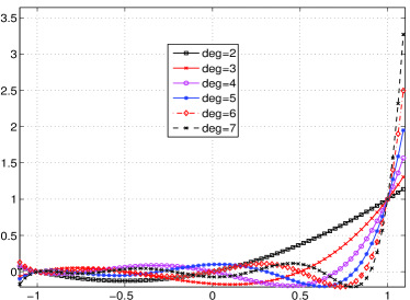
(a) Chebyshev interpolants of degrees 2 to 7

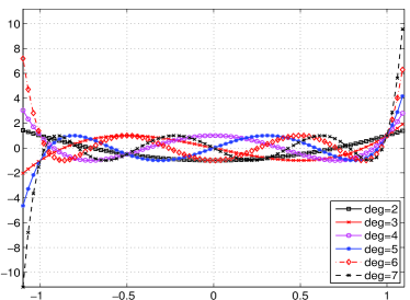
(b) Chebyshev polynomials of degrees 2 to 7

Fig. 1: illustration of polynomial functions

The idea of polynomial acceleration is straightforward and old, but its success is far from foolproof, largely due to inevitable errors in estimating intervals within which eigenvalues are supposed to be suppressed or promoted. The main reason for us to prefer our Chebyshev interpolates over the classic Chebyshev polynomials is that their lower profiles tend to make them less sensitive to erroneous intervals, hence easier to control. Indeed, our numerical comparison, albeit limited, appears to justify our choice.

6 Details of arrabit  Algorithms

In this section, we describe technical details and give parameter choices for our arrabit algorithm which computes $k$ eigenpairs corresponding to $k$ algebraically largest eigenvalues of a given symmetric matrix $A$.

Guard vectors. When computing $k$ eigenpairs, it is a common practice to compute a few extra eigenpairs to help guard against possible slow convergence. For this purpose, a small number of “guard vectors” are added to the iterate matrix $X$. In general, the more guard vectors are used, the less iterations are needed for convergence, but at a higher cost per iteration on memory and computing time. In our implementation, we set the number of columns in iterate matrix $X$ to $k+q$, where by default $q$ is set to $0.1k$ (rounded to the nearest integer).

Estimation of $\lambda_{n}$ and $\lambda_{k+q}$. To apply polynomial accelerators, we need to estimate the interval $[a,b]=[\lambda_{n},\lambda_{k+q}]$ which contains unwanted eigenvalues. The smallest eigenvalue $\lambda_{n}$ is computed by calling the the Matlab built-in solver eigs  (i.e., arpack [12]). Given an initial matrix $X\in\mathbb{R}^{n\times(k+q)}$ whose columns are orthogonalized, an under-estimation of $\lambda_{k+q}$ can be taken as the smallest eigenvalue of the projected matrix $X^{T}AX$ (which requires an RR projection). As the iterations progress, more accurate estimates of $\lambda_{k+q}$ will becomes available after each later ARR projection.

Outer loop stop rule. Let $(x_{i},\mu_{i})$, $i=1,2,\cdots,k$, be computed Ritz pairs where $x_{i}^{T}x_{j}=\delta_{ij}$. We terminate the algorithm when the following maximum relative residual norm becomes smaller than a prescribed tolerance $\mathrm{tol}$, i.e.,

(47) $$\mathtt{maxres}:=\max_{i=1,\ldots,k}\{\mathtt{res}_{i}\}\leq\mathrm{tol},$$

where

(48) $$\mathtt{res}_{i}:=\frac{\|Ax_{i}-\mu_{i}x_{i}\|_{2}}{\max(1,|\mu_{i}|)},\;i=1,\cdots,k.$$

The algorithm is also stopped in the following three cases: (i) if a maximum number of iterations, denoted by “maxit”, is reached (by default maxit = 30); or (ii) if the maximum relative residual norm has not been reduced after three consecutive outer iterations; or (iii) if most Ritz pairs have residuals considerably smaller than $\mathrm{tol}$ and the remaining have residuals slightly larger than $\mathrm{tol}$; specifically, $\mathtt{maxres}<(1+9h/k)\mathrm{tol}$ $(<10*\mathrm{tol})$, where $h$ is the number of Ritz pairs with residuals less than $0.1*\mathrm{tol}$. In our experiments we also monitor the computed partial trace $\sum_{i=1}^{k}\mu_{i}$ at the end for all solvers as a check for correctness.

Continuation. When a high accuracy (say, $\mathrm{tol}\leq 10^{-8}$) is requested, we use a continuation procedure to compute Ritz-pairs satisfying a sequence of tolerances: $\mathrm{tol}_{1}>\mathrm{tol}_{2}>\cdots\geq\mathrm{tol}$, and use the computed Ritz-pairs for $\mathrm{tol}_{t}$ as the starting point to compute the next solution for $\mathrm{tol}_{t+1}$. In our implementation, we use the update scheme

(49) $$\mathrm{tol}_{t+1}=\max(10^{-2}\,\mathrm{tol}_{t},\,\mathrm{tol}),$$

where $\mathrm{tol}_{1}$ is chosen to be considerably larger than $\mathrm{tol}$. A main reason for doing such a continuation is that our deflation procedure (see below) is tolerance-dependent. At the early stages of the algorithm, a stringent tolerance would delay the activation of deflation and likely cause missed opportunities in reducing computational costs.

Inner loop parameters and stop rule. Both mpm  and gn are tested as inner solvers to update $X$. These inner solvers are applied to the shifted matrix $A-aI$ which is supposedly positive semidefinite since $a$ is a good approximation to $\lambda_{n}$ (computed by eigs in our implementation). We check inner stopping criteria every $\mathrm{maxit}_{2}$ iterations and check them at most $\mathrm{maxit}_{1}$ times. In the present version, the default values for these two parameters are $\mathrm{maxit}_{1}=10$ and $\mathrm{maxit}_{2}=5$ Therefore, the maximum number of inner iterations allowed is $\mathrm{maxit}_{1}\times\mathrm{maxit}_{2}=50$.

The inner loop stopping criteria are either

(50) $$\mathtt{rc}=\mathtt{rcond}(X^{T}X)\leq\mathrm{tol}_{t}\mbox{\;\; or \; \; }\mathtt{rc}/\mathtt{rcp}>0.99,$$

where $\mathrm{tol}_{t}$ is the current tolerance (in a continuation sequence) and rcp is the previously computed $\mathrm{rcond}(X)$. In (50), we use the rcond subroutine in LAPACK (also used by Matlab) to estimate the reciprocal 1-norm condition number of $X^{T}X$, which we find to be relatively inexpensive. The first condition in (50) indicates that $X$ is about to lose (or have just lost) rank numerically, which implies that we achieve the goal of eliminating the unwanted eigenspace numerically. However, it is probable that a part of the desired eigenspace is also sacrificed, especially when there are clusters among the desired eigenvalues. Fortunately, this problem can be corrected, at a cost, in later iterations after deflation. On the other hand, the second condition is used to deal with the situation where the conditioning of $X$ does not deteriorate, which occurs from time to time in later iterations when there exists little or practically no decay in the relevant eigenvalues.

Deflation. Since Ritz pairs normally have uneven convergence rates, a procedure of detecting and setting aside Ritz pairs that have “converged” is called deflation or locking, which is regularly used in eigensolvers because it not only reduces the problem size but also facilitates the convergence of the remaining pairs. In our algorithm, a Ritz pair $(x_{i},\mu_{i})$ is considered to have “converged” with respect to a tolerance $\mathrm{tol}_{t}$ if its residual (see (48) for definition) satisfies

(51) $$\mathtt{res}_{i}\leq\max(10^{-14},\mathrm{tol}_{t}^{2}).$$

After each ARR projection, we collect the converged Ritz vectors into a matrix $Q_{c}$, and start the next iteration from those Ritz vectors “not yet converged”, which we continue to call $X$. Obviously, whenever $Q_{c}$ is nonempty $X$ is orthogonal to $Q_{c}$. Each time we check the stopping rule in the inner loop, we also perform a projection $X=X-Q_{c}(Q_{c}^{T}X)$ to ensure that $X$ stays orthogonal to $Q_{c}$. In addition, the next ARR projection will also be performed in the orthogonal complement of ${\cal{R}}(Q_{c})$. That is, we apply an ARR projection to the matrix $Y-Q_{c}(Q_{c}^{T}Y)$ for $Y=[X\;AZ\;\cdots\;A^{p}X]$. At the end, we always collect and keep $k+q$ leading Ritz pairs from both the “converged” and the “not yet converged” sets.

Augmentation blocks. The default value for the number of augmentation blocks is $p=1$, but this value may be adjusted after each ARR projection. We increase $p$ by one when we find that the relevant Ritz values show a small decay and at the same time the latest decrease in residuals is not particularly impressive. Specifically, we set $p=p+1$ if

(52) $$\frac{\mu_{k+q}}{\mu_{k}}>0.95\quad\mbox{ and }\quad\frac{\mathtt{maxres}}{\mathtt{maxresp}}>0.1,$$

where $\mathtt{maxresp}$ is the maximum relative residual norm at the previous iteration. The values $0.95$ and $0.1$ are set after some limited experimentation and by no means optimal. For $k$ relatively large, since the memory demand grows significantly as $p$ increases, we also limit the maximum value of $p$ to $p_{\max}=3$.

Polynomial degree. Under normal conditions, the higher degree is used in a polynomial accelerator, the fewer number of iterations will be required for convergence, but at a higher cost per iteration. A good balance is needed. Let $d$ and $d_{\max}$ be the initial and the largest polynomial degrees, respectively. We use the default values $d=3$ and $d_{\max}=15$. Let $\rho_{d}(t)$ be the polynomial function defined in (46). After each ARR step, we adjust the degree based on estimated spectral information of $\rho_{d}(A)$ computable using the current Ritz values. We know that the convergence rate of the inner solvers would be satisfactory if the eigenvalue ratio ${\rho_{d}(\lambda_{k+q})}/{\rho_{d}(\lambda_{k})}$ is small. Based on this consideration, we calculate

(53) $$\hat{d}=\min_{d\geq 3}\left\{d\in\mathbb{Z}:\frac{\rho_{d}(\mu_{k+q}^{*})}{\rho_{d}(\mu_{k}^{*})}<0.9\right\},$$

and then apply the cap $d_{\max}$ by setting

(54) $$d=\min(\hat{d},d_{\max})$$

where $\mu_{k}^{*}$ and $\mu_{k+q}^{*}$ are a pair of Ritz values corresponding to the iteration with the smallest residual “$\mathtt{maxres}$” defined in (47) (therefore the most accurate so far). The value of $0.9$ is of course adjustable.

Finally, a pseudocode for our arrabit  algorithm with all the above features is presented as Algorithm 8. This is the version used to produce the numerical results of this paper. As one can see, arrabit  algorithm uses $A$ only in matrix multiplications.

1 Input $A\in\mathbb{R}^{n\times n}$, integer $k\in(0,n)$ and tolerance $\mathrm{tol}>0$.

2 Choose $d$ and $d_{\max}$, the initial and maximum polynomial degrees. /* initialize */

3 Choose $p$ and $p_{\max}$, the initial and maximum number of augmentation blocks.

4 Choose $q\geq 0$, the number of guard vectors, so that $(p+1)(k+q)<n$.

5 Set tolerance parameters: $t=1$, $\mathrm{tol}_{t}\geq\mathrm{tol}$ and $\mathrm{tol}_{d}=\max(10^{-14},\mathrm{tol}_{t}^{2})$.

6 Initialize converged Ritz pairs $(Q_{c},\Sigma_{c})=\emptyset$ for deflation purposes.

7 Initialize an i.i.d. Gaussian random matrix $X\in\mathbb{R}^{n\times(k+q)}$.

8 Estimate the interval $[\lambda_{n},\lambda_{k+q}]\approx[a,b]$.

9 for $j=1,\ldots,\mathrm{maxit}$ do /* outer loop */

10       Initialize rc to infinity.

11      for $i_{1}=1,2,\cdots,\mathrm{maxit}_{1}$, do /* inner loop */

12             for $i_{2}=1,2,\cdots,\mathrm{maxit}_{2}$, do /* call inner solvers */

13                   if mpm  is the inner solver, then /* MPM */

14                         Call $X=\textsc{poly}(A-aI,X,0,b-a,\Gamma_{d})$. /* accelerator */

15                         Normalize the columns of $X$ individually.

16                  if gn  is the inner solver, then /* GN */

17                         Compute $Y=X\left(X^{T}X\right)^{-1}$.

18                         Call $Z=\textsc{poly}(A-aI,Y,0,b-a,\Gamma_{d})$. /* accelerator */

19                         Compute $X=Z-X(Y^{\mathrm{T}}Z-I)/2$.

20                  Compute $X=X-Q_{c}(Q_{c}^{T}X)$ if $Q_{c}\neq\emptyset$. /* projection */

21            Set $\mathrm{rcp}=\mathrm{rc}$ and compute $\mathrm{rc}=\mathrm{rcond}(X^{T}X)$.

22             if the inner stop rule (50) is met, then break.

23              /* end inner loop */

24      Compute $Y=[X,AX,\ldots,A^{p}X]$. /* augmentation */

25       $Y=Y-Q_{c}(Q_{c}^{T}Y)$ if $Q_{c}\neq\emptyset$. /* projection */

26       Perform ARR step: $(X,\Sigma)=\mathrm{RR}(A,Y)$. /* ARR */

27       Extract $k+q$ leading Ritz pairs $(x_{i},\mu_{i})$ from $(Q_{c},\Sigma_{c})$ and $(X,\Sigma)$.

28       Overwrite $(X,\Sigma)$ by the $k+q$ Ritz pairs. Compute residuals by (48).

29       if the outer stop rule (47) is met for $\mathrm{tol}$, then

30            output the Ritz pairs $(X,\Sigma)$ and exit. /* output and exit */

31            

32      if the outer stop rule (47) is met for $\mathrm{tol}_{t}$ then /* continuation */

33             Set $\mathrm{tol}_{t+1}=\max\left(10^{-2}\mathrm{tol}_{t},\mathrm{tol}\right)$, $b=\mu_{k+q}$ and $t=t+1$.

34      Collect converged Ritz pairs in $(Q_{c},\Sigma_{c})$ that satisfy (51). /* deflation */

35       Overwrite $(X,\Sigma)$ by the remaining not yet converged Ritz pairs.

36       if rules in (52) are met, then set $p=\min(p+1,p_{\max})$.

37        /* update p */ Update the polynomial degree by rules (53)-(54). /* update degree */

Algorithm 8 Algorithm arrabit (detailed version)

7 Numerical Results

In this section, we evaluate the performance of arrabit  on a set of sixteen sparse matrixes. Although we have constructed the algorithm with parallel scalability in mind as a major motivating factor, a study of scalability issues in a massively parallel environment is beyond the scope of the current paper.

As a first step, we test the algorithm in Matlab environment, on a single computing node (2 processors) and without explicit code parallelization, to determine how it performs in comparison to established solvers. We have implemented our arrabit algorithm, as is described by the pseudocode Algorithm 8, in MATLAB. For brevity, the two variants, corresponding to the two choices of inner solvers, will be called mpm  and gn, respectively.

We test two levels of accuracy in our experiments: $\mathrm{tol}=10^{-6}$ or $\mathrm{tol}=10^{-12}$. By our stoping rule, upon successful termination the largest eigenpair residual will not exceed $10^{-5}$ or $10^{-11}$, respectively. Since our algorithm checks the termination rule only after each ARR call, it often returns solutions of higher accuracies than what is prescribed by the $\mathrm{tol}$ value.

7.1 Solvers, Platform and Test Matrices

Since it is impractical to carry out numerical experiments with a large number of solvers, we have carefully chosen two high-quality packages to compare with our arrabit code. One package is arpack [12], which is behind the Matlab built-in iterative eigensolver eigs, and will naturally serve as the benchmark solver. Another is a more recent package called feast [28] which has been integrated into Intel’s Math Kernel Library (MKL) under the name “Intel MKL Extended Eigensolver”. Both arpack  and feast  are written in Fortran. While arpack  can be directly accessed through eigs  in Matlab, we call feast  from Intel’s MKL Library via Matlab’s MEX external interfaces. In our experiments, all parameters in eigs  and feast  are set to their default values, and each solver terminates with its own stopping rules using either $\mathrm{tol}=10^{-6}$ or $\mathrm{tol}=10^{-12}$.

We have also examined a few other solvers as potential candidates but decided not to use them in this paper, including but not limited to the filtered Lanczos algorithm [6] and the Chebyshev-Davidson algorithm [29]. Our initial tests indicated that, for various reasons, these solvers’ overall performance could not measure up with that of the commercial-grade software packages arpack  and feast on a number of test problems. This fact may be more of a reflection on the current status of software development for these solvers than on the merits of the algorithms behind.

It is important to note that feast  is designed to compute all eigenvalues (and their eigenvectors) in an interval, which is given as an input along with an estimated number of eigenvalues inside the interval. When computing $k$ largest eigenpairs, we have observed that the performance of feast  is affected greatly by the quality of the two estimations: the interval itself and the number of eigenvalues inside the interval. When calling feast, we set (i) the interval to be $[\lambda_{k}^{*},\lambda_{1}^{*}]$ where $\lambda_{k}^{*}$ and $\lambda_{1}^{*}$ are computed eigenvalues by eigs  using the same tolerance $\mathrm{tol}$; and (ii) the estimated number of eigenvalues in the interval to $1.2k$ rounded to the nearest integer. We consider this setting to be fair, if not overly favorable, to feast.

Our numerical experiments are preformed on a single computing node of Edison, a Cray XC30 supercomputer maintained at the National Energy Research Scientific Computer Center (NERSC) in Berkeley. The node consists of two twelve-core Intel “Ivy Bridge” processors at 2.4 GHz with a total of 64 GB shared memory. Each core has its own L1 and L2 caches of 64 KB and 256 KB, respectively; A 30-MB L3 cache shared between 12 cores on the “Ivy Bridge” processor. We generate Matlab standalone executable programs and submit them as batch jobs to Edison. The reported runtimes are wall-clock times.

On a multi/many-core computer, memory access patterns and communication overheads have a notable impact on computing time. In Matlab, dense linear algebra operations are generally well optimized by using BLAS and LAPACK tuned to the CPU processors in use. On the other hand, we have observed that some sparse linear algebra operations in Matlab seem to have not been as highly optimized (at least in version 2013b). In particular, when doing multiplications between a large sparse matrix and a dense matrix (like $AX$), Matlab is often slower than a routine in Intel’s Math Kernel Library (MKL) named “mkl_dcscmm” when it is invoked through Matlab’s MEX external interfaces in our experiments. For this reason, we use this MKL routine in our Matlab code to perform the operation $AX$.

Our test matrices are selected from the University of Florida Sparse Matrix Collection. For each matrix, we compute both $k$ eigenpairs corresponding to $k$ largest eigenvalues and those corresponding to $k$ smallest eigenvalues. Many of the selected matrices are produced by PARSEC [8], a real space density functional theory (DFT) based code for electronic structure calculation in which the Hamiltonian is discretized by a finite difference method. We do not take into account any background information for these matrices; instead, we simply treat them algebraically as matrices.

Table 1 lists, for each matrix $A$, the dimensionality $n$, the number of nonzeros $nnz(A)$ and the density of $A$, i.e., the ratio $({nnz(A)}/{n^{2}})100\%$. The number of eigenpairs to be computed is set either to 1% of $n$ rounded to the nearest integer or to $k=1000$ whichever is smaller. Table 1 also reports the number of the nonzeros in the Cholesky factor $L$ of matrix $A-\alpha I$ where $\alpha=\max(2\lambda_{n}(A),0)$. The factorization is carried out after an “approximate minimum degree” permutation performed by the Matlab function “amd”, as is done by the following MATLAB line: $\mathtt{t=amd(B);~{}L=chol(B(t,t),^{\prime}lower^{\prime})}.$ We have also tested the “symmetric approximate minimum degree” permutation (“symamd” in Matlab), but the corresponding density of $L$ is slightly larger on most matrices. The density of factor $L$ and the computing time in seconds used by Cholesky factorization are also given in Table 1. Although all matrices $A$ are very sparse, the Cholesky factors of some matrices, such as Ga10As10H30, Ga3As3H12 and Ge87H76, are quite dense. As a result, the Cholesky factorization time varies greatly from matrix to matrix. We mention that the spectral distributions of the test matrices can behave quite differently from matrix to matrix. Even for the same matrix, the spectrum of a matrix can change behavior drastically from region to region. Most notably, computing $k$ smallest eigenpairs of many matrices in this set turns out to be more difficult than computing $k$ largest ones.

The largest matrix size in this set is more than a quarter of million. Relative to the computing resources in use, we consider these selected matrices to be fairly large scale. Overall, we consider this test set reasonably diverse and representative, fully aware that there always exist instances out there that are more challenging to one solver or another.

Table 1: Information of Test Matrices

matrix name	$n$	$k$	$nnz(A)$	density of A	nnz(L)	density of L	time
Andrews	60000	600	760154	0.021%	117039940	6.502%	7.18
C60	17576	176	407204	0.132%	34144169	22.105%	1.62
cfd1	70656	707	1825580	0.037%	35877440	1.437%	1.81
finance	74752	748	596992	0.011%	2837714	0.102%	0.28
Ga10As10H30	113081	1000	6115633	0.048%	1562547805	24.439%	127.12
Ga3As3H12	61349	613	5970947	0.159%	596645077	31.705%	42.00
shallow_water1s	81920	819	327680	0.005%	2357535	0.070%	0.21
Si10H16	17077	171	875923	0.300%	56103003	38.474%	2.60
Si5H12	19896	199	738598	0.187%	78918573	39.871%	3.80
SiO	33401	334	1317655	0.118%	186085449	33.359%	10.01
wathen100	30401	304	471601	0.051%	1490209	0.322%	0.32
Ge87H76	112985	1000	7892195	0.062%	1403571238	21.990%	109.64
Ge99H100	112985	1000	8451395	0.066%	1477089634	23.141%	120.08
Si41Ge41H72	185639	1000	15011265	0.044%	3457063398	20.063%	358.53
Si87H76	240369	1000	10661631	0.018%	5568995364	19.277%	1499.80
Ga41As41H72	268096	1000	18488476	0.026%	6998257446	19.473%	2498.43

7.2 Comparison between RR and ARR

We first evaluate the performance difference between ARR and RR for both mpm  and gn. Table 7.2 gives results for computing both $k$ largest and smallest eigenpairs on the first six matrices in Table 1 to the accuracy of $\mathrm{tol}=10^{-12}$. We note that RR and ARR correspond to $p=0$ and $p>0$, respectively, in Algorithm 8. In order to differentiate the effect of changing $p$ from that of changing the polynomial degree, we also test a variant of Algorithm 8 with a fixed polynomial degree at $d=8$ (by skipping line 34). In Table 7.2, “$\mathtt{maxres}$” denotes the maximum relative residual norm in (47), “time” is the runtime measured in seconds, “RR” is the total number of the outer iterations, i.e., the total number of the RR or ARR calls made (excluding the one called in preprocessing for estimating $\lambda_{k+q}$), and “$p$” and “$d$” are the number of augmentation blocks and the polynomial degree, respectively, used at the final outer iteration. In addition, on the matrices cfd1 and finance we plot the (outer) iteration history of $\mathtt{maxres}$ in Figures 3 and 3 for computing $k$ largest and smallest eigenpairs, respectively.

The following observations can be drawn from the table and figures.

• The performances of mpm  and gn  are similar. For both of them, ARR can accelerate convergence, reduce the number of outer iterations needed, and improve the accuracy, often to a great extent.

• The scheme of adaptive polynomial degree generally works better than a fixed polynomial degree. A more detailed look at the effect of polynomial degrees is presented in Section 7.3.

• The default value $p=1$ for the number of augmentation blocks in ARR is generally kept unchanged (recall that it can be increased by the algorithm).

• The total number of ARR called is mostly very small, especially in the cases where the adaptive polynomial degree scheme is used and the $k$ largest eigenpairs are computed (which tend to be easier than the $k$ smallest ones). We observe from Figure 3 that in several cases a single ARR is sufficient to reach the accuracy of $\mathrm{tol}$=1e-6 (even of $\mathrm{tol}$=1e-12 in one case).

Table 2: Comparison results between RR and ARR with tol=1e-12

	mpm  with RR					mpm  with ARR					gn  with RR					gn  with ARR
matrix	maxres	time	RR	p/d		maxres	time	RR	p/d		maxres	time	RR	p/d		maxres	time	RR	p/d
computing k largest eigpair by fix deg = 8
Andrew.	9.5e-13	191	4	1/ 8		1.9e-06	250	9	3/ 8		9.0e-12	174	6	1/ 8		9.9e-13	104	2	1/ 8
C60	4.0e-12	45	11	3/ 8		6.3e-12	12	3	1/ 8		7.5e-12	44	22	3/ 8		1.4e-12	16	5	1/ 8
cfd1	9.8e-13	381	4	1/ 8		1.0e-12	296	4	1/ 8		9.8e-13	294	4	1/ 8		9.9e-13	206	2	1/ 8
financ.	9.9e-13	157	3	1/ 8		8.9e-13	151	3	1/ 8		1.0e-12	196	4	1/ 8		1.0e-12	141	2	1/ 8
Ga10As.	3.5e-13	1218	22	3/ 8		9.9e-13	1483	8	2/ 8		6.1e-12	910	8	1/ 8		9.9e-13	448	3	1/ 8
Ga3As3.	9.7e-13	467	6	1/ 8		9.8e-13	270	5	1/ 8		1.9e-12	307	8	1/ 8		9.4e-13	179	3	1/ 8
computing k largest eigpair with adaptive polynomial degree
Andrew.	2.0e-11	337	9	3/ 5		8.8e-13	148	5	2/ 5		5.3e-12	319	17	3/ 5		1.0e-12	125	4	1/ 5
C60	8.7e-12	41	10	3/ 9		2.0e-12	13	3	1/ 9		4.2e-12	42	20	3/ 9		5.5e-12	13	3	1/ 9
cfd1	1.3e-12	441	5	1/ 3		9.8e-13	190	4	1/ 3		4.1e-12	482	17	3/ 3		9.9e-13	188	3	1/ 3
financ.	9.9e-13	256	4	1/ 3		1.3e-12	97	3	2/ 3		2.7e-12	380	14	3/ 3		1.1e-12	69	1	1/ 3
Ga10As.	4.7e-12	1199	6	1/ 5		9.6e-13	442	4	1/ 5		7.1e-12	1442	19	3/ 5		9.7e-13	580	4	1/ 6
Ga3As3.	2.9e-12	473	7	2/ 5		1.7e-12	169	4	1/ 5		3.9e-12	494	17	3/ 5		1.7e-12	198	4	1/ 5
computing k smallest eigpair by fix deg = 8
Andrew.	4.2e-12	465	7	2/ 8		1.5e-13	219	6	2/ 8		7.2e-12	475	19	3/ 8		1.0e-12	199	5	1/ 8
C60	1.7e-12	30	9	3/ 8		6.8e-13	17	6	1/ 8		5.5e-12	24	13	3/ 8		6.7e-12	13	4	1/ 8
cfd1	4.1e-05	2870	30	3/ 8		6.0e-12	1543	21	3/ 8		1.5e-04	2505	30	3/ 8		7.9e-12	1394	22	3/ 8
financ.	3.8e-08	1759	30	3/ 8		5.1e-13	700	9	3/ 8		3.5e-06	1651	30	3/ 8		7.2e-13	713	11	3/ 8
Ga10As.	8.6e-10	2642	10	3/ 8		3.7e-12	1372	5	1/ 8		2.1e-02	1436	6	1/ 8		2.6e-12	961	4	1/ 8
Ga3As3.	7.2e-12	964	11	3/ 8		2.7e-12	489	4	1/ 8		4.2e-12	994	24	3/ 8		9.9e-13	381	4	1/ 8
computing k smallest eigpair with adaptive polynomial degree
Andrew.	7.3e-12	466	8	3/ 8		9.7e-13	200	4	1/ 8		8.9e-12	505	21	3/ 8		1.1e-12	185	5	1/ 8
C60	6.7e-12	38	9	3/ 7		2.8e-12	26	9	3/ 6		4.0e-12	31	23	3/ 6		9.2e-13	15	8	2/ 6
cfd1	3.7e-08	2869	30	3/15		8.9e-12	719	4	1/15		2.3e-06	2515	30	3/15		4.2e-12	1017	12	3/15
financ.	3.7e-12	1391	9	3/15		1.4e-12	600	6	1/15		5.3e-12	1416	24	3/15		3.4e-12	467	5	1/15
Ga10As.	4.5e-11	3261	12	3/ 8		1.1e-12	1558	6	1/ 8		2.9e-12	3681	24	3/ 8		4.0e-12	963	3	1/ 9
Ga3As3.	5.9e-12	1046	8	3/ 9		9.9e-13	420	4	1/ 9		7.7e-12	1238	24	3/ 9		9.5e-13	338	5	1/ 9

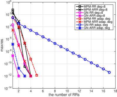
(a) matrix: cfd1

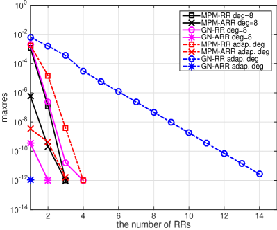
(b) matrix: finance

Fig. 2: ARR vs RR: Iteration history of $\mathtt{maxres}$ for computing $k$ largest eigenpairs

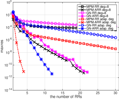
(a) matrix: cfd1

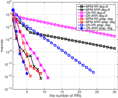
(b) matrix: finance

Fig. 3: ARR vs RR: Iteration history of $\mathtt{maxres}$ for computing $k$ smallest eigenpairs

7.3 Comparison on Polynomials

We next examine the effect of polynomial degrees on the convergence behavior of mpm  and gn, again on the first six matrices in Table 1. We compare two schemes: the first is to use a fix degree among $\{4,8,15\}$ and skip line 34 of Algorithm 8, and the second is the adaptive scheme in Algorithm 8. The computational results are summarized in Table 7.3. We also plot the iteration history of $\mathtt{maxres}$, for computing both $k$ largest and smallest eigenpairs on the matrices cfd1 and finance in Figures 5 and 5, respectively. The numerical results lead to the following observations:

• Again the performances of mpm  and gn  are similar, and the default value $p=1$ for augmentation is mostly unchanged.

• In general, the number of outer iterations is decreased as the polynomial degree is increased, but the runtime time is not necessarily reduced because of the extra cost in using higher-degree polynomials. Overall, our adaptive strategy seems to have achieved a reasonable balance.

• With fixed polynomial degrees, in a small number of test case mpm  and gn  fail to reach the required accuracy.

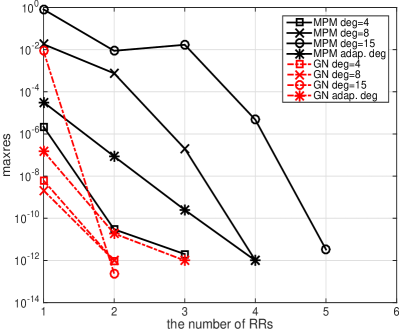
(a) matrix: cfd1

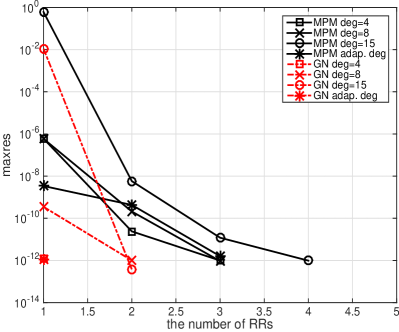
(b) matrix: finance

Fig. 4: ARR: Iteration history of $\mathtt{maxres}$ for computing $k$ largest eigenpairs using different polynomial degrees

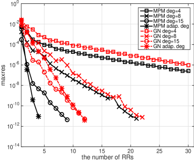
(a) matrix: cfd1

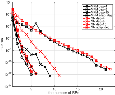
(b) matrix: finance

Fig. 5: ARR: Iteration history of $\mathtt{maxres}$ for computing $k$ smallest eigenpairs using different polynomial degrees

Table 3: Comparison results of different polynomial degrees on tol=1e-12

Finally, we compare the performance of Algorithm 8 either using Chebyshev interpolates defined in (45) or the Chebyshev polynomials defined in (7) on the first six matrices in Table 1. The comparison results are given in Table  7.3. Even though both types of polynomials work well on these six problems, some performance differences are still observable in favor of our polynomials.

Table 4: Comparison results on Chebyshev interpolates in (45) and Chebyshev polynomials in (7)

7.4 Comparison with arpack and feast

We now compare mpm  and gn  with eigs  and feast  for computing both $k$ largest and smallest eigenpairs for all sixteen test matrices presented in Tables 1 (which also lists the $k$ values). Computational results are summarized in Tables 7.4 and 7.4, where “SpMV” denotes the total number of SpMVs, counting each operation $AX\in\mathbb{R}^{n\times k}$ as $k$ SpMVs.

In addition, the speedup with respect to the benchmark time of eigs  is measured by the quantity $\log_{2}(\mathrm{time}_{\textsc{eigs}}/\mathrm{time})$, as shown in Figures 7 and 7 where a positive bar represents a “speedup” and a negative one a “slowdown”. In these two figures, matrices are ordered from left to right in ascending order of the solution time used by eigs; that is, when moving from the left towards the right, problems become progressively more and more time-consuming for eigs  to solve. A quick glance at the figures tells us that mpm and gn  provide clear speedups over eigs  on most problems, especially on the more time-consuming problems towards the right. For example, mpm and gn  deliver a speedup of about 4 times on each of the seven most time-consuming problems in Figure 7(a), and a speedup of about 10 times on the most time-consuming problem Ga41As41H72 in Figure 7(a). On the other hand, compared to eigs, feast’s timing profile looks volatile with both big “speedups” and “slowdowns”.

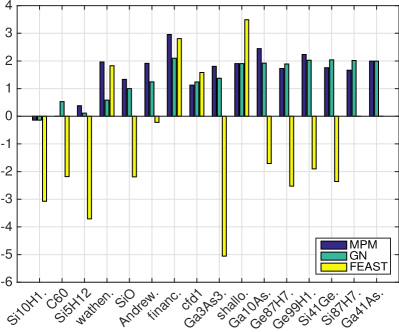
(a) $\mathrm{tol}=10^{-6}$

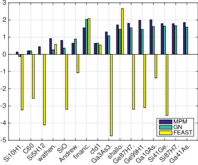
(b) $\mathrm{tol}=10^{-12}$

Fig. 6: Speedup to eigs: $\log_{2}(\mathrm{time}_{\textsc{eigs}}/\mathrm{time})$ on computing $k$ largest eigenpairs

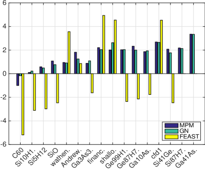
(a) $\mathrm{tol}=10^{-6}$

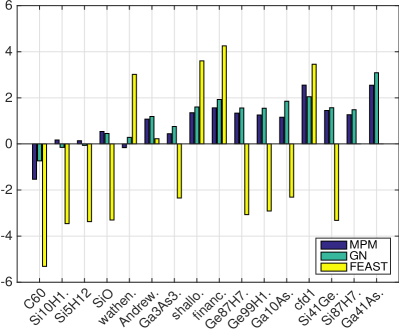
(b) $\mathrm{tol}=10^{-12}$

Fig. 7: Speedup to eigs: $\log_{2}(\mathrm{time}_{\textsc{eigs}}/\mathrm{time})$ on computing $k$ smallest eigenpairs

Table 5: Comparison results on computing $k$ largest eigenpairs

Table 6: Comparison results on computing $k$ smallest eigenpairs

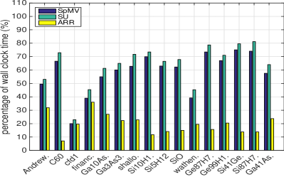
(a) $\mathrm{tol}=10^{-6}$, mpm, k largest eigenpairs

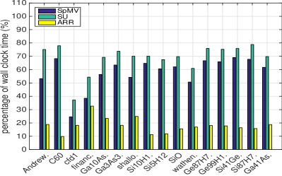
(b) $\mathrm{tol}=10^{-12}$, mpm, k largest eigenpairs

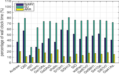
(c) $\mathrm{tol}=10^{-6}$, gn, k largest eigenpairs

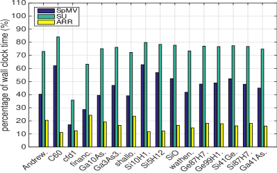
(d) $\mathrm{tol}=10^{-12}$, gn, k largest eigenpairs

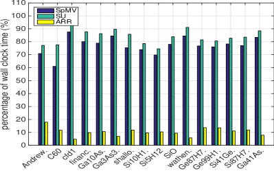
(e) $\mathrm{tol}=10^{-6}$, mpm, k smallest eigenpairs

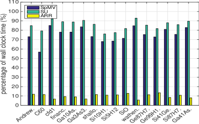
(f) $\mathrm{tol}=10^{-12}$, mpm, k smallest eigenpairs

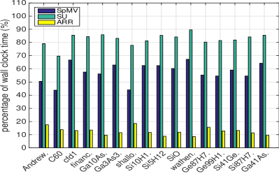
(g) $\mathrm{tol}=10^{-6}$, gn, k smallest eigenpairs

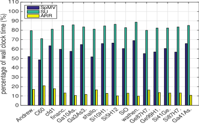
(h) $\mathrm{tol}=10^{-12}$, gn, k smallest eigenpairs

Fig. 8: A comparison of timing profile among SpMV, SU and ARR

The benchmark solver eigs  usually, though not always, returns solutions more accurate than what is requested by the tolerance value. In particular, for $\mathrm{tol}=10^{-6}$ the accuracy of eigs  solutions often reach the order of $O(10^{-12})$. This is due to the fact that eigs  need to maintain a high working accuracy to ensure proper convergence.

As is observed previously, it is often more time-consuming for eigs, mpm  and gn  to compute $k$ smallest eigenpairs than $k$ largest ones on many test matrices. By examining the spectra of the matrices such as cfd1 and finance, we believe that this phenomenon is attributable to the property that these matrices tend to have a flatter end on the left end of their spectra. On the other hand, the behavior of feast  appears less affected by this property but more by sparsity patterns (see below).

Concerning the performance of feast, we make the following observations.

• feast  solves most problems successfully but fails to correctly solve a few cases. When computing $k$ largest eigenvalues for the matrix Ga10As10H30 feast  returns the warning: “No eigenvalue has been found in the proposed search interval”. On matrix Ga3As3H12, it seems to exit normally with the output messages “Eigensolvers have successfully converged”, but the subsequently computed maximum relative residual norm in (47) is way too large at $0.29$. On matrices Ga41As41H72 and Si87H76, when computing either $k$ largest or smallest eigenpairs, feast  terminates abnormally after spending a long computing time, with the message: “Eigensolvers ERROR: Problem from Inner Linear System Solver”. By examining the density of Cholesky factors for Ga41As41H72 and Si87H76 in Table 1, we speculate that the abnormal termination most likely has to do with excessive memory demands encountered by the inner linear system solver in Intel Math Kernel Library.

• For $\mathrm{tol}=10^{-12}$, feast  is the fastest in solving finance and shallow_water1s for $k$ largest eigenpairs, and in solving cfd1, finance, shallow_water1s and wathen100 for $k$ smallest eigenpairs. On the other hand, feast  can be significantly slower than others on matrices such as Ga10As10H30, Ga3As3H12, Ge87H76, Ge99H100, Si41Ge41H72, Si87H76 and Ga41As41H72. The performance of feast  can be at least partly explained from the density of Cholesky factors $L$ shown in Table 1, since feast  uses a direct linear solver in Intel Math Kernel Library to compute factorizations of matrices of the form $(\phi_{l}I-A)$ in (8). We can clearly see the correlation that feast  is fast when the density of the Cholesky factor is low and Cholesky factorization is fast.

With regard to the performance of mpm  and gn, we make the following observations.

• mpm  and gn  both attain the required accuracy on all test problems, and they often return smaller residual errors than what is required by $\mathrm{tol}$. Generally speaking, the two variants perform quite similarly in terms of both accuracy and timing.

• mpm  and gn  maintain a clear speed advantage over feast  in most tested cases. They are faster than feast  when either factorizations of shifted $A$ are expensive, or when spectral distributions have a favorable decay (for example, on cfd1 for computing $k$ largest eigenpairs).

• mpm  and gn  also maintain an overall speed advantage over eigs, especially on those problems more time-consuming for eigs  (towards the right end of Figures 7 and 7). They are faster in spite of taking considerably more matrix-vector multiplications than eigs, as can be seen from Tables 7.4 and 7.4, thanks to the benefits of relying on high-concurrency operations on many-core computers.

• mpm  and gn  generally require a smaller number ARR calls, often only two or three when computing $k$ largest eigenpairs. In quite a number of cases (for example, on finance and wathen100 for mpm and so on), only a single ARR projection is taken which is absolutely optimal in order to extract approximate eigenpairs.

• The number of augmentation blocks used by mpm  and gn  is usually $1$, and the final polynomial degree never reaches the maximum degree $15$ except on cfd1, finance and wathen100 when computing $k$ smallest eigenpairs.

In Figure 8, we plot runtimes of three categories: SpMV (i.e., $AX$), SU (lines 10 to 22 of Algorithm 8) and ARR (lines 23 to 27 of Algorithm 8). In particular, SpMVs are called in both SU and ARR, but overwhelmingly in the former. These are the major computational components of mpm  and gn. The runtime of each category is measured in the percentage of wall-clock time spent in that category over the total wall-clock time. We can see, especially from the time-consuming problems on the right, that (i) the time of SU dominates that of RR, and (ii) the time of SpMVs, always done in batch of $k+q$, dominates the entire computation in almost all cases. These trends are much more pronounced (a) for mpm  than for gn  (recall that gn  requires to solve $k\times k$ linear systems); and (b) for computing $k$ smallest eigenpairs than for computing $k$ largest ones (recall that the former is generally more difficult). These runtime profiles are favorable to parallel scalability since $AX$ operations possess high concurrency for relatively large $k$.

In the final set of experiments, we examine the solvers’ scalability with respect to $k$. We apply the solvers to matrices cfd1 and Ge87H76, with $\mathrm{tol}=10^{-12}$, and vary $k$ from $100,200$ up to $1200$ with increment $200$ (there are exceptions for feast). The resulting solution times are plotted in Figures 10 and 10. In both figures, the slopes of the time curves confirm that the three block algorithms, feast, mpm  and gn, clearly scale better with respect to $k$ than the Krylov subspace algorithm eigs. Although eigs can be the fastest for $k$ small, its solution time increases at a faster pace than the block methods as $k$ increases.

Among the block algorithms themselves, all three provide comparable performances on cfd1 when computing the $k$ largest eigenpairs, while feast  is the fastest when computing $k$ smallest eigenpairs. On Ge87H76, which has a rather dense Cholesky factor, feast  is much slower in all runs up to $k=1000$ (runs for $k>1000$ are skipped to save time).

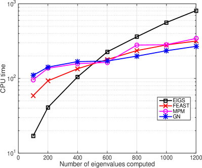
(a) $k$ largest eigenpairs, $tol=10^{-12}$

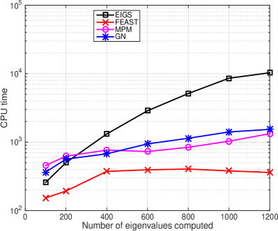
(b) $k$ smallest eigenpairs, $tol=10^{-12}$

Fig. 9: Comparison results of solution time for computing $k$ eigenpairs of the matrix cfd1

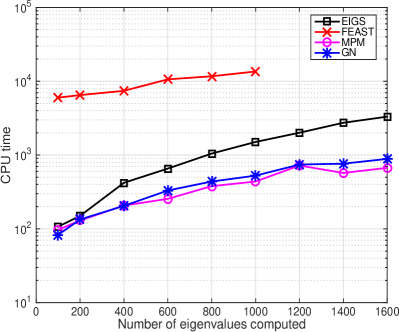
(a) $k$ largest eigenpairs, $tol=10^{-12}$

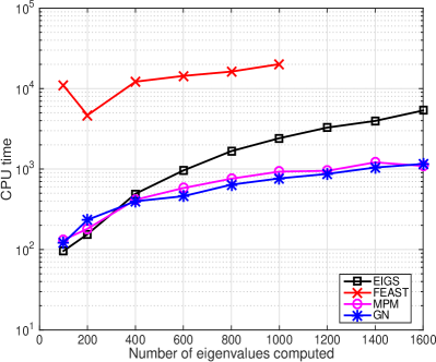
(b) $k$ smallest eigenpairs, $tol=10^{-12}$

Fig. 10: Comparison results on solution time for computing $k$ eigenpairs of the matrix Ge87H76.

8 Concluding Remarks

The goal of this paper is to construct a block algorithm of high scalability suitable for computing relatively large numbers of exterior eigenpairs for really large-scale matrices on modern computers. Our strategy is simple: to reduce as much as possible the number of RR calls (Rayleigh-Ritz projections) or, in other words, to shift as much as possible computation burdens to SU (subspace update) steps. This strategy is based on the following considerations. RR steps perform small dense eigenvalue decompositions, as well as basis orthogonalizations, thus possessing limited concurrency. On the other hand, SU steps can be accomplished by block operations like $A$ times $X$, thus more scalable.

To reach for maximal concurrency, we choose the power iteration for subspace updating (and also include a Gauss-Newton method to test the versatility of our construction). It is well known that the convergence of the power method can be intolerably slow, preventing it from being used to drive general-purpose eigensolvers. Therefore, the key to success reduces to whether we could accelerate the power method sufficiently and reliably to an extent that it can compete in speed with Krylov subspace methods in general. In this work, such an acceleration is accomplished mainly through the use of three techniques: (1) an augmented Rayleigh-Ritz (ARR) procedure that can provably accelerate convergence under mild conditions; (2) a set of easy-to-control, low-degree polynomial accelerators; and (3) a bold stoping rule for SU steps that essentially allows an iterate matrix to become numerically rank-deficient. Of course, the success of our construction also depends greatly on a set of carefully integrated algorithmic details. The resulting algorithm is named arrabit, which uses $A$ only in matrix multiplications.

Numerical experiments in Matlab on sixteen test matrices from the UF Sparse Matrix Collection show, convincingly in our view, that the accuracy and efficiency of arrabit  is indeed competitive to start-of-the-art eigensolvers. Exceeding our expectations, arrabit  can already provide multi-fold speedups over the benchmark solver eigs, without explicit code parallelization and without running on massively parallel machines, on difficult problems. In particular, it often only needs two or three, sometimes just one, ARR projections to reach a good solution accuracy.

There are a number of future directions worth pursuing from this point on. For one thing, the robustness and efficiency of arrabit can be further enhanced by refining its construction and and tuning its parameters. Software development and an evaluation of its parallel scalability are certainly important. The prospective of extending the algorithm to non-Hermitian matrices and the generalized eigenvalue problem looks promising. Overall, we feel that the present work has laid a solid foundation for these and other future activities.

Acknowledgements

Most of the computational results were obtained at the National Energy Research Scientific Computing Center (NERSC), which is supported by the Director, Office of Advanced Scientific Computing Research of the U.S. Department of Energy under contract number DE-AC02-05CH11232.

References

- [1] Z. Bai, J. Demmel, J. Dongarra, A. Ruhe, and H. van der Vorst, Templates for the Solution of Algebraic Eigenvalue Problems: A Practical Guide, Society for Industrial and Applied Mathematics, Philadelphia, PA, USA, 2000.
- [2] M. Bollhöfer and Y. Notay, JADAMILU: a software code for computing selected eigenvalues of large sparse symmetric matrices, Comput. Phys. Comm., 177 (2007), pp. 951–964.
- [3] J. W. Demmel, Applied Numerical Linear Algebra, Society for Industrial and Applied Mathematics, Philadelphia, PA, USA, 1997.
- [4] T. A. Driscoll, N. Hale, and L. N. Trefethen, Chebfun Guide, Pafnuty Publications, 2014.
- [5] H. Ehlich and K. Zeller, Auswertung der normen von interpolationsoperatoren, Mathematische Annalen, 164 (1966), pp. 105–112.
- [6] H.-R. Fang and Y. Saad, A filtered Lanczos procedure for extreme and interior eigenvalue problems, SIAM J. Sci. Comput., 34 (2012), pp. A2220–A2246.
- [7] A. V. Knyazev, Toward the optimal preconditioned eigensolver: locally optimal block preconditioned conjugate gradient method, SIAM J. Sci. Comput., 23 (2001), pp. 517–541.
- [8] L. Kronik, A. Makmal, M. Tiago, M. M. G. Alemany, X. Huang, Y. Saad, and J. R. Chelikowsky, PARSEC – the pseudopotential algorithm for real-space electronic structure calculations: recent advances and novel applications to nanostructures, Phys. Stat. Solidi. (b), 243 (2006), pp. 1063–1079.
- [9] C. Lanczos, An iteration method for the solution of the eigenvalue problem of linear differential and integral operators, J. Res. Nat’l Bur. Std., 45 (1950), pp. 225–282.
- [10] R. M. Larsen, Lanczos bidiagonalization with partial reorthogonalization, Aarhus University, Technical report, DAIMI PB-357, September 1998.
- [11] R. B. Lehoucq, Implicitly restarted Arnoldi methods and subspace iteration, SIAM J. Matrix Anal. Appl., 23 (2001), pp. 551–562.
- [12] R. B. Lehoucq, D. C. Sorensen, and C. Yang, ARPACK users’ guide: Solution of large-scale eigenvalue problems with implicitly restarted Arnoldi methods, vol. 6 of Software, Environments, and Tools, Society for Industrial and Applied Mathematics (SIAM), Philadelphia, PA, 1998.
- [13] X. Liu, Z. Wen, and Y. Zhang, Limited memory block krylov subspace optimization for computing dominant singular value decompositions, SIAM Journal on Scientific Computing, 35-3 (2013), pp. A1641–A1668.
- [14] X. Liu, Z. Wen, and Y. Zhang, An efficient Gauss-Newton algorithm for symmetric low-rank product matrix approximations, SIAM Journal on Optimization, (To appear 2015).
- [15] G. Mastroianni and J. Szabados, Jackson order of approximation by lagrange interpolation. ii, Acta Mathematica Hungarica, 69 (1995), pp. 73–82.
- [16] B. Parlett, The Symmetric Eigenvalue Problem, Prentice-Hall, 1980.
- [17] E. Polizzi, Density-matrix-based algorithm for solving eigenvalue problems, Phys. Rev. B, 79 (2009), p. 115112.
- [18] H. Rutishauser, Computational aspects of F. L. Bauer’s simultaneous iteration method, Numer. Math., 13 (1969), pp. 4–13.
- [19] H. Rutishauser, Simultaneous iteration method for symmetric matrices, Numer. Math., 16 (1970), pp. 205–223.
- [20] Y. Saad, Chebyshev acceleration techniques for solving nonsymmetric eigenvalue problems, Mathematics of Computation, 42 (1984), pp. 567–588.
- [21] Y. Saad, Numerical Methods for Large Eigenvalue Problems, Manchester University Press, 1992.
- [22] A. H. Sameh and J. A. Wisniewski, A trace minimization algorithm for the generalized eigenvalue problem, SIAM Journal on Numerical Analysis, 19 (1982), pp. pp. 1243–1259.
- [23] D. C. Sorensen, Implicitly restarted Arnoldi/Lanczos methods for large scale eigenvalue calculations, in Parallel numerical algorithms (Hampton, VA, 1994), vol. 4 of ICASE/LaRC Interdiscip. Ser. Sci. Eng., Kluwer Acad. Publ., 1996, pp. 119–165.
- [24] A. Stathopoulos and C. F. Fischer, A davidson program for finding a few selected extreme eigenpairs of a large, sparse, real, symmetric matrix, Computer Physics Communications, 79 (1994), pp. 268–290.
- [25] G. W. Stewart, Simultaneous iteration for computing invariant subspaces of non-Hermitian matrices, Numer. Math., 25 (1975/76), pp. 123–136.
- [26] , Matrix algorithms Vol. II: Eigensystems, Society for Industrial and Applied Mathematics (SIAM), Philadelphia, PA, 2001.
- [27] W. J. Stewart and A. Jennings, A simultaneous iteration algorithm for real matrices, ACM Trans. Math. Software, 7 (1981), pp. 184–198.
- [28] P. T. P. Tang and E. Polizzi, FEAST as a subspace iteration eigensolver accelerated by approximate spectral projection, SIAM J. Matrix Anal. Appl., 35 (2014), pp. 354–390.
- [29] Y. Zhou and Y. Saad, A Chebyshev–Davidson algorithm for large symmetric eigenproblems, SIAM J. Matrix Anal. and Appl., 29 (2007), pp. 954–971.