X-RAY AND RADIO EMISSION FROM TYPE IIn SUPERNOVA SN 2010jl

Abstract

We present all X-ray and radio observations of the Type IIn supernova SN 2010jl. The X-ray observations cover a period up to day 1500 with Chandra , XMM-Newton , NuSTAR , and Swift-XRT . The Chandra observations after 2012 June, the XMM-Newton observation in 2013 November, and most of the Swift-XRT observations until 2014 December are presented for the first time. All the spectra can be fitted by an absorbed hot thermal model except for Chandra spectra on 2011 October and 2012 June when an additional component is needed. Although the origin of this component is uncertain, it is spatially coincident with the supernova and occurs when there are changes to the supernova spectrum in the energy range close to that of the extra component, indicating that the emission is related to the supernova. The X-ray light curve shows an initial plateau followed by a steep drop starting at day $\sim 300$. We attribute the drop to a decrease in the circumstellar density. The column density to the X-ray emission drops rapidly with time, showing that the absorption is in the vicinity of the supernova. We also present Very Large Array radio observations of SN 2010jl. Radio emission was detected from SN 2010jl from day 570 onwards. The radio light curves and spectra suggest that the radio luminosity was close to its maximum at the first detection. The velocity of the shocked ejecta derived assuming synchrotron self absorption is much less than that estimated from the optical and X-ray observations, suggesting that free-free absorption dominates.

1. INTRODUCTION

Type IIn (narrow line) supernovae (SNe) are characterized by narrow emission lines atop broad wings, slow evolution, and a blue continuum at early times (Schlegel, 1990). Their high H$\alpha$ and bolometric luminosities can be explained by the shock interaction of supernova (SN) ejecta with a dense circumstellar medium (CSM; Chugai, 1990). The shock waves accompanying the circumstellar interaction heat gas to X-ray emitting temperatures and accelerate particles to relativistic energies, giving rise to radio synchrotron emission. Indeed, Type IIn supernovae (SNe IIn) are among the most luminous radio and X-ray SNe, e.g., SN 1986J (Bregman & Pildis, 1992), SN 1988Z (Fabian & Terlevich, 1996), SN 1995N (Chandra et al., 2005), and SN 2006jd (Chandra et al., 2012b).

Although high CSM densities should enable radio and X-ray emission, few SNe IIn are detected in these bands. Amongst the detected ones, the X-ray and radio light curves of these SNe cover a range of luminosities (e.g., Dwarkadas & Gruszko, 2012). van Dyk et al. (1996) carried out a study of 10 SNe IIn with the Very Large Array (VLA), but did not detect radio emission from any of them. Type IIn SN 1998S was not particularly luminous at radio and X-ray wavelengths (Pooley et al., 2002), which can be attributed to a relatively low CSM density. However, SN 2006gy was very luminous at optical wavelengths, implying a very high CSM density, but was not luminous at X-ray wavelengths (Ofek et al., 2007; Smith et al., 2012). The lack of X-ray emission here can be attributed to mechanisms that suppress the X-ray emission at high density, including photoelectric absorption, inverse Compton losses of hot shocked electrons, and Compton cooling in the slow wind (Chevalier & Irwin, 2012; Svirski et al., 2012). The X-ray luminosity of a SN may initially increase with CSM density, but eventually turns over because of a variety of effects that suppress X-ray emission.

In this paper, we discuss X-ray and radio observations of SN 2010jl, which may be close to the case of a maximum X-ray luminosity. SN 2010jl was discovered with a magnitude of 13.5 in unfiltered CCD images with a 0.40-m reflector at Portal, AZ, U.S.A. on 2010 November 3 (Newton & Puckett, 2010) and brightened to mag 12.9 over the next day, showing that it was discovered at an early phase. SN 2010jl is at a position $\alpha=09^{h}42^{m}53^{s}.337$, $\delta=+09^{o}29^{\prime}42.^{\prime\prime}13$ (J2000) (Ofek et al., 2014), associated with a galaxy UGC 5189A at a distance of 49 Mpc ($z=0.0107$), implying that SN 2010jl belongs to the class of luminous SNe IIn with an absolute visual magnitude $M_{v}<-20$. Pre-discovery observations indicate an explosion date in early 2010 October (Stoll et al., 2011). Ofek et al. (2014) argue for an explosion date around $15-25$ days before I-band maximum, i.e. around JD 2,455,469–2,455,479, or 2010 September 29–October 9. We assume 2010 October 1 to be the explosion date for SN 2010jl throughout this paper. Stoll et al. (2011) found that the host galaxy for SN 2010jl is of low metallicity, supporting the emerging trend that luminous supernovae (SNe) occur in low metallicity environments. They determined the metallicity $Z$ of the SN region to be $\lesssim 0.3~{}Z_{\odot}$. We take this upper limit as the metallicity of the gas in the galaxy.

After the X-ray Telescope (XRT) on-board Swift detected X-rays from SN 2010jl on 2010 November $5.0-5.8$ (Immler et al., 2010), we triggered our Chandra Target of Opportunity (ToO) observing program in 2010 December and 2011 October. These observations were presented in Chandra et al. (2012a), in which a very rapid evolution of the column density was reported. Chandra et al. (2012a) also reported a constant X-ray flux of the SN, consistent with optical wavelengths where it displayed a flat light curve early on (Zhang et al., 2012; Ofek et al., 2014; Fransson et al., 2014). While the peak R-band luminosity of SN 2010jl is smaller than the super-luminous class of supernovae, such as SN 2006gy, SN 2006tf and SN 1997cy, SN 2010jl is the most luminous X-ray SN so far. Ofek et al. (2014) reported simultaneous NuSTAR and XMM-Newton observations and determined the temperature of the shock. Because of the high temperature of the supernova emission, the hard X-ray sensitivity of NuSTAR was crucial to obtain a reliable temperature estimate. They estimated the shock velocity to be $\sim 3000$ $\rm~{}km\,s^{-1}$. Given the estimate of the shock velocity and the total luminosity of the SN, it is possible to estimate the density profile of the CSM if the forward shock wave is radiative. With this assumption the presupernova star lost $\sim 3-10~{}M_{\odot}$ in the decades prior to the explosion (Zhang et al., 2012; Ofek et al., 2014; Fransson et al., 2014).

The H lines in SN 2010jl showed a narrow component with an expansion velocity $\sim 100$ $\rm~{}km\,s^{-1}$ coming from the CSM; along with broad wings which, at early times, are well fitted by an electron scattering profile produced by the thermal velocities of electrons (Fransson et al., 2014; Zhang et al., 2012). Here, the line profiles do not reflect the bulk motions of the SN and the high velocity regions are presumably obscured by the circumstellar gas. However, over the first 200 days, the broad component shifts to the blue by $\sim 700\rm~{}km\,s^{-1}$ (Fransson et al., 2014). Smith et al. (2012), Maeda et al. (2013), and Gall et al. (2014) have explained this shift to be due to the formation of dust in the dense shell resulting from circumstellar interaction or in the freely expanding ejecta. However, Fransson et al. (2014) argue that dust formation is unlikely and attribute the line shift to radiative acceleration of circumstellar gas; in this case, the broadening of the lines is due to electron scattering. Although the situation with the H lines is ambiguous, there is clearer evidence for high velocity motion in the He I $\lambda 10830$ line. Borish et al. (2015) find a blueshifted shoulder in the $\lambda 10830$ line between 100 and 200 days that is likely due to the ejecta emission up to a velocity of $4000-6000\rm~{}km\,s^{-1}$, in rough agreement with the velocity deduced from the temperature of X-ray emitting gas at a later time.

In this paper, we carry out a comprehensive analysis of all the X-ray and radio observations for SN 2010jl . The radio detection is being reported for the first time. In §2, we provide details of observations for SN 2010jl . In §3 we present analysis and interpretation of the X-ray emission and in §4 for the radio data. In §5 we discuss our main results and interpretation in view of multiwaveband data. The main conclusions are listed in §6.

2. OBSERVATIONS

2.1. X-ray Observations

The Swift-XRT detection of SN 2010jl allowed us to trigger our approved Chandra Cycle 11 program and the first observations were made on 2010 December 7 and 2010 December 8 for 19 and 21 ks, respectively. The observations were made using the ACIS-S detector with no grating in the VFAINT mode. Afterwards, we observed SN 2010jl on 2011 October 17 (41 ks exposure) and 2012 June 10 (40 ks exposure) under Cycle 13 using Chandra’s ACIS-S detector. Our most recent observation was on 2014 June 1 for a 40 ks exposure under Cycle 15. We also observed SN 2010jl with XMM-Newton for a 52.2 ks duration on 2013 November 1. In addition, we use publicly available archival data from HEASARC. These were 10 ks Chandra data on 2010 Nov 22, 12.9 ks XMM-Newton data observed on 2012 November 1 and NuSTAR data observed for 46 ks on 2013 October 5 (Ofek et al., 2014), as well as several Swift-XRT data sets taken between 2010 November 5 and 2014 December 24. Table 1 gives details of all the X-ray observations used in this paper.

Table 1Details of X-ray observations for SN 2010jl

Date of	Mission	Instrument	Obs.	Exposure	$\Delta t_{exp}$
Observation			ID	ks	days
2010 Nov 05.02	Swift	XRT	00031858001	1.38	36.0
2010 Nov 05.08	Swift	XRT	00031858002	1.98	36.1
2010 Nov 05.67	Swift	XRT	00031858003	6.96	36.7
2010 Nov 05.88	Swift	XRT	00031858004	4.81	36.9
2010 Nov 06.08	Swift	XRT	00031858005	1.97	37.1
2010 Nov 07.02	Swift	XRT	00031858006	2.33	38.0
2010 Nov 08.16	Swift	XRT	00031858007	2.80	39.2
2010 Nov 09.02	Swift	XRT	00031858010	1.68	40.0
2010 Nov 09.10	Swift	XRT	00031858008	0.18	40.1
2010 Nov 09.10	Swift	XRT	00031858009	0.58	40.1
2010 Nov 11.06	Swift	XRT	00031858011	2.30	42.q
2010 Nov 12.03	Swift	XRT	00031858012	0.56	43.0
2010 Nov 12.03	Swift	XRT	00031858014	11.13	43.0
2010 Nov 12.16	Swift	XRT	00031858013	2.09	43.2
2010 Nov 13.78	Swift	XRT	00031858015	2.22	44.8
2010 Nov 14.11	Swift	XRT	00031858016	2.41	45.1
2010 Nov 15.58	Swift	XRT	00031858017	1.83	46.6
2010 Nov 16.71	Swift	XRT	00031858018	2.29	47.7
2010 Nov 17.45	Swift	XRT	00031858019	2.13	48.5
2010 Nov 20.07	Swift	XRT	00031858020	2.11	51.1
2010 Nov 22.03	Chandra	ACIS-S	11237	10.05	53.0
2010 Nov 23.01	Swift	XRT	00031858021	2.41	54.0
2010 Nov 26.16	Swift	XRT	00031858022	2.41	57.2
2010 Nov 29.69	Swift	XRT	00031858023	2.27	60.7
2010 Dec 02.13	Swift	XRT	00031858024	2.09	63.1
2010 Dec 05.67	Swift	XRT	00031858025	2.42	66.7
2010 Dec 07.18	Chandra	ACIS-S	11122	19.05	68.2
2010 Dec 08.03	Chandra	ACIS-S	13199	21.05	69.0
2011 Apr 24.56	Swift	XRT	00031858026	7.89	206.6
2011 Apr 28.04	Swift	XRT	00031858027	2.28	210.0
2011 Oct 17.85	Chandra	ACIS-S	13781	41.04	382.9
2012 Jun 10.67	Chandra	ACIS-S	13782	40.07	619.7
2012 Oct 05.98	NuSTAR	FPMA	40002092001	46.11	737.0
2012 Oct 05.98	NuSTAR	FPMB	40002092001	46.07	737.0
2012 Oct 07.02	Swift	XRT	00080420001	2.65	738.0
2012 Oct 21.31	Swift	XRT	00032585001	8.08	752.3
2012 Nov 01.63	XMM-Newton	EPIC-PN	0700381901	4.04	763.6
2012 Nov 01.63	XMM-Newton	EPIC-MOS1	0700381901	10.11	763.6
2012 Nov 01.63	XMM-Newton	EPIC-MOS2	0700381901	9.73	763.6
2013 Jan 21.10	Swift	XRT	00032585002	8.19	844.1
2013 Feb 10.00	Swift	XRT	00032585003	4.78	864.0
2013 Feb 20.61	Swift	XRT	00032585004	5.90	874.6
2013 Mar 04.49	Swift	XRT	00046690001	0.92	886.5
2013 Mar 29.27	Swift	XRT	00032585005	18.63	911.3
2013 May 14.68	Swift	XRT	00032585006	6.89	957.7
2013 May 15.34	Swift	XRT	00032585007	5.47	958.3
2013 May 19.95	Swift	XRT	00032585008	4.82	963.0
2013 May 21.48	Swift	XRT	00032585009	4.76	964.5
2013 Jun 28.00	Swift	XRT	00032585010	8.20	1002.0
2013 Jun 28.34	Swift	XRT	00032585011	6.29	1002.3
2013 Nov 01.67	XMM-Newton	EPIC-PN	0724030101	52.30	1128.7
2013 Nov 01.67	XMM-Newton	EPIC-MOS1	0724030101	52.30	1128.7
2013 Nov 01.67	XMM-Newton	EPIC-MOS2	0724030101	52.30	1128.7
2013 Dec 11.54	Swift	XRT	00032585012	2.07	1168.5
2013 Dec 18.00	Swift	XRT	00031858013	0.95	1175.0
2013 Dec 19.07	Swift	XRT	00032585014	1.21	1176.1
2013 Dec 20.00	Swift	XRT	00032585015	3.20	1177.0
2013 Dec 24.40	Swift	XRT	00032585016	6.68	1181.4
2013 Dec 30.67	Swift	XRT	00032585017	0.59	1187.7
2014 May 11.12	Swift	XRT	00032585018	5.07	1319.1
2014 May 13.04	Swift	XRT	00032585019	1.02	1321.0
2014 May 14.64	Swift	XRT	00032585020	2.24	1322.6
2014 May 16.84	Swift	XRT	00032585021	3.10	1324.8
2014 May 18.78	Swift	XRT	00032585022	0.58	1326.8
2014 May 20.44	Swift	XRT	00032585023	0.32	1328.4
2014 Jun 01.25	Chandra	ACIS-S	15869	40.06	1340.3
2014 Jun 27.90	Swift	XRT	00046690002	0.92	1366.9
2014 Nov 30.76	Swift	XRT	00032585024	1.27	1522.7
2014 Dec 04.22	Swift	XRT	00032585026	1.04	1526.2
2014 Dec 05.08	Swift	XRT	00032585027	1.51	1527.1
2014 Dec 08.54	Swift	XRT	00032585028	3.35	1530.5
2014 Dec 09.01	Swift	XRT	00032585029	2.39	1531.0
2014 Dec 10.00	Swift	XRT	00032585030	0.35	1532.0
2014 Dec 18.51	Swift	XRT	00032585031	2.84	1540.5
2014 Dec 19.52	Swift	XRT	00032585032	1.52	1541.5
2014 Dec 24.50	Swift	XRT	00032585033	2.92	1548.5

For the Chandra data analysis, we extracted spectra, response and ancillary matrices using Chandra Interactive Analysis of Observations software (CIAO; Fruscione et al., 2006), using task specextractor. The CIAO version 4.6 along with CALDB version 4.5.9 was used for this purpose. To extract the spectra and response matrices for XMM-Newton data, the Scientific Analysis System (SAS) version 12.0.1 and its standard commands were used. We extracted the spectra from NuSTAR data using The NuSTAR Data Analysis Software (NUSTARDAS) version 1.3.1. The task nupipeline was used to generate level 2 products and nuproducts was used to generate level 3 spectra and matrices. The Swift-XRT spectra and response matrices were extracted using online XRT products building pipeline (Evans et al., 2009; Goad et al., 2007). The HEAsoft package xspec version 12.1 (Arnaud, 1996) was used to carry out the spectral analysis.

2.2. Radio Observations

The radio observations of SN 2010jl were carried out using the Expanded Very Large Array (EVLA) telescope, later renamed to Karl G. Jansky Very Large Array (JVLA), starting from 2010 November 6 until 2013 August 10. The observations were carried out at 33 GHz (Ka band), 22 GHz (K band), 8.5 GHz (X band) and 5 GHz (C band) frequency bands for 30 minute to 1 hour durations. Each observation consisted of the flux calibrator 3C286 and a phase calibrator. The phase calibrator was J1007+1356 in most cases, and J0954+1743 in a few cases. The bandwidths used in the EVLA data and JVLA data were 256 MHz and 2048 MHz, respectively. In some of the EVLA observations, each 128 MHz subband was tuned to 4.5 and 7.5 GHz bands in order to estimate the flux density at the above two frequencies. The data were analyzed using the Common Astronomy Software Applications (CASA; McMullin et al., 2007). The VLA Calibration pipeline was used for flagging and calibration purposes. However, in several cases, extra flagging was needed. In those cases, flagging and calibration was done manually. The images were made with CASA task ‘clean’ in which “briggs” weighting with a robustness parameter of 0.5 was used. For the 2 GB bandwidth data, “mfs” spectral gridding mode with two Taylor coefficients was used to model the sky frequency dependence. The observational details are presented in Table 6.

Table 20.2–10 keV X-ray fluxes of UGC 5189A in Chandra   observations

Date of	$\Delta t_{exp}$	Count	Abs. Flux	Unabs. Flux	Unabs. Luminosity
Observation	days	Rate	erg cm-2 s-1	erg cm-2 s-1	erg s-1
2010 Nov 22.03	53	$(1.50\pm 0.39)\times 10^{-3}$	$(2.93\pm 0.66)\times 10^{-14}$	$(3.23\pm 0.73)\times 10^{-14}$	$(9.27\pm 2.09)\times 10^{39}$
2010 Dec 07.18–8.03	68.2–69.0	$(0.87\pm 0.15)\times 10^{-3}$	$(1.61\pm 0.25)\times 10^{-14}$	$(1.77\pm 0.28)\times 10^{-14}$	$(5.10\pm 0.79)\times 10^{39}$
2011 Oct 17.85	382.9	$(1.07\pm 0.17)\times 10^{-3}$	$(1.99\pm 0.28)\times 10^{-14}$	$(2.19\pm 0.31)\times 10^{-14}$	$(6.29\pm 0.90)\times 10^{39}$
2012 Jun 10.67	619.7	$(1.37\pm 0.19)\times 10^{-3}$	$(2.63\pm 0.33)\times 10^{-14}$	$(2.90\pm 0.37)\times 10^{-14}$	$(8.34\pm 1.05)\times 10^{39}$
2014 Jun 01.25	1340.3	$(0.92\pm 0.15)\times 10^{-3}$	$(1.69\pm 0.26)\times 10^{-14}$	$(1.86\pm 0.28)\times 10^{-14}$	$(5.34\pm 0.81)\times 10^{39}$
Joint fit	$\cdots$	$\cdots$	$(2.02\pm 0.14)\times 10^{-14}$	$(2.22\pm 0.16)\times 10^{-14}$	$(6.13\pm 0.44)\times 10^{39}$

Note. — The fluxes are derived as detailed in §3.1.

Table 30.2–10 keV fluxes of 6 sources (Fig. 1, right panel) within $21^{\prime\prime}$ radius of the SN 2010jl position in Chandra observations

Date of	$\Delta t_{exp}$	Count	Abs. Flux	Unabs. Flux	Unabs. Luminosity
Observation	days	Rate	erg cm-2 s-1	erg cm-2 s-1	erg s-1
2010 Nov 22.03	53	$(2.28\pm 0.58)\times 10^{-3}$	$(2.17\pm 0.45)\times 10^{-14}$	$(3.19\pm 0.66)\times 10^{-14}$	$(8.81\pm 1.82)\times 10^{39}$
2010 Dec 07.18–8.03	68.2–69.0	$(1.68\pm 0.26)\times 10^{-3}$	$(1.51\pm 0.19)\times 10^{-14}$	$(2.21\pm 0.28)\times 10^{-14}$	$(6.10\pm 0.76)\times 10^{39}$
2011 Oct 17.85	382.9	$(3.53\pm 0.34)\times 10^{-3}$	$(3.17\pm 0.27)\times 10^{-14}$	$(4.64\pm 0.40)\times 10^{-14}$	$(12.84\pm 1.10)\times 10^{39}$
2012 Jun 10.67	619.7	$(2.23\pm 0.30)\times 10^{-3}$	$(2.27\pm 0.24)\times 10^{-14}$	$(3.33\pm 0.35)\times 10^{-14}$	$(9.21\pm 0.95)\times 10^{39}$
2014 Jun 01.25	1340.3	$(2.82\pm 0.28)\times 10^{-3}$	$(2.56\pm 0.24)\times 10^{-14}$	$(3.75\pm 0.36)\times 10^{-14}$	$(10.37\pm 0.99)\times 10^{39}$
Joint fit	$\cdots$	$\cdots$	$(2.22\pm 0.11)\times 10^{-14}$	$(3.30\pm 0.17)\times 10^{-14}$	$(9.11\pm 0.47)\times 10^{39}$

Note. — The fluxes are derived as detailed in §3.1.

3. X-RAY ANALYSIS AND INTERPRETATION

3.1. Analysis of the Contaminating Sources

SN 2010jl host galaxy belongs to UGC 5189 group of galaxies, which has a size of $1.7^{\prime}$ centered at $\alpha=09^{h}42^{m}54.^{s}72$, $\delta=+09^{\circ}29^{\prime}01.^{\prime\prime}4$ (J2000). A NASA Extragalactic Database (NED) search shows that there are three sources within $3^{\prime\prime}$ of the SN 2010jl position. These are UGC 05189 NED01 (UGC 5189A, $\alpha=09^{h}42^{m}53^{s}.434$, $\delta=+09^{\circ}29^{\prime}41.^{\prime\prime}87$ (J2000)), MCG +02-25-021 GROUP ($\alpha=09^{h}42^{m}53^{s}$, $\delta=+09^{\circ}29.^{\prime}7$ (J2000)) and SDSS J094253.47+092943.5 ($\alpha=09^{h}42^{m}53^{s}.47$, $\delta=+09^{\circ}29^{\prime}43.^{\prime\prime}51$ (J2000)) at distances of $1.44^{\prime\prime}$, $2.34^{\prime\prime}$ and $2.46^{\prime\prime}$ away from the SN, respectively. The SDSS J094253.47+092943.5 and UGC 05189A sources have been identified as galaxies, whereas MCG +02-25-021 GROUP is a group of galaxies. Since there are no X-ray archival data at the SN 2010jl field of view (FoV), we could not ascertain whether these three sources were X-ray emitters or not. For this reason we started our analysis with the Chandra data. Since Chandra has excellent spatial resolution, and can separate out the nearby sources.

The SN 2010jl FoV in Chandra observations at various epochs show UGC 5189A to be an X-ray emitter. However, no X-ray emission in seen from MCG +02-25-021 GROUP or SDSS J094253.47+092943.5. Thus we need to make sure that the UGC 5189A does not contaminate the SN 2010jl flux in Chandra data. We define three boxes in the Chandra FoV as shown in the left panel of Fig. 1. Box A of size $2.3^{\prime\prime}\times 3.2^{\prime\prime}$ covers SN 2010jl, while box B of size $2.0^{\prime\prime}\times 2.5^{\prime\prime}$ covers UGC 5189A. We also extract a $4.3^{\prime\prime}\times 4.0^{\prime\prime}$ box covering both SN 2010jl and UGC 5189A centered at (J2000) $\alpha=09^{h}42^{m}53.^{s}361$ $\delta=+09^{\circ}29^{\prime}41.^{\prime\prime}55$ (Box C). The background region is chosen in a source free area with a $9.0^{\prime\prime}\times 9.0^{\prime\prime}$ box.

In order to estimate the contamination from UGC 5189A , we start our analysis with the Chandra observations on 2010 December 7 and 8. We extract the spectra of the SN alone from Box A, and of UGC 5189A from box B. We also extract the combined spectrum from Box C. The spectra are grouped into 15 channels for Boxes A and C and $\chi^{2}$-statistics is used. However, due to a small number of counts in the Box B, the spectrum was binned into 5 channels per bin and C-statistics were used to fit the data. We fit the UGC 5189A spectrum with an absorbed power law model, whereas, we use the Astrophysical Plasma Emission Code (apec; Smith et al., 2001) to fit the spectrum for SN 2010jl. The apec gives a fit to an emission spectrum from collisionally-ionized diffuse gas. The parameters of this model are the plasma temperature, metal abundances and redshift. In the spectrum from Box C, we fit the joint absorbed thermal plasma and absorbed power law spectra. Here we fix the respective parameters to the best fit values obtained from the spectral fits of Box A and Box B; however, we let the normalizations vary. We estimate the 0.2–10 keV fluxes in Boxes A, B, and C to be $(6.58\pm 0.38)\times 10^{-13}$ erg cm^-2 s^-1, $(1.50\pm 0.23)\times 10^{-14}$ erg cm^-2 s^-1 and $(6.93\pm 0.32)\times 10^{-13}$ erg cm^-2 s^-1, respectively. The flux in Box C matches the total flux from Boxes A and B within the error bars. In addition, the UGC 5189A flux is 40 times weaker than the SN flux. Thus the contamination to the SN flux due to UGC 5189A is insignificant in the Chandra data.

Now, we carry out a joint fit to the spectra from UGC 5189A (Box B) at all five Chandra epochs of observation with an absorbed power law model. We assume that the absorption column density and power law index do not change at various epochs and enforce these parameters to be the same at all epochs by linking them in the fits. However, we let normalizations vary independently to account for variable X-ray emission. Since the counts are few, we use C-statistics to fit the data. The model is best fitted by an absorbed power law with an absorption column density of $N_{H}=(1.82^{+2.00}_{-1.63})\times 10^{21}$ cm^-2 and a photon power law index $\Gamma=1.16^{+0.43}_{-0.40}$. This type of photon index is consistent if the X-ray emission in the galaxy is mainly from a collection of X-ray binaries (XRBs) or from a combination of XRBs and diffuse gas. The best fit C-statistic is 22.94 for 30 degrees of freedom. The absorption column density is much higher than the Galactic absorption which is $N_{H}(\rm Galactic)=3\times 10^{20}$ cm^-2. The remaining column density $N_{H}(\rm Host)=1.52\times 10^{21}$ cm^-2 must be coming from the host galaxy UGC 5189A. To take care of the low metallicity of the host galaxy, we refit the data with an absorbed power law with column density $N_{H}$ to be $N_{H}=N_{H}({\rm Galactic})+N_{H}(\rm Host)$. We use solar metallicity for $N_{H}(\rm Galactic)$ and fix it to $3\times 10^{20}$ cm^-2. We fix the metallicity of $N_{H}(\rm Host)$ to be 0.3 solar and treat $N_{H}(\rm Host)$ to be a free parameter. The best fit values are $N_{H}(\rm Host)=(4.10^{+5.73}_{-4.00})\times 10^{21}$ cm^-2 and $\Gamma=1.14^{+0.42}_{-0.39}$. The increase in $N_{H}(\rm Host)$ is due to the lower value of metallicity for the host galaxy. This simply means that the equivalent hydrogen column density has to be $1/0.3$ times larger to account for the same absorption of X-rays by metals in a $0.3~{}Z_{\odot}$ metallicity environment. Our attempt to fit the UGC 5189A spectra by fixing the column density to that of the Galactic value results in a relatively flat power law index $\Gamma=0.85^{+0.20}_{-0.20}$, which is nonphysical. There is an additional evidence of higher neutral HI column density towards UGC 5189 from the Giant Metrewave Radio Telescope (GMRT) 21 cm radio data obtained in 2013 Nov–Dec (Chengalur et al., 2014). At a position $\alpha=09^{h}42^{m}53^{s}.434$, $\delta=+09^{o}29^{\prime}41.^{\prime\prime}87$ (J2000), they find the HI flux to be 5.8 mJy $\rm~{}km\,s^{-1}$, which translates to a HI column density of $2.4\times 10^{21}$ cm^-2.

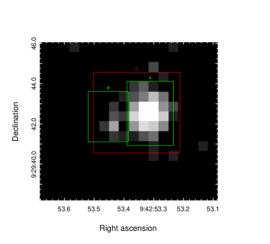
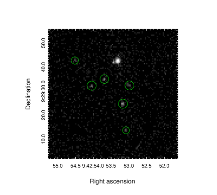
Figure 1.— Left Panel: SN 2010jl field of view (FoV) from Chandra observations. The left green box ($2.0^{\prime\prime}\times 2.5^{\prime\prime}$) marked ‘B’ is used to extract the spectrum for UGC 5189A. The right green box ($2.3^{\prime\prime}\times 3.2^{\prime\prime}$) marked ‘A’ has been used to extract the SN 2010jl spectrum. The largest red box ($4.3^{\prime\prime}\times 4.0^{\prime\prime}$) marked ‘C’ includes both SN 2010jl and the UGC 5189A. Right Panel: Field of view from Chandra observations. Here SN 2010jl is the brightest source at the top part of the image center. The green circles are the 6 nearby sources within a $21\arcsec$ radius centered at the SN 2010jl position, excluding UGC 5189A.

We list the absorbed and unabsorbed fluxes and unabsorbed luminosities of UGC 5189A in the 0.2–10 keV range at five Chandra epochs in Table 2. The flux varies at most by a factor of 1.8 in these epochs, so we refit the data assuming constant flux at all the epochs. This also gives a reasonable fit with a best fit C-statistic of 31.4 for 36 degrees of freedom. Here the best fit values are $N_{H}(\rm Host)=(4.07^{+5.71}_{-4.00})\times 10^{21}$ cm^-2 and $\Gamma=1.15^{+0.42}_{-0.39}$. The 0.2–10 keV absorbed (unabsorbed) flux of UGC 5189A is $(2.02\pm 0.14)\times 10^{-14}$ erg cm^-2 s^-1 ($(2.22\pm 0.16)\times 10^{-14}$ erg cm^-2 s^-1), which translates to an unabsorbed luminosity of $(6.13\pm 0.44)\times 10^{39}$ erg s^-1 (Table 2). We also plot the contour levels of the best fit column density and photon index in Figure 2. We note that there is a large uncertainty in the absorption column density.

The spatial resolution of the Swift-XRT , XMM-Newton and NuSTAR observations are not as good as that of Chandra , so we have to take care of contamination from more distant sources while analyzing these data. We looked for the contaminating sources within a $60^{\prime\prime}$ region centered at SN 2010jl. As shown in the Chandra FOV (right panel of Fig. 1), there are 6 sources within $21^{\prime\prime}$ of the SN position, in addition to UGC 5189A. There are no additional sources between $21^{\prime\prime}$ and $60^{\prime\prime}$ radius centered at the SN. We extracted spectra in the 0.2–10 keV range from Chandra data at each epoch for these 6 sources and carried out a joint fit, assuming the flux did not change at various Chandra epochs. Their spectra are best fit with a column density of $N_{H}(\rm Host)=(4.72^{+3.82}_{-3.06})\times 10^{21}$ cm^-2 and a power law index of $\Gamma=2.05^{+0.43}_{-0.37}$ (reduced $\chi^{2}=1.07$). We note that the absorption column density is similar to that obtained for UGC 5189A, re-confirming that the host galaxy UGC 5189 contributes a significant amount of X-ray absorbing column. The 0.2–10 keV absorbed (unabsorbed) flux of these sources combined is $(2.22\pm 0.11)\times 10^{-14}$ erg cm^-2 s^-1 ($(3.30\pm 0.17)\times 10^{-14}$ erg cm^-2 s^-1), which translates to an unabsorbed luminosity of $(9.11\pm 0.47)\times 10^{39}$ erg s^-1. We also attempted to carry out fits where we let normalizations at each epoch vary. The absorbed flux changed at most by a factor of 2, the reduced $\chi^{2}=0.84$ improved significantly. In Table 3 we give the $0.2-10$ keV fluxes of these sources.

3.2. Analysis of SN 2010jl

Chandra et al. (2012a) analyzed Chandra data from 2010 December and 2011 October observations. In both cases, their best fit temperature values always hit the hard upper limit of the models in XSPEC. The power law models were discarded since they gave an unphysically hard spectrum. Chandra et al. (2012a) preferred a thermal model, noting that the plasma giving rise to the X-ray emission is sufficiently hot that Chandra is not sensitive to the high plasma temperature. However, we now have the advantage of having SN 2010jl observations with NuSTAR which has sensitivity in the range 3–80 keV. Because of the above complications, we use NuSTAR data to determine the shock temperature and then use the same temperature for the analysis of the rest of the data.

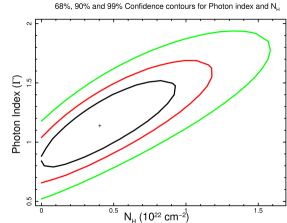
Figure 2.— The 68% (black), 90% (red) and 99% (green) confidence contours for best fit column density ($N_{H}$) and power law photon index ($\Gamma$) for the UGC 5189A X-ray spectra obtained from the joint fit of Chandra data at various epochs (see §3.1). The uncertainty in the column density is large.

3.2.1 NuSTAR data

NuSTAR observed SN 2010jl on 2012 October 5 (Ofek et al., 2014). SN 2010jl was also observed with XMM-Newton on 2012 November 1. To get spectral coverage in a wider energy range, we carried out a joint fit to both NuSTAR and XMM-Newton spectra. We used the best fit parameters of the 2012 June 1 Chandra data for UGC 5189A and the other 6 contaminating sources to subtract out their contamination to SN flux (see §3.1). For the XMM-Newton observations, we used spectra from MOS1, MOS2 and PN CCD arrays, whereas for the NuSTAR observations, we used spectra from both FPMA as well as FPMB focal plane modules. The total absorption column density in the models are $N_{H}$, where $N_{H}=N_{H}(\rm Galactic)+N_{H}(\rm Host)+N_{H}(\rm CSM)$. Here $N_{H}(\rm Galactic)$ and $N_{H}(\rm Host)$ are explained in §3.1 and $N_{H}(\rm CSM)$ is the column density due to the SN CSM. For $N_{H}(\rm CSM)$, we fix the metallicity to be 0.3 solar. The data are best fit with an absorbed thermal plasma model. The reduced $\chi^{2}$ is 0.97 for 165 degrees of freedom. The best fit column density for SN 2010jl is $N_{H}(\rm CSM)=(6.67^{+2.47}_{-1.94})\times 10^{21}$ cm^-2 and the plasma temperature is $kT=18.99^{+8.75}_{-4.86}$ keV. This temperature is consistent with that found by Ofek et al. (2014).

Since Chandra et al. (2012a) claimed the presence of a 6.33 keV Fe $K\alpha$ line in their December 2010 Chandra spectrum, we also attempted to add a Gaussian component around the same energy and refit the spectra. There was no significant change in the quality of the fit. Thus Fe K-$\alpha$ line is not significant here. In Figure 3, we plot the best fit model as well as the contour diagram of $N_{H}(\rm CSM)$ versus $kT$. The 0.2–80 keV absorbed (unabsorbed) flux of the SN is $(5.24\pm 0.25)\times 10^{-13}$ erg cm^-2 s^-1 ($(6.01\pm 0.28)\times 10^{-13}$ erg cm^-2 s^-1). The 0.2–10 keV absorbed (unabsorbed) flux of the SN is listed in Table 5.

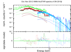
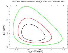
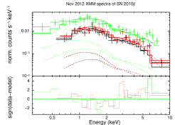
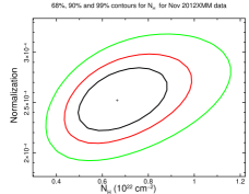
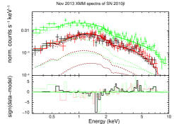
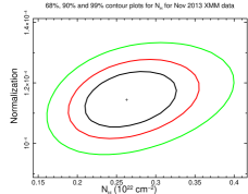
Figure 3.— The spectra of SN 2010jl and their best fit models as described in § 3.2. Upper panel: The best fit model for the 2012 October 6–November 1 joint XMM-Newton (green: PN, black: MOS1, red: MOS2) and NuSTAR (blue: FPMA, cyan: FPMB) spectra. The data are best fit with an absorbed apec model. The right plot shows the 68% (black), 90% (red) and 99% (green) confidence contours for the best fit CSM column density ($N_{H}$) and the plasma temperature ($kT$). Middle panel: The spectrum and column density confidence contours for 2012 Nov 1.63 XMM-Newton data. Lower panel: The spectrum and column density confidence contours for 2013 Nov 1.67 XMM-Newton data. In all the cases, $N_{H}$ is well constrained. The colors in the middle and lower panels have the same association as explained in the top panel. Here the normalized counts s^-1 kev^-1 in the y-axes in the left plots of the spectra are normalized counts s^-1 kev^-1. The word normalized indicates that this plot has been divided by the effective area, the value of the EFFAREA keyword, in the response file associated with each spectrum. In all the left side plots, the residuals are in terms of $\sigma s$ with error bars of size one.

Table 4Best fit models at various epochs

Date of	Instrument	Model	Param-1	Param-2	Param-3	Reduced
Obsn			$N_{H}$ (cm-2)	${N_{H}}_{3}$ (cm-2)		$\chi^{2}$
2010 Nov 5–20	Swift-XRT	$\sum\limits_{i=1}^{2}{N_{H}}_{i}^{*}*\Gamma_{i}+N_{H}^{*}*(kT+\rm Gauss)$	$(17.67^{+16.83}_{-7.91})\times 10^{23}$	$\cdots$	Gauss$=6.39^{+0.19}_{-0.23}$	1.73
2010 Nov 22.03	Chandra	$N_{H}^{*}*kT$	$(9.59^{+2.60}_{-2.16})\times 10^{23}$	$\cdots$	$\cdots$	1.57
2010 Nov 23–Dec 05	Swift-XRT	$\sum\limits_{i=1}^{2}{N_{H}}_{i}^{*}*\Gamma_{i}+N_{H}^{*}*kT$	$9.59\times 10^{23}$ (fixed)	$\cdots$	$\cdots$	1.35
2010 Dec 7–8	Chandra	$N_{H}^{*}*(kT+\rm Gauss)$	$(9.47^{+0.55}_{-0.52})\times 10^{23}$	$\cdots$	Gauss$=6.33^{+0.07}_{-0.05}$	1.90
2011 Apr 24–28	Swift-XRT	$\sum\limits_{i=1}^{2}{N_{H}}_{i}^{*}*\Gamma_{i}+N_{H}^{*}*kT$	$(5.74^{+2.75}_{-2.00})\times 10^{23}$	$\cdots$	$\cdots$	0.92
2011 Oct 17.85	Chandra	$N_{H}^{*}*kT$	$(1.63)\times 10^{23}$	$\cdots$	$\cdots$	2.07
2011 Oct 17.85	Chandra	$N_{H}^{*}*kT+{N_{H}}_{3}^{*}*\Gamma$	$(2.05^{+0.29}_{-0.24})\times 10^{23}$	$4\times 10^{21}$ (fixed)	$\Gamma=1.7$ (fixed)	1.37
2011 Oct 17.85	Chandra	$N_{H}^{*}*kT+{N_{H}}_{3}^{*}*\Gamma$	$(2.89^{+0.26}_{-0.22})\times 10^{23}$	$(3.00^{+1.57}_{-1.20})\times 10^{21}$	$\Gamma=1.7$ (fixed)	1.11
2012 Jun 10.67	Chandra	$N_{H}^{*}*kT$	$(3.74\times 10^{22})$	$\cdots$	$\cdots$	2.71
2012 Jun 10.67	Chandra	$N_{H}^{*}*kT+{N_{H}}_{3}^{*}*\Gamma_{2}$	$(1.11^{+0.22}_{-0.18})\times 10^{23}$	$0.4\times 10^{21}$ (fixed)	$\Gamma_{2}=1.7$(fixed)	0.93
2012 Jun 10.67	Chandra	$N_{H}^{*}*kT+{N_{H}}_{3}^{*}*\Gamma_{2}$	$(1.09^{+0.25}_{-0.20})\times 10^{23}$	$(3.70^{+1.88}_{-1.53})\times 10^{21}$	$\Gamma_{2}=1.7$ (fixed)	0.94
2012 Oct 7–21	Swift-XRT	$\sum\limits_{i=1}^{2}{N_{H}}_{i}^{*}*\Gamma_{i}+N_{H}^{*}*kT$	$6.67^{\times}10^{21}$ (fixed)	$\cdots$	$\cdots$	2.86
2012 Oct 5–Nov 1	NuSTAR ,XMM-Newton	$\sum\limits_{i=1}^{2}{N_{H}}_{i}^{*}*\Gamma_{i}+N_{H}^{*}*kT$	$(6.67^{+2.47}_{-1.94})\times 10^{21}$	$\cdots$	$\cdots$	0.97
2013 Jan 5–Mar 29	Swift-XRT	$\sum\limits_{i=1}^{2}{N_{H}}_{i}^{*}*\Gamma_{i}+N_{H}^{*}*kT$	$(4.03^{+3.32}_{-2.23})\times 10^{21}$	$\cdots$	$\cdots$	1.48
2013 May 14–Jun 28	Swift-XRT	$\sum\limits_{i=1}^{2}{N_{H}}_{i}^{*}*\Gamma_{i}+N_{H}^{*}*kT$	$(5.58^{+5.75}_{-2.78})\times 10^{21}$	$\cdots$	$\cdots$	1.87
2013 Nov 1.67	XMM-Newton	$\sum\limits_{i=1}^{2}{N_{H}}_{i}^{*}*\Gamma_{i}+N_{H}^{*}*kT$	$(2.64^{+0.69}_{-0.59})\times 10^{21}$	$\cdots$	$\cdots$	1.41
2013 Dec 11-30	Swift-XRT	$\sum\limits_{i=1}^{2}{N_{H}}_{i}^{*}*\Gamma_{i}+N_{H}^{*}*kT$	$2.64\times 10^{21}$ (fixed)	$\cdots$	$\cdots$	1.22
2014 Jun 1.25	Chandra	$N_{H}^{*}*kT$	$(6.82^{+3.05}_{-2.25})\times 10^{21}$	$\cdots$	$\cdots$	1.24
2014 May 11-Jun 27	Swift-XRT	$\sum\limits_{i=1}^{2}{N_{H}}_{i}^{*}*\Gamma_{i}+N_{H}^{*}*kT$	$6.82\times 10^{21}$ (fixed)	$\cdots$	$\cdots$	0.65
2014 Nov 30-Dec 24	Swift-XRT	$\sum\limits_{i=1}^{2}{N_{H}}_{i}^{*}*\Gamma_{i}+N_{H}^{*}*kT$	$(1.41^{+12.90}_{-1.40})\times 10^{21}$	$\cdots$	$\cdots$	0.43

Note. — Except for the joint XMM-Newton and NuSTAR spectrum, which gave us the best fit temperature of $kT=18.99^{+8.75}_{-4.86}$ keV, everywhere else the temperature has been kept fixed to a value of 19 keV. The $kT$ corresponding to all the models in the model corresponds to an apec thermal plasma model. The $i=1$ index in ${N_{H}}_{i}$ is for UGC 5189A and $i=2$ for 6 nearby sources within a $21^{\prime\prime}$ error circle centered at the SN position. The parameters with no suffix correspond to the main SN component and parameters with suffix 3 correspond to the extra soft component present in the 2011 October and 2012 June data. We have used ${N_{H}}_{i}^{*}=3\times 10^{20}+{N_{H}}_{i}$, ${N_{H}}^{*}=3\times 10^{20}+{N_{H}}$ and ${N_{H}}_{3}^{*}=3\times 10^{20}+{N_{H}}_{3}$. This is to account for the contribution from Galactic absorption whose metallicity is fixed to solar. For host and CSM contributions, the metallicity is fixed to 0.3 solar. For data with multiple fits, the models in bold are considered to be the models best representing the respective spectra.

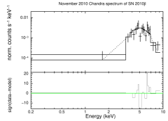
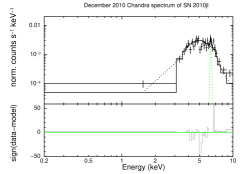
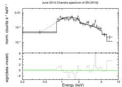
Figure 4.— The best fit models to Chandra spectra of SN 2010jl at 2010 Nov, 2010 Dec and 2014 June, respectively. The best fit models are explained in § 3.2 and listed in Table 4.

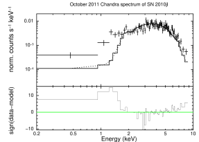
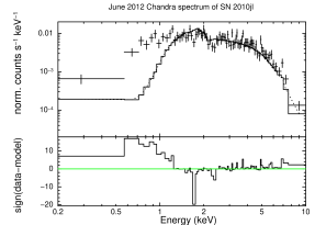
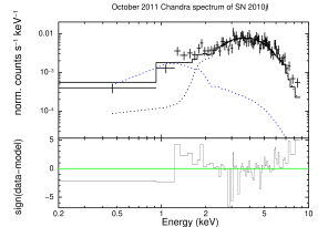
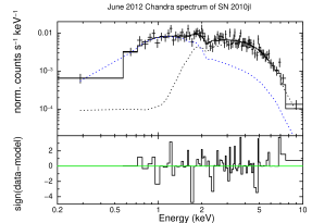
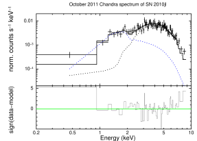
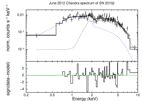
Figure 5.— October 2011 (left panels)and June 2012 (right panels) Chandra spectra of SN 2010jl. These are the two epochs where the evidence of an extra component is present at the lower energy end of the spectra. Left Panels: The Chandra best fit spectra for the 2011 October data. The top row is fit with only a thermal plasma model (black dashed line). The middle row includes an additional absorbed power law model (blue dashed line) and fixing the absorption of the extra component to that of host galaxy’s absorption, i.e. $4\times 10^{21}$ cm^-2. The lower row is the same as the middle row, except the column density has been kept as a free parameter. Right Panels: Same as left, but for SN 2010jl spectra of 2012 June Chandra data.

3.2.2 Chandra data

For all data, we fix the temperature to be $kT=19$ keV (see §3.2.1). Even though this temperature is probably a lower limit to the temperature for the SN shock at earlier epochs, it is the best available temperature estimate. This will probably introduce some errors in the SN flux and the column density estimates. However, we discuss in §5.1 that the uncertainties due to the assumption of constant temperature are not significantly large.

The Chandra data obtained in 2010 November 22 have very few counts, so we group the spectrum into 5 counts per bin and use C-statistics to fit the data. We fix all the parameters except the normalization and $N_{H}$. For a metallicity of 0.3, the data are best fit with a column density of $N_{H}(\rm CSM)=(9.59^{+2.60}_{-2.16})\times 10^{23}$ cm^-2.

The 2010 December 7–8 spectra were grouped in 15 counts per bin and $\chi^{2}$-statistics were applied to obtain best fits. The spectra are best fit with a column density of $N_{H}(\rm CSM)=(9.47^{+0.55}_{-0.52})\times 10^{23}$ cm^-2. However, there is an indication of extra emission component around 6 keV energy, which we also seen by Chandra et al. (2012a) and was associated with Fe K-$\alpha$ line. In our current fits, the line is best fit with a Gaussian of energy $E_{\rm Gauss}=6.33^{+0.07}_{-0.05}$ keV and width 0.19 keV. The 0.2–10 keV unabsorbed flux in this line component is $(4.59\pm 2.53)\times 10^{-14}$ erg cm^-2 s^-1.

The analysis of 2011 October data show that the 6.33 keV iron line is not present in the spectrum, and the CSM column density has now decreased to a value of $N_{H}(\rm CSM)=1.63\times 10^{23}$ cm^-2. A decrease of the column density with time is expected as the shock moves to larger radii. However, the apec model does not fit the SN spectrum well (reduced $\chi^{2}=2.07$ for 73 degrees of freedom, also see Fig. 5). There appears to be an extra component at the lower energy end of the spectrum. We explore three possibilities for this component. First, the component may be coming from the same region as the harder X-ray emission, which is most probably the forward shock. In this case, the column density for the soft extra component, $N_{H}(\rm Soft)$, should be the same as that of the 19 keV component. The second possibility is that this component is arising from the reverse shock. In this case the absorption for this component should be higher than that of the 19 keV component as the cool shell will contribute to an additional absorption. In the third case, we let the $N_{H}$ vary independently. The first and second possibilities seem unlikely because by fixing the column density to either that of the 19 keV component, or declaring the column density associated with the 19 keV component to be the lower limit for this extra component (cool shell origin of the component), neither the apec nor the power law models give a good fit. The best fit models result in an extremely low temperature $<0.1$ keV or negative power law index, and give a 7 orders of magnitude higher normalization than the harder component, which is nonphysical. When we fit the spectra with a power law index of $\Gamma=1.7$ and fix the column density for this extra component to be that of the host galaxy, i.e. $4.1\times 10^{21}$ cm^-2, the reduced $\chi^{2}$ improved from 2.07 to 1.37. Allowing $N_{H}(\rm Soft)$ to vary freely gives a best fit with $N_{H}(\rm Soft)=3.00^{+1.57}_{-1.20}\times 10^{22}$ cm^-2 and the reduced $\chi^{2}$ improves significantly to 1.11. In the case of fixing the column density to the host galaxy absorption, the 0.2–10 keV absorbed (unabsorbed) flux of the extra component is $(3.30\pm 0.67)\times 10^{-14}$ erg cm^-2 s^-1 ($(4.14\pm 1.84)\times 10^{-14}$ erg cm^-2 s^-1). In the case where we let the column density be a free parameter, the 0.2–10 keV absorbed (unabsorbed) flux of the extra component is $(1.22\pm 0.16)\times 10^{-13}$ erg cm^-2 s^-1 ($(2.01\pm 1.27)\times 10^{-13}$ erg cm^-2 s^-1).

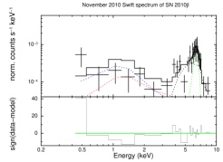
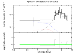
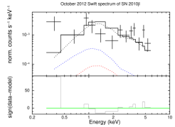
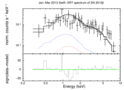
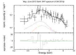
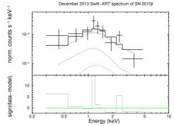
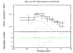
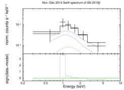
Figure 6.— The best fit Swift-XRT spectra of SN 2010jl at various epochs. The best fit models plotted here are detailed in § 3.2 and listed Table 4. The black dashed line is the best fit apec thermal plasma model. The red line is the contribution of UGC 5189A and the blue line is the contribution from six nearby sources.

Table 5SN 2010jl 0.2–10 keV flux at various epochs

Date of	Telescope	$\Delta t_{exp}$	Abs. Flux	Unabs. Flux	Unabs. Luminosity
Observation		days	erg cm-2 s-1	erg cm-2 s-1	erg s-1
2010 Nov 5–20	Swift-XRT	$43.55\pm 7.53$	$(4.67\pm 0.81)\times 10^{-13}$	$(29.54\pm 7.95)\times 10^{-13}$	$(8.49\pm 2.29)\times 10^{41}$
2010 Nov 22.03	Chandra	53.03	$(7.07\pm 1.15)\times 10^{-13}$	$(30.56\pm 4.95)\times 10^{-13}$	$(8.78\pm 1.42)\times 10^{41}$
2010 Nov 23–Dec 5	Swift-XRT	$60.34\pm 6.33$	$(5.42\pm 1.81)\times 10^{-13}$	$(24.33\pm 8.13)\times 10^{-13}$	$(6.99\pm 2.33)\times 10^{41}$
2010 Dec 7–8	Chandra	$68.61\pm 0.43$	$(7.03\pm 0.52)\times 10^{-13}$	$(29.40\pm 2.48)\times 10^{-13}$	$(8.45\pm 0.71)\times 10^{41}$
2011 Apr 24–28	Swift-XRT	$208.30\pm 1.74$	$(10.70\pm 2.39)\times 10^{-13}$	$(34.68\pm 7.76)\times 10^{-13}$	$(9.96\pm 2.23)\times 10^{41}$
2011 Oct 17.85	Chandra	382.85	$(9.37\pm 0.56)\times 10^{-13}$	$(22.04\pm 1.32)\times 10^{-13}$	$(6.33\pm 0.38)\times 10^{41}$
2012 June 10.67	Chandra	619.67	$(5.70\pm 0.40)\times 10^{-13}$	$(10.13\pm 0.70)\times 10^{-13}$	$(2.91\pm 0.20)\times 10^{41}$
2012 Oct 7–21	Swift-XRT	$745.17\pm 7.15$	$(3.48\pm 0.81)\times 10^{-13}$	$(4.26\pm 1.00)\times 10^{-13}$	$(1.22\pm 0.29)\times 10^{41}$
2012 Oct 5–Nov 1	NuSTAR , XMM	$750.31\pm 13.33$	$(3.64\pm 0.17)\times 10^{-13}$	$(4.00\pm 0.18)\times 10^{-13}$	$(1.15\pm 0.06)\times 10^{41}$
2013 Jan 21–Mar 29	Swift-XRT	$877.69\pm 33.59$	$(3.40\pm 0.43)\times 10^{-13}$	$(4.00\pm 0.51)\times 10^{-13}$	$(1.15\pm 0.12)\times 10^{41}$
2013 May 14–Jun 28	Swift-XRT	$980.01\pm 22.33$	$(2.73\pm 0.39)\times 10^{-13}$	$(3.29\pm 0.48)\times 10^{-13}$	$(0.95\pm 0.14)\times 10^{41}$
2013 Nov 1.67	XMM-Newton	1128.67	$(1.88\pm 0.07)\times 10^{-13}$	$(2.15\pm 0.08)\times 10^{-13}$	$(0.62\pm 0.02)\times 10^{41}$
2013 Dec 11–30	Swift-XRT	$1178.11\pm 9.57$	$(1.50\pm 0.49)\times 10^{-13}$	$(1.72\pm 0.56)\times 10^{-13}$	$(0.49\pm 0.16)\times 10^{41}$
2014 Jun 1.25	Chandra	1340.25	$(1.53\pm 0.13)\times 10^{-13}$	$(1.82\pm 0.15)\times 10^{-13}$	$(0.52\pm 0.04)\times 10^{41}$
2014 May 11–Jun 27	Swift-XRT	$1343.01\pm 23.89$	$(1.22\pm 0.47)\times 10^{-13}$	$(1.49\pm 0.58)\times 10^{-13}$	$(0.43\pm 0.17)\times 10^{41}$
2014 Nov 30–Dec 24	Swift-XRT	$1535.60\pm 12.90$	$(0.64\pm 0.04)\times 10^{-13}$	$(0.72\pm 0.44)\times 10^{-13}$	$(0.21\pm 0.13)\times 10^{41}$

Note. — Here the fluxes and luminosities are in the 0.2–10 keV range. The fluxes are derived as detailed in §3.2. The SN explosion date is assumed to be 2010 October 1.

Now we carry out an analysis of the 2012 June Chandra spectrum. Here the column density is best fit with a value of $N_{H}(\rm CSM)=3.74\times 10^{22}$ cm^-2. The low temperature feature seen in the 2011 October data is prominent here as well and the reduced $\chi^{2}$ for the absorbed thermal plasma is quite large ($\chi^{2}=2.71$ for 80 degrees of freedom). For this additional low temperature component, we explore the same three possibilities as discussed in the above paragraph for the case of 2011 October data. In the first case, when $N_{H}(\rm Soft)$ is fixed to a value the same as that for the 19 keV component, i.e. $N_{H}(\rm CSM)=3.74\times 10^{22}$ cm^-2, the best temperature goes to very low values $kT\ll 0.1$ keV. In the case of powerlaw fits, the power law index becomes negative, and the normalization becomes unphysically high. When we fit the spectra by fixing the column density for the extra component to be the same as that of host galaxy, the reduced $\chi^{2}$ improved significantly, from 2.71 to 0.94. However, if we let $N_{H}(\rm Soft)$ vary freely, it did not change significantly from that of host galaxy column density value, and the reduced $\chi^{2}$ did not improve. When we kept the column density fixed to the host galaxy value, the 0.2–10 keV absorbed (unabsorbed) flux of the extra component was $(1.58\pm 0.67)\times 10^{-13}$ erg cm^-2 s^-1 ($(1.99\pm 0.17)\times 10^{-13}$ erg cm^-2 s^-1). If we let the column density vary, the 0.2–10 keV absorbed (unabsorbed) flux of the component is $(1.55\pm 0.14)\times 10^{-13}$ erg cm^-2 s^-1 ($(1.93\pm 0.17)\times 10^{-13}$ erg cm^-2 s^-1).

If we assume that the column density of the extra component is fixed to $N_{H}(\rm Host)$ in both the 2011 October and 2012 June data, then the component is much stronger at the later epoch. Surprisingly this component is not present in the 2014 June Chandra data. If we let the column density be a free parameter, then the flux is roughly constant. We do not understand a process that can increase the flux by almost a factor 5 between 2011 October and 2012 June and then vanish completely. Thus we consider the varying column density model to be the more realistic model for this extra component. As per our fits, the component appeared around 2011 October, then became optically thin (reduced absorption consistent with the host galaxy absorption), and finally disappeared. The fits to 2011 October and 2012 June data are plotted in Fig. 5.

In the 2014 June Chandra data the SN component is fitted with the absorbed apec model and the best fit column density is $N_{H}(\rm CSM)=(6.82^{+3.05}_{-2.25})\times 10^{21}$ cm^-2. Initially we let the temperature be a free parameter, to check if the forward shock cooled down significantly or if the reverse shock too has started to contribute towards X-ray emission. But the best fit temperature again hit the model upper limit of 80 keV, so we fixed it to $kT=19$ keV as in previous datasets. The best fit absorbed apec model gives a reduced $\chi^{2}=1.15$. The extra component seen in the 2011 October and 2012 June data is no longer detectable. The best fit models are listed in Table 4, and the best fits for all the Chandra data except for those from 2011 October and 2012 June are shown in Fig. 4. The best fit models for the 2011 October and 2012 June data are plotted in Fig 5.

3.2.3 XMM-Newton data

For the XMM-Newton observations, we use the best fit models of UGC 5189A and the contaminating sources from the 2014 June Chandra data (nearest in time to XMM-Newton observations) to remove the contamination in SN flux estimation. We again use an absorbed thermal plasma model to fit the SN spectra as described in §3.2.2. The data are best fit with $N_{H}(\rm CSM)=(2.64^{+0.69}_{-0.59})\times 10^{21}$ cm^-2 with a reduced $\chi^{2}=1.41$. We plot the spectrum and contour plots in the lower panel of Fig. 3.

3.2.4 Swift-XRT data

The Swift-XRT observations are usually closely spaced in time but with short ($<10$ ks) exposure times. To increase the detection significance, we combine several data sets to extract the spectra near-simultaneously. Our criterion to group the spectra was to get a uniform coverage on a logarithmic scale. We, therefore, group the observations taken during 2010 November 5-20, 2010 November 23-December, 2011 April, 2012 October, 2013 January-March, 2013 May-June, 2013 December, 2014 May-June, and 2014 November-December. The spectra were extracted using the online Swift-XRT spectrum extraction tool (Evans et al., 2009; Goad et al., 2007). We fitted the apec model with a fixed temperature of 19 keV and C-statistics were used. In 2012 October data (10.7 ks), 2013 December data (14.6 ks), and 2014 May–June data (13.1 ks), there are only 67, 46 and 35 counts, respectively, so we fixed $N_{H}(\rm CSM)$ to that of the best fit values closest in time, obtained from analysis of data of other telescopes. The Swift-XRT spectra are plotted in Fig. 6.

In the 2010 November Swift-XRT data (Fig. 6), there is a clear indication of an extra feature around 6 keV, which was also seen in the Chandra data around the same epoch. A Gaussian is best fit with an energy of $E_{\rm Gauss}=6.39^{+0.19}_{-0.23}$ keV. The unabsorbed 0.2-10 keV fluxes in the Gaussian and the continuum components are $(3.39\pm 1.28)\times 10^{-13}$ erg cm^-2 s^-1 and $(26.15\pm 6.67)\times 10^{-13}$ erg cm^-2 s^-1, respectively. In 2010 Dec data we attempted to add a Gaussian, since it was also seen in the 2010 December Chandra data. However, the data have very few counts thus the fits statistics do not change significantly.

The best fit SN 2010jl models from our analysis are listed in Table 4. The 0.2–10 keV flux values are given in Table 5. In Fig. 7, we plot the evolution of the 0.2–10 keV luminosity as well as the column density. For the first 300 days, both quantities evolve slowly, but after 300 days, one can see a steep power law decline (decay index $\sim 2$) in the luminosity.

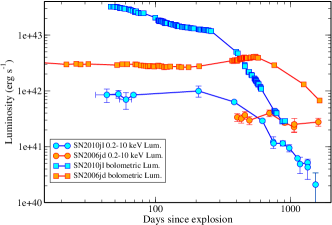
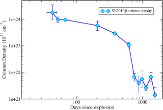
Figure 7.— In the top panel, we plot the 0.2–10 keV light curve for SN 2010jl (Blue filled circles). We plot the bolometric light curve taken from Fransson et al. (2014) in blue squares. We also plot the X-ray light curve (Chandra et al., 2012b) and bolometric luminosity (Stritzinger et al., 2012) of another well studied Type IIn supernova, SN 2006jd (orange circles and squares, respectively). Unlike SN 2010jl which has a very steep X-ray decay with index of $-2.12$, the SN 2006jd decline is very flat (index $-0.26$) in a similar time range. In the lower panel we plot the evolution of the CSM column density for SN 2010jl as explained in Section 3.2.

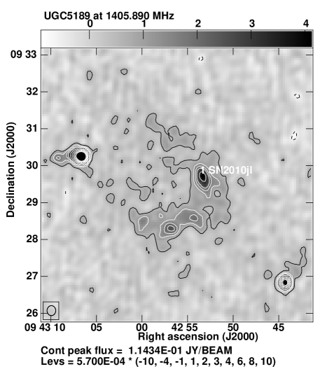
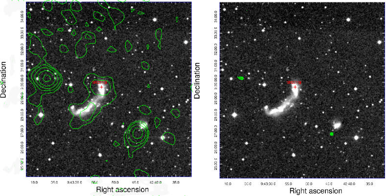
Figure 8.— Upper Panel: Pre-explosion SN 2010jl FoV image with the VLA in the 1400 MHz band. The flux units in the upper color bar are mJy. SN 2010jl is at a position $\alpha=09^{h}42^{m}53^{s}.337$, $\delta=+09^{o}29^{\prime}42.^{\prime\prime}13$ (J2000). The immediate SN 2010jl region and UGC 5189A are indistinguishable as the image resolution is $16^{\prime\prime}\times 14^{\prime\prime}$. Lower panel: The overlay NVSS ($45^{\prime\prime}$ resolution; left side) and FIRST ($5^{\prime\prime}$ resolution; right side) images on the J-band POSS II (Palomer Transient Survey II) image with the same contour levels. Much of the extended emission is absent in the higher resolution image.

4. RADIO ANALYSIS

Before analyzing the SN 2010jl data, we examine the radio emission in the SN FoV in Very Large Array (VLA) archival data taken during 2006 December 1–21 in 1.4 GHz band. The telescope at the time of these observations was in C-configuration. The duration for all the datasets ranged from 30 minutes to 3 hours (including the calibrator). We carried out a joint analysis of the data. The image resolution obtained was $16^{\prime\prime}\times 14^{\prime\prime}$ and the map rms was 191 $\mu$Jy (Fig. 8). The figure shows that SN 2010jl lies in a region of extended radio emission. To investigate the nature of the radio emission, we looked into the VLA NVSS (resolution $45^{\prime\prime}$) and FIRST (resolution $5^{\prime\prime}$) images of the SN FoV in the 1.4 GHz band. In Fig. 8, we overlay the Second Palomar Observatory Sky Survey (POSS II) J-band gray image with the NVSS and the FIRST contours. The figure suggests that the extended emission is resolved at higher resolutions and not likely to contaminate the SN flux.

The first radio data of SN 2010jl were taken on 2010 November 6.59 UT in EVLA C-configuration at 8 GHz band. The total duration of the observation including overheads was 30 minutes. The data quality was good and only 7.5% of the data were flagged. The map rms in the 8 GHz band was 24 $\mu$Jy and the synthesized beam size was $2.35^{\prime\prime}\times 2.07^{\prime\prime}$. We did not detect SN 2010jl. The flux density at the SN 2010jl position was $-41\pm 24$ $\mu$Jy. We then attempted to observe the SN 2010jl in 33 GHz band to account for the scenario in which the SN was absorbed at lower frequencies. The observations were taken on 2010 November 8.47 UT for 3588.7 s. We obtained a rms of 45 $\mu$Jy and image resolution of $0.67^{\prime\prime}\times 0.60^{\prime\prime}$. We did not detect SN 2010jl in this band either. The flux density at 33.56 GHz at the SN 2010jl position was $52\pm 45$ $\mu$Jy.

We continued to observe SN 2010jl at regular intervals. The first detection of the SN came on 2012 April 18 in the 22 GHz band, with a flux density of $60.9\pm 17.6$ $\mu$Jy. To estimate the flux density of SN 2010jl in all the images, we fit two Gaussian models, one for the SN component and one for the underlying background level to take care of any underlying extended emission. Since then we have been detecting SN 2010jl in various VLA bands (Table 6). Our most secure detections are in 2012 December, when the VLA was in the A-configuration.

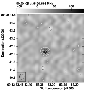
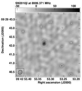
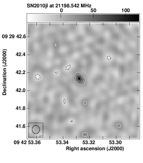
Figure 9.— VLA A-configuration 5 GHz, 8 GHz and 21 GHz detections of SN 2010jl, taken on 2012 Dec 01.46, 02.40 and 02.53, respectively. The units of the color bars above the maps are $\mu Jy$.

Table 6VLA radio observations of SN 2010jl

Date of	Days since	Config.	Central	BW	Resolution	Flux density	rms
obsn. (UT)	Explosion		GHz	Freq, GHz	(${}^{\prime\prime}\times^{\prime\prime}$)	$\mu$Jy	$\mu$Jy
2010 Nov 06.60	37.60	C	8.46	0.26	$2.35\times 2.07$	$<71.1$	23.7
2010 Nov 08.48	39.48	C	33.56	0.26	$0.67\times 0.60$	$<133.5$	44.5
2010 Nov 08.52	39.52	C	22.46	0.26	$0.93\times 0.85$	$<74.4$	24.8
2010 Nov 14.52	45.52	C	22.46	0.26	$0.93\times 0.86$	$<82.8$	27.6
2010 Nov 23.43	54.43	C	22.46	0.26	$1.06\times 0.92$	$<70.1$	23.4
2011 Jan 21.26	113.26	CnB	7.92	0.13	$3.71\times 0.84$	$<76.8$	25.6
2011 Jan 21.26	113.26	CnB	4.50	0.13	$6.52\times 1.51$	$<116.7$	38.9
2011 Jan 21.39	113.39	CnB	22.40	0.26	$0.98\times 0.78$	$<107.4$	35.8
2011 Jan 22.26	114.26	CnB	22.46	0.26	$1.03\times 0.37$	$<79.8$	26.6
2011 Jan 23.27	115.27	CnB	4.50	0.13	$5.26\times 1.63$	$<76.2$	25.4
2011 Jan 23.27	115.27	CnB	7.92	0.13	$2.93\times 0.91$	$<55.5$	18.5
2011 Apr 22.25	204.25	B	22.46	0.26	$0.41\times 0.28$	$<114.0$	38.0
2011 Jul 07.99	280.99	A	4.50	0.13	$0.60\times 0.42$	$<78.0$	26
2011 Jul 07.99	280.99	A	7.92	0.13	$0.27\times 0.22$	$<62.1$	20.7
2012 Jan 24.28	481.28	DnC$\rightarrow$C	8.46	0.26	$3.35\times 2.46$	$<123$	23.4
2012 Feb 28.20	516.20	C	8.55	1.15	$2.65\times 2.16$	$<32.1$	10.7
2012 Mar 02.22	519.22	C	5.24	1.54	$3.89\times 3.53$	$<33.6$	11.2
2012 Apr 15.03	563.03	C	8.68	1.41	$2.77\times 2.25$	$<45.6$	15.2
2012 Apr 15.05	563.05	C	5.50	2.05	$3.89\times 3.29$	$<32.7$	10.9
2012 Apr 18.03	566.03	C	21.20	2.05	$1.13\times 0.98$	$60.9\pm 17.6$	10.1
2012 Apr 22.10	570.10	C	21.20	2.05	$1.08\times 0.87$	$38.3\pm 20.7$	13.5
2012 Aug 11.71	681.71	B	9.00	2.05	$0.84\times 0.71$	$76.6\pm 20.3$	12.9
2012 Aug 12.71	682.71	B	5.50	2.05	$1.26\times 1.08$	$111.9\pm 17.8$	12.6
2012 Dec 01.46	793.46	A	5.50	2.05	$0.34\times 0.30$	$131.3\pm 22.1$	11.1
2012 Dec 02.40	794.40	A	9.00	2.05	$0.24\times 0.22$	$118.8\pm 16.8$	9.8
2012 Dec 02.53	794.53	A	21.20	2.05	$0.09\times 0.08$	$115.3\pm 17.1$	9.9
2013 Jan 18.34	841.34	A$\rightarrow$D	21.20	2.05	$0.17\times 0.05$	$<109$	10.7
2013 Jan 18.38	841.38	A$\rightarrow$D	9.00	2.05	$0.32\times 0.12$	$<470$	20.9
2013 Jun 10.96	984.96	C	8.68	2.05	$2.31\times 2.03$	$123.0\pm 26.8$	9.7
2013 Jun 11.94	985.94	C	5.50	2.05	$3.98\times 3.23$	$91.3\pm 34.8$	12.7
2013 Aug 10.74	1045.74	C	21.20	2.05	$1.09\times 0.90$	$<69.3$	23.1

To determine the SN 2010jl position, we have used 2012 December 2 data in 22 GHz band when the VLA was in A-configuration. In this data, we obtained a resolution of $0.09^{\prime\prime}\times 0.08^{\prime\prime}$. The best SN position is $\alpha=09^{h}42^{m}53.^{s}32773\pm 0.00021$, $\delta=+09^{o}29^{\prime}42.^{\prime\prime}13330\pm 0.00344$ (J2000), which agrees well within 0.15^′′ accuracy with the optical position given by Ofek et al. (2014).

The post detection observations of SN 2010jl with the VLA C-configuration in 2013 June were contaminated by the extended flux due to poorer resolution in this configuration, especially in the 5 and 8 GHz bands. In this case, we have used the C-configuration images of 2012 February before the SN 2010jl detection in the respective frequencies and subtracted it from the post detection images to get the uncontaminated flux of SN 2010jl.

In Fig. 9, we plot the contour plots of SN 2010jl in the 5 GHz, 8 GHz and 21 GHz bands for this epoch. The SN flux densities obtained in 2013 Jan when the VLA was in A$\rightarrow$D configuration are not very reliable due to contamination from the underlying extended emission.

In Fig. 10, we plot the light curves of the SN (upper panel), and in the lower panel plot the spectra at 3 epochs when the SN was detected in multiple bands. For the spectra with the JVLA data, we have divided the 2 GHz bandwidth into 2 subbands and imaged it independently to get the flux densities in the two subbands.

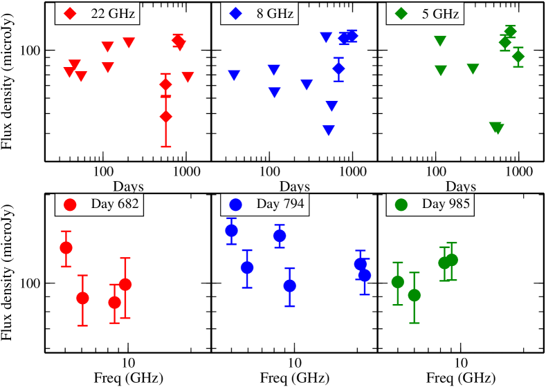
Figure 10.— Radio light curves of SN 2010jl are shown in the upper panel. The inverted triangles are $3\sigma$ upper limits. The lower panel shows the radio spectrum at 3 epochs.

5. DISCUSSION

Using the NuSTAR data, we derive a shock temperature of 19 keV, which is consistent with the analysis of Ofek et al. (2014). This corresponds to a shock velocity of $\sim 4000$ $\rm~{}km\,s^{-1}$ at around 750 days. At earlier epochs, the shocked gas may be hotter, but we cannot determine the exact temperature at any other epoch due to the absence of hard X-ray observations. This may introduce some errors in column density estimate and the SN flux. We attempt to quantify this error. In a standard SN-CSM interaction model, the temperature of the shock varies with time $t$ as $t^{-2/(n-2)}$ (where $n$ is the power-law index of the ejecta density profile), i.e. $t^{-0.25}$ for a typical value $n=10$ (Chevalier & Fransson, 2003). Thus over the full span of our observations (day $\sim$50 to $\sim$1500), the temperature would change by a factor of $\sim 2$. In our fits, we estimate the change in column density and in SN flux due to the change in temperature. We find that for a 20% change in temperature, the column density changes by 5 % and the SN flux changes by $1.5$ %. If we change the temperature of the shock by 100 %, the change in column density is less than 15 % and in the SN flux is less than 10 %. This analysis shows that even though we do not have a handle on the temperature at various epochs and are assuming a constant temperature, the errors introduced in other parameters like column density and the SN flux do not suffer significantly.

5.1. Summary of main results

SN 2010jl is the only Type IIn SN for which a well sampled X-ray dataset exists. Thus we are able to trace the evolution of column density and light curve all the way from 40 to 1500 days (Fig. 7).

The X-ray luminosity for SN 2010jl is roughly constant for the first $\sim 200$ days with a power law index of $0.13\pm 0.08$. Unfortunately there are no data between 200 to 400 days, but from day 400 onwards one can see a faster decay in the luminosity following a powerlaw index of $-2.12\pm 0.13$. For a shock velocity of 4000 km s^-1 estimated above, the start of the rapid decline in X-rays corresponds to a radius of $1.3\times 10^{16}$ cm. In Fig. 7, we overplot the bolometric luminosity lightcurve of SN 2010jl taken from Fransson et al. (2014) on the X-ray light curve of the SN. We note that the bolometric luminosity also declines rapidly around day 300, consistent with the X-ray lightcurve. Fransson et al. (2014) have argued that the steepening in the bolometric luminosity coincides with the H$\alpha$ shift becoming constant and have explained it a result of less efficient radiative acceleration. Ofek et al. (2014) argue that this is the time when the SN reached the momentum conserving snow-plow phase. However, as we will show in Section 5.2, this can be explained in our simple model by changes in the CSM density profile.

In Fig. 7, we also plot the X-ray and bolometric luminosities of another well sampled Type IIn, SN 2006jd (Chandra et al., 2012b; Stritzinger et al., 2012). The luminosity decline is much flatter in SN 2006jd than that of SN 2010jl. Around the same epoch, the SN 2006jd X-ray lightcurve declines as $t^{-0.24}$, while SN 2010jl declines as $t^{-2.12}$. The relative flatness of the bolometric luminosity of SN 2006jd for a longer duration indicates that the CSM interaction powered the light curve for a much longer time than SN 2010jl . This indicates that the duration of mass ejection in SN 2006jd may have been longer in this case than for SN 2010jl, though in both cases occurred shortly before the explosion. This suggests different nature of progenitors for the two SNe.

The most interesting result of the paper is the evolution of the column density with time. At $t\sim 40$ days, the column density is 3000 times higher than the Galactic column density, and declines by a factor of $\sim 100$ by the epoch of our last observation in 2014 Dec. Since the higher column density is not associated with the high host galaxy extinction, this indicates that the higher column density is due to the CSM in front of the the shock where the dust is evaporated, thus is arising from the CSM.

The presence of broad emission lines seen in early SN 2010jl optical spectra (Smith et al., 2012; Fransson et al., 2014; Ofek et al., 2014) can be explained by electron scattering (Chugai, 2001). This requires an electron scattering optical depth $>1-3$, i.e. a column density greater than $3\times 10^{24}$ cm^-2. Comparable values of the column density were seen only in the first X-ray observations ($t<70$ d; Table 4). At later epochs ($t>70$ d) we only see the X-rays which pass through a column density $<10^{24}$ cm^-2. These constraints are difficult to reconcile with a spherical model of the column density $\sim 3\times 10^{24}$ cm^-2. We therefore should admit that either the width of emission lines at the late time is not related to Thomson scattering, or the X-rays escape the interaction region avoiding the CSM with a high column density. Thus, a possible scenario for the CSM in SN 2010jl is the same as the bipolar geometry in the CSM of $\eta$–Carinae (Smith, 2006).

An intriguing issue here is the presence of an extra component in the 2011 October and 2012 June Chandra data, which is not present before or after. This component is well fit with a power law index of 1.7, though with a varying column density, with much higher column density at the 2011 October epoch. The origin of this component is not clear. However, the component seems to spatially coincide with the the position of the SN and occurs when there are changes to the SN spectrum in the energy range close to that of the extra component. This would seem to suggest that the emission is related to the SN. One possibility is that the soft component is a result of a cooling shock. In this scenario a mass loss rate of $0.1M_{\odot}$yr^-1 (Fransson et al., 2014), wind velocity $\sim 100$ $\rm~{}km\,s^{-1}$ (Fransson et al., 2014), and shock temperature of 19 keV (this paper) corresponds to a cooling time of 86 days at $10^{16}$ cm (roughly the radius at one yr for ejecta velocity of 4000 $\rm~{}km\,s^{-1}$). Thus the forward shock should be cooling around this time, as mentioned in our discussion of the optical light curve. An adiabatic shock model underestimates the low energy X-ray flux. The fact that the need for an additional component disappears could be a result of the shock becoming adiabatic.

While the radio observations of SN 2010jl started as early as $\sim 40$ days post explosion, the first radio detection was around day 566. Unlike its X-ray counterpart, the radio luminosity from SN 2010jl is weak for a SN IIn (Fig. 10). This is unlike SN 2006jd which was an order of magnitude brighter in radio bands than SN 2010jl (Chandra et al., 2012b). Like most of the known radio Type IIn SNe, SN 2010jl rises at radio wavelengths at late times, most likely due to absorption by a high density of CSM, or due to internal absorption (e.g., Chandra et al., 2012b). We have not attempted to fit a detailed model to the radio data in view of the small number of detections and small range of time. However, the existing data have distinctive features as seen in Fig.  10. The light curves are fairly flat, as are the frequency spectra. For the standard models of radio SNe, these properties occur when the SN is making the transition from optically thick to optically thin (e.g., Weiler et al., 2002; Chevalier & Fransson, 2003). Thus, most likely we have detected the radio emission near the peak of the synchrotron emission.

From Fig. 10, we estimate that the light curve peak at 5 GHz occurs on about day 900 at a flux of $F_{ob}\approx 0.12$ mJy, or a luminosity of $3.4\times 10^{27}$ ergs s^-1 Hz^-1. The time of maximum is typical of SNe IIn, but the luminosity is lower than most, suggesting that the absorption mechanism is not synchrotron self absorption if the radio emitting region is expanding at $4000-6000\rm~{}km\,s^{-1}$ as indicated by X-ray (this paper and Chandra et al., 2012a) and near IR observations (Borish et al., 2015). This can be seen in Fig. 1 of Chevalier (2009). In the case of the Type IIn SN 1986J, the radio expansion was measured by VLBI techniques and an expansion velocity of $5700\pm 1000\rm~{}km\,s^{-1}$ was found over the period 1999-2008 (Bietenholz et al., 2010). Thus an expansion velocity of $5000-6000\rm~{}km\,s^{-1}$ is plausible. In this case, the absorption would have to be something other than synchrotron self-absorption, most likely free-free absorption. The fact that the 8 GHz radio flux appears around day 700 implies the emission measure along the line of sight at this stage $\langle n_{e}^{2}\ell\rangle\sim 8\times 10^{26}$ cm^-5, where $\ell$ is the linear size of the absorbing gas region and assuming $T_{e}=10^{4}$ K. On day 700 the radius of the shell with an average velocity of 4000 km s^-1 is of $r\sim 2.4\times 10^{16}$ cm. Adopting $\ell\sim r$ we thus come to the rough estimate of the column density $N_{H}\approx 4\times 10^{21}x^{-1}$ cm^-2, where $x$ is the hydrogen ionization fraction. A low hydrogen ionization fraction of $x\sim 0.1$ is needed for the value of $N_{H}$ to be consistent with the column density on day 700 recovered from the X-ray data ($3\times 10^{22}$ cm^-2). Although we expect the CSM to be ionized at early times, recombination is possible at later times; however, a detailed study of the ionization balance in the CSM of SN 2010jl is beyond the scope of this paper.

Another possibility for explaining the escape of the radio emission is that it comes from a different region than the X-ray emitting region. To have a lower column, the radio region would probably come from expansion into a lower density part of the CSM and would thus be more extended. The X-ray emission from the radio region may not be detected because of the low density. Again, details are beyond the scope of this paper.

5.2. Circumstellar interaction modeling

The detailed evolution of the absorbing column density derived from the X-ray data provides us with an unprecedented opportunity to examine the CSM around a SN IIn in both X-ray and optical bands. The question arises of whether the optical light curve powered by the CSM interaction is consistent with the observed column density. Here, we present a simple circumstellar interaction model which suggests that freely expanding SN ejecta collide with the dense CSM. In a smooth dense CSM the interaction zone consists of a forward and a reverse shock along with a cool dense shell (CDS) formed in-between. We confine ourselves to the interaction hydrodynamics based on the thin shell approximation (Chevalier, 1982). The equations of motion and mass conservation are integrated for arbitrary density distributions in both ejecta and CSM using a 4th order Runge-Kutta scheme. The model provides us with the CDS radius ($R_{s}$) and velocity ($v_{s}$), the forward shock speed $v_{fs}\approx v_{s}$, the reverse shock speed $v_{rs}=(R/t-v_{s})$, and the kinetic luminosity released in the shock $L_{j}=2\pi R_{s}^{2}\rho_{j}v_{j}^{3}$, where $\rho_{j}$ is preshock density and $v_{j}$ is the shock velocity ($j=rs,fs$).

Generally, the conversion of the kinetic energy into the radiation in the interaction SNe is affected by complicated hydrodynamic and thermal processes including the thin shell instability (Vishniac, 1994), the Rayleigh-Taylor instability of the decelerating CDS, the CSM clumpiness, mixing, and energy exchange between cold and hot components via radiation and thermal conductivity. This makes the computation of the radiation output of the CS interaction quite a formidable task. We use a simple approach in which the X-ray luminosity of both shocks is equal to the total kinetic luminosity times the radiation efficiency $\eta=t/(t+t_{c})$, where $t_{c}$ is the cooling time of the shocked CSM at the age $t$. To calculate the shock cooling time we assume a constant postshock density four times the upstream density $\rho_{0}$, while the shock temperature is calculated in the strong shock limit. We find that the reverse shock is always fully radiative in our models. In the case of SN 2010jl, the optical luminosity dominates the observed X-ray luminosity by a factor of ten. In our model, the bolometric luminosity, which is primarily in the optical, is equal to the total radiation luminosity.

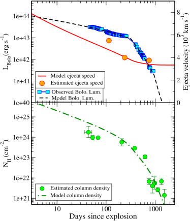
Figure 11.— Top Panel: The bolometric light curve obtained from our modeling detailed in §5.2 (dashed line) plotted over the observational data (blue squares) which are taken from Fransson et al. (2014). The red solid line is the shell velocity obtained from our modeling (in units of $10^{3}$ km s^-1) compared to the observational data (filled circles) taken at various epochs (this paper on day 750 and Borish et al., 2015, at earlier epochs). Lower Panel: the CSM column density outside the forward shock obtained from our modeling in §5.2 versus the data recovered from X-ray observations (squares). Our simple model detailed in §5.2 is able to reproduce the observational quantities quite well.

The model assumes that the optical radiation generated in the interaction zone instantly escapes the CSM which means that the diffusion time ($t_{dif}\sim(r/c)\tau$, where $c$ is the speed of light and and $r$ is the shell radius, Chevalier, 1981) is smaller than the expansion time, or the CSM optical depth $\tau<c/v$ (where $v$ is the shell speed). In our model, on day 3 the column density of the wind is $5\times 10^{25}$ cm^-2 and the Thomson optical depth at this stage is therefore 30. This value is comparable to $c/v\sim 30$ assuming $v=10^{4}$ $\rm~{}km\,s^{-1}$. Therefore, after about day 3 the diffusive trapping of photons in the wind can be ignored. The SN ejecta density distribution is approximated by the analytical expression $\rho_{e}\propto 1/[1+(v/v_{0})^{n}]$ which reflects an inner plateau ($v<v_{0}$) and an outer power law density drop with $7\leq n<10$. The initial ejecta boundary velocity $v_{b}$ is assumed to be $3\times 10^{4}$ km s^-1; our results are not sensitive to the boundary velocity in the range of $(1-3)\times 10^{4}$ km s^-1 at epochs $t>5$ d. The CSM density distribution is set by a broken power law $\rho\propto r^{-m}$ with $m=m_{1}=2$ in the range of $r<r_{1}$ and $m=m_{2}>2$ for $r>r_{1}$. The value $m_{1}=2$ was chosen for small radii because it is an approximate fit and is plausible for a wind; the outer value of $m_{2}$ is a fitting parameter. The ejecta diagnostics based on the CSM interaction cannot constrain the ejecta mass and energy uniquely because the same density versus velocity distribution in the ejecta outer layers can be produced by a different combination of mass and energy. Yet the observed interaction luminosity and the final velocity of the decelerated shell ($v_{f}$) constrain the energy of the outer ejecta with the velocity $v>v_{f}$. For the adopted density power law index $n$ the obvious relations $v_{0}\propto(E/M)^{1/2}$, $\rho(v)\propto\rho_{0}(v_{0}/v)^{n}$, and $\rho_{0}\propto M/v^{3}$ result in the energy-mass scaling $E\propto M^{(n-5)/(n-3)}$, or $E\propto M^{0.6}$, assuming $n=8$. In turn, this scaling, when combined with the requirement that the velocity $v_{f}$ should be larger than the ejecta density turnover velocity $v_{0}$, provides us with the lowest plausible values of $E$ and $M$. As a standard model we adopt an ejecta mass of $8~{}M_{\odot}$ which barely satisfies the condition $v_{f}>v_{0}$. The corresponding kinetic energy of ejecta is then $2.1\times 10^{51}$ erg.

The optimal model is found by the $\chi^{2}$-minimization in the parameter space of $r_{1}$, $m_{2}$, and the wind density parameter $w_{1}=4\pi r^{2}\rho$ in the region $r<r_{1}$. We found the best-fitting values $w_{1}=4.1\times 10^{17}$ g cm^-1, $r_{1}=1.29\times 10^{16}$ cm, and $m_{2}=4.45$. The parameter errors determined via $\chi^{2}$ variation do not exceed 1.5 %. These errors are formal and too optimistic, since we ignore uncertainties in the distance and the extinction, and the systematic error related to the model assumptions. The model (Fig. 11) reproduces the SN 2010jl bolometric light curve (obtained from Fransson et al., 2014) quite well and produces reasonble values for the shell velocity, consistent with the observational estimates (obtained from this paper on day 750 and Borish et al., 2015, for the earlier two epochs). The evolution of the column density obtained from X-ray data is also described by our model at $t\geq 200$ d as well, except for the early epoch $t<100$ d when the model requires a somewhat larger column density. In the model, the CSM density power law index breaks at $r_{1}=1.3\times 10^{16}$ cm from $m=2$ to $m=4.45$, which suggests that the bulk, $2.6~{}M_{\odot}$, of the total CSM mass, $3.9~{}M_{\odot}$, lies within the radius $r_{1}$. In order to describe the column density at late epoch $t>600$ d, the power law index should become steeper ($m\approx 7.5$) for $r>r_{2}=3.2\times 10^{16}$ cm. A lower density region outside the close-in CSM is consistent with what is deduced by Fransson et al. (2014) in their analysis for the narrow lines.

The agreement between the optical model CSM column density and that inferred from X-ray data suggests that the CSM density recovered in the model is realistic. The external radius of the CSM envelope, $1.3\times 10^{16}$ cm, combined with the wind velocity of 100 km s^-1 implies that the SN event was preceded by an episode of vigorous mass loss starting 40 yr prior to the explosion. The mass loss rate at this stage was $\sim 0.06~{}M_{\odot}$ yr^-1, which is similar to the value obtained in Fransson et al. (2014).

Although the overall picture of the X-ray generation by CSM interaction with absorption in the CSM is generally convincing, there is an issue with the X-ray luminosity. The point is that the unabsorbed X-ray luminosity is significantly (a factor of 10) lower then the optical. But at late times, $t>100$ d, the forward shock dominates the luminosity so one would expect that more than half of the total X-ray radiation escapes the interaction zone, at odds with the observations. The disparity suggests there is some mechanism that converts the kinetic luminosity into the optical radiation avoiding significant hard X-ray ($h\nu>1$ keV) emission. The soft XUV radiation then could be absorbed by the CSM resulting in the X-ray deficit. Given the Thomson optical depth $\tau_{T}\lesssim 1$, $h\nu/mc^{2}\ll 1$, and $4kT_{e}/mc^{2}\ll 1$, neither Compton scattering in the CSM nor Compton cooling of hot electrons in the forward shock are able to provide the required degree of X-ray softening (Chevalier & Irwin, 2012). An alternative scenario is conceivable which connects the X-ray deficit to CSM clumpiness. Although radiative properties of the shocked CSM cannot be reliably quantified, the predominance of soft radiation is a likely outcome in this case. Indeed, if the bulk of the CSM were in clumps the luminosity of the shocked intercloud gas would be weak. The cool matter mixed with hot gas in this scenario becomes a dominant source of the radiation that falls into the soft XUV band. Thermal conductivity might allow heat flow from the hot shocked intercloud gas into the mixed cool gas. Alternatively, Fransson et al. (2014) have explained this deficit to be due to the presence of an anisotropic CSM, because of which most of the X-rays are absorbed and converted into optical photons. We note that in the case of SN 2006jd, the bolometric luminosity is around an order of magnitude larger than the X-ray luminosity (Fig. 7).

5.3. Comparison with Other Results

In our X-ray spectral fits of UGC 5189A and other nearby sources, we allow the column density to vary freely and also use a metallicity of 0.3 (Stoll et al., 2011) for the excess column density (over Galactic). We derive a host column density of $\sim 4\times 10^{21}$ cm^-2, whereas, Ofek et al. (2014) have fit all the nearby X-ray sources with a fixed Galactic column density ($3\times 10^{20}$ cm^-2) and a power law spectrum with photon index $\Gamma=1.375$. Part of the discrepancy can be accounted for the fact they have used solar metallicity as opposed to 0.3 solar metallicity for the host Galaxy used by us. This will lower their equivalent Hydrogen column density in the XSPEC fits by a factor of three. Fransson et al. (2014), using a fit to the Lyman-$\alpha$ damping wings, find $N_{H}(\rm Host)=(1.05\pm 0.3)\times 10^{20}$ cm^-2 for the host galaxy, while the corresponding value is $N_{H}(\rm Galactic)=(1.75\pm 0.25)\times 10^{20}$ cm^-2 from the Milky Way. Their Galactic column density is around a factor of 2 lower than the one derived from Dickey & Lockman (1990). However, the GMRT has observed the SN 2010jl host galaxy UGC 5189 in 21 cm radio bands (Chengalur et al., 2014) in 2013 November-December, and they derive the HI column density to be $2.4\times 10^{21}$ cm^-2, consistent with our best fit values. We caution here that the column densities obtained in our fits have large uncertainties, and our estimates for the host galaxy may be treated as an upper limit on the host column density.

Although our best fit temperature agrees with that found by Ofek et al. (2014), our column density is somewhat smaller ($N_{H}(\rm CSM)=(6.67^{+2.47}_{-1.94})\times 10^{21}$ cm^-2) than that quoted by Ofek et al. (2014) which is $\sim 10^{22}$ cm^-2; the difference is more significant considering they have used solar metallicity. To test the robustness of our best fit column density we have attempted to fit only the XMM-Newton spectrum as XMM-Newton data are especially sensitive to the column density due to absorption being dominant in the 0.2–10 keV energy range. We obtain a column density of $N_{H}(\rm CSM)=(6.67^{+2.36}_{-1.86})\times 10^{21}$ cm^-2 ($\chi^{2}=1.07$), which is consistent with our joint fit. The contour plot of the column density for XMM-Newton data shows that it is well constrained (Figure 3).

Ofek et al. (2014) dispute the values of high column density at early times obtained by Chandra et al. (2012a) by claiming that they have used many parameters. However, in addition to the fits to X-ray data, the additional evidence of a high column density comes from the Fe K-$\alpha$ line seen in 2010 December 7–8 Chandra data and 2010 November Swift-XRT data, which suggests $N_{H}(\rm CSM)=2\times 10^{24}$ cm^-2 (assuming $Z/Z_{\odot}=0.3$ and $EW=0.2$ keV), consistent with the absorption column density obtained in our fits.

Ofek et al. (2014) fit the early Chandra data with blackbody models, considering the medium to be optically thick to X-rays. However, a blackbody fit corresponds to an extremely small emitting area. For example, at an early epoch, for an X-ray luminosity of $8.5\times 10^{41}$ erg s^-1 and a temperature of 3.4 keV, the blackbody emitting radius is only $~{}2\times 10^{7}$ cm, which is physically not plausible, considering the expected large area of the shock front. Thus we disfavor the blackbody model. Ofek et al. (2014) also fit their models using a powerlaw. In our models, we have tried to fit the data using powerlaw models. While a powerlaw does give acceptable fits, the photon index is very flat ($\Gamma\leq 0.5$), which is physically implausible.

The steepening in the X-ray and bolometric luminosity light curve around day 300 is quite significant. Ofek et al. (2014) explain the steepening by arguing that the shock reached the fast cooling snow-plow phase. However, in our model we can explain this by introducing a steepening in the density profile. Our mass loss estimates are a factor of 10 smaller than Ofek et al. (2014), but are consistent with Fransson et al. (2014). This discrepancy can be partly accounted by the fact that Ofek et al. (2014) have assumed a wind velocity of 300 $\rm~{}km\,s^{-1}$, whereas we assumed it to be 100 $\rm~{}km\,s^{-1}$, adopted from Fransson et al. (2014).

6. CONCLUSIONS

Here we have reported the most complete X-ray and radio observations of a luminous Type IIn supernova SN 2010jl. SN 2010jl is the only Type IIn SN which has been well sampled in both radio and X-ray bands since early on.

Using publically available NuSTAR data, we determine a temperature for the shocked gas that is consistent with the value obtained from Ofek et al. (2014). The 6.4 keV Fe-K$\alpha$ line seen in the first Chandra epoch (Chandra et al., 2012a) is also present in the Swift-XRT data taken around the same time, confirming that this line is real.

While the radio emission is weak in SN 2010jl , the X-ray luminosity is one of the highest for a Type IIn SN. This provides us a unique opportunity to trace the evolution of the circumstellar column density. The circumstellar column densities at various epochs are 10–1000 times higher than that of the host galaxy. This evolution is satisfactorily reproduced in a model in which freely expanding SN ejecta collide with the dense and smooth CSM, with the forward shock luminosity being a fraction of the kinetic luminosity depending upon the radiation efficiency.

The X-ray light curve evolution is quite flat for the first 200 days. However, after $\sim 400$ days, the light curve shows a steep decline. There is a similar steepening of the optical luminosity, from which we infer a steepening of the CSM density power law index from the standard $r^{-2}$ profile. In contrast, the Type IIn SN 2006jd light curve at a similar epoch is much flatter, indicating differences in the mass loss leading up to the SN. The case of SN 2010jl is consistent with rapid mass loss beginning a short time before explosion.

The observed radio emission for SN 2010jl is very weak and does not clearly evolve as in standard models. The radio spectra and their evolution suggest that the emission is close to its peak at an age of $\sim 10^{3}$ days. The implication is synchrotron self-absorption was probably not a factor in the rise to maximum and that another process, likely free-free absorption, dominated.

References

- Arnaud (1996) Arnaud, K. A. 1996, Astronomical Data Analysis Software and Systems V, 101, 17
- Bietenholz et al. (2010) Bietenholz, M. F., Bartel, N., & Rupen, M. P. 2010, ApJ, 712, 1057
- Borish et al. (2015) Borish, H. J., Huang, C., Chevalier, R. A., et al. 2015, ApJ, 801, 7
- Bregman & Pildis (1992) Bregman, J. N., & Pildis, R. A. 1992, ApJ, 398, L107
- Chandra et al. (2012a) Chandra, P., Chevalier, R. A., Irwin, C. et al. 2012a, ApJ, 750, L2
- Chandra et al. (2012b) Chandra, P., Chevalier, R. A., Chugai, N. et al. 2012b, ApJ, 755, 110
- Chandra et al. (2005) Chandra, P., Ray, A., Schlegel, E. M., Sutaria, F. K., & Pietsch, W. 2005, ApJ, 629, 933
- Chengalur et al. (2014) Chengalur, J. et al. 2015, in preparation
- Chevalier (1981) Chevalier, R. A. 1981, Fundamentals of Cosmic Physics, vol. 7, no. 1, p. 1-58.
- Chevalier (1982) Chevalier, R. A. 1982, ApJ, 259, 302
- Chevalier (2009) Chevalier, R. A. 2009, in Massive Stars: From Pop III and GRBs to the Milky Way, ed. M. Livio & E. Villaver. (CUP, Cambridge), 199
- Chevalier & Fransson (2003) Chevalier, R. A., & Fransson, C. 2003, in Supernovae and Gamma-Ray Bursters, 598, 171
- Chevalier & Irwin (2012) Chevalier, R. A., & Irwin, C. M. 2012, ApJ, 747, L17
- Chugai (2001) Chugai, N. N. 2001, MNRAS, 326, 1448
- Chugai (1990) Chugai, N. N. 1990, Soviet Astronomy Letters, 16, 457
- Dickey & Lockman (1990) Dickey, J. M., & Lockman, F. J. 1990, ARA&A, 28, 215
- Dwarkadas & Gruszko (2012) Dwarkadas, V. V., & Gruszko, J. 2012, MNRAS, 419, 1515
- Evans et al. (2009) Evans, P. A., Beardmore, A. P., Page, K. L., et al. 2009, MNRAS, 397, 1177
- Fabian & Terlevich (1996) Fabian, A. C., & Terlevich, R. 1996, MNRAS, 280, L5
- Fransson et al. (2014) Fransson, C., Ergon, M., Challis, P. J. et al. 2014, ApJ, 797, 118
- Fruscione et al. (2006) Fruscione, A., et al. 2006, Proc. SPIE, 6270
- Gall et al. (2014) Gall, C., Hjorth, J., Watson, D., et al. 2014, Nature, 511, 326
- Goad et al. (2007) Goad, M. R., Tyler, L. G., Beardmore, A. P., et al. 2007, A&A, 476, 1401
- Immler et al. (2010) Immler, S., Milne, P., & Pooley, D. 2010, The Astronomer’s Telegram, 3012, 1
- Maeda et al. (2013) Maeda, K., Nozawa, T., Sahu, D. K., et al. 2013, ApJ, 776, 5
- McMullin et al. (2007) McMullin, J. P., Waters, B., Schiebel, D., Young, W., & Golap, K. 2007, Astronomical Data Analysis Software and Systems XVI (ASP Conf. Ser. 376), ed. R. A. Shaw, F. Hill, & D. J. Bell (San Francisco, CA: ASP), 127
- Newton & Puckett (2010) Newton, J., & Puckett, T. 2010, Central Bureau Electronic Telegrams, 2532, 1
- Ofek et al. (2007) Ofek, E. O., Cameron, P. B., Kasliwal, M. M., et al. 2007, ApJ, 659, L13
- Ofek et al. (2014) Ofek, E. O., Zoglauer, A., Boggs, S. E., et al. 2014, ApJ, 781, 42
- Pooley et al. (2002) Pooley, D., Lewin, W. H. G., Fox, D. W., et al. 2002, ApJ, 572, 932
- Schlegel (1990) Schlegel, E. M. 1990, MNRAS, 244, 269
- Smith (2006) Smith, N. 2006, ApJ, 644, 1151
- Smith et al. (2001) Smith, R. K., Brickhouse, N. S., Liedahl, D. A., & Raymond, J. C. 2001, ApJ, 556, L91
- Smith et al. (2012) Smith, N., Silverman, J. M., Filippenko, A. V., et al. 2012, AJ, 143, 17
- Stoll et al. (2011) Stoll, R., Prieto, J. L., Stanek, K. Z., et al. 2011, ApJ, 730, 34
- Stritzinger et al. (2012) Stritzinger, M., Taddia, F., Fransson, C., et al. 2012, ApJ, 756, 173
- Svirski et al. (2012) Svirski, G., Nakar, E., & Sari, R. 2012, ApJ, 759, 108
- van Dyk et al. (1996) van Dyk, S. D., Weiler, K. W., Sramek, R. A., et al. 1996, AJ, 111, 1271
- Vishniac (1994) Vishniac, E. T. 1994, ApJ, 428, 186
- Weiler et al. (2002) Weiler, K. W., Panagia, N., Montes, M. J., & Sramek, R. A. 2002, ARA&A, 40, 387
- Zhang et al. (2012) Zhang, T., Wang, X., Chao, W., et al. 2012, ApJ, 144, 131