Divergence-free Approximate Riemann Solver for the Quasi-neutral Two-fluid Plasma Model

Abstract

A numerical method for the quasi-neutral two-fluid (QNTF) plasma model is described. The basic equations are ion and electron fluid equations and the Maxwell equations without displacement current. The neglect of displacement current is consistent with the assumption of charge neutrality. Therefore, Langmuir waves and electromagnetic waves are eliminated from the system, which is in clear contrast to the fully electromagnetic two-fluid model. It thus reduces to the ideal magnetohydrodynamic (MHD) equations in the long wavelength limit, but the two-fluid effect appearing at ion and electron inertial scales is fully taken into account. It is shown that the basic equations may be rewritten in a form that has formally the same structure as the MHD equations. The total mass, momentum, and energy are all written in the conservative form. A new three-dimensional numerical simulation code has been developed for the QNTF equations. The HLL (Harten-Lax-van Leer) approximate Riemann solver combined with the upwind constrained transport (UCT) scheme is applied. The method was originally developed for MHD (Londrillo & Del Zanna, 2004), but works quite well for the present model as well. The simulation code is able to capture sharp multidimensional discontinuities as well as dispersive waves arising from the two-fluid effect at small scales without producing $\mathbf{\nabla}\cdot\mathbf{B}$ errors. It is well known that conventional Hall-MHD codes often suffer a numerical stability issue associated with short wavelength whistler waves. On the other hand, since finite electron inertia introduces an upper bound to the phase speed of whistler waves in the present model, our code is free from the issue even without explicit dissipation terms or implicit time integration. Numerical experiments have confirmed that there is no need to resolve characteristic time scales such as plasma frequency or cyclotron frequency for numerical stability. Consequently, the QNTF model offers a better alternative to the Hall-MHD or fully electromagnetic two-fluid models.

1 Introduction

Understanding of a rich variety of nonlinear phenomena in space, astrophysical, and laboratory plasmas requires numerical simulations at various levels of approximations. At the largest scale, magnetohydrodynamic (MHD) description is useful because the scale-free nature of MHD allows us to conduct simulations with a realistic scale size. On the other hand, physics at kinetic scales (i.e., ion and electron inertial lengths) must be taken into account in cases where it plays the key role. A well-known example is the diffusion region of collisionless magnetic reconnection, in which the kinetic effect is essential for violating the frozen-in condition. Fully kinetic particle-in-cell (PIC) simulations have been used to investigate such problems. It is important to point out that the characteristics of spatially localized tiny regions may ultimately affect even the global dynamics of the system.

Although it is believed that physics beyond MHD ultimately needs to be incorporated properly even for the modeling of macroscopic phenomena, it is still a formidable task, albeit not impossible, to perform fully kinetic PIC simulations at a macroscopic scale. In practice, it is desirable to start with a simpler model and gradually proceed toward better (but more complicated) physics models with less approximations. Hall-MHD is one of such better models in the sense that it takes into account physics at the ion inertial scale. The hybrid simulation model that deals with kinetic ions and a massless fluid electron can be considered as a “kinetic version” of Hall-MHD. The Hall-MHD and hybrid models are therefore believed to be possible alternatives to MHD for the next generation global modeling.

Although both Hall-MHD and hybrid have been well established standard models for simulations of collisionless plasmas, it is well known that they often suffer a numerical difficulty due to high frequency whistler waves. The dispersion relation of whistler waves $\omega\propto k^{2}$ leads to the increase in the phase speed at short wavelength without bound. This is generally thought of as a source of numerical instability. A common strategy to stabilize such simulations is to introduce ad-hoc numerical dissipation such as hyper-resistivity in the code (Ma & Bhattacharjee, 2001; Shay et al., 2001). However, it is not easy to control the amount of numerical dissipation with this kind of approach. Furthermore, since the strategy is quite different from the philosophy of modern high-order shock capturing schemes, this makes it difficult to extend such codes to the Hall-MHD regime. Although one may use an implicit scheme to circumvent the problem, this will make implementation of the algorithm much more complex (e.g., Arnold et al., 2008; Tóth et al., 2008).

A more straightforward approach is to employ the fully electromagnetic two-fluid (EMTF) plasma model in which the full set of Maxwell equations are coupled with two separate (i.e., ion and electron) fluids equations (Shumlak & Loverich, 2003; Loverich & Shumlak, 2005; Hakim et al., 2006; Srinivasan & Shumlak, 2011; Kumar & Mishra, 2012). The phase speed of whistler waves has an upper bound in this system due to the presence of finite electron inertia. On the other hand, since it is essentially a fluid counterpart of the PIC simulation, it must deal with high frequency Langmuir waves as well as electromagnetic waves. Numerical stability requires that these waves should adequately be resolved by the simulation time step unless more complicated implicit schemes are employed (Kumar & Mishra, 2012). In general, however, these high frequency waves are not of interest as far as macroscopic dynamics is concerned. The neglect of displacement current (which implies the charge neutrality) in the Maxwell equations is indeed a reasonable assumption if one considers non-relativistic problems, although this does not in general apply to highly relativistic plasmas (e.g., Amano & Kirk, 2013).

There is also a way to incorporate finite electron inertia effect into Hall-MHD/hybrid without resorting to the full set of Maxwell equations. Conventionally, finite electron inertia effect has been included as a correction to the magnetic field (e.g., Kuznetsova et al., 1998; Shay et al., 1998, 2001; Nakamura et al., 2008). Although most of previous studies adopted some kind of simplification, the finite electron inertia effect if appropriately included can correctly introduce an upper bound to the phase speed of whistler waves. On the other hand, the motivation for these studies was to initiate spontaneous magnetic reconnection without relying on an anomalous resistivity model. Therefore, a possible advantage of finite electron inertia effect on the numerical stability issue has not been paid much attention. We have recently shown that, by modifying the procedure to incorporate finite electron inertia into the model, hybrid simulations can be made much more robust particularly in low-density regions where whistlers become problematic (Amano et al., 2014). This was made possible by implementing finite electron inertia as a correction to the electric field (i.e., the generalized Ohm’s law), which is then used to update the magnetic field. This physically more consistent approach gives a natural way to handle even a pure vacuum region in a hybrid code. It is quite natural to expect that essentially the same methodology can be applied to Hall-MHD equations, because kinetic ion dynamics does not play a role for dispersion of whistler waves.

In the present paper, we consider a system consisting of two-fluid equations coupled with Maxwell equation without displacement current (Darwin approximation), which we call the quasi-neutral two-fluid (QNTF) model. As we will see in the next section, it is approximately the same as the Hall-MHD equations with finite electron inertia, but terms dropped in previous studies are retained for consistency. Consequently, the total mass, momentum, and energy including finite electron contributions are all written in the conservative form. The conservation laws coupled with the induction equation for the magnetic field have the same formal structure as the MHD equations, which thus may be solved by a known conservative scheme. Because of the neglect of displacement current, there are no high frequency waves such as Langmuir or electromagnetic waves, and the number of eigenmodes is indeed the same as MHD. The system correctly reduces to the ideal MHD in the long wavelength limit. Therefore, we think that it provides a natural extension of MHD having desirable properties both in terms of physics and numerics.

We have developed a three-dimensional (3D) numerical simulation code to solve the proposed system of equations. We employ the single-state HLL (Harten-Lax-van Leer) approximate Riemann solver as a building block. It only requires the maximum characteristic speed, and is independent of detailed information on the eigenmode structure. The scheme is thus suitable to the QNTF equations because eigenmode decomposition for this system should certainly be much more laborious task than for MHD. In addition, we adopt the Upwind Constrained Transport (UCT) scheme to keep the divergence error of the magnetic field within machine accuracy (Londrillo & Del Zanna, 2004). The UCT scheme is based on the Constrained Transport (CT) scheme (Evans & Hawley, 1988), but is designed specifically to be consistent with an underlying Riemann solver. Although it was originally developed for MHD, we found it is useful for the QNTF equations as well. With these numerical techniques, our simulation code is able to capture sharp discontinuities as well as dispersive waves arising from the two-fluid effect at the same time even in multidimensions without violating the divergence-free property.

In the next section, we introduce the QNTF model. The characteristics of the model and its advantages over the Hall-MHD and EMTF models are discussed. Section 3 is devoted to numerical algorithm used in our code. Numerical results of several benchmark problems are discussed in section 4. Finally, conclusions are given in section 5.

2 Quasi-neutral Two-fluid Model

2.1 Basic Equations

We start with the following fluid equations for a particle species $s$ ($i$ and $e$ for ion and electron respectively) of charge $q_{s}$ and mass $m_{s}$:

$$\frac{\partial}{\partial t}\rho_{s}+\mathbf{\nabla}\cdot\left(\rho_{s}\mathbf{v}_{s}\right)=0$$ (1)

$$\frac{\partial}{\partial t}\rho_{s}\mathbf{v}_{s}+\mathbf{\nabla}\cdot\left(\rho_{s}\mathbf{v}_{s}\mathbf{v}_{s}+p_{s}\mathbf{I}\right)=\frac{q_{s}}{m_{s}}\rho_{s}\left(\mathbf{E}+\frac{\mathbf{v}_{s}}{c}\times\mathbf{B}\right)$$ (2)

$$\frac{\partial}{\partial t}\left(\frac{1}{2}\rho_{s}\mathbf{v}_{s}^{2}+\frac{1}{\gamma-1}p_{s}\right)+\mathbf{\nabla}\cdot\left\{\left(\frac{1}{2}\rho_{s}\mathbf{v}_{s}^{2}+\frac{\gamma}{\gamma-1}p_{s}\right)\mathbf{v}_{s}\right\}=\frac{q_{s}}{m_{s}}\rho_{s}\mathbf{v}\cdot\mathbf{E},$$ (3)

where $\rho_{s}$, $\mathbf{v}_{s}$, $p_{s}$ are the mass density, bulk velocity, and (scalar) pressure (with $\mathbf{I}$ being the unit tensor), respectively. We here assume a polytropic equation of state with a specific heat ratio denoted by $\gamma$ (independent of particle species). The right-hand side of the above equations represents the Lorentz force with the electromagnetic field $\mathbf{E}$, $\mathbf{B}$, and the speed of light $c$.

Since we only consider low frequency phenomena, the displacement current in the Maxwell equations is ignored.

$$\frac{1}{c}\frac{\partial}{\partial t}\mathbf{B}=-\mathbf{\nabla}\times\mathbf{E}$$ (4)

$$\mathbf{\nabla}\times\mathbf{B}=\frac{4\pi}{c}\mathbf{J}.$$ (5)

As usual, the electric current density is given by a sum of contributions from ions and electrons

$$\mathbf{J}=\frac{q_{i}}{m_{i}}\rho_{i}\mathbf{v}_{i}+\frac{q_{e}}{m_{e}}\rho_{e}\mathbf{v}_{e}$$ (6)

and we always assume charge neutrality

$$0=\frac{q_{i}}{m_{i}}\rho_{i}+\frac{q_{e}}{m_{e}}\rho_{e},$$ (7)

which may also be written as $n_{i}=n_{e}$ for $q_{i}=-q_{e}=e$. Here, $n_{s}$ is the number density and $e$ is the elementary charge. This is indeed consistent with the neglect of the displacement current, because the longitudinal part of the displacement current represents charge-density fluctuations. The solenoidal condition for the magnetic field

$$\mathbf{\nabla}\cdot\mathbf{B}=0$$ (8)

gives a constraint that must be satisfied.

The above equations have source terms in the right-hand side and the energy and momentum are not strictly conserved quantities in numerical simulations. Instead, we use the following computationally more convenient conservative form of equations that are obtained by taking sum of the two species:

$$\frac{\partial}{\partial t}\mathbf{U}+\mathbf{\nabla}\cdot\mathbf{F}=0,$$ (9)

where

$$\mathbf{U}=\begin{pmatrix}\displaystyle\rho_{i}+\rho_{e}\\ \displaystyle\rho_{i}\mathbf{v}_{i}+\rho_{e}\mathbf{v}_{e}\\ \displaystyle\frac{1}{2}\rho_{i}\mathbf{v}_{i}^{2}+\frac{1}{2}\rho_{e}\mathbf{v}_{e}^{2}+\frac{1}{\gamma-1}(p_{i}+p_{e})+\frac{\mathbf{B}^{2}}{8\pi}\end{pmatrix}\equiv\begin{pmatrix}D\\ \mathbf{M}\\ K\end{pmatrix}$$ (10)

and

$$\mathbf{F}=\begin{pmatrix}\displaystyle\rho_{i}\mathbf{v}_{i}+\rho_{e}\mathbf{v}_{e}\\ \displaystyle\rho_{i}\mathbf{v}_{i}\mathbf{v}_{i}+\rho_{e}\mathbf{v}_{e}\mathbf{v}_{e}+\left(p_{i}+p_{e}+\frac{\mathbf{B}^{2}}{8\pi}\right)\mathbf{I}-\frac{\mathbf{B}\mathbf{B}}{4\pi}\\ \displaystyle\left(\frac{1}{2}\rho_{i}\mathbf{v}_{i}^{2}+\frac{\gamma}{\gamma-1}p_{i}\right)\mathbf{v}_{i}+\left(\frac{1}{2}\rho_{e}\mathbf{v}_{e}^{2}+\frac{\gamma}{\gamma-1}p_{e}\right)\mathbf{v}_{e}+\frac{c}{4\pi}\mathbf{E}\times\mathbf{B}\end{pmatrix}$$ (11)

represent conservative variables and their corresponding fluxes. Here Eqs. (4-7) have been used to rewrite the Lorentz force on the right-hand side into the above conservative form. Note that the same strategy was recently used in fully relativistic two-fluid simulations (i.e., relativistic version of EMTF), so that the total energy and momentum become strictly conserved quantities (Amano & Kirk, 2013).

As shown in A, the generalized Ohm’s law for the present system may be written as

$$\left(\Lambda+c^{2}\nabla\times\nabla\times\right)\mathbf{E}=-\frac{\mathbf{\Gamma}}{c}\times\mathbf{B}+\mathbf{\nabla}\cdot\mathbf{\Pi}+\eta\Lambda\mathbf{J}.$$ (12)

Here we have introduced resistivity $\eta$ in a rather ad-hoc manner to take into account phenomenological collisions, although it is absent ($\eta=0$) in the original ideal two-fluid equations. The moment quantities $\Lambda$, $\mathbf{\Gamma}$, $\mathbf{\Pi}$ appearing in the above equation are defined as follows

$$\Lambda =4\pi\rho_{i}\frac{q_{i}^{2}}{m_{i}^{2}}+4\pi\rho_{e}\frac{q_{e}^{2}}{m_{e}^{2}}=\omega_{pi}^{2}+\omega_{pe}^{2}$$ (13)

$$\mathbf{\Gamma} =4\pi\rho_{i}\frac{q_{i}^{2}}{m_{i}^{2}}\mathbf{v}_{i}+4\pi\rho_{e}\frac{q_{e}^{2}}{m_{e}^{2}}\mathbf{v}_{e}=\omega_{pi}^{2}\mathbf{v}_{i}+\omega_{pe}^{2}\mathbf{v}_{e}$$ (14)

$$\mathbf{\Pi} =\frac{4\pi q_{i}}{m_{i}}\left(\rho_{i}\mathbf{v}_{i}\mathbf{v}_{i}+p_{i}\mathbf{I}\right)+\frac{4\pi q_{e}}{m_{e}}\left(\rho_{e}\mathbf{v}_{e}\mathbf{v}_{e}+p_{e}\mathbf{I}\right),$$ (15)

where $\omega_{ps}^{2}\equiv 4\pi\rho_{s}q_{s}^{2}/m_{s}^{2}$ is the plasma frequency for a particle species $s$. The connection between Eq. (12) and conventional Ohm’s laws will be discussed in the next subsection. We should emphasize that, aside from the resistivity $\eta$, this form of the generalized Ohm’s law is exact. It is obtained from the basic equations without any approximations or assumptions. Notice that the above equation is an implicit equation for the electric field. Therefore, in general, matrix inversion is needed to obtain the electric field. Detail will be discussed later in section 3.4.

Eqs. (6-7) clearly indicate that the density and velocity for each species are not independent. Although the electron density and velocity appear frequently in this paper for clarity of notation, they must always be replaced by

$$\rho_{e}=-\rho_{i}\frac{q_{i}/m_{i}}{q_{e}/m_{e}}$$ (16)

$$\mathbf{v}_{e}=\mathbf{v}_{i}-\frac{m_{i}}{q_{i}}\frac{c}{4\pi\rho_{i}}\mathbf{\nabla}\times\mathbf{B}$$ (17)

in actual calculations.

In addition, the ion to electron temperature ratio denoted by $\tau\equiv T_{i}/T_{e}$ is assumed to be a given constant throughout in this paper. This implies that the energy exchange between the species occurs instantaneously and the temperature ratio quickly relaxes to the prescribed constant value $\tau$ (typically chosen to be $\tau=1$). We adopt this simplification because the energy distribution among different species through a dissipative process (such as a shock wave) is not known a priori within the framework of a fluid model. It crucially depends on complicated kinetic physics in an unresolved dissipative layer. We note that there is no fundamental difficulty in dealing with $T_{i}$ and $T_{e}$ independently without such a simplifying assumption. Indeed, in such a case, we have found that there appears an entropy-like mode which is a pressure-balanced structure across which only ion and electron temperatures are exchanged with keeping the total gas pressure (and other quantities) unchanged. However, in general, it is only the total gas pressure behind the dissipative layer that we can correctly predict (from the Rankine-Hugoniot relations), and the temperature ratio is likely to be affected by numerical dissipation. Since the total gas pressure does not depend on a particular choice of $\tau$, we have not observed any noticeable differences between the simplified and the more rigorous implementations. We thus think the assumption adopted here is a reasonable simplification.

In summary, the fluid quantities and magnetic field are updated respectively by using Eq. (9) and Eq. (4). The electric field appearing in these equations is determined by the generalized Ohm’s law Eq. (12). These equations and the relationship Eq. (6-7) with the constant ion and electron temperature ratio $\tau$ close the system of equations, which is called the QNTF model. It is important to mention that the number of eigenmodes in this system is seven, which is the same as MHD. Namely, one may consider $\mathbf{u}=\{\rho_{i},\mathbf{v}_{i},p_{i},\mathbf{B}\}$ as primitive variables (with the $\nabla\cdot\mathbf{B}=0$ constraint). Given the ion quantities and the magnetic field, the electron quantities are automatically determined by Eq. (16-17). As in the case of MHD, the electric field is also essentially a dependent variable, since it is completely specified by the primitive variables.

Obviously, the advantage of using the conservative form Eq. (9) instead of the original two-fluid equations written separately is that the exact conservation of total energy and momentum may be guaranteed if a conservative scheme is used for numerical computation. Furthermore, since the QNTF equations in the conservative form are very similar to MHD equations, one may use numerical methods developed for MHD with relatively minor modifications. In particular, the absence of the Lorentz force as the source term gives an advantage, because otherwise it would possibly impose a constraint on the time step for numerical stability. As we will demonstrate with the numerical examples presented in section 4, the time step of our code is restricted by the fastest wave mode, and there is no need to resolve characteristic time scales such as the cyclotron frequency.

For the sake of completeness, we here give explicit formulae to calculate the primitive variables from the conservative variables. Given the conservative variables $\mathbf{U}=\{D,\mathbf{M},K\}$, one can calculate $\rho_{i}$ and $\mathbf{v}_{i}$ according to

$$\rho_{i}=\frac{q_{e}}{m_{e}}D/\left(\frac{q_{e}}{m_{e}}-\frac{q_{i}}{m_{i}}\right),$$ (18)

$$\mathbf{v}_{i}=\left(\frac{q_{e}}{m_{e}}\mathbf{M}-\frac{c}{4\pi}\nabla\times\mathbf{B}\right)/\frac{q_{e}}{m_{e}}D.$$ (19)

The electron density and velocity are determined by using Eqs. (16-17), from which one may obtain the ion pressure $p_{i}$ (and also electron pressure $p_{e}=p_{i}/\tau$) as follows

$$p_{i}=\frac{\gamma-1}{1+1/\tau}\left(K-\frac{1}{2}\rho_{i}\mathbf{v}_{i}^{2}-\frac{1}{2}\rho_{e}\mathbf{v}_{e}^{2}-\frac{\mathbf{B}^{2}}{8\pi}\right).$$ (20)

2.2 Model Characteristics

It is helpful to introduce approximations to the generalized Ohm’s law Eq. (12) in a step-by-step manner to see the relationship with more familiar forms of Ohm’s law. First, notice that $\Lambda$ and $\mathbf{\Gamma}$ are the sum of contributions of the two species that are proportional to the plasma frequency. Similarly, the contributions to $\mathbf{\Pi}$ are inversely proportional to the mass. Therefore, one may safely ignore the ion fluid contributions and adopt the following approximation:

$$\Lambda\approx\omega_{pe}^{2},$$ (21)

$$\mathbf{\Gamma}\approx\omega_{pe}^{2}\mathbf{v}_{e},$$ (22)

$$\mathbf{\Pi}\approx\frac{4\pi q_{e}}{m_{e}}\left(\rho_{e}\mathbf{v}_{e}\mathbf{v}_{e}+p_{e}\mathbf{I}\right),$$ (23)

for $m_{e}/m_{i}\ll 1$. This yields the following Ohm’s law:

$$\left(1+\frac{c^{2}}{\omega_{pe}^{2}}\nabla\times\nabla\times\right)\mathbf{E}=-\frac{\mathbf{v}_{e}}{c}\times\mathbf{B}-\frac{m_{e}}{\rho_{e}}\mathbf{\nabla}\cdot\left(\mathbf{\rho_{e}\mathbf{v}_{e}\mathbf{v}_{e}+p_{e}\mathbf{I}}\right)+\eta\mathbf{J},$$ (24)

which includes correction terms approximately describe the finite electron inertia effect. Finite electron inertia codes that have been used in previous studies, adopt essentially the same approximation (except for some minor differences). Now, it is easy to understand that the second term in the left-hand side of the above equation is smaller than the first term by a factor $k^{2}c^{2}/\omega_{pe}^{2}$, which thus can be ignored for scale length longer than the electron inertial length $c/\omega_{pe}$. If we further drop the convective derivative term ($\propto\rho_{e}\mathbf{v}_{e}\mathbf{v}_{e}$), we obtain Ohm’s law for the Hall-MHD regime (i.e., with a massless electron fluid):

$$\mathbf{E}=-\frac{\mathbf{v}_{i}}{c}\times\mathbf{B}+\frac{m_{i}}{q_{i}}\frac{1}{4\pi\rho_{i}}(\mathbf{\nabla}\times\mathbf{B})\times\mathbf{B}-\frac{m_{e}}{\rho_{e}}\nabla p_{e}+\eta\mathbf{J},$$ (25)

where the electron velocity has been replaced by Eq.(17). It is well known that we obtain Ohm’s law for the MHD regime by taking the long wavelength (longer than the ion inertial length), and cold electron limit ($p_{e}\rightarrow 0$). This analysis confirms that Eq. (12) indeed generalizes the known forms of Ohm’s law. From the rigorous Ohm’s law without approximations, we see that the magnetic field convection (or frozen-in) velocity must be given by

$$\frac{\mathbf{\Gamma}}{\Lambda}=\frac{\omega_{pe}^{2}\mathbf{v}_{e}+\omega_{pi}^{2}\mathbf{v}_{i}}{\omega_{pi}^{2}+\omega_{pe}^{2}}\approx\mathbf{v}_{e}+\frac{m_{e}}{m_{i}}\left(\mathbf{v}_{i}-\mathbf{v}_{e}\right)+O\left(\frac{m_{e}^{2}}{m_{i}^{2}}\right)$$ (26)

rather than the electron velocity $\mathbf{v}_{e}$. The finite electron inertia correction appearing in the above equation has been ignored in previous studies, although one may expect it to be a relatively minor correction.

There is another concern associated with the approximation Eq. (24). Namely, it will break Galilean invariance due to the appearance of an unphysical electric field. To see this, consider for simplicity a cold ($p_{i}=p_{e}=0$), current-free ($\mathbf{\nabla}\times\mathbf{B}=0$) MHD flow. From Eq. (17), it follows that the ion and electron flow velocities must be the same $\mathbf{v}_{i}=\mathbf{v}_{e}=\mathbf{V}$. In this case, the ion and electron contributions to ${\mathbf{\Pi}}$ in the exact equation cancel with each other:

$$\mathbf{\Pi}=\left(\frac{4\pi q_{i}}{m_{i}}\rho_{i}+\frac{4\pi q_{e}}{m_{e}}\rho_{e}\right)\mathbf{V}\mathbf{V}=0$$ (27)

because of the charge neutrality assumption Eq. (7). On the other hand, it is obvious that the approximate expression of $\mathbf{\Pi}$ remains finite and produces an unphysical electric field when the flow speed or density has spatial variation (i.e., $\mathbf{\nabla}\cdot\mathbf{\Pi}\neq 0$). Although the magnitude of the electric field will be small in comparisons with other contributions unless the flow speed is highly supersonic, it is better to keep the ion contributions included for consistency. The problem arises because careless neglect of terms of order $O(m_{e}/m_{i})$ breaks the local momentum conservation law.

In the present model, the finite electron inertia effect is fully taken into account in the sense that it is correct to all orders of $m_{e}/m_{i}$. This enables us to write the equations for total energy and momentum including the electron contributions in the conservative form. This property has been missing in existing finite electron inertia codes. Consequently, the model is valid even for a pair plasma $m_{i}=m_{e}$, although application of a non-relativistic pair plasma model would be limited in practice. This may be sometimes useful for a control experiment because in this case the Hall term disappears and the perfect symmetry is preserved as in the case of MHD.

One may recognize the present model as a better alternative to the Hall-MHD (with or without finite electron inertia) or EMTF models. In Hall-MHD, dispersive whistler waves often pose numerical difficulty because the phase speed increases without bound at short wavelength. By taking into account finite electron inertia effect, there appears an upper bound in the phase speed that may improve numerical stability (see B for detail). The fact that the basic equations are written in the conservative form makes it easy to apply a known scheme for a hyperbolic conservation law. As we will see in the numerical examples discussed in section 4, the QNTF model automatically reduces to MHD in the long wavelength limit. This property allows us to use the same shock-capturing code to investigate the dependence on the scale size of the problem without introducing ad-hoc numerical stabilization techniques. This is in clear contrast to the EMTF model where the displacement current is retained in the Maxwell equation. In the EMTF model, there remain high frequency waves (electromagnetic and Langmuir waves) even in the long wavelength limit. These waves impose a severe restriction on the time step of an explicit time integration scheme. We thus think, in situations where high frequency waves do not play a major role, our model is better than the EMTF model in practice.

One may expect that the QNTF model gives a good approximation to the EMTF model when the following condition is met

$$\frac{\Omega_{ce}^{2}}{\omega_{pe}^{2}}=\left(\frac{V_{A,e}}{c}\right)^{2}\ll 1,$$ (28)

where $\Omega_{ce}=q_{e}B/m_{e}c$ is the electron cyclotron frequency and $V_{A,e}=B/\sqrt{4\pi\rho_{e}}$ is the electron Alfvén speed ($\sim\sqrt{m_{i}/m_{e}}$ times the Alfvén speed). In this case, the two time scales are well separated and the interaction between them may be assumed to be weak. The above condition thus implies that relatively slow (slower than the electron cyclotron period) time scale phenomena being described by the QNTF model are almost decoupled from higher frequency phenomena $\sim\omega_{pe}$. It is also possible to estimate a normalized charge density fluctuation amplitude using the Gauss law $\mathbf{\nabla}\cdot\mathbf{E}=4\pi\rho_{c}$ (where $\rho_{c}$ is the charge density) as:

$$\left|\frac{n_{i}-n_{e}}{n_{0}}\right|\sim\left(\frac{c/\omega_{pe}}{L}\right)\left(\frac{V}{c}\right)\left(\frac{V_{A,e}}{c}\right),$$ (29)

where $L$ and $V$ are typical spatial scale length and velocity, respectively. Note that the electric field strength is estimated by $E\sim VB/c$. If one takes $L\sim c/\omega_{pe}$ and $V\sim V_{A,e}$, the right-hand side becomes $\Omega_{ce}^{2}/\omega_{pe}^{2}$. This again suggests that the QNTF model is appropriate when Eq. (28) is satisfied.

From this analysis, we confirm that it is reasonable to neglect the displacement current for modeling low frequency non-relativistic plasma phenomena (i.e., $V_{A,e}/c\ll 1$). Strictly speaking, however, it does not prove the validity of our assumption, which must be tested ultimately by direct comparison between the QNTF and EMTF models. This will be addressed in a future publication.

We note that, even if the condition Eq. (28) is satisfied, application of the present model to phenomena of scale size less than the electron inertial length should be done with care. This is because electron kinetic effect is not properly taken into account in a fluid model, which will, however, play a role at this scale unless the electron fluid is unusually cold. Nevertheless, the inclusion of finite electron inertia is of critical importance at least for numerical stability even in the absence of kinetic effect.

2.3 Effect of Resistivity

In analogy with MHD, it is easy to understand that the parameter $\eta$ appearing in the generalized Ohm’s law Eq. (12) represents the resistivity in the usual sense. However, at scales comparable to or less than the electron inertial length, it does not lead to magnetic diffusion.

To demonstrate this, consider for simplicity a resistive medium so that the left-hand side of Eq. (12) balances with the resistive term. For a long wavelength mode $kc/\omega_{pe}\ll 1$, the induction equation for the magnetic field becomes a diffusion equation

$$\frac{\partial}{\partial t}\mathbf{B}\approx\frac{\eta c^{2}}{4\pi}\nabla^{2}\mathbf{B},$$ (30)

from which one can immediately understand that $\eta$ is actually proportional to the magnetic diffusivity. This is consistent with the usual resistive MHD equations. For $kc/\omega_{pe}\gg 1$, on the other hand, Ohm’s law becomes

$$c^{2}\nabla\times\nabla\times\mathbf{E}\approx\eta\Lambda\mathbf{J}.$$ (31)

In this case, we obtain the following equation by taking rotation of the induction equation

$$\frac{\partial}{\partial t}\mathbf{J}\approx-\eta\frac{\Lambda}{4\pi}\mathbf{J}.$$ (32)

This is a pure damping equation that does not involve any spatial derivatives. In contrast to the diffusion equation, the electric current is damped locally without propagating to neighboring regions in this parameter regime. Therefore, the restriction on time step required for numerical stability, which would be severe for a diffusion equation in a strongly resistive medium, is very much relaxed. This form of resistivity was recently used in Amano et al. (2014) to improve the stability of a hybrid code in and around a vacuum region.

This difference may be understood as follows. Physically, a finite $\eta$ arises if there is a friction between the two fluids. The friction may be either due to Coulomb collisions or wave-particle interactions associated with unresolved microscopic turbulence (i.e., anomalous resistivity). For scales less than the electron inertial length, neither electrons nor ions are frozen-in to the magnetic field line. Therefore, the collision does not directly alter the magnetic field evolution. On the other hand, the relative streaming between the two fluids decays exponentially due to the friction, so does the electric current. We should mention that although the resistivity works differently in the two different parameter regimes, in both cases, the system relaxes to the same current-free state $\mathbf{\nabla}\times\mathbf{B}=0$.

In the following, the normalized resistivity defined as

$$\eta^{\star}\equiv\frac{\omega_{p}}{4\pi}\eta$$ (33)

is used. Here $\omega_{p}^{2}=\Lambda=\sum_{s}\omega_{ps}^{2}$ is defined with the local density, and thus, the collisionality is assumed to depend on the local plasma frequency. This is reasonable for modeling anomalous resistivity as its effective collision frequency will be characterized more or less by the plasma frequency.

3 Numerical Algorithm

We now describe the numerical algorithm used in our newly developed 3D simulation code. As has already become clear in the previous section, the QNTF equations consist of two coupled subsystems: conservation laws for five scalar (conservative) variables Eq. (9) and the induction equation for the magnetic field Eq. (4). Numerical solutions must satisfy the divergence-free condition $\mathbf{\nabla}\cdot\mathbf{B}=0$ as much as possible so as to minimize the loss of accuracy in multidimensions (e.g., Balsara & Spicer, 1999; Tóth, 2000).

Because of the formal similarity with the MHD equations, we can apply some of numerical methods developed for MHD. Here we adopt the HLL approximate Riemann solver combined with the UCT scheme (HLL-UCT; Londrillo & Del Zanna, 2000, 2004), that satisfies the divergence-free condition up to machine accuracy. The scheme was originally developed for classical MHD, and successfully applied to relativistic MHD as well (Del Zanna et al., 2003, 2007). Although the generalized Ohm’s law used in this study differs considerably from the ideal MHD, we find that the concept of the UCT is still useful for the system considered in this paper.

Below we discuss only approximation in space; i.e., the temporal derivative always remains analytic. In this paper, we employ a scheme with second-order spatial accuracy for which finite difference and finite volume discretizations are identical. However, since it is well known that finite difference is computationally more efficient in multidimensions, we describe the numerical method with finite difference representation. This makes it easy to extend the scheme to higher orders if desired. The semi-discrete form of equations may be integrated using any stable time integration schemes. In the numerical examples shown in section 4, we always adopt the third order TVD Runge-Kutta method of Shu & Osher (1988).

3.1 Discretization in Space

Let us consider a cartesian uniform mesh with sizes $\Delta x$, $\Delta y$, $\Delta z$ in each direction. We define the fluid conservative variables $\mathbf{U}$ (as point-value representations) at cell centers. In contrast, three components of the magnetic field vector $B_{x},B_{y},B_{z}$ are defined at staggered locations. Namely, each component of the magnetic field is defined at face centers along the normal direction (say, $x$ direction for $B_{x}$). Here by a face center we mean the center of the two-dimensional (2D) plane that defines the interface between neighboring cells in a specific direction. The same staggered discretization of the magnetic field is often employed both in PIC and MHD simulation codes. The reason for this is that the divergence-free condition for the magnetic field can be automatically preserved up to machine accuracy when the induction equation is integrated in time using the numerical flux (electric field) defined at edge centers (the center of the line separating two neighboring faces). The staggering technique applied to MHD is specifically referred to as the CT method (Evans & Hawley, 1988). In the next subsection, we discuss how the magnetic field update accommodates consistently with an approximate Riemann solver used to advance conservative variables defined at cell centers.

3.2 HLL-UCT Scheme

Let us first consider a one-dimensional (1D) hyperbolic conservation law:

$$\frac{\partial\mathbf{u}}{\partial t}+\frac{\partial\mathbf{f}}{\partial x}=0.$$ (34)

Temporal evolution of the solution vector $\mathbf{u}_{i}$ ($i$ indicates the index for a cell) defined at cell centers may be described by the following equation in the semi-discrete form:

$$\frac{d}{dt}\mathbf{u}_{i}+\frac{1}{\Delta x}\left(\hat{\mathbf{f}}_{i+1/2}-\hat{\mathbf{f}}_{i-1/2}\right)=0.$$ (35)

The numerical flux $\hat{\mathbf{f}}_{i+1/2}$ is defined such that the above difference equation gives an approximation to the spatial derivative with the desired accuracy. Note that although this equation looks similar to finite volume discretization, they are generally different when higher than second order schemes are concerned. (In a finite volume scheme, $\mathbf{u}_{i}$ and $\hat{\mathbf{f}}_{i+1/2}$ in the above equation should be replaced by the cell average $\bar{\mathbf{u}}_{i}$ and point value $\mathbf{f}_{i+1/2}$, respectively.) This illustrates only a 1D conservation law, but extension to multidimensions is straightforward as far as the semi-discrete form combined with finite difference discretization is employed. In contrast to this, the situation becomes much more complicated when finite volume discretization is used in multidimensions. In any case, since below we only consider a second order scheme, these two approaches are identical. Nevertheless, the difference must be kept in mind to be prepared for extension to higher orders.

The key question is how to evaluate the numerical flux $\hat{\mathbf{f}}_{i+1/2}$. A typical strategy is to reconstruct the left and right states of the solution vector at the cell interface as point-value representations, which we denote by $\mathbf{u}_{i+1/2}^{\rm L}$ and $\mathbf{u}_{i+1/2}^{\rm R}$, respectively. One may then solve the Riemann problem at the cell interface either exactly or approximately to obtain the numerical flux. In general, the exact Riemann solver is very expensive and usually approximate Riemann solvers are adopted. Although a lot of Riemann solvers have been proposed over the decades for the ideal MHD equations (e.g., Brio & Wu, 1988; Balsara, 1998; Miyoshi & Kusano, 2005, 2008), most of them cannot be applied to the QNTF model as they rely on the eigenstructure of the basic equations. Furthermore, since the presence of dispersive waves having characteristic temporal and spatial scales is an intrinsic nature of the QNTF model, the solution to the Riemann problem is no longer self-similar, making the situation much more complex.

To avoid complication inherent in the physical model, we adopt the HLL approximate Riemann solver which does not require eigenmode decomposition. The numerical flux in this approximation (as a point-value representation) is given by

$$\mathbf{f}=\frac{\alpha^{+}\mathbf{f}^{\rm L}+\alpha^{-}\mathbf{f}^{\rm R}-\alpha^{+}\alpha^{-}(\mathbf{u}^{\rm R}-\mathbf{u}^{\rm L})}{\alpha^{+}+\alpha^{-}}$$ (36)

where $\mathbf{f}^{\rm L,R}=\mathbf{f}(\mathbf{u}^{\rm L,R})$ and $\alpha^{\pm}$ represent the maximum characteristic speeds (defined as absolute values) in the positive and negative directions, respectively. In general, $\mathbf{f}$ and $\hat{\mathbf{f}}$ are different and the correction must be taken into account for higher than second order schemes (e.g., Del Zanna et al., 2003, 2007). However, in a second order scheme used in this paper, taking $\mathbf{f}\approx\hat{\mathbf{f}}$ is sufficient. Note that we omit indices for $\alpha^{\pm}$, but they must always be evaluated at the boundary where the Riemann problem is defined.

The HLL flux is obtained by assuming that the physical state is constant over the Riemann fan. Thus, the only spectral information required for the solver is the expansion velocities of the Riemann fan, which are estimated by the maximum characteristic speeds $\alpha^{\pm}$. The scheme is also known as the central-upwind scheme (Kurganov et al., 2001), which is by construction free from characteristic decomposition. Note that when the symmetry over the Riemann fan $\alpha^{+}=\alpha^{-}$ is further assumed, it reduces to the well-known LLF (local Lax-Friedrichs) flux. In this case, it is also referred to as the central scheme (Kurganov & Tadmor, 2000).

Now we consider application to the QNTF model with the CT-type discretization described in the previous subsection. Although the CT scheme has been widely used with many different Riemann solvers as well as reconstruction techniques, it is not a trivial question how to couple the magnetic fields defined at face centers and cell centers. If one tries to apply a 1D scheme to a multidimensional problem via dimension by dimension (either with dimensionally spit or unsplit) approach, the magnetic field must be defined at the same location as other conservative variables. One may then obtain numerical fluxes at face centers for each direction. On the other hand, the CT-type discretization requires the numerical flux (i.e., electric field) defined at edge centers. One immediately notices that since the electric fields at edge centers are not available from a 1D Riemann solver used to solve the fluid conservative variables, interpolation is needed to obtain the electric field at edge centers. This leads to many different variants of methods that have been proposed in the literature (e.g., Ryu et al., 1998; Dai & Woodward, 1998; Balsara & Spicer, 1999).

The UCT framework gives a consistent way to calculate the numerical flux at edge centers. It is actually designed to be consistent with an underlying Riemann solver used to compute numerical fluxes for fluid conservative variables. For simplicity, below we consider a 2D version of the scheme in the $x{\rm-}y$ plane, but extension to 3D is trivial. The induction equation may be written as

$$\frac{d}{dt}B_{x;i+1/2,j}-\frac{c}{\Delta y}\left(\hat{E}_{z;i+1/2,j+1/2}-\hat{E}_{z;i+1/2,j-1/2}\right)=0,$$ (37)

$$\frac{d}{dt}B_{y;i,j+1/2}+\frac{c}{\Delta x}\left(\hat{E}_{z;i+1/2,j+1/2}-\hat{E}_{z;i-1/2,j+1/2}\right)=0.$$ (38)

This form clearly suggests that the numerical flux $\hat{E}_{z;i+1/2,j+1/2}$ must be defined in a genuinely multidimensional manner because it simultaneously provides the flux for $B_{x}$ in $y$ direction and $B_{y}$ in $x$ direction (see also, Gardiner & Stone, 2005).

Londrillo & Del Zanna (2004) proposed the following formula to calculate the electric field at edge centers

$$E_{z}=\frac{\alpha_{x}^{+}\alpha_{y}^{+}E_{z}^{\rm L_{x}\rm L_{y}}+\alpha_{x}^{+}\alpha_{y}^{-}E_{z}^{\rm L_{x}\rm R_{y}}+\alpha_{x}^{-}\alpha_{y}^{+}E_{z}^{\rm R_{x}\rm L_{y}}+\alpha_{x}^{-}\alpha_{y}^{-}E_{z}^{\rm R_{x}\rm R_{y}}}{(\alpha_{x}^{+}+\alpha_{x}^{-})(\alpha_{y}^{+}+\alpha_{y}^{-})}+\frac{\alpha_{x}^{+}\alpha_{x}^{-}}{\alpha_{x}^{+}+\alpha_{x}^{-}}\frac{B_{y}^{\rm R_{x}}-B_{y}^{\rm L_{x}}}{c}-\frac{\alpha_{y}^{+}\alpha_{y}^{-}}{\alpha_{y}^{+}+\alpha_{y}^{-}}\frac{B_{x}^{\rm R_{y}}-B_{x}^{\rm L_{y}}}{c},$$ (39)

where the superscript indicates left and right states in $x$ and $y$ directions, respectively. (For instance, $\rm L_{x}$ represents the left state in $x$ direction.) The maximum characteristic speeds in $x$ and $y$ directions respectively are denoted by $\alpha_{x}^{\pm}$ and $\alpha_{y}^{\pm}$. Again, $E_{z}\approx\hat{E}_{z}$ is satisfied to second order, but correction must be taken into account for a higher order approximation. It is clear that the above flux formula involves four states rather than two in the 1D HLL flux. Therefore, this provides a flux of fully 2D in nature. Indeed, this coincides with a 2D central-upwind (or HLL) flux formula for a Hamilton-Jacobi equation given by Kurganov et al. (2001). This is actually to be expected because the induction equation in 2D may be recognized as a Hamilton-Jacobi equation in terms of the vector potential.

The crucial point in the above flux formula is that it automatically and correctly reduces to the 1D HLL flux when homogeneity in one direction is assumed. It is thus called the HLL-UCT scheme (Londrillo & Del Zanna, 2004). The second and third terms play the role for the upwind property, but had been ignored in earlier attempts to combine Riemann solvers with the CT discretization considering only averaging of the electric field (i.e., the first term). Notice that more elaborated multidimensional Riemann solvers have been presented recently in the literature (e.g., Balsara, 2010, 2012). In this respect, the HLL-UCT may be regarded as one of (and the simplest version of) the 2D Riemann solvers.

Although the original work seems to be using implementation specific to the ideal MHD Ohm’s law (see, Del Zanna et al., 2007), application of the UCT scheme should not be restricted to a specific form of Ohm’s law. Indeed, once the electric field is determined at cell center (see section 3.4), the numerical flux $\hat{E}_{z;i+1/2,j+1/2}$ may be obtained by an appropriate reconstruction. However, the above form is not necessarily convenient as it formally involves 2D interpolation of the electric field to edge center points. In the next subsection, we introduce slightly different definition of the numerical flux without loosing its advantage, which can more easily be implemented using successive 1D reconstructions.

3.3 Reconstruction

One has to consider spatial reconstruction of physical quantities to calculate the numerical fluxes. Throughout this paper, we use a piecewise linear polynomial with the Monotonized Central (MC) slope limiter for non-oscillatory reconstruction, which is therefore second order in space. On the other hand, interpolation of the magnetic field defined at face centers (i.e., primary data) to cell centers is performed as follows

$$B_{x;i,j}=\frac{1}{2}\left(B_{x;i+1/2,j}+B_{x;i-1/2,j}\right)$$ (40)

$$B_{y;i,j}=\frac{1}{2}\left(B_{y;i,j+1/2}+B_{y;i,j-1/2}\right),$$ (41)

which is also correct to second order accuracy and does not involve a nonlinear slope limiter. We note that there must be a correction term when one employs the divergence-free reconstruction technique as proposed by Balsara (2001, 2004). Nevertheless, we have not implemented it yet at present.

We take $(\rho_{i},\mathbf{v}_{i},p_{i},\rho_{e},\mathbf{v}_{e},p_{e},\mathbf{E},\mathbf{B})$ defined at cell centers as the variables for which the reconstruction is performed. Recall that the density and velocity of ions and electrons are not independent quantities. However, since the conversion from ion to electron velocity involves calculation of $\mathbf{\nabla}\times\mathbf{B}$ (i.e., spatial derivatives), it is rather convenient to determine the electron velocity first at cell centers which is then mapped to face centers via reconstruction for calculation of the numerical flux. Although this potentially introduces an inconsistency between ion and electron quantities (which must be related by the constraints Eqs. (6-7)) reconstructed at face centers, we have not encountered any difficulties associated with this. For the same reason, we perform reconstruction for the electric field defined at cell centers, for which one needs to solve the generalized Ohm’s law (see section 3.4).

Now consider calculation of the numerical flux $\mathbf{F}_{x}$ at each $x$-face for the fluid conservative variables $\mathbf{U}$. This requires the left and right states of fluid primitive variables $\rho_{i},\mathbf{v}_{i},p_{i},\rho_{e},\mathbf{v}_{e},p_{e}$ and the transverse components of electromagnetic field $E_{y},E_{z},B_{y},B_{z}$. Note that one can use the normal component of the magnetic field $B_{x}$ already defined at this point without any reconstruction (hence no ambiguity), whereas the electric field $E_{x}$ is not needed in the flux calculation. One now obtains the numerical flux $\mathbf{F}_{x}$ using the reconstructed left and right states and the HLL flux formula Eq. (36). The same procedure is applied in the $y$ direction to obtain $\mathbf{F}_{y}$.

In computing the numerical flux $\mathbf{F}_{x,y}$, one also calculates $E_{z}$ at each face as an appropriate average using available reconstructed left and right states. Writing the reconstruction procedure to obtain the left and right states symbolically as

$$f_{i+1/2}^{\rm L,R}\equiv{\mathcal{R}}_{i+1/2}^{\rm L,R}(f_{i}),$$ (42)

we use the following HLL average

$$\langle E_{z;i,j}\rangle_{i+1/2}\equiv\frac{\alpha_{x}^{+}{\mathcal{R}}^{\rm L_{x}}_{i+1/2}\left(E_{z;i,j}\right)+\alpha_{x}^{-}{\mathcal{R}}^{\rm R_{x}}_{i+1/2}\left(E_{z;i,j}\right)}{\alpha_{x}^{+}+\alpha_{x}^{-}}$$ (43)

$$\langle E_{z;i,j}\rangle_{j+1/2}\equiv\frac{\alpha_{y}^{+}{\mathcal{R}}^{\rm L_{y}}_{j+1/2}\left(E_{z;i,j}\right)+\alpha_{y}^{-}{\mathcal{R}}^{\rm R_{y}}_{j+1/2}\left(E_{z;i,j}\right)}{\alpha_{y}^{+}+\alpha_{y}^{-}},$$ (44)

for the averaged electric field defined at $x$ and $y$ faces, respectively. Here the angle bracket $\langle\rangle$ indicates the HLL average along the direction specified by the subscript ($i+1/2,j+1/2$ respectively indicate averaging over $x$ and $y$ directions.)

These HLL-averaged electric fields are further reconstructed and averaged in the other direction. Consequently, the electric field defined at edge center $E_{z;i+1/2,j+1/2}$ is obtained as

$$E_{z;i+1/2,j+1/2}= \frac{1}{2}\left\{\big{\langle}\langle E_{z;i,j}\rangle_{i+1/2}\big{\rangle}_{j+1/2}+\big{\langle}\langle E_{z;i,j}\rangle_{j+1/2}\big{\rangle}_{i+1/2}\right\}$$

$$+\frac{\alpha_{x}^{+}\alpha_{x}^{-}}{\alpha_{x}^{+}+\alpha_{x}^{-}}\frac{B_{y;i+1/2,j+1/2}^{\rm R_{x}}-B_{y;i+1/2,j+1/2}^{\rm L_{x}}}{c}-\frac{\alpha_{y}^{+}\alpha_{y}^{-}}{\alpha_{y}^{+}+\alpha_{y}^{-}}\frac{B_{x;i+1/2,j+1/2}^{\rm R_{y}}-B_{x;i+1/2,j+1/2}^{\rm L_{y}}}{c},$$ (45)

where

$$B^{\rm L_{y},R_{y}}_{x;i+1/2,j+1/2}\equiv{\mathcal{R}}^{\rm L_{y},R_{y}}_{j+1/2}\left(B_{x;i+1/2,j}\right),\qquad B^{\rm L_{x},R_{x}}_{y;i+1/2,j+1/2}\equiv{\mathcal{R}}^{\rm L_{x},R_{x}}_{i+1/2}\left(B_{y;i,j+1/2}\right)$$ (46)

are results of 1D reconstruction of the magnetic field. Here the first term represents the arithmetic mean of successive 1D reconstruction-averaging procedures. For instance, the first term in the curly bracket of Eq. (45) represents the averaging in the $x$ direction followed by $y$ direction. It is readily be seen that this numerical flux reduces to the original definition Eq. (39) for the first-order piecewise constant reconstruction with constant maximum characteristic speeds. For a smooth region without discontinuities, one may also assume that a direct 2D reconstruction and successive 1D reconstructions to the edge center point will give the same result within the order of accuracy of reconstruction. Although they do not necessarily coincide in general when a nonlinear non-oscillatory reconstruction is used, it is rather important that the above numerical flux retains the upwind property. It is again easy to confirm that by taking the 1D limit this definition also reduces to the correct 1D HLL flux. Therefore, we think it takes into account the essential feature for the UCT scheme. Our numerical experiments performed with Eq. (45) actually support this argument.

3.4 Calculation of Electric Field

The generalized Ohm’s law used in this study is written in an implicit form. Therefore, when discretized on a mesh, one must solve a matrix equation to obtain the electric field. Notice that once the magnetic field and fluid moment quantities are given, the equation is linear and thus solvable using any matrix solvers. As we have already seen in section 2.2, we can reasonably assume $\mathbf{\nabla}\cdot\mathbf{E}\approx 0$ for low frequency phenomena in a non-relativistic plasma. We thus adopt the approximation

$$\nabla\times\nabla\times\mathbf{E}\approx-\nabla^{2}\mathbf{E}$$ (47)

throughout in this paper.

We define all the three components of the electric field at cell centers. Since we employ a second order scheme for solving the basic equations, second order central difference discretization is sufficient for approximating the spatial derivative in the generalized Ohm’s law. Thus, the left-hand side of the equation may be written as

$$\left(\Lambda{\mathcal{E}}-c^{2}\nabla^{2}{\mathcal{E}}\right)_{i,j,k}\approx \left(\Lambda_{i,j,k}+2(\epsilon_{x}+\epsilon_{y}+\epsilon_{z})\right){\mathcal{E}}_{i,j,k}$$

$$-\epsilon_{x}\left({\mathcal{E}}_{i-1,j,k}+{\mathcal{E}}_{i+1,j,k}\right)-\epsilon_{y}\left({\mathcal{E}}_{i,j-1,k}+{\mathcal{E}}_{i,j+1,k}\right)-\epsilon_{z}\left({\mathcal{E}}_{i,j,k-1}+{\mathcal{E}}_{i,j,k+1}\right)$$ (48)

where $\epsilon_{x}=c^{2}/\Delta x^{2},\epsilon_{y}=c^{2}/\Delta y^{2},\epsilon_{z}=c^{2}/\Delta z^{2}$ and ${\mathcal{E}}=E_{x},E_{y},E_{z}$ represents the three components of the electric field vector. Likewise, the second order central difference is used to evaluate spatial derivatives in the right-hand side, which gives the source vector to the matrix equation. The discretization of the source term may possibly cause even-odd decoupling, but so far we have not found any problems.

The resulting matrix equation is iteratively solved using the symmetric Gauss-Seidel method. Although it is known that the convergence of the method is not so fast in general, it is sufficient for our purpose because the matrix equation is diagonally dominant for the parameter regime of our interest. More specifically, the ratio between the diagonal and non-diagonal coefficients is proportional to $h^{2}/(c^{2}/\omega_{pe}^{2})$ where $h$ represents the grid size. Therefore, as far as the scale size large compared to the electron inertial length is concerned, it is essentially a diagonal matrix and the inversion is trivial. This is natural because the generalized Ohm’s law is no longer implicit in the absence of finite electron inertia. In most of numerical examples shown in section 4, the grid size is comparable to or larger than the electron inertial length, for which the matrix is relatively easy to invert. The convergence is checked by monitoring the residual during the iteration. It converges within a few iterations for a normalized tolerance of $10^{-3}$ in most of the problems.

In cases where the electron inertial length is resolved by several grid points, sometimes $30$ or more iterations are needed. If one is interested in the electron scale physics, it is desirable to adopt a more advanced numerical method such as multigrid. Nevertheless, our primary motivation is to introduce a physical upper bound to the phase speed of whistler waves for better numerical stability. For this reason, we have not yet tried to implement such complicated methods.

3.5 Characteristic Speed

The only remaining task is to evaluate the maximum characteristic speed required to determine the width of the Riemann fan. In principle, it may be obtained by solving a linearized eigenvalue problem at the cell interface. However, it will involve much more cumbersome algebra than for the ideal MHD case. Furthermore, non-self-similarity of the problem makes such an approach impractical. Therefore, we here adopt a simplified approach as explained below.

We first evaluate the wave phase speed with respect to the plasma rest frame by performing standard linear analysis of the basic equations for a homogeneous plasma (see, B for detail). After tedious but straightforward algebra, one finds that a wave phase speed $X$ normalized to the Alfvén speed $V_{A}=B/\sqrt{4\pi(\rho_{i}+\rho_{e})}$ may be obtained by solving the 6th order polynomial equation

$$PX^{6}-QX^{4}+RX^{2}-S=0$$ (49)

with the coefficients defined as follows

$$P=\left(1+\varepsilon\kappa^{2}\right)^{2},$$ (50)

$$Q=1+\beta+(1+\kappa^{2})\cos^{2}\theta+\varepsilon\kappa^{2}\left(1-\cos^{2}\theta+2\beta\right)+\varepsilon^{2}\kappa^{2}\left(\cos^{2}\theta+\beta\kappa^{2}\right),$$ (51)

$$R=\left(1+(2+\kappa^{2})\beta+\varepsilon^{2}\kappa^{2}\beta\right)\cos^{2}\theta,$$ (52)

$$S=\beta\cos^{4}\theta.$$ (53)

Here $\varepsilon\equiv m_{e}/m_{i}$, $\beta\equiv 4\pi\gamma(p_{i}+p_{e})/B^{2}$ and $\theta$ represents the wave propagation angle with respect to the ambient magnetic field. Note that the wavenumber $\kappa$ is normalized to $\Omega_{ci}/V_{A}$ which differs from the inverse ion inertia length by a factor $1/\sqrt{1+\varepsilon}$. It is easy to confirm that the characteristic equation reduces to the ideal MHD dispersion relation by taking the long wavelength limit $\kappa\rightarrow 0$. A finite wavenumber $\kappa\neq 0$ thus describes the two-fluid effect. The dispersion relation of Hall-MHD is obtained in the limit $\varepsilon\rightarrow 0$ (i.e., negligible electron inertia).

In the following, we always evaluate the phase speed at the Nyquist wavenumber. This choice is motivated from the conjecture that the Riemann fan should be bounded by the maximum possible characteristic speeds, which typically correspond to the wave at the Nyquist (i.e., largest) wavenumber. We note this does not hold when the grid size is much smaller than the electron inertial length. Nevertheless, we have confirmed that a different choice of the wavenumber does not introduce appreciable difference in our numerical results.

A root with the maximum absolute value of the above equation gives the maximum wave phase speed in the plasma rest frame. A reasonable estimate for the expansion speed of the Riemann fan may be obtained by transforming it back to the laboratory frame. For this, one has to find the “bulk velocity” with which the bulk fluid moves with respect to the laboratory frame. This is, however, not a trivial problem in the present model. Namely, in situations where a finite current flows, the ion and electron flow velocities are different. The effect is more and more pronounced where the ion and electron dynamics is decoupled and the Hall current plays the role. This ambiguity arises perhaps because our perturbation analysis is performed for a homogeneous plasma where the current is assumed to be zero. Again, our strategy is to estimate an upper limit of the characteristic speeds. For this, we adopt

$$\alpha^{\pm}=\max\left\{XV_{A}\pm v_{i},XV_{A}\pm v_{e},0\right\}$$ (54)

as the maximum characteristic speeds, where $v_{i}$ and $v_{e}$ are ion and electron bulk velocities normal to the interface.

The characteristic equation is cubic with respect to $X^{2}$, which can easily be solved by an iterative method. Note that since we can use the solution obtained at the previous time step as the initial guess (which is likely to be very close to the solution), iterative methods would be superior to analytical calculation. We use the standard Newton method for root finding. It is easy to confirm from elementary calculus that the desired root should be found in the range $X^{2}>\left(Q+\sqrt{Q^{2}-3PR}\right)/(3P)$.

Our approach is obviously not exact but gives a measure for the upper bound to the expansion speed of the Riemann fan. This implies that numerical dissipation is slightly increased with this approach. Nevertheless, the ambiguity in the definition of the Riemann fan appears only when the dispersive effect becomes important. In this case, a shock is no longer a pure discontinuity but has a structure of finite width accompanied by dispersive waves. For this reason, we think that the increased numerical dissipation is not a critical issue in this model.

3.6 Summary of Numerical Procedure

Here we summarize the procedure used in our simulation code. We initialize the fluid primitive variables and the magnetic field at edge centers, such that $\mathbf{\nabla}\cdot{\mathbf{B}}=0$ is satisfied. The cell-center magnetic field is calculated by interpolation, and the primitive variables are converted to the conservative variables at cell centers.

At the beginning of the Runge-Kutta integration, the maximum characteristic speed is calculated at cell centers, and is assumed to be constant during the one Runge-Kutta time step. Appropriate mapping of the characteristic speed from cell centers to face/edge centers is performed. We take the maximum of the two neighboring characteristic speeds in the normal direction to obtain the estimate at each face. Then, their simple arithmetic average in the transverse direction is taken to evaluate the values at edge center.

With this preparation, the following six steps are performed for each substep of the Runge-Kutta time integration:

1. The electric field is calculated at cell centers by solving the generalized Ohm’s law Eq. (12).

2. Reconstruction of fluid primitive variables and transverse electromagnetic field components defined at cell center is performed to obtain the left and right states at face centers for each direction.

3. Numerical fluxes for the fluid conservative variables are calculated using the HLL flux formula Eq. (36) at each face. At the same time, the HLL average of the transverse electric field components are calculated according to the definition Eqs.(43-44) and are stored on a working array.

4. Reconstruction of the electromagnetic field (i.e, the primary magnetic field and HLL-averaged electric field) defined at face center is performed. The numerical fluxes for the induction equation are calculated using the formula Eq. (45).

5. The fluid conservative variables at cell center as well as magnetic field at face center are updated in a conservative manner using the numerical fluxes obtained above.

6. The updated magnetic field at face centers is interpolated to cell center. The fluid primitive variables are then recovered at cell center from the updated conservative variables.

This completes the description of the numerical procedure. Since our numerical algorithm follows earlier studies using the HLL-UCT with finite difference framework (Del Zanna et al., 2003, 2007) except for implementation specific to MHD, it is relatively easy to extend the code to higher orders. Implementation of higher order schemes is left for future studies.

4 Numerical Results

In this section, we discuss numerical results for several benchmark problems obtained with our new simulation code for the QNTF equations. Since we think it may replace the role of Hall-MHD and/or EMTF equations in plasma simulations, it is fair to employ benchmark problems that have been well tested with these models. We have found that, however, test problems for Hall-MHD models have not necessarily been well established yet; most of previous studies tested their codes against simple whistler wave propagation and the well-known GEM (Geospace Environment Modeling) magnetic reconnection challenge problems. In particular, problems involving shocks and/or other discontinuities in multidimensions have not been tested in the published literature. This may be related to the fact that many Hall-MHD codes implement numerical dissipation for short wavelength modes in an ad-hoc manner for numerical stability.

We thus adopt benchmark problems that have been tested with the EMTF and MHD models. Since the QNTF model correctly reproduces the MHD result if the grid size is appropriately chosen, benchmark problems for MHD can be naturally extended to the regime where two-fluid effect becomes apparent. Concerning numerical results obtained with the EMTF model, we expect the difference should be negligible whenever the charge neutrality assumption is adequate. Therefore, for low-frequency ($\omega\ll\omega_{pe}$) problems, it is reasonable to compare our numerical solutions with the published EMTF results.

Since we know the maximum characteristic speed, the time step is chosen such that it always satisfies the CFL (Courant-Friedrichs-Lewy) stability criterion in the entire system. In the numerical examples shown in this paper, we always use a time step with a CFL number less than $0.5$. More specifically, when the CFL number becomes greater than 0.5 (smaller than 0.25), the time step is halved (doubled).

In the numerical examples shown below, we use a polytropic index of $\gamma=5/3$, resistivity $\eta=0$, and temperature ratio $\tau=1$ unless otherwise stated. Since by construction our scheme automatically satisfies the solenoidal condition for the magnetic field, the $\mathbf{\nabla}\cdot\mathbf{B}$ errors are not shown explicitly. We have confirmed that the error is indeed always at a level of machine accuracy. Although our code is fully 3D, only 1D and 2D simulation results are discussed below because they are sufficient to demonstrate the capability of the code with modest computational time.

4.1 Brio-Wu Shock Tube

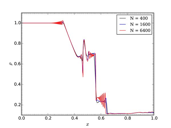
Figure 1: Total mass density for the Brio-Wu shock tube problem at $t=0.1$. Simulation results with three different resolutions are shown with black ($N=400$), blue ($N=1600$), and red ($N=6400$) lines, respectively.

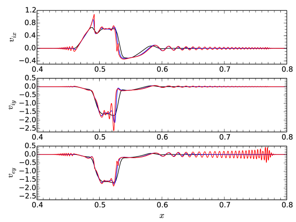
Figure 2: Closeup view of ion and electron velocities for the Brio-Wu shock tube problem at $t=0.02$. The $x$ (top) and $y$ (middle) components of ion velocity and $y$ component of electron velocity (bottom) are shown. The meaning of the color is the same as the previous figure.

The first test problem is an extension of 1D Riemann problem proposed by Brio & Wu (1988) that is one of the standard test problems for the ideal MHD. It has also been tested by the EMTF model, which clearly demonstrates the appearance of dispersive features (e.g., Hakim et al., 2006; Kumar & Mishra, 2012).

At the initial condition, the simulation box of unit length $0\leq x\leq 1$ was divided into the left and right states at the center $x=0.5$. Their physical quantities were specified respectively as follows

$$\begin{pmatrix}\rho\\ p\\ B_{x}/\sqrt{4\pi}\\ B_{y}/\sqrt{4\pi}\end{pmatrix}_{\rm left}=\begin{pmatrix}1.0\\ 1.0\\ 0.75\\ 1.0\\ \end{pmatrix},\qquad\begin{pmatrix}\rho\\ p\\ B_{x}/\sqrt{4\pi}\\ B_{y}/\sqrt{4\pi}\end{pmatrix}_{\rm right}=\begin{pmatrix}0.1\\ 0.125\\ 0.75\\ -1.0\end{pmatrix},$$ (55)

where $\rho\equiv\rho_{i}+\rho_{e}$ and $p\equiv p_{i}+p_{e}$ are the total mass density and total pressure, respectively. Other quantities were zero everywhere at the initial condition. This setup is identical to the original Brio-Wu shock tube problem for the ideal MHD. However, the parameter $q_{i}/m_{i}$ can be chosen arbitrarily to control the ion inertial length $\lambda_{i}\propto(q_{i}/m_{i})^{-1}$. Clearly, the ideal MHD corresponds to the limit $q_{i}/m_{i}\rightarrow\infty\,(\lambda_{i}\rightarrow 0)$. Here we chose $q_{i}/m_{i}$ such that $\lambda_{i}=10^{-3}/\sqrt{\rho}$. In this case, the problem is close to MHD but two-fluid nature will appear when sufficiently small grid size is used to resolve $\lambda_{i}$. For this problem, $\gamma=2$ was used instead of $5/3$. The ion to electron mass ratio was chosen to be $m_{i}/m_{e}=100$.

Fig. 1 shows snapshots of the total mass density $\rho$ at $t=0.1$ obtained with three different resolutions $N=400,1600,6400$ (i.e., $\Delta x=2.5\times 10^{-3},6.25\times 10^{-4},1.5625\times 10^{-4}$). At the lowest resolution (black), the grid size was comparable to or larger than the ion inertial length and dispersive nature was not clearly visible. Consequently, the numerical solution was almost the same as the MHD. In contrast, a clear dispersive wave train structure appeared behind the slow shock at around $x\sim 0.65$ in the medium resolution run (blue). Similar structures were also found at the leading edge of fast mode rarefaction propagating to the left ($x\sim 0.3$), as well as around a compound wave ($x\sim 0.5$). These features became further pronounced in the solution with the highest resolution. It is interesting that such dispersive waves are clearly visible even with such a small ion inertial length. We found that the propagation speed of the slow shock appears to be slower than the MHD result. This seems to be consistent with the result presented by Hakim et al. (2006). This may be understood to be due to a finite Poynting flux carried by the dispersive waves behind the shock.

It is noted that at this time ($t=0.1$) whistler waves emitted to the right had already reached to the right-hand boundary, which is, however, barely visible in the mass density profile. The propagation of whistler waves can more clearly be identified in the velocity profiles at earlier times. Closeup view of the ion and electron velocities at $t=0.02$ shown in Fig. 2 displays the propagation of whistler waves in both positive and negative directions again for three different resolutions. Note that the normal component of ion and electron velocities are identical in 1D because $\left(\nabla\times\mathbf{B}\right)_{x}=0$.

We see that as increasing the spatial resolution, the leading edge of whistler waves became more and more extended. In particular for the whistlers propagating to the right, the wavelength of the transverse electron velocity oscillations decreased in the positive $x$ direction. This is clearly due to dispersive nature of whistler waves. Namely, since the whistler waves have dispersion relation $\omega\propto k^{2}$ for $|\Omega_{ci}|\ll\omega\ll|\Omega_{ce}|$, the group velocity becomes higher for shorter wavelength modes. Note that the maximum wave propagation velocity (both group and phase velocity) was limited by finite electron inertia effect in the highest resolution run because the grid size was comparable to the electron inertial length for this simulation ($m_{i}/m_{e}=100$). If the spatial resolution is insufficient to resolve these small-scale features, numerical dissipation automatically damps out these waves.

Here, we have actually confirmed that our numerical simulation code automatically reduces essentially to ideal MHD when the grid size is larger than the ion inertial length. Since high frequency waves such as electromagnetic and Langmuir waves are absent, numerical stability only requires the CFL condition with respect to MHD characteristic speeds. We think this is a crucial advantage over the EMTF model.

4.2 Circularly Polarized Wave

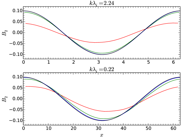
Figure 3: Profiles of the in-plane wave magnetic field component obtained by the circularly polarized wave problem. The highest frequency case $k\lambda_{i}\approx 2.24$ (top), and lowest frequency case $k\lambda_{i}\approx 0.22$ (bottom) are shown respectively. Results for four different resolutions are shown with red ($N=16$), green ($N=32$), blue ($N=64$), and black ($N=128$) lines, respectively. Note that the blue and black lines almost coincide in this figure. Likewise, the exact solutions are indistinguishable from the highest resolution results.

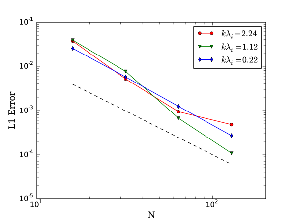
Figure 4: Convergence of L1 error for the in-plane wave magnetic field component as a function of the number of grid $N$ for the circularly polarized wave problem. Convergence for three different wavenumber cases is shown with different colors: red for $k\lambda_{i}\approx 2.24$, green for $k\lambda_{i}=1.12$, and blue for $k\lambda_{i}\approx 0.22$. The black dashed line indicates the theoretical second order convergence for reference.

It has been well known that a finite amplitude circularly polarized Alfvén wave propagating along the ambient magnetic field ($\mathbf{B}_{0}$) is an exact solution to the ideal MHD equations (e.g., Goldstein, 1978). Therefore, it is commonly used as a benchmark problem to test the accuracy of a numerical scheme.

Generalization of the MHD exact solution to the QNTF model is possible. Actually, the dispersion relation of a finite amplitude circularly polarized electromagnetic wave is identical to the corresponding linear dispersion relation

$$1+\left(\frac{\omega_{pi}}{kc}\right)^{2}\frac{\omega}{\omega+\Omega_{ci}}+\left(\frac{\omega_{pe}}{kc}\right)^{2}\frac{\omega}{\omega+\Omega_{ce}}=0,$$ (56)

where $\Omega_{cs}=q_{s}B_{0}/m_{s}c$ is the cyclotron frequency. The positive (negative) $\omega$ in the above dispersion relation indicates right-handed (left-handed) polarization. Adopting a coordinate system with orthogonal unit vectors $\mathbf{e}_{i}\,(i=1,2,3)$ such that $\mathbf{e}_{1}$ is parallel to the background field, $\mathbf{e}_{2}$ is a vector perpendicular to $\mathbf{e}_{1}$, and $\mathbf{e}_{3}=\mathbf{e}_{1}\times\mathbf{e}_{2}$, we can write the eigenvector corresponding to the solution of the dispersion relation as follows

$$B_{2}=\xi B_{0}\cos(kx-\omega t),\quad B_{3}=\xi B_{0}\sin(kx-\omega t),$$ (57)

$$v_{s,2}=V_{s}\cos(kx-\omega t),\quad v_{s,3}=V_{s}\sin(kx-\omega t),$$ (58)

where

$$V_{s}=-\xi\frac{\Omega_{cs}}{\omega+\Omega_{cs}}\frac{\omega}{k}.$$ (59)

The amplitude of the wave $\xi$ normalized to the background magnetic field $B_{0}$ is a free parameter that can be chosen arbitrarily. Nevertheless, since the finite amplitude wave may suffer a parametric instability (e.g., Goldstein, 1978; Terasawa et al., 1986), we chose a small value $\xi=0.1$ to suppress possible growth of the instability during the simulation.

We set up a 2D simulation box with the computational domain $0\leq x\leq 2L$, $0\leq y\leq L$ with the periodic boundary condition in both directions. The simulation box was resolved by $2N\times N$ grid points (i.e., $\Delta x=\Delta y$). The background magnetic field was inclined with respect to the $x$ axis by an angle $\theta=\tan^{-1}(2)$. The wavenumber of a finite amplitude circularly polarized wave was chosen as $(k_{x},k_{y})=(\pi/L,2\pi/L)$ (i.e., mode = 1 in each direction). The initial condition was set up by rotating the exact solution by an angle $\theta$ such that $\mathbf{e}_{1}$ is parallel to the background magnetic field and $\mathbf{e}_{2}$ is in the simulation plane. Since the wave propagates oblique to the grid, this provides a benchmark problem to test the accuracy of handling smooth profiles in multidimensions. In this simulation, time and length were normalized to the ion cyclotron frequency $\Omega_{ci}$ and ion inertial length $\lambda_{i}=c/\omega_{pi}$, respectively. The ambient magnetic field strength was chosen to be $B_{0}=\sqrt{4\pi}$.

By appropriately choosing $L/\lambda_{i}$, one may test the code performance for different parameter regimes. We here discuss three different physical wavenumber cases, $k\lambda_{i}\approx 2.24,1.12,0.22$ (corresponding to $L/\lambda_{i}=\pi,2\pi,10\pi$, respectively). The wave frequencies were respectively determined as $\omega/\Omega_{ci}\approx 5.72,1.89,0.25$ by solving the dispersion relation for right-handed polarization ($\omega>0$). The lowest frequency case is essentially an Alfvén wave in the MHD regime, whereas higher frequency cases correspond to dispersive whistler waves. In all cases, a plasma beta of $\beta=0.1$, and an ion to electron mass ratio of $m_{i}/m_{e}=256$ were used.

Fig. 3 shows the profiles of the in-plane component of wave magnetic field $B_{2}=(-2B_{x}+B_{y})/\sqrt{5}$ as functions of $x$ (i.e., cut through $y=0$) after five wave periods. Results with the highest and lowest frequency runs are shown in top and bottom panels, respectively. The amplitude is normalized to the background field $B_{0}$. The simulations were performed with four different resolutions $N=16,32,64,128$ for each case. We see that in both cases the numerical solutions converged to the analytic ones as increasing the resolution. Note that the initial conditions (or exact solutions) are indistinguishable from the highest resolution results and are not shown.

The error convergence is shown in Fig. 4 for three different wavenumbers. The L1 errors shown in this plot are those of the $B_{2}$ component evaluated as

$$L1(B_{2})=\frac{1}{2N^{2}B_{0}}\sum_{i,j}\left|B_{2;i,j}(t=5T)-B_{2;i,j}(t=0)\right|,$$ (60)

where $T$ denotes a wave period. This confirms that the code achieved roughly second order convergence (which is shown by the dashed line for reference). However, the error behavior became irregular for the higher frequency cases at high resolution. We have performed simulations with other wavenumbers and/or mass ratios, and confirmed that this irregular convergence appears when the grid size becomes comparable to or smaller than the electron inertial length. This may thus partly be related to the simplified estimate of the maximum characteristic speeds that is not strictly correct at this scale. In any case, since our primary focus is not on this small scale, we have not attempted to resolve the issue.

4.3 Orszag-Tang Vortex

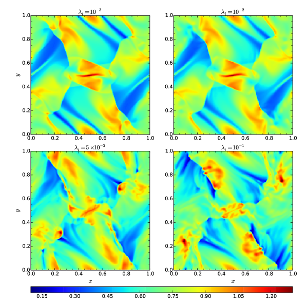
Figure 5: Temperature distribution for the Orszag-Tang vortex problem at $t=0.5$. The solutions with different initial ion inertial lengths are shown; $\lambda_{i}=10^{-3}$ (top left), $10^{-2}$ (top right), $5\times 10^{-2}$ (bottom left), $10^{-1}$ bottom right.

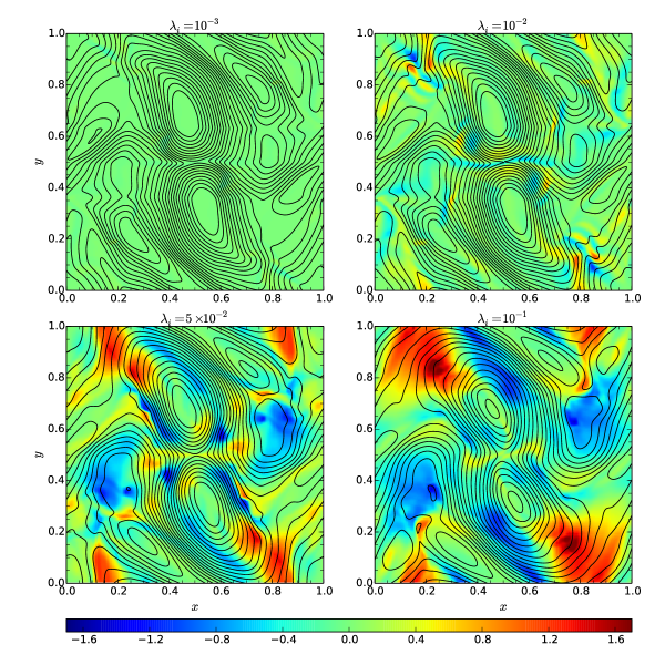
Figure 6: Out-of-plane magnetic field component $B_{z}$ and the vector potential $A_{z}$ for the Orszag-Tang vortex problem at $t=0.5$. The color indicates $B_{z}$, while black lines are contours of $A_{z}$ (magnetic field lines in the $x{\rm-}y$ plane), respectively. The format is the same as the previous figure.

The Orszag-Tang vortex problem has been one of the most standard benchmark problems for multidimensional MHD codes. It starts with a smooth initial profile, but the solution soon becomes complex involving many discontinuities. Therefore, it has been used to test the capability of handling multidimensional discontinuities which may introduce non-negligible magnetic monopoles in the numerical solution. On the other hand, to the authors knowledge, numerical results obtained with the Hall-MHD and/or EMTF models have not been published in the literature. Although there were numerical studies with similar but different initial conditions (e.g., Matthews et al., 1995; Perri et al., 2012), they are not useful for comparison with the present results. Therefore, we generalize the original problem to the parameter regime where the Hall term starts to play a role, but without changing the initial condition so that comparison with published results becomes easier.

The computational domain was a unit square $0\leq x\leq 1$, $0\leq y\leq 1$ with the periodic boundary condition in both directions. The initial condition was given by the smooth profile

$$v_{x}=-\sin\left(2\pi y\right),\quad v_{y}=\sin\left(2\pi x\right),$$ (61)

$$B_{x}=-B_{0}\sin\left(2\pi y\right),\quad B_{y}=B_{0}\sin\left(4\pi x\right),$$ (62)

where $B_{0}=\sqrt{4\pi}$. The density and pressure were constant; $\rho=\gamma^{2},p=\gamma$, and out-of-plane velocity and magnetic field components were zero $v_{z}=B_{z}=0$. This definition is identical to the standard MHD test problem (except for normalization). Again, one needs to specify the ion inertial length (or $q_{i}/m_{i}$) relative to the box size.

Numerical results with four different initial ion inertial lengths $\lambda_{i}=10^{-3},10^{-2},5\times 10^{-2},10^{-1}$ are shown in Figs. 5 and 6. We used $200\times 200$ grid points and $m_{i}/m_{e}=100$ in all the simulation runs. Fig. 5 displays snapshots of the temperature distribution at $t=0.5$. (Here, the temperature is defined with the total pressure and mass density as $p/\rho$.) In Fig. 6, the color indicates the out-of-plane component of the magnetic field normalized to $B_{0}$, whereas the black solid lines are contours of the vector potential $A_{z}$ (i.e., magnetic field lines in the plane) at the same instant of time. We confirmed that the $\nabla\cdot\mathbf{B}$ error in the numerical solutions was on the order of round-off error, which is consistent with the design of the numerical scheme.

Since the grid size was $\Delta x=5\times 10^{-3}$, the run with the smallest ion inertial length $\lambda_{i}=10^{-3}$ did not resolve the ion scale. It was thus essentially in the MHD regime and the results may be compared with published results for ideal MHD. We see that our simulation well captured discontinuities and other small scale features. This is not surprising because in this case our scheme becomes almost the same as the second order scheme described in Londrillo & Del Zanna (2004) except for subtleties. Although the overall structures were similar in all the cases, dispersive features clearly appeared in the numerical solutions as increasing the ion inertial length. The fact that the Hall term played the role in the numerical solutions can most clearly be visible in Fig. 6 because the out-of-plane magnetic field disappears in the ideal MHD limit. Even in the case with $\lambda_{i}=10^{-2}$, in which the temperature distribution looks almost unchanged from the MHD result, amplitude of $B_{z}$ became substantial (at around $x\sim 1.5,y\sim 0.9$ and its symmetric point). For larger ion inertial lengths, the solution became much more complex even in this early stage of evolution.

The numerical results clearly indicate that it is possible to implement the two-fluid effect in a shock-capturing code without loosing its advantages. A shock-capturing code gives a non-oscillatory solution when encountered by discontinuities by automatically introducing required dissipation. On the other hand, dispersive character must be retained at ion and electron inertial scales, which tends to produce an oscillatory solution. Our numerical simulation code successfully implements these two contradictory features at the same time without suffering from numerical instability.

4.4 Magnetic Reconnection

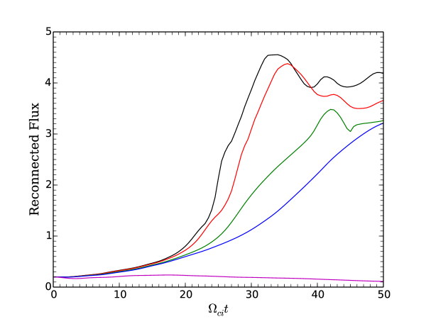
Figure 7: Time evolution of reconnected magnetic flux for the magnetic reconnection problem. Five runs with different normalized resistivities are shown in different colors. The black, red, green, blue, magenta lines correspond to $\eta^{\star}=0,10^{-6},5\times 10^{-6},10^{-5},10^{-4}$, respectively.

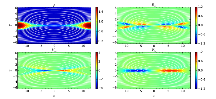
Figure 8: Snapshots for the magnetic reconnection problem at $\Omega_{ci}t=21.5$ for the run with $\eta^{\star}=0$. Shown are the mass density (top left), out-of-plane magnetic field component (top right), $x$ component of electron velocity (bottom left), and ion velocity (bottom right). The white lines in each panel shows the magnetic field lines (contour lines for the vector potential $A_{z}$). At this time, the reconnected magnetic flux reached $\psi(t)=1.0$.

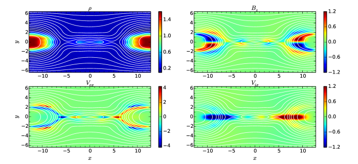
Figure 9: Snapshots for the magnetic reconnection problem at $\Omega_{ci}t=25.0$ (corresponds to the time $\psi(t)=2.0$) for the run with $\eta^{\star}=0$. The format is the same as the previous figure.

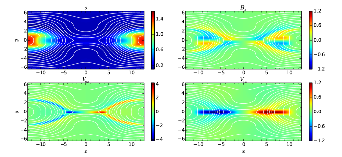
Figure 10: Snapshots for the magnetic reconnection problem at $\Omega_{ci}t=31.5$ (corresponds to the time $\psi(t)=2.0$) for the run with $\eta^{\star}=5\times 10^{-6}$. The format is the same as the previous figure.

Our final test problem is the GEM magnetic reconnection challenge problem that has been well tested with many different simulation models (Birn et al., 2001). Here we use this problem to test the effect of resistivity. The initial condition was given by the Harris equilibrium which is identical to the one described in Birn et al. (2001). The magnetic field and number density profiles were given by

$$B_{x}(y)=B_{0}\tanh\left(y/d\right)$$ (63)

and

$$n(y)=n_{0}\operatorname{sech}^{2}\left(y/d\right)+n_{bg},$$ (64)

respectively. Here, the width of the current sheet is represented by $d$. The ion and electron temperatures were determined by the pressure balance condition $n_{0}(T_{i}+T_{e})=B_{0}^{2}/8\pi$. We here used a temperature ratio of $\tau=5$ to be consistent with the original problem. The ion and electron drift velocities in the $z$ direction must satisfy the relation $\tau=-v_{i,z}/v_{e,z}$ for the initial condition to be a Vlasov-Maxwell equilibrium. The drift velocities were thus initialized as

$$v_{i,z}=-\frac{cB_{0}}{4\pi e}\frac{\tau}{1+\tau}\frac{n_{0}\operatorname{sech}^{2}(y/d)}{n_{0}\operatorname{sech}^{2}\left(y/d\right)+n_{bg}},$$ (65)

$$v_{e,z}=+\frac{cB_{0}}{4\pi e}\frac{1}{1+\tau}\frac{n_{0}\operatorname{sech}^{2}(y/d)}{n_{0}\operatorname{sech}^{2}\left(y/d\right)+n_{bg}}$$ (66)

for ions and electrons, respectively. Other quantities were initialized with zero.

The normalization of time and space was such that the ion cyclotron frequency $\Omega_{ci}=eB_{0}/m_{i}c=1$ and the ion inertial length $c/\omega_{pi}=c\sqrt{m_{i}/4\pi n_{0}e^{2}}=1$. Accordingly, the velocity was normalized to the ion Alfvén speed $V_{A,i}=B_{0}/\sqrt{4\pi n_{0}m_{i}}$. Note that in the normalized unit, $B_{0}/\sqrt{4\pi}=n_{0}=m_{i}=1$. We used a rectangular simulation domain $-L\leq x\leq+L$ and $-L/2\leq y\leq+L/2$ with $L=12.8$. The current sheet thickness was taken to be $d=0.5$. The simulations were performed with $256\times 128$ grid points with a mass ratio of $m_{i}/m_{e}=25$. The grid size $\Delta x=\Delta y=0.1$ was thus roughly comparable to the electron inertial length for the initial current sheet density. The periodic boundary condition was used in $x$ direction, while the conducting wall boundary was used in $y$ direction.

To initiate magnetic reconnection, the initial magnetic field was perturbed with the out-of-plane component of the vector potential given by

$$\Phi=\Phi_{0}\frac{\pi B_{0}}{L}\cos\left(\frac{\pi x}{L}\right)\cos\left(\frac{\pi y}{L}\right)$$ (67)

where $\Phi_{0}=0.1$. With this initial condition, the X-point was located initially at the origin from which the reconnection process started to evolve.

Fig. 7 shows time evolution of reconnected magnetic flux for simulations with five different normalized resistivities: $\eta^{\star}=0,10^{-6},5\times 10^{-6},10^{-5},10^{-4}$. Recall that since the resistivity is normalized with respect to the local plasma frequency, the diffusivity depends on the local density even with a spatially constant resistivity. The reconnected flux was computed by

$$\psi(t)=\frac{1}{2B_{0}}\int_{-L}^{+L}|B_{y}(x,y=0,t)|dx.$$ (68)

In all cases except for $\eta^{\star}=10^{-4}$, the reconnection rates estimated from the slope of reconnected flux exceeded $\sim 0.1$ in the nonlinear phase, consistent with published results.

Fig. 8 shows snapshots at $\Omega_{ci}t=21.5$ for $\eta^{\star}=0$, at which the normalized reconnected flux reached $\psi(t)=1.0$. Fast outflows originating from the X-point are clearly seen for both ion and electron velocities. The ions and electrons were accelerated to the Alfvén speeds defined for each species ($V_{A,i}$ for ions and $V_{A,e}=\sqrt{m_{i}/m_{e}}V_{A,i}$ for electrons). The out-of-plane magnetic field $B_{z}$ was generated in association with the decoupling between ion and electron dynamics. Similar characteristics were also found in other runs at the time such that $\psi(t)=1.0$, although the magnitude decreased with increasing the resistivity. These features are consistent with previous numerical studies.

There was a quantitative difference in the time evolution of reconnected flux in between $\eta^{\star}=10^{-6}$ and $5\times 10^{-6}$ after $\Omega_{ci}t\gtrsim 25$. We found that the further increase in the reconnection rate in smaller resistivity runs was associated with the formation of secondary magnetic islands. Figs. 9 and 10 compare runs with $\eta^{\star}=0$ and $5\times 10^{-6}$ at the time when the same amount of flux was reconnected $\psi(t)=2.0$ ($\Omega_{ci}t=25.0$ and $31.5$ respectively). Two newly formed X-points in the elongated thin current sheet can be seen in Fig. 9, whereas the dynamics was still dominated by a single X-point in Fig. 10. Formation of secondary magnetic islands was not observed until the end of simulations $\Omega_{ci}t=50$ for $\eta^{\star}\geq 5\times 10^{-6}$. This difference may be understood from the viewpoint of the stability of the thin (i.e., electron-scale) current sheet generated in the nonlinear phase of reconnection process. In higher resistivity runs, the length of the thin current sheet characterized by the fast electron outflow became shorter because of the diffusion during the propagation. This is probably the reason for prohibiting the excitation of a secondary tearing mode. The electron-scale current sheet may also become unstable against another instability in fully 3D simulations (Drake et al., 1994). Nevertheless, one must bare in mind that electron kinetic physics, which is not included in the present model, will play a role in the dynamics of such a thin current sheet.

5 Conclusions

In the present paper, we have proposed the QNTF model for collisionless plasmas. The basic equations are the fluid equations for ions and electrons and the Maxwell equations without displacement current. The absence of the displacement current indicates the charge neutrality, which is a reasonable assumption for low frequency phenomena. Rewriting the basic equations, it is shown that the system consists of the conservation laws for five scalar variables (total mass, momentum, and energy), and the induction equation for the magnetic field, supplemented by the generalized Ohm’s law. The system fully takes into account finite electron inertia effect, which introduces the upper bound to the phase speed of whistler waves. On the other hand, it reduces to the ideal MHD in the long wavelength limit. No high frequency waves (such as Langmuir or electromagnetic waves) exist in the system, which would otherwise impose a severe restriction on the simulation time step even in the long wavelength limit.

We have developed a 3D numerical simulation code for solving the QNTF equations. The code employs the HLL approximate Riemann solver combined with the UCT method for the induction equation. With this approach, we avoid complicated characteristic decomposition with keeping the advantage of a shock-capturing scheme. The UCT scheme guarantees the divergence-free condition for the magnetic field up to machine accuracy, without loosing upwind property. Therefore, the code is able to capture complicated multidimensional sharp discontinuities without appreciable numerical oscillation. At the same time, it successfully describes dispersive waves arising from the two-fluid effect without numerical problem. The upper bound of whistler wave phase speed appropriately introduced by finite electron inertia helps to overcome the well-known numerical stability issue in dealing with the short wavelength mode.

In the numerical examples, we have confirmed that the numerical solutions reduce to the ideal MHD results when the ion inertial length is small enough. In this case, numerical stability requires only the CFL condition with respect to the MHD characteristic speed because of the absence of high frequency waves. This is in clear contrast to the EMTF equations in which high frequency waves must be resolved by the simulation time step. Since these waves will not play a major role in non-relativistic plasmas, the low frequency approximation is adequate. Consequently, we believe that the QNTF model offers a better alternative to the Hall-MHD and/or EMTF models.

Appendix A Derivation of Generalized Ohm’s Law

We here introduce a collision term in the right-hand side of the equation of motion for the two fluids to take into account finite resistivity $\eta$. It is intended to be rather phenomenological (or anomalous) such as due to kinetic wave-particle interactions. The collision term is defined as

$$\mathbf{R}_{i}=-\mathbf{R}_{e}=-\frac{\eta}{4\pi}\frac{\omega_{pe}^{2}+\omega_{pi}^{2}}{\dfrac{q_{i}}{m_{i}}-\dfrac{q_{e}}{m_{e}}}\left(\frac{q_{i}}{m_{i}}\rho_{i}\mathbf{v}_{i}+\frac{q_{e}}{m_{e}}\rho_{e}\mathbf{v}_{e}\right)=-\frac{\eta}{4\pi}\frac{\omega_{p}^{2}}{\dfrac{q_{i}}{m_{i}}-\dfrac{q_{e}}{m_{e}}}\mathbf{J}$$ (69)

where $\mathbf{R}_{i}$ and $\mathbf{R}_{e}$ are for ion and electron fluids respectively. By adding it into the equation of motion, one may take into account effective friction between the species. It is easy to understand from the symmetry that the definition does not violate the momentum conservation law.

The generalized Ohm’s law Eq. (12) used in this paper may be obtained by taking a weighted sum between the two equations with the weight factor $q_{s}/m_{s}$. This yields

$$\frac{\partial}{\partial t}{\mathbf{J}}+\nabla\cdot\left[\sum_{s}\frac{q_{s}}{m_{s}}\left(\rho_{s}{\mathbf{v}}_{s}{\mathbf{v}}_{s}+p_{s}{\mathbf{I}}\right)\right]=\sum_{s}\left[\rho_{s}\frac{q_{s}^{2}}{m_{s}^{2}}{\mathbf{E}}+\rho_{s}\frac{q_{s}^{2}}{m_{s}^{2}}\frac{{\mathbf{v}}_{s}}{c}\times{\mathbf{B}}\right]-\frac{\eta}{4\pi}\omega_{p}^{2}\mathbf{J}.$$ (70)

Using Faraday’s law, the first term may be rewritten as follows

$$\frac{\partial}{\partial t}{\mathbf{J}} =\frac{c}{4\pi}\nabla\times\frac{\partial}{\partial t}{\mathbf{B}}$$

$$=-\frac{c^{2}}{4\pi}\nabla\times\nabla\times{\mathbf{E}}.$$ (71)

Now rearranging the equation, we arrive at

$$\left(\sum_{s}\omega_{ps}^{2}\right){\mathbf{E}}+c^{2}\nabla\times\nabla\times{\mathbf{E}}=-\left(\sum_{s}\omega_{ps}^{2}\frac{{\mathbf{v}}_{s}}{c}\right)\times{\mathbf{B}}+\nabla\cdot\left(\sum_{s}\frac{4\pi q_{s}}{m_{s}}\left(\rho_{s}{\mathbf{v}}_{s}{\mathbf{v}}_{s}+p_{s}{\mathbf{I}}\right)\right)+\eta\omega_{p}^{2}\mathbf{J},$$ (72)

which is identical to Eq. (12). It should be noted that contributions from both ion and electron fluids are fully taken into account in this form of Ohm’s law, so that it always provides the correct equation regardless of the ion-to-electron mass ratio.

Appendix B Linear Dispersion Analysis

Here we outline the linear dispersion analysis for the QNTF model. We consider a homogeneous electron-proton plasma without resistivity, i.e., $q_{i}=-q_{e}=e$ and $\eta=0$. The ion fluid equations, the generalized Ohm’s law, and the induction equation are used. Hereafter, we drop the subscript for the particle species unless necessary, and the fluid quantities without subscript must be read as the ion quantities. In addition, we use the definition for the thermal velocity $V_{i}^{2}=\gamma k_{B}T_{i}/m_{i},V_{e}^{2}=\gamma k_{B}T_{e}/m_{e}$ (where $k_{B}$ is the Boltzmann constant) and the following notation: $\varepsilon=m_{e}/m_{i}$, $\tau=T_{i}/T_{e}$, $\mu=\varepsilon(1-\tau\varepsilon)/(1+\varepsilon)$. Note that in the derivation below, the assumption of constant $\tau$ is not necessary.

It is easy to obtain the following equation from the linearized ion fluid equations

$$\left(\omega^{2}-V_{i}^{2}\mathbf{k}\mathbf{k}\right)\cdot\delta\mathbf{v}=i\omega\frac{e}{m_{i}}\left(\delta\mathbf{E}+\frac{\delta\mathbf{v}}{c}\times\mathbf{B}_{0}\right),$$ (73)

whereas for the generalized Ohm’s law, we have

$$\left(\omega_{p}^{2}-c^{2}\mathbf{k}\times\mathbf{k}\times\right)\delta\mathbf{E}=-\frac{\delta\mathbf{\Gamma}}{c}\times\mathbf{B}_{0}+i\mathbf{k}\cdot\delta\mathbf{\Pi},$$ (74)

with

$$\delta\mathbf{\Gamma}=\omega_{p}^{2}\left\{\delta\mathbf{v}-\frac{m_{i}}{e}\frac{c}{4\pi\rho_{0}(1+\varepsilon)}i\mathbf{k}\times\delta\mathbf{B}\right\}$$ (75)

$$\delta\mathbf{\Pi}=-\omega_{p}^{2}\frac{m_{i}}{e}\mu V_{e}^{2}\frac{\mathbf{k}\cdot\delta\mathbf{v}}{\omega}.$$ (76)

Rearranging the above equation using $\delta\mathbf{B}=c\mathbf{k}/\omega\times\delta\mathbf{E}$, we obtain

$$i\omega\frac{e}{m_{i}}\left(\delta\mathbf{E}+\frac{\delta\mathbf{v}}{c}\times\mathbf{B}_{0}\right)=\mu V_{e}^{2}\mathbf{k}\mathbf{k}\cdot\delta\mathbf{v}+i\frac{e}{m_{i}}\lambda^{2}\left[\varepsilon\omega\mathbf{k}\times\mathbf{k}\times\delta\mathbf{E}-i\mathbf{\Omega}_{ci}\times\mathbf{k}\times\mathbf{k}\times\delta\mathbf{E}\right],$$ (77)

where we have defined $\lambda^{2}=V_{A}^{2}/\Omega_{ci}^{2}=c^{2}/\omega_{pi}^{2}(1+\varepsilon)$ and $\mathbf{\Omega}_{ci}=\Omega_{ci}\mathbf{B}_{0}/B_{0}$, respectively.

Now our task is to eliminate $\delta\mathbf{v}$ from Eqs. (73) and (77), to get a dispersion matrix $\mathbf{D}$ satisfying

$$\mathbf{D}\cdot\delta\mathbf{E}=\mathbf{0},$$ (78)

from which the dispersion relation is naturally obtained as $|\mathbf{D}|=0$. For this purpose, we introduce the following matrix notation:

$$\mathbf{M} \equiv\omega^{2}\mathbf{I}-V_{S}^{2}\mathbf{k}\mathbf{k}$$ (79)

$$k^{2}\mathbf{N}\cdot\delta\mathbf{E} \equiv i\mathbf{\Omega}_{ci}\times\mathbf{k}\times\mathbf{k}\times\delta\mathbf{E}-\varepsilon\omega\mathbf{k}\times\mathbf{k}\times\delta\mathbf{E}$$ (80)

$$\mathbf{W}\cdot\delta\mathbf{v} \equiv\mathbf{\Omega}_{ci}\times\delta\mathbf{v},$$ (81)

where the sound speed is defined by

$$V_{S}^{2}\equiv V_{i}^{2}+\mu V_{e}^{2}=\frac{\gamma k_{B}(T_{i}+T_{e})}{m_{i}+m_{e}}.$$ (82)

Solving the equations with respect to the ion velocity, we have

$$\delta\mathbf{v}=-i\frac{e}{m_{i}}k^{2}\lambda^{2}\mathbf{M}^{-1}\cdot\mathbf{N}\cdot\delta\mathbf{E}.$$ (83)

Substituting this into the generalized Ohm’s law Eq. (77), we finally obtain

$$\mathbf{D}=\mathbf{I}+k^{2}\lambda^{2}\left[i\mathbf{W}\cdot\mathbf{M}^{-1}\cdot\mathbf{N}+\mu\frac{V_{e}^{2}}{\omega}\mathbf{k}\mathbf{k}\cdot\mathbf{M}^{-1}\cdot\mathbf{N}+\frac{1}{\omega}\mathbf{N}\right]$$ (84)

as the dispersion matrix.

Explicit form of the normalized dispersion matrix is given as follows:

$$\mathbf{D}=\frac{1}{X^{2}(X^{2}-\beta)}\left[\mathbf{D}_{MHD}+\mathbf{D}_{i}+\mathbf{D}_{e}\right],$$ (85)

where

$$\mathbf{D}_{MHD} =\begin{pmatrix}(X^{2}-\beta^{2})(X^{2}-\cos^{2}\theta)&0&(X^{2}-\beta^{2})\cos\theta\sin\theta\\ 0&X^{4}-(\beta^{2}+1)X^{2}+\beta^{2}\cos^{2}\theta&0&\\ 0&0&X^{2}(X^{2}-\beta^{2})&\end{pmatrix},$$ (86)

$$\mathbf{D}_{i} =i\kappa X\begin{pmatrix}0&X^{2}-\beta^{2}+\mu\beta_{e}^{2}\sin^{2}\theta&0&\\ -(X^{2}-\beta^{2})\cos^{2}\theta&0&(X^{2}-\beta^{2})\cos\theta\sin\theta\\ 0&\mu\beta_{e}^{2}\cos\theta\sin\theta&0&\end{pmatrix},$$ (87)

$$\mathbf{D}_{e} =i\varepsilon\kappa X(X^{2}-\beta^{2})\begin{pmatrix}-i\kappa X\cos^{2}\theta&-1&i\kappa X\cos\theta\sin\theta&\\ \cos^{2}\theta&-i\kappa X&-\cos\theta\sin\theta&\\ i\kappa X\cos\theta\sin\theta&0&-i\kappa X\sin^{2}\theta&\end{pmatrix}.$$ (88)

In the above expression, $X=\omega/kV_{A}$ is the normalized phase speed, $\kappa=k\lambda$ is the normalized wavenumber, $\theta$ is the wave propagation angle with respect to the ambient magnetic field. We also defined $\beta=V_{S}^{2}/V_{A}^{2}$ and $\beta_{e}=V_{e}^{2}/V_{A}^{2}$, respectively.

One may easily understand that $\mathbf{D}_{MHD}$ (which remains finite for $\kappa\rightarrow 0$) corresponds to the MHD limit. On the other hand, $\mathbf{D}_{i}$ (independent of $\varepsilon$) and $\mathbf{D}_{e}$ represent respectively the ion and electron inertia effects. Taking the determinant, and arranging it into the polynomial form, we obtain the dispersion relation given in Eq. (49). Most of cumbersome calculation presented in the derivation has been performed with a computer algebra system package SymPy (SymPy Development Team, 2014).

Since the highest phase speed appears at the parallel propagation, we here investigate this special case in detail. For the parallel propagation, the sound mode decouples from the electromagnetic modes, and the dispersion relation may be factorized as follows

$$(X^{2}-\beta)\left\{(1+\varepsilon\kappa^{2})^{2}X^{4}-(2+(1+\varepsilon^{2})\kappa^{2})X^{2}+1\right\}=0.$$ (89)

The dispersion relation for electromagnetic waves corresponding to the second factor (i.e., the curly bracket) is shown in Fig. 11. It is clearly seen that the wave frequency approaches to the electron cyclotron frequency at the short wavelength limit. The phase speed, on the other hand, has a maximum at around $\kappa\simeq\sqrt{m_{i}/m_{e}}$ (i.e., $kc/\omega_{pe}\simeq 1$) and the maximum phase speed is given approximately by $X\simeq\sqrt{m_{i}/m_{e}}/2$.

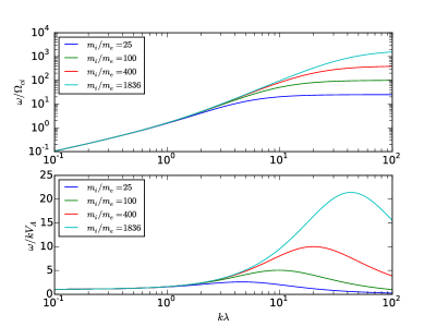
Figure 11: Linear dispersion relation for electromagnetic waves propagating parallel to the ambient magnetic field. Wave frequencies as functions of wavenumber are shown in the top panel for four different mass ratios $m_{i}/m_{e}=25,100,400,1836$. Corresponding phase speeds are shown in the bottom panel. Only the waves with maximum phase speed (i.e., on the whistler branch) are shown.

Note that, in a previous publication, we have shown that the deviation from the Hall-MHD dispersion $\omega\propto k^{2}$ occurs approximately at $\kappa\simeq(m_{i}/m_{e})^{1/4}$ (Amano et al., 2014, Appendix, B.). The weak dependence of the critical wavenumber on the mass ratio indicates that, at scale length on the order of or larger than the ion inertial length, the result should not depend strongly on the reduced mass ratio.

References

- Amano et al. (2014) Amano, T., Higashimori, K., & Shirakawa, K. (2014). A robust method for handling low density regions in hybrid simulations for collisionless plasmas. Journal of Computational Physics, 275, 197–212.
- Amano & Kirk (2013) Amano, T., & Kirk, J. G. (2013). The Role of Superluminal Electromagnetic Waves in Pulsar Wind Termination Shocks. The Astrophysical Jounral, 770, 18.
- Arnold et al. (2008) Arnold, L., Dreher, J., & Grauer, R. (2008). A semi-implicit Hall-MHD solver using whistler wave preconditioning. Computer Physics Communications, 178, 553–557.
- Balsara (1998) Balsara, D. S. (1998). Linearized Formulation of the Riemann Problem for Adiabatic and Isothermal Magnetohydrodynamics. The Astrophysical Jounral Supplement, 116, 119–131.
- Balsara (2001) Balsara, D. S. (2001). Divergence-Free Adaptive Mesh Refinement for Magnetohydrodynamics. Journal of Computational Physics, 174, 614–648.
- Balsara (2004) Balsara, D. S. (2004). Second-Order-accurate Schemes for Magnetohydrodynamics with Divergence-free Reconstruction. The Astrophysical Jounral Supplement, 151, 149–184.
- Balsara (2010) Balsara, D. S. (2010). Multidimensional HLLE Riemann solver: Application to Euler and magnetohydrodynamic flows. Journal of Computational Physics, 229, 1970–1993.
- Balsara (2012) Balsara, D. S. (2012). A two-dimensional HLLC Riemann solver for conservation laws: Application to Euler and magnetohydrodynamic flows. Journal of Computational Physics, 231, 7476–7503.
- Balsara & Spicer (1999) Balsara, D. S., & Spicer, D. S. (1999). A Staggered Mesh Algorithm Using High Order Godunov Fluxes to Ensure Solenoidal Magnetic Fields in Magnetohydrodynamic Simulations. Journal of Computational Physics, 149, 270–292.
- Birn et al. (2001) Birn, J., Drake, J. F., Shay, M. A., Rogers, B. N., Denton, R. E., Hesse, M., Kuznetsova, M., Ma, Z. W., Bhattacharjee, A., Otto, A., & Pritchett, P. L. (2001). Geospace Environmental Modeling (GEM) magnetic reconnection challenge. Jounral of Geophysical Research, 106, 3715–3720.
- Brio & Wu (1988) Brio, M., & Wu, C. C. (1988). An upwind differencing scheme for the equations of ideal magnetohydrodynamics. Journal of Computational Physics, 75, 400–422.
- Dai & Woodward (1998) Dai, W., & Woodward, P. R. (1998). A Simple Finite Difference Scheme for Multidimensional Magnetohydrodynamical Equations. Journal of Computational Physics, 142, 331–369.
- Del Zanna et al. (2003) Del Zanna, L., Bucciantini, N., & Londrillo, P. (2003). An efficient shock-capturing central-type scheme for multidimensional relativistic flows. II. Magnetohydrodynamics. Astronomy & Astrophysics, 400, 397–413.
- Del Zanna et al. (2007) Del Zanna, L., Zanotti, O., Bucciantini, N., & Londrillo, P. (2007). ECHO: a Eulerian conservative high-order scheme for general relativistic magnetohydrodynamics and magnetodynamics. Astronomy & Astrophysics, 473, 11–30.
- Drake et al. (1994) Drake, J. F., Kleva, R. G., & Mandt, M. E. (1994). Structure of thin current layers: Implications for magnetic reconnection. Physical Review Letters, 73, 1251–1254.
- Evans & Hawley (1988) Evans, C. R., & Hawley, J. F. (1988). Simulation of magnetohydrodynamic flows - A constrained transport method. The Astrophysical Jounral, 332, 659–677.
- Gardiner & Stone (2005) Gardiner, T. A., & Stone, J. M. (2005). An unsplit Godunov method for ideal MHD via constrained transport. Journal of Computational Physics, 205, 509–539.
- Goldstein (1978) Goldstein, M. L. (1978). An instability of finite amplitude circularly polarized Alfven waves. The Astrophysical Jounral, 219, 700–704.
- Hakim et al. (2006) Hakim, A., Loverich, J., & Shumlak, U. (2006). A high resolution wave propagation scheme for ideal Two-Fluid plasma equations. Journal of Computational Physics, 219, 418–442.
- Kumar & Mishra (2012) Kumar, H., & Mishra, S. (2012). Entropy stable numerical schemes for two-fluid plasma equations. Journal of Scientific Computing, 52, 401–425.
- Kurganov et al. (2001) Kurganov, A., Noelle, S., & Petrova, G. (2001). Semidiscrete central-upwind schemes for hyperbolic conservation laws and hamilton–jacobi equations. SIAM J. Sci. Comput., 23, 707–740.
- Kurganov & Tadmor (2000) Kurganov, A., & Tadmor, E. (2000). New High-Resolution Central Schemes for Nonlinear Conservation Laws and Convection-Diffusion Equations. Journal of Computational Physics, 160, 241–282.
- Kuznetsova et al. (1998) Kuznetsova, M. M., Hesse, M., & Winske, D. (1998). Kinetic quasi-viscous and bulk flow inertia effects in collisionless magnetotail reconnection. Jounral of Geophysical Research, 103, 199–214.